Holographic superconductors in a model of non-relativistic gravity

Abstract

Abstract

We have studied holographic superconductors with spherical symmetry in the Ho$\check{\textbf{r}}$ava-Lifshitz gravity by using a semi analytical method, and also we have calculated the critical temperature and shown when the condensation will appear in a similar pattern as in the Einstein-Gauss- Bonnet gravity. We have computed the dependency of the conductivity as a function of frequency in this new non-relativistic model of quantum gravity.

I Introduction

As a phenomenological fact, superconductivity is usually modeled by a Landau-Ginzburg Lagrangian where a complex scalar field develops a condensation in a superconductive phase. To have a scalar condensation in the boundary theory, Horowitz and his collaborators Horowitz introduced a U(1) gauge field and a conformally coupled charged complex scalar field in the black hole background.That potential corresponding to the conformal mass is negative,although above the Breitenlohner-Freedman (BF) bound Freedman it does not cause any instability in the theory. To solve the negative mass problem Basu et.al and his collaborators Basu showed that the presence of the vector potential effectively modifies the mass term of the scalar field as we move along the radial direction r and allows the possibility of developing hairs for the black hole in some parts of the parameter space. In their model there was no explicit specification of the Landau-Ginzburg potential for the complex scalar field. The development of condensations relies on a more subtle mechanism violating the no hair theorem. Further Wen investigated the holographically dual description of superconductors in (2 + 1)-space time dimensions in the presence of inhomogeneous magnetic field and observed that there exist type I and type II superconductor arXiv . the existence of holographic super conductors was established inHorowitz ; Gubser1 . From the (d dimensional) field theory point of view, super conductivity is characterized by condensation of a generally composite charged operator $\hat{O}$ in low temperatures $T<T_{c}$ .In the gravitationally dual (d+1 dimensional ) description of the system, the transition to the super conductivity is observed as a classical instability of a black hole in an anti-de Sitter (AdS) space against perturbations by a charged scalar field $\psi$. The instability appears when the black hole has Hawking temperature $T=T_{c}$. For lower temperatures the gravitational dual is a black hole with a non vanishing profile for the scalar field $\psi$. The AdS/CFT correspondence relates the quantum dynamics of the boundary operator $\hat{O}$ to a simple classical dynamics of the bulk scalar field $\psi$ Gubser2 ; witten . Following Hartnoll et al works in Horowitz , and also Maeda and Okamura Maeda , we will find out they studied the perturbation of the gravitational system near the critical temperature $T_{c}$, and they obtained the superconductor’s coherence length via AdS/CFT (anti de Sitter/conformal field theory) correspondence, and also they added a small external homogeneous magnetic field to the system, and found a stationary diamagnetic current proportional to the square of the order parameter being induced by the magnetic field. Their results agree with Ginzburg-Landau theory and strongly support the idea that a superconductor can be described by a charged scalar field on a black hole via AdS/CFT duality. From a pure classical treatment, there is more efforts to deal with BH in Ads backgrounds. Black holes in anti-de Sitter (AdS) spacetime in several dimensions have been recently studied. One of the reasons for this intense study is the AdS/CFT conjecture stating that there is a correspondence between string theory in AdS spacetime and a conformal field theory (CFT) on the boundary of that space. For instance, the M-theory on $AdS^{4}\times S^{7}$ is dual to a non-Abelian superconformal field theory in three dimensions, and type IIB superstring theory on $AdS^{5}\times S^{5}$ seems to be equivalent to a super Yang Mills theory in four dimensions Maldacena .
Recently, a power-counting renormalizable, ultra-violet (UV) complete theory of gravity was proposed by Hořava in hor2 ; hor1 ; hor3 ; hor4 . Although presenting an infrared (IR) fixed point, namely General Relativity, in the UV the theory possesses a fixed point with an anisotropic, Lifshitz scaling between time and space of the form $x^{i}\to\ell~{}x^{i}$, $t\to\ell^{z}~{}t$, where $\ell$, $z$, $x^{i}$ and $t$ are the scaling factor, dynamical critical exponent, spatial coordinates and temporal coordinate, respectively. According to the Blas et al arguments bla , it seems that this model must be modified by some terms to avoid from strong coupling, instabilities, dynamical inconsistencies and unphysical extra mode. As we know that there are two explicit families of exact solutions for a spherically symmetric background without projectability condition in HL gravity and other solutions all are the familiar GR solutions i.e $Ads^{4}$-Schwarzschild solutions. First solution belongs to the KS known asymptotically flat KS solution and as we have shown that in spite of the GR BHs, its timelike geodesics is stable sm . The other non trivial solution was found by Lu-Mei et al. Lu , and recently Tang Tang investigated the general solutions of the HL theory under both projectability and non projectability conditions. His paper contains all the former solutions and at the end of it, he presented two new families of exact solutions - only in a neutral case- which both of them are valid in the corner of the validity of the IR limit of the HL theory i.e $\lambda=1$ and these solutions can be interpreted as two new forms of the BHs for HL gravity.

Recently the works were done about the Holographic Superconductors for a new topological BH in HL gravity describing a topological black hole solution whose horizon has an arbitrary constant scalar curvature Cai ; bin ; Jing . They found that it is more applicable for the scalar hair forming, when the parameter of the detailed balance( $\epsilon$) becomes larger, and harder when the mass of the scalar field is larger. Also they calculated the ratio of the gap frequency in the conductivity with respect to the critical temperature. Briefly they investigated the effects of the mass of the scalar field and the parameter of the detailed balance on the scalar condensation, the electrical conductivity, and the ratio of the gap frequency in the conductivity at the critical temperature.
There are many interesting features for critical phenomena and superconductivity when we are working on higher orders corrections, specially when we are interesting in the Gauss-Bonnet correctionsbetti . The same phenomenology has been discussed by Wang in series of worksbin . These phenomena and it’s physical consequences are very similar with our analysis in the HL theory and we can generalize their results to our higher order theory in the non relativistic regime.

In this work we have discussed a type of solutions which has been reported inLu . In Sec. 2 we have presented spherically symmetric black holes’ solutions in Ho$\check{\textbf{r}}$ava- Lifshitz gravity with the action without the condition of the detailed balance. In Sec. 3 we have explored the scalar condensation in the Ho$\check{\textbf{r}}$ava-Lifshitz black hole by analytical approaches. In Sec. 4 the matching solutions and the critical temperature have been found. In Sec. 5 we have computed the conductivity of our model and shown the behavior of the real part of the conductivity as a function of frequency per tempereture. We have summarized and discussed our conclusions in the last section.

II Solutions of the Ho$\check{\textbf{r}}$ava- Lifshitz gravity

Since in the HL theory, the dynamical quantities are the shift $N_{i}(t,x)$, lapse $N(t,x)$ and metric $h_{ij}$; therefore in the ADM formalism ADM :

$$ds^{2}=-N^{2}dt^{2}+h_{ij}(dx^{i}+N^{i}dt)(dx^{j}+N^{j}dt)$$ (1)

If we restricted ourselves to the static metrics $h_{ij}$, there is two possibility for the time dependency of the two remaining functions. In many cases as in Lu-Mei-PopeLu , we can relax the shift function by a formal going to the Schwarzschild gauge and rewriting the static solution with spherical symmetry in GR. Thus for solutions in the usual Schwarzschild gauge the only function is the lapse. According to the terminology of the Horava theory, a projectable solution is a solution with a time dependent lapse and a non projectable one is a vise versa. Many authors consider the non projectable version as an exact solution. Another problem returns to the choice of the potential term. The first choice is due to the detailed balance principle Sotiriou , but in the original work of the Horava in the context of the cosmology this principle implies a negative cosmological constant in contrary with the observational evidences. The other problem is avoiding from the ghost excitations bla restricting one to accept a value of the $\lambda\leq\frac{1}{3}$ or $\lambda>1$. Instability and strong coupling impose another difficulties for it. Far from all of these problems we rewrite an explicit spherical symmetric solution for HL theory following Lu-Mei-Pope workLu .

II.1 New static neutral BH solution

Following the ADM formalism, the action of this HL gravity with a soft violation of the detailed balance condition is given by:

$$S = \int_{M}dtd^{3}x\sqrt{g}N(\mathcal{L}_{K}-\mathcal{L}_{V})$$ (2)

$$\mathcal{L}_{K} = \frac{2}{\kappa^{2}}\mathcal{O}_{K}=\frac{2}{\kappa^{2}}(K_{ij}K^{ij}-\lambda K^{2})$$

$$\mathcal{L}_{V} = \alpha_{6}C_{ij}C^{ij}-\alpha_{5}\epsilon_{l}^{ij}R_{im}\nabla_{j}R^{ml}+\alpha_{4}[R_{ij}R^{ij}-\frac{4\lambda-1}{4(3\lambda-1)}R^{2}]+\alpha_{2}(R-3\Lambda_{W})+\frac{\Omega\kappa^{2}\mu^{2}}{8(3\lambda-1)R}$$

$$K_{ij} = \frac{1}{2N}(\dot{g_{ij}}-\nabla_{i}N_{j}-\nabla_{j}N_{i})$$

The $\alpha_{i}$ are the coupling parameters Lu , and $C_{ij}$ is the Cotton tensor hor3 . With the metric ansatz as in Lu :

$$ds^{2}=-N(r)^{2}dt^{2}+\frac{1}{f(r)}(dr+N^{r}dt)^{2}+r^{2}d\Omega^{2}$$ (3)

The following solution in the UV region has been found Lu :

$$N^{r}=0$$ (4)

$$\delta=\frac{2\lambda\pm\sqrt{6\lambda-2}}{\lambda-1}$$

$$\gamma=\delta-1$$

$$f(r)\equiv f=1-\frac{\Lambda_{W}}{2}r^{2}-\alpha r^{\delta}$$ (5)

$$N(r)\equiv N=\beta r^{-\gamma}\sqrt{f}$$ (6)

where $\alpha,\beta$ are constants. This solution is asymptotically $AdS^{4}$ and thus it is useful in the AdS/CFT correspondence scenario for the Holographic superconductivity. The Hawking temperature is given by the usual Gibbons-Hawking calculus gib , therefore the Unruh temperature can be written in the form Konoplya :

$$T=\frac{N^{\prime}\sqrt{f}}{2\pi}|_{r=r_{H}}=\frac{\beta}{4\pi}h^{-\gamma}f^{\prime}(h)=-\frac{\beta}{4\pi}(\Lambda_{W}h+\alpha\delta h^{\delta-1})$$ (7)

in order to satisfy the positivity of the temperature, we must require $\beta<0$ when both $\Lambda_{W}$ and $\alpha$ are positive simultaneously.

III Field equations for scalar condensation scenario

Following the Hartnoll, Herzog and Horwitz general framework to the holographic superconductors Horowitz ; Horowitz2 , in the limit where the scalar field does not back-react on the geometry the solution for the background geometry is that of the dyonic black hole rom . In this paper, the charge density of the background Horowitz ; Horowitz2 ; Lu is neutral, so both the electric and magnetic charge of the dyonic black hole have been set to zero. The Maxwell-scalar sector is decoupled from the gravity sector, therefore the minimal ingredients we need to describe a holographic superconductor are conserved energy momentum $T^{\mu\nu}$, Global U(1) symmetry, conserved current $J^{\mu}$ and finally charged operator $\hat{O}$ condensing at low temperature ($\mu$, $\nu$ runs over $t$, $x$, $y$). The most basic entries in the AdS/CFT dictionary Gubser2 ; witten tell us that there is a mapping between field theory operators and fields in the bulk . In particular, $T^{\mu\nu}$ will be dual to the bulk metric $g_{ab}$, the current $J^{\mu}$ will be dual to a Maxwell field in the bulk $A_{a}$, and the dual of charged scalar field $\psi$ is $\hat{O}$ ( here $a$, $b$ runs over $t$, $x$, $y$, $r$). We can now study the Maxwell-scalar theory in the black hole background with Lagrangian:

$$\textbf{L}=-\frac{1}{4}F^{2}-|\partial\psi-iA\psi|^{2}+2\frac{\bar{\psi}\psi}{L^{2}}$$ (8)

The only dimensional parameter in the Lagrangian is L related to the AdS radius, and the full set of equations of motion for the fields $\psi$ and $A_{\mu}$ are :

$$\frac{1}{\sqrt{-g}}\partial_{\mu}(\sqrt{-g}g^{\mu\nu}(\partial_{\nu}\psi-iA_{\nu}\psi))+\frac{2}{L^{2}}\psi-ig^{\mu\nu}A_{\mu}(\partial_{\nu}\psi-iA_{\nu}\psi)=0$$ (9)

$$\frac{1}{\sqrt{-g}}\partial_{\nu}(\sqrt{-g}g^{\nu\lambda}g^{\mu\sigma}F_{\lambda\sigma})-g^{\mu\nu}(i(\bar{\psi}\partial_{\nu}\psi-\partial_{\nu}\bar{\psi}\psi)+2A_{\nu}\bar{\psi}\psi)=0$$ (10)

respectively, and we can have the same equation for $\bar{\psi}$ by complex conjugating of equation (9). We take the ansatz:

$$\psi=\psi(r),A_{t}=\phi(r),A_{a}=0,a={r,\theta,\phi}$$ (11)

It is then suitable to take the phase of $\psi$ to be constant. All other fields are set to be zero. Under this ansatz, the equations of motion simplify to:

$$r^{\gamma-2}(r^{2-\gamma}f\psi^{\prime})^{\prime}+\frac{2}{L^{2}}\psi+N^{-2}\phi^{2}\psi=0$$ (12)

$$r^{\gamma-2}(r^{2+\gamma}\phi^{\prime})^{\prime}-2\phi\psi^{2}r^{2\gamma}f^{-1}=0$$ (13)

where a prime denotes the derivative with respect to r, and we have to notify that if $\gamma=0$, these equations will reduce to the ones in Horowitz ; Horowitz2 ; tam . We define a mass parameter as:

$$m^{2}L^{2}=-2$$

The field equations (12), (13) can be written as the next set:

$$\psi^{\prime\prime}+(\frac{2-\gamma}{r}+\frac{f^{\prime}}{f})\psi^{\prime}+(\frac{r^{2\gamma}}{\beta^{2}f^{2}}\phi^{2}-\frac{m^{2}}{f})\psi=0$$ (14)

$$\phi^{\prime\prime}+(2+\gamma)r^{2\gamma-1}\phi^{\prime}-2\phi\psi^{2}r^{2\gamma}f^{-1}=0$$ (15)

If $\beta=1,\gamma=0$ we recover again the results of Horowitz ; Horowitz2 ; cai . We must note an important fact about the limiting process to achieve the Lu et al solution given in cai . The limiting process $\gamma\rightarrow 0$ is valid for both different values of the $\lambda=1,3>1$. The Lu et al solution recovers both of these values, although we observe from the form of the lapse function that these values lead to the same metric functions .

Examining these fields equations at the horizon and assuming that the scalar field must be regular on the horizon, we can observe that we have the next set of the auxiliary boundary conditions:

$$\psi^{\prime}_{r_{H}}=\frac{m^{2}}{f^{\prime}_{h}}\psi_{r_{H}}$$ (16)

$$\phi_{r_{H}}=0$$ (17)

in which $r_{H}$ is the horizon radius of the black hole, i.e. the largest root of $f(r)=0$.

III.1 Solving the general equations in the asymptotic region

In the vicinity of the black hole, Eqs (14), (15) can be solved by making a change of variable, $r\rightarrow r_{H}$, and setting the radius of $AdS^{4}$ to be L = 1 cai . In cai also the case $m^{2}=0$ was discussed both via numerical and semi analytical methods. In this manuscript we limited ourselves only to this special case $m^{2}=0$. We can easily guess their behavior in the large r limit. In order to find the asymptotic behavior of the field we must determine when in the IR region $\lambda>1$, the exponent $\delta$ is positive or negative. There are two different kinds of the exponent $\delta$ which we denote them by $\delta_{+},\delta_{-}$. We mention here that for a sufficient large value of the $\lambda$ the value of the exponent $\delta_{-}$ remains below 2. Thus for all values of the $\lambda>1$, we have the next limiting values:

$$\lim_{\lambda\rightarrow 1^{+}}(\delta_{+}) = +\infty$$ (18)

$$\lim_{\lambda\rightarrow 1^{+}}(\delta_{-}) = \frac{1}{2}$$ (19)

$$\frac{1}{2}<\delta_{-} < 2$$ (20)

$$2<\delta_{+} < \infty$$ (21)

$$1<\gamma_{+} < \infty$$ (22)

$$-\frac{1}{2}<\gamma_{-} < 1$$ (23)

III.2 Approximation techniques

According to the method discussed in kan we must find the approximate solutions near the horizon, then generalize it to the asymptotic AdS region and smoothly match the solutions at an intermediate point. By introducing a new radial-like coordinate as:

$$\xi=\frac{r_{H}}{r}$$ (24)

we can rewrite the equations (14), (15) in terms of the new coordinate $\xi$:

$$\ddot{\psi}+(\frac{\gamma}{\xi}+\frac{\dot{f}}{f})\dot{\psi}+(\frac{r_{H}^{2\gamma+4}\xi^{-2\gamma-4}}{\beta^{2}f^{2}}\phi^{2})\psi=0$$ (25)

$$\ddot{\phi}+(\frac{2}{\xi}-r_{H}^{2\gamma}(2+\gamma)\xi^{-1-2\gamma})\dot{\phi}-2\psi^{2}r_{H}^{2\gamma+2}\xi^{-2\gamma-4}f^{-1}\phi=0$$ (26)

where a dot now denotes $\frac{d}{d\xi}$ and we observe that for the interval out of the horizon this coordinate smoothly covers all points of the strip:

$$r_{H}<r<\infty,\hskip 14.22636pt0<\xi<1$$ (27)

The boundary conditions (16) and (17) in the massless limit with the regularity at the horizon $\xi=1$ become:

$$\phi(1)=0,\hskip 14.22636pt\dot{\psi}(1)=0$$ (28)

With this change of the variable the equations (14) and (15) convert to the next set (16) and (17), which must be solve near horizon i.e $\xi=1$ with auxiliary boundary conditions (28). Our main goal is to find the coefficients and powers in (25), (26) and also matching these two solution in an intermediate point.

III.3 Solutions near the horizon:$\xi=1$

We can expand $\psi(r)$ and $\phi(r)$ in a Taylor series near the horizon as:

$$\phi(\xi)=\phi(1)-\dot{\phi}(1)(1-\xi)+\frac{1}{2}\ddot{\phi}(1)(1-\xi)^{2}+...$$ (29)

$$\psi(\xi)=\psi(1)-\dot{\psi}(1)(1-\xi)+\frac{1}{2}\ddot{\psi}(1)(1-\xi)^{2}+...$$ (30)

According to the equation (28), for a massless scalar field, we have $\dot{\psi}(1)=0$ and $\phi(1)=0$, and without loss of generality we take $\dot{\phi}(1)<0,\psi(1)>0$ to have $\phi(1)$ and $\psi(1)$ positive. Expanding (26) near $\xi=1$ gives:

$$\ddot{\phi}(1)=(\frac{2\psi(1)^{2}}{\dot{f}(1)}r_{H}^{2\gamma+2}+r_{H}^{2\gamma}(2+\gamma)-2)\dot{\phi}(1)$$ (31)

Thus, we get the approximate solution:

$$\phi(\xi)=\dot{\phi}(1)(-(1-\xi)+\frac{1}{2}(1-\xi)^{2}(\frac{2\psi(1)^{2}r_{H}^{2\gamma+2}}{\dot{f}(1)}+r_{H}^{2\gamma}(2+\gamma)-2))$$ (32)

Similarly, from (25), the 2’nd order coefficients of $\psi$ can be calculated as:

$$\ddot{\psi}(1)=-\frac{r_{H}^{2\gamma+4}}{2\beta^{2}}\psi(1)(\frac{\dot{\phi}(1)}{\dot{f}(1)})^{2}$$ (33)

where we used Hopital rule at the second term, therefore an approximate solution near the horizon is:

$$\psi(\xi)=\psi(1)(1-\frac{r_{H}^{2\gamma+4}}{4\beta^{2}}(\frac{\dot{\phi}(1)}{\dot{f}(1)})^{2})(1-\xi)^{2}$$ (34)

III.4 Solutions in the asymptotic AdS region

In the asymptotic AdS region $\xi=0$, the solutions are:

$$\psi=D_{+}\xi^{\lambda_{+}}+D_{-}\xi^{\lambda_{-}}$$ (35)

$$\phi=\mu-q\xi$$ (36)

where $\mu$ is the chemical potential and $q$ is the charge density on the boundary . At the boundary of a (2+1)-dimensional field theory, $\mu$ is of mass dimension one and $q=\rho/r_{H}$ is of mass dimension two. From the boundary behaviors, we can read off the expectation value of operator $\hat{O}$ dual to the field. From Horowitz ; Horowitz2 ; kel , we know that , both of these falloffs are normalizable, and in order to keep the theory stable Horowitz , we should impose the following equations:

$$D_{+}=0,\hskip 14.22636pt<\hat{O}_{-}>=\sqrt{2}D_{-}$$ (37)

$$D_{-}=0,\hskip 14.22636pt<\hat{O}_{+}>=\sqrt{2}D_{+}$$ (38)

where the factor $\sqrt{2}$ is a convenient normalizationHorowitz . The index $i$ in $D_{i}$ represents the scaling dimension $\lambda_{O}$ of its dual operator $<\hat{O}_{i}>$, i.e. $\lambda_{O_{i}}=i$. Note that these are not entirely free parameters, as there is a scaling degree of freedom in the equations of motion. As in [1], we impose that $\rho$ is fixed, which determines the scale of this system. For $\psi$, both of these falloffs are normalizable, so we can impose the condition either $D_{-}$ or $D_{+}$ vanish. We take $D_{-}=0$, for simplicity. Now we must find the solutions of the equations (25) and (26) with the boundary conditions mentioned above. Since the dimension of temperature T is of mass dimension one, the ratio $T^{2}/\rho$ is dimensionless. Therefore increasing $\rho$, while $T$ is fixed, is equivalent to decrease T while $\rho$ is fixed. We must show that when $\rho>\rho_{c}$, the operator condensate will appear; this means when $T<T_{c}$ , there will be an operator condensation, that is to say the superconducting phase occurs.
We limited ourselves only to the case $\delta_{+}>2,\gamma_{+}>1$. Remembering for a general 2’nd order differential equation, we can write (25) in the following self-adjoint form:

$$\ddot{\Psi}+P(x)\dot{\Psi}+Q(x)\Psi=0$$ (39)

The change of the variable $\Psi(x)=e^{-1/2\int P(x)dx}\Xi(x)$ converts it to the next Schrodinger like equation:

$$\ddot{\Xi}(x)+(-1/2\dot{P}-1/4P^{2}+Q)\Xi(x)=0$$ (40)

For (25) we have:

$$P=\frac{\gamma}{\xi}+\frac{\dot{f}}{f},\hskip 14.22636ptQ=\frac{h^{2\gamma+4}\xi^{-2\gamma-4}}{\beta^{2}f^{2}}\phi^{2},\hskip 14.22636pt\Psi=\frac{\Xi(x)}{\sqrt{f}\xi^{\gamma/2}}\\$$ (41)

In AdS asymptotic region with the metric function $f\sim-\alpha\xi^{-\delta}$, the field equation (40) is converted to the:

$$\xi^{2}\ddot{\Xi}(\xi)+\eta\Xi(\xi)=0,\hskip 14.22636pt\eta=1/4(1-(\gamma-\delta-1)^{2})=-\frac{3}{4}$$ (42)

This is a standard Euler-Cauchy equation which has the following exact solution:

$$\Xi(\xi)=\Xi_{+}\xi^{m_{+}}+\Xi_{-}\xi^{m_{-}},\hskip 14.22636ptm_{\pm}=\frac{3}{2},-\frac{1}{2}$$ (43)

$$\psi(\xi)=D_{+}\xi^{2}+D_{-}$$ (44)

$$\phi(\xi)=\mu-\rho\xi$$ (45)

The new set of coefficients $D_{\pm}$ are some functions of the $\Xi_{\pm},\alpha,...$.

IV Matching and phase transition

Now we will match the solutions (32),(34), and (44), (45) at $\xi_{m}$. Allowing $\xi_{m}$ to be arbitrary does not change qualitative features of the analytic approximation, and more importantly, it does not give a big difference in numerical values; therefore for simplicity in demonstrating our argument we will take $\xi_{m}=1/2$. In order to connect our two asymptotic solutions smoothly, we require continuity in our fields and their first derivatives at the crossing point $\xi_{m}=1/2$, therefore following four conditions should be satisfied:

$$D_{-}+\frac{D_{+}}{4}=a(1-\frac{b^{2}r_{H}^{2}}{256\pi^{2}T^{2}})$$ (46)

$$D_{+}=\frac{ab^{2}r_{H}^{2}}{64\pi^{2}T^{2}}$$ (47)

$$\mu-\frac{\rho}{2}=-b(-\frac{3}{4}+\frac{1}{8}(-\frac{a^{2}\beta r_{H}^{\gamma+3}}{2\pi T}+r_{H}^{2\gamma}(2+\gamma)))$$ (48)

$$\rho=b(2-\frac{1}{2}(-\frac{a^{2}\beta r_{H}^{\gamma+3}}{2\pi T}+r_{H}^{2\gamma}(2+\gamma)))$$ (49)

after setting $D_{-}=0$, we obtain from equations (46) and (47):

$$D_{+}=2a = \frac{ab^{2}r_{H}^{2}}{64\pi^{2}T^{2}}$$ (50)

$$b = \frac{8\sqrt{2}\pi T}{r_{H}}$$ (51)

$$b = \tilde{b}T$$ (52)

where ($\tilde{b}:=\frac{8\sqrt{2}\pi}{r_{H}}$) and also from equations (48) and (49)we have:

$$a^{2}=\frac{16\pi T}{b\beta h^{\gamma+3}}[\mu-\frac{\rho}{2}-\frac{3}{4}b(1-\frac{h^{2\gamma}(2+\gamma)}{6})]$$ (53)

$$a^{2}=\frac{4\pi T}{b\beta h^{\gamma+3}}[\rho-2b(1-\frac{h^{2\gamma}(2+\gamma)}{4})]$$ (54)

where( $h:=r_{H}$) and then we conclude that:

$$b=4\mu-3\rho$$ (55)

and we can define the critical point, $T_{C}$ as:

$$T_{C}=\frac{\rho}{2\tilde{b}(1-\frac{h^{2\gamma}(2+\gamma)}{4})}$$ (56)

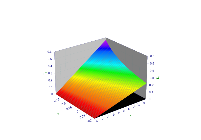
Figure 1: A plot of the critical temperature as a function of $\rho$ and $\gamma$ varying in the range of $-0.5<\gamma<1$

Figure (1) shows the the dependence of $T_{c}$ as a function of $\rho$ and $\gamma$. As we see when $\rho=0$ for different values of $\gamma$ the value of $T_{c}$ is equal to zero, and in the case $\gamma=0$ there is a linear dependency of $T_{c}$ with respect to the varying parameter $\rho$. This is also mentioned in the figure (2) . As we see in the figure(2) when $\rho=0$ the magnitude of $T_{c}$ is equal to zero and when $\rho$ goes higher the $T_{c}$ also goes higher with linear dependency. In the figure (3) we show the dependency of $T_{c}$ with respect to $\gamma$ in the range of $-0.5<\gamma<1$, when $\rho$ is fixed (for example in that case $\rho=10$). With increasing of $\gamma$, the values of $T_{c}$ also increase but not linearity.

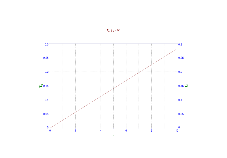
Figure 2: A plot of the $T_{c}$ as a function of $\rho$ ( $\gamma=0$ ). In this plot $\gamma=0$ as we change $\rho$ between 0 and 10. As we see there is linear dependency with respect to parameter $\rho$.

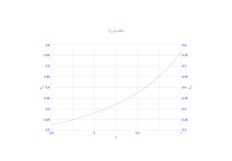
Figure 3: A plot of the $T_{c}$ as a function of $\gamma$ ( $\rho=10$ ). This plot shows how by varying $\gamma$ the values of $T_{c}$ change when $\rho$ is fixed ( for this case $\rho=10$ ).

Noting that in order to remain the temperature $T_{C}$ positive, we must have $h^{\gamma}<\frac{2}{\sqrt{2+\gamma}}$ , and according to the equation(7) we can conclude that($\frac{3}{8}<h<\frac{2}{\sqrt{3}}$) , and it could be reasonable to choose $h=1$ . Near the critical temperature the AdS/CFT dictionary gives the relation below :

$$<\hat{O}_{+}>=\sqrt{2}D_{+}=2\sqrt{2}a=4\sqrt{\frac{2\pi\rho}{\tilde{b}\beta h^{\gamma+3}}}(1-\frac{T}{T_{C}})^{1/2}$$ (57)

We observe that $<\hat{O}_{+}>$ is zero at $T=T_{C}$, the critical point, and condensation occurs for $T<T_{C}$. The continuity of the transition can be checked by computing the free energyHorowitz . We also see a behavior $<\hat{O}_{+}>\propto(T_{C}-T)^{1/2}$ which is a typical mean field theory result for a second order phase transitionGregory .

Figure (4) shows $\langle{\hat{O}}_{+}\rangle$ as a function of temperature normalizing by $T_{c}$ for a variety of values of $\rho$ and $\beta$. Each line in the plot forms the characteristic curve of $\langle{\hat{O}}_{+}\rangle$ condensing at some critical temperature. For simplicity we chose five values of $\rho$ and $\beta$ to display the features of the system and showing how varying $\beta$ and $\rho$ effect the height of $\langle{\hat{O}}_{+}\rangle$. In this figure according to the equation (7), in order to have positive Unruh temperature we must require $\Lambda_{W}<0$.

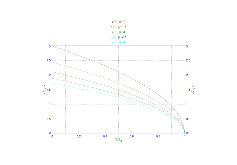
Figure 4: The plot of the condensation as a function of $\frac{T}{T_{c}}$ for a selection of values of $\rho$ and $\beta$. In this plot the value of $\rho$ is fixed ( in this case is equal to one) and the value of $\beta$ from top to down is equal to 1, 1.5, 2, 2.5, 3. As we see the height of $\langle{\hat{O}}_{+}\rangle$ is decreasing as the values of $\beta$ increase, and the condensation occurs when $T<T_{c}$.

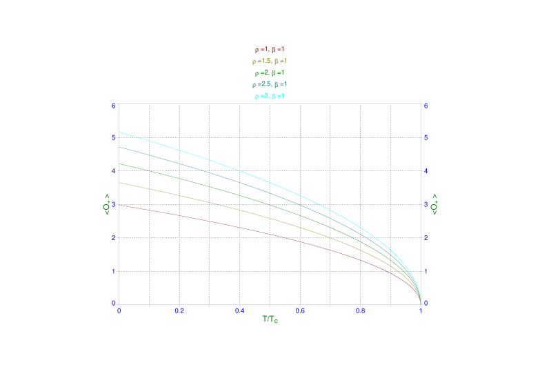
Figure 5: The plot of the condensation as a function of $\frac{T}{T_{c}}$ for a selection of values of $\rho$ and $\beta$. In this plot the value of $\beta$ is fixed ( in this case is equal to one) and the value of $\rho$ from down to top is equal to 1, 1.5, 2, 2.5, 3. As we see the height of $\langle{\hat{O}}_{+}\rangle$ is increasing as the values of $\beta$ increase, and the condensation occurs when $T<T_{c}$.

As we see in figure (4) increasing $\beta$ reduces the value of $\langle{\hat{O}}_{+}\rangle$. We also see that the condensation appears when $T=T_{c}$.

Figure (5) shows that the effect of increasing $\rho$ is to increase the height of these graphs ( $\langle{\hat{O}}_{+}\rangle$ ), in similar way mentioned in figure (4), the condensation happens at $T=T_{c}$.

V Conductivity

In order to compute the electric conductivity in dual CFT , we must solve the Maxwell equation for the fluctuations of the vector potential $A_{x}(r,t)$, located in the bulk. We assume that the time dependence of the field is $e^{-i\omega t}$ and then the field equation of this component reads as:

$$A^{{}^{\prime\prime}}+\left(\frac{f^{{}^{\prime}}}{f}-\frac{(\gamma+1)}{r}\right)A^{{}^{\prime}}+\left[\frac{r^{2\gamma}\omega^{2}}{f^{2}\beta^{2}}-\frac{2\psi^{2}}{f}\right]A=0$$ (58)

which is what mentioned in the papers Gregory ; Gregory2 ; Gregory3 in the special case $\kappa=0$ and $\alpha=\frac{L^{2}}{4}$ where from the metric ansatz we have concluded that $e^{\nu}=\beta r^{-\gamma}$. The causal behavior is obtained with imposing an ingoing wave boundary condition at the horizon bc . The desired asymptotic behavior of the Maxwell field at large distance is

$$A_{x}=A_{x}^{(0)}+\frac{A_{x}^{(1)}}{r}$$ (59)

According to the AdS/CFT dictionary, the dual source and expectation value for the current are given by

$$A_{x}=A_{x}^{(0)},<J_{x}>=A_{x}^{(1)}$$ (60)

Now using Ohm’s law we can obtain the conductivity as

$$\sigma(\omega)=\frac{-iA_{x}^{(1)}}{\omega A_{x}^{(0)}}$$ (61)

Thus we must solve (58) numerically and obtain the imaginary part of the conductivity $\sigma(\omega)$ for a set of parameters $\Lambda_{W}=-2,\beta=-1,\delta=-1$. There is a delta function at $\omega=0$ which appears as $T<T_{C}$, and from the Kramers-Kronig relation we can see that the real part of the conductivity contains a delta function and the imaginary part has a simple pole at $\omega=0$. Thus the superfluid density is of the delta function Horowitz

$$Re(\sigma(\omega))\sim\pi\delta(\omega)$$ (62)

The figure(6) shows the behavior of the real part of conductivity as a function of frequency per temperature for different values of the HL parameter $\alpha$.

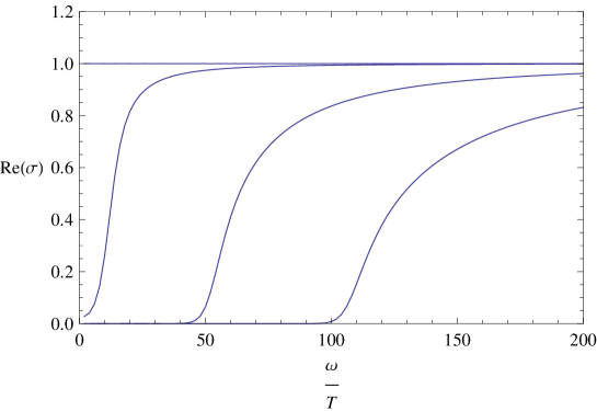
Figure 6: The real part of conductivity $Re(\sigma(\omega))$ as a function of the frequency $\frac{\omega}{T}$ for $O_{1}$ operator

We can solve (58) for operator $O_{2}$ for the former set of the parameters. The result graph has been shown in the figure(7).

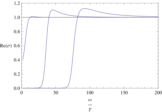
Figure 7: The real part of conductivity $Re(\sigma(\omega))$ as a function of the frequency $\frac{\omega}{T}$ for $O_{2}$ operator

VI Conclusion

In the present work, we have built a holographic model for a non-relativistic system showing superconductivity. We have used a black hole background which comes from the Ho$\check{\textbf{r}}$ava-Lifshitz gravity, and we have studied analytically, holographic superconductors in this new kind of the asymptotic AdS solutions. We also have analytically solved the system in the probe limits, near horizon and asymptotic region. We have found that there is also a critical temperature like the relativistic case, below which a charged condensation field appears by a second order phase transition, and also we have found out below a critical temperature $T_{C}$, the condensation field appears and obtains finite value. We can conclude that as the condensation field becomes heavier, the transition happens more observable. Also the conductivity has been computed and the variation of the critical temperature and conductivity with respect to the parameters of the metric function have been shown. We numerically obtain the conductivity as a function of the frequency for a wide range of the parameters. We show that the Gauss-Bonnet theory in five dimension and Ho$\check{\textbf{r}}$ava-Lifshitz theory in critical exponent $z=3$ and in four dimension share some similar features.

VII Acknowledgment

The authors would like to thank Bin Wang from INPAC (China) for recommending useful references in Gauss-Bonnet superconductors and proposing excellent observations and helpful suggestions resulted in substantial improvements of the presentation and outcomes. Also we thank Betti Hartmann from Jacobs university for suggesting former references for Gauss Bonnet superconductors.

References

- (1) S. A. Hartnoll, C. P. Herzog and G. T. Horowitz, ”Building a holographic superconductor”, Phys. Rev. Lett. 101 (2008) 031601, [arXiv:0803.3295 [hep-th]].
- (2) P. Breitenlohner and D. Z. Freedman, Ann. Phys., 144:249, (1982).
- (3) P. Basu, A. Mukherjee, and H. H. Shieh, Phys.Rev.D79:045010,2009[arXiv:0809.4494 [hep-th]]
- (4) Wen-Yu Wen,”Inhomogeneous magnetic field in AdS/CFT superconductor”, [arXiv: 0805.1550[hep-th]]
- (5) S.S. Gubser, Breaking an Abelian gauge symmetry near a black hole horizon,Phys.Rev.D78:065034,2008[arXiv:0801.2977].
- (6) S.S. Gubser, I.R. Klebanov and A.M. Polyakov, Gauge theory correlators from non-critical string theory, Phys. Lett. B 428 (1998) 105 [hep-th/9802109].
- (7) E. Witten, Anti-de Sitter space and holography, Adv. Theor. Math. Phys. 2 (1998) 253 [hep-th/9802150].
- (8) K. Maeda, and T. Okamura, Phys. Rev. D 78, 106006 (2008).
-
(9)
Maldacena J 1998 Adv. Theor. Math. Phys. 2 253
Witten E 1998 Adv.Theor. Math. Phys. 2 505
Aharony O, Gubser S S, Maldacena J,Ooguri H and Oz Y 2000 Phys. Rep. 323 183 - (10) P. Horava, arXiv:0811.2217 [hep-th].
- (11) P. Horava, JHEP 0903, 020 (2009) [arXiv:0812.4287 [hep-th]].
- (12) P. Horava, Phys. Rev. D 79, 084008 (2009) [arXiv:0901.3775 [hep-th]].
- (13) P. Hořava, arXiv:0902.3657 [hep-th].
- (14) D. Blas, O. Pujolas, S. Sibiryakov, JHEP, 10, (2009), 029.
- (15) A. Kehagias and K. Sfetsos, The black hole and FRW geometries of non-relativistic gravity, Phys. Lett. B 678, 123 (2009) [arXiv:0905.0477 [hep-th]].
- (16) M. R. Setare, D. Momeni, ”Geodesic stability for KS Black hole in Hoava-Lifshitz gravity via Lyapunov exponents ”,Int.J.Theor.Phys.50:106-113,2011 [arXiv:1001.3767v2] [physics.gen-ph].
- (17) H. Lu, J.Mei and C.N. Pope, Phys.Rev.Lett.103:091301,2009[arXiv:0904.1595 [hep-th]]
- (18) Jin-Zhang Tang,[arXiv: 0911.3849[hep-th]]
- (19) Rong-Gen Cai, Li-Ming Cao, and Nobuyoshi Ohta, Phys. Rev. D 80, 024003 (2009).[arXiv: 0904.3670[hep-th]].
- (20) Xian-Hui Ge, Bin Wang, Shao-Feng Wu, Guo-Hong Yang, ”Analytical study on holographic superconductors in external magnetic field”,JHEP08(2010)108 arXiv:1002.4901; Qiyuan Pan, Bin Wang, Eleftherios Papantonopoulos, J. Oliveira, A. Pavan, ”Holographic Superconductors with various condensates in Einstein-Gauss-Bonnet gravity”,Phys.Rev.D81:106007,2010 [arXiv:0912.2475]; Liu, Yunqi; Pan, Qiyuan; Wang, Bin; Cai, Rong-Gen , ” Dynamical perturbations and critical phenomena in Gauss-Bonnet AdS black holes ”, Physics Letters B, Volume 693, Issue 3, p. 343-350; Qiyuan Pan, Bin Wang , ”General holographic superconductor models with backreactions ”, [arXiv: arXiv:1101.0222v1 [hep-th]]; Pan, Qiyuan; Wang, Bin , ”General holographic superconductor models with Gauss-Bonnet corrections”, Physics Letters B, Volume 693, Issue 2, p. 159-165
- (21) Yves Brihaye ; Betti Hartmann,”Holographic Superconductors in 3+1 dimensions away from the probe limit”, Phys.Rev. D81 (2010) 126008 ,[arXiv:1003.5130 [hep-th]]
- (22) Jiliang Jing, Liancheng Wang, and Songbai Chen,[arXiv: 1001.1472[hep-th]]
- (23) R. Arnowitt, S. Deser and C. W. Misner, in Gravitation: an introduction to current research (Chap. 7). Edited by Louis Witten. John Wiley and Sons Inc., New York, London, (1962).
- (24) Thomas P. Sotiriou, Matt Visser, Silke Weinfurtner, Phenomenologically viable Lorentz-violating quantum gravity , Phys.Rev.Lett.102:251601,2009, arXiv:0904.4464 [hep-th]; Quantum gravity without Lorentz invariance, arXiv:0905.2798 [hep-th].
- (25) G. W. Gibbons and S. W. Hawking, Commun. Math. Phys. 66 (1979),291.
- (26) R. A. Konoplya,”Entropic force, holography and thermodynamics for static space-times”,Eur.Phys.J.C69:555-562,2010[arXiv:1002.2818v2 [hep-th] ]
- (27) S. A. Hartnoll, C. P. Herzog and G. T. Horowitz, ” holographic superconductors”, JHEP12 (2008) 015, [arXiv:0803.3295 [hep-th]].
- (28) L. J. Romans, Nucl. Phys. B 383 (1992), 395, [hep-th/9203018].
- (29) T. Albash and C. V. Johnson, JHEP 09 (2008), 121.
- (30) R. G. Cai and H. Q. Zhang, ”Holographic Superconductors with Hovrava-Lifshitz Black Holes”,Phys.Rev.D81:066003,2010 [hep-th/0911.4867].
- (31) P. Kanti and J. March-Russell, Phys. Rev. D 67, 104019 (2003); R. Gregory, S. Kanno, and J. Soda, JHEP 0910, 010 (2009).
- (32) I. R. Klebanov and E. Witten, Nucl. Phys. B 556, 89 (1999),[hep-th/9905104].
- (33) R. Gregory, S. Kannoa and J. Sodab, ”Holographic superconductors with higher curvature corrections”, JHEP 10 (2009) 010.
- (34) R. Gregory, S. Kannoa and J. Sodab, ”Holographic superconductors with Gauss- bonnet Gravity”, arxive:1012.1558[hep-th].
- (35) L. Baraclay, R. Gregory, S. Kannoa and P. Sutcliffe, ”Gauss- bonnet Holographic superconductors ”,JHEP 1012:029,2010 [arxiv:1009.1991[hep-th]].
- (36) G. T. Horowitz and M. M. Roberts,Phys. Rev. 78,126008(2008)[arXive:0810.1563[hep-th]].
- (37) K. Skenderis,Class. Quant. Grav. 19,5849(2002)[arXive:0209067[hep-th]].
- (38) D. T. Son and A. O. Starinets, JHEP 09, (2002) 042