Analysis of return distributions in the coherent noise model

Abstract

The return distributions of the coherent noise model are studied for the system size independent case. It is shown that, in this case, these distributions are in the shape of $q$-Gaussians, which are the standard distributions obtained in nonextensive statistical mechanics. Moreover, an exact relation connecting the exponent $\tau$ of avalanche size distribution and the $q$ value of appropriate $q$-Gaussian has been obtained as $q=(\tau+2)/\tau$. Making use of this relation one can easily determine the $q$ parameter values of the appropriate $q$-Gaussians a priori from one of the well-known exponents of the system. Since the coherent noise model has the advantage of producing different $\tau$ values by varying a model parameter $\sigma$, clear numerical evidences on the validity of the proposed relation have been achieved for different cases. Finally, the effect of the system size has also been analyzed and an analytical expression has been proposed, which is corroborated by the numerical results.

1 Introduction

Throughout the last two decades the interest in extended dynamical systems has experienced a steady increase. These systems exhibit avalanches of activity whose size distributions are of power-law type. Although there is not a unique nor unified theory which totally explains all the features of these complex systems, there exist several known mechanisms producing power-law behavior. One of the most popular and well-studied mechanisms is that of self-organized criticality (SOC) introduced by Bak, Tang and Wiesenfeld [1]. Many physical systems and models have shown to exhibit SOC [2]. The most important feature of all these systems is that the entire system is under the influence of a small local driving force, which makes the system evolve towards a critical stationary state having no characteristic spatiotemporal scale, without invoking a fine-tuning of any parameter. On the other hand, SOC is not the only mechanism causing power-law correlations that appear in a nonequilibrium steady state. Another simple and robust mechanism exhibiting the same feature in the absence of criticality is the coherent noise model (CNM) [3, 4]. The CNM is based on the notion of an external stress acting coherently onto all agents of the system without having any direct interaction with agents. Therefore, the model does not exhibit criticality, but it still gives a power-law distribution of event sizes (avalanches).

Recently, it was presented an analysis method to interpret SOC behavior in the limited number of earthquakes from the World and California catalogs by making use of the return distributions (i.e., distributions of the avalanche size differences at subsequent time steps) [5]. In their work Caruso et al obtained the first evidence that the return distributions seem to have the form of $q$-Gaussians, standard distributions appearing naturally in the context of nonextensive statistical mechanics [6, 7]. Based on the assumption that there is no correlation between the size of two events, they were also able to propose a relation between the exponent $\tau$ of the avalanche size distribution and the $q$ value of the appropriate $q$-Gaussian as

$$q=e^{1.19\;\tau^{-0.795}}\;\;,$$ (1)

which is rather important since it makes the $q$ parameter determined a priori and therefore it acquits $q$ of becoming a fitting parameter. The only little drawback of their work was that the number of data taken from the catalogs is not sufficiently large to obtain a very precise $\tau$ exponent and also clear return distributions with well-defined tails (which is important in order to verify how good the distribution approaches a $q$-Gaussian). Consequently, Eq. (1) could not be rigorously tested until a very recent effort by Bakar and Tirnakli in [8], where the same analysis was made using a simple SOC model known as the Ehrenfest dog-flea model in the literature [9] (see also [10, 11]). Thanks to the simplicity of the dog-flea model, it was possible to achieve extensive simulations with very large system sizes (up to $10^{7}$) and also very large number of data elements (up to $2\times 10^{9}$). Accordingly, from these extensive simulations, it was obtained a value of $\tau=1.517$, which is in accordance with the “mean-field” exponent $3/2$ determined in several problems [12, 13, 14]. Thence the $q$ value of return distributions was deduced a priori from Eq. (1).

In this work, we plod along this way by setting forth the following points: (i) first, we will obtain an exact relation between $\tau$ exponent of the avalanche size distribution and the $q$ value of the appropriate $q$-Gaussian without resorting to any assumption and compare it to Caruso et al relation given in Eq. (1), (ii) since the CNM has the advantage of producing different $\tau$ values by varying a model parameter $\sigma$ , we now have the opportunity to test the validity of our exact relation (and also the Caruso et al relation) not only for one case but for various cases, (iii) since the corresponding return distributions are expected to converge to the $q$-Gaussian as the system size goes to infinity, the effect of finite system size is also important and we shall try to analyze this effect proposing an analytical expression, (iv) and finally since this model is not a SOC model, our results also give us the possibility of checking the generality of this behavior observed so far in SOC models.

2 The coherent noise model

Let us start by introducing the CNM. It is a system of $N$ agents, each one having a threshold $x_{i}$ against an external stress $\eta$. The threshold levels and the external stress are randomly chosen from probability distributions $p_{thresh}(x)$ and $p_{stress}(\eta)$, respectively. Throughout our simulations we use the exponential distribution for the external stress, namely, $p_{stress}(\eta)=(1/\sigma)\exp(-\eta/\sigma)$ and the uniform distribution ($0\leq x\leq 1$) for $p_{thresh}(x)$. The dynamics of the model is very simple: (i) generate a random stress $\eta$ from $p_{stress}(\eta)$ and replace all agents with $x_{i}\leq\eta$ by new agents with new threshold drawn from $p_{thresh}(x)$, (ii) choose a small fraction $f$ of $N$ agents and assign them new thresholds drawn again from $p_{thresh}(x)$, (iii) repeat the first step for the next time step. The model can be described in the form of a two step-master equation that we present in the appendix. The number of agents replaced in the first step of the dynamics determines the event size $s$ for this model. Although the CNM has been introduced for analyzing biological extinctions [3], it has then been adopted as a very simple mean field model for earthquakes even though no geometric configuration space is introduced in the model [4]. It is shown that the model obeys the Omori law for the temporal decay pattern of aftershocks [15], exhibits aging phenomena [16] and power-law sensitivity to initial conditions [17].

3 Avalanche Size and Return Distributions

3.1 Size independent case

As pointed out in [4], there is advantage in choosing the uniform distribution ($0\leq x\leq 1$) for the thresholds of the CNM agents seeing that the model can be simulated in the $N\rightarrow\infty$ limit using a fast algorithm which acts directly on the threshold distribution instead of acting on the agents of the system. This enables us to obtain the avalanche size distribution $P(s)$ of the model as being independent of the system size. The distribution $P(s)$ is expected to be a power-law over many decades until the $s$ values reach a particular point $s\sim\sigma$, thereafter it falls off exponentially. From our point of view this is rather important since it means that if we measure the avalanche size exponent $\tau$ using the region $s<\sigma$, then we must use this $\tau$ value to predict a priori the $q$ value of the $q$-Gaussian that the return distribution is expected to converge in the entire region without any deterioration (not only in the central part but also in the tails). The results obtained for the avalanche size distributions of three representative cases with $\sigma=0.01$, $\sigma=0.05$ and $\sigma=0.065$ are given in the left column of Fig. 1.

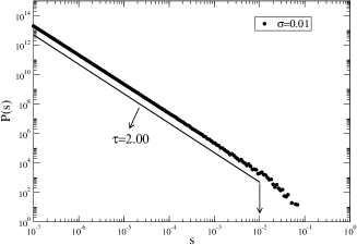
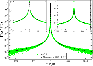
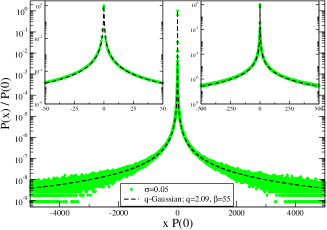
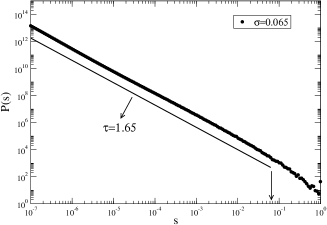
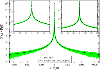
Figure 1: Left column: Avalanche size distributions of three representative values of $\sigma$. For each case, the $\tau$ value is calculated using standard regression method for the region $s<\sigma$. Right column: Return distributions for the same three cases. Two zooms of the central part are given in the insets for better visualization. For each case, $f=10^{-7}$ and $2\times 10^{9}$ experiments are generated.

Since each case with different $\sigma$ values has a different size exponent $\tau$, this allows us to check the validity of Caruso et al relation given in Eq. (1) or any other equation relating $\tau$ values to the $q$ values of the appropriate $q$-Gaussians. From the master-equation of the CNM is theoretically possible to compute the probability of $s$ and bringing to bear standard techniques [13] to obtain the return distribution. However, its level of complexity turns out the solution almost analytically impossible or its (asymptotic) behavior deeply unclear as it happens in several other problems of this class [18]. Regardless, we are in the position where we can propose an exact relation for the return distribution $P\left(\Delta s\right)$ bringing into play no other assumption than the distribution of avalanche sizes, where $\Delta s$ is the difference between two consecutive event sizes, i.e., $\Delta s=s(t+1)-s(t)$. Let us mathematically define the avalanche size distribution,

$$p(s)\propto\left(\varepsilon+s\right)^{-\tau},\qquad\left(\tau>1\right),$$ (2)

with $\varepsilon$ being a constant value describing the asymptotic limit $s\rightarrow 0$. The process of avalanches is completely Markovian (independent) and therefore the probability of the difference of sizes $\Delta s$ is

$$P\left(\Delta s\right) = \int_{0}^{\infty}\int_{0}^{\infty}p(s)\,p(s^{\prime})\,\delta\left(\Delta s-\left(s-s^{\prime}\right)\right)\,ds^{\prime}\,ds.$$

$$= \int_{0}^{\infty}\left(\varepsilon+s\right)^{-\tau}\left(\varepsilon+\Delta s+s\right)^{-\tau}\,\Theta\left(\Delta s+s\right)\,ds,$$

where $\Theta(\ldots)$ is the Heaviside step function and $s^{\prime}$ denotes the previous avalanche size. Making use of [19] and attending to the symmetric nature of $P\left(\Delta s\right)$ we can explicit the negative branch,

$$P\left(\Delta s\right)=\left|\Delta s\right|^{1-2\,\tau}\left(B\left[\frac{\varepsilon}{\Delta s},1-\tau,1-\tau\right]\left(-1\right)^{\tau}+\mathcal{C}\left(\tau\right)\right),$$ (3)

where $\mathcal{C}\left(\tau\right)$ is a coefficient only depending on $\tau$ and related to the convolution of very large values of $s$ with very large values of $-s^{\prime}$ yielding a $\left|\Delta s\right|^{1-2\,\tau}$ dependence . Thus, the distribution is mainly described by the product of the isolated factor by the incomplete Beta function $B[\ldots]$. Applying the asymptotic behavior $x\rightarrow 0$ of $B[x,a,b]$ [20] we finally get,

$$P\left(\Delta s\right)\sim\left|\Delta s\right|^{-\,\tau},\qquad\left(\Delta s\gg 1\right).$$

Taking note of the $q$-Gaussian distribution,

$$P(\Delta s)=P(0)\left[1+{\bar{\beta}}(q-1)\Delta s^{2}\right]^{1/(1-q)},$$ (4)

we straightforwardly obtain

$$q=\frac{\tau+2}{\tau}.$$ (5)

This relation is slightly different from the approximate relation presented in [5] as can be seen in Fig. 2. For $\tau\rightarrow\infty$, both relations approach $q=1$ and they are almost identical except in the region where $\tau$ values are smaller than $1.5$. Moreover, only the relation (5) correctly achieves $q=3$ value when $\tau=1$. These values define the limits of the domain of each parameter so that the distributions (2) and (4) are normalizable. The approximate relation Eq. (1) does not fulfill this condition as $q\left(\tau=1\right)>3$. It should be noted that, since this discrepancy is only meaningful for $\tau<1.5$, the approximate relation predicts the $q$ values with a $|0.01|$ difference from the exact one, which are also acceptable for all the cases we present.

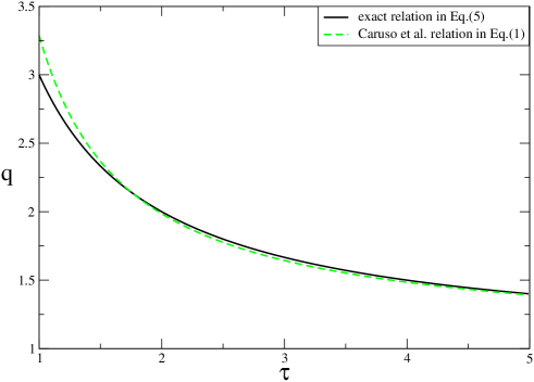
Figure 2: Comparison of our exact relation (Eq. (5)) with that of Caruso et al (Eq. (1)).

We are now ready to proceed analyzing the return distributions. The centered returns are given in terms of variable $x$

$$x=\Delta s-\left\langle\Delta s\right\rangle\;\;,$$ (6)

where $\left\langle...\right\rangle$ represents the mean value of a given data set. As can be seen from the right column of Fig. 1, in our simulations we generated the return distributions of the three representative cases of the CNM in order to check the validity of the relation (5). In each case, an extremely large number of events ($2\times 10^{9}$) has been used to build the numerical distribution, namely, the central part and tails. It is clear that the return distribution (green dots) can by no means be approached by a Gaussian. They actually exhibit fat tails which agree with $q$-Gaussians Eq. (4) where ${\bar{\beta}}$ characterizes the width of the distribution and $q$ is the parameter which should be determined directly from Eq. (5) a priori and therefore is no longer a fitting parameter. In each panel on the right column of Fig. 1, the dashed black lines represent the appropriate $q$-Gaussian with the $q$ value obtained from Eq. (5). Perfect agreement with the data can be easily appreciated not only for the tails but also for the intermediate and the very central part as it is demonstrated in the insets.

3.2 Size dependent case

Although we might think that the size independent (i.e., infinite size) case would be enough for such an analysis, we believe that it is still instructive to look also at the size dependent case at least from two different perspectives: (i) we can check how the size of the system affects the shape of the return distributions and whether the tendency is consistent with the infinite size case as the size of the system increases, (ii) unlike the CNM, generic size independent cases cannot be achieved for such systems and thus the only possibility is to always analyze the size dependent case.

It is very easy to implement the size dependent algorithm for the CNM. We just need to apply the previously described steps of the dynamics to a system of $N$ agents. As $N$ increases, this algorithm clearly slows down and for the same number of events ($10^{9}$) the larger value of $N$ that we can simulate in a reasonable time is $20000$. In Fig. 3(a) the behavior of the avalanche size distribution is given for $\sigma=0.05$ case for various $N$ values. It is clearly seen that the power-law regime is always followed by an exponential decay of all the curves and this decay is postponed to larger sizes as $N$ increases. For each $N$ case, we estimate the $\tau$ value using the standard regression method in the region before the exponential decay (we determine the size of this interval by looking at the regression coefficient to become always more than 0.9997 in each case). Therefore, we should expect that the exponential decay part would tamper with the $q$-Gaussian behavior of the return distributions and this meddling must diminish as $N$ gets larger and larger, which is in fact observed in Fig. 3(b) for the return distributions of four representative $N$ values. When $N$ values are very small, avalanche size distribution has a very short power-law region and the exponential decay part dominates, which simply causes the return distributions to deviate immediately from the $q$-Gaussian shape. As $N$ increases, return distributions start approaching the thermodynamic limit (dotted black line), which is a full $q$-Gaussian with $q=2.09$, yielding better and better from the central part to the tails, i.e., as the expected scale-free regime sets in.

In order to explain this gradual approach to $q$-Gaussians when finite-size effects are present, let us try to develop a simple mathematical model by considering the differential equation

$$\frac{dy}{d(x^{2})}=-a_{r}y^{r}-(a_{q}-a_{r})y^{q}\;\;\;\;(a_{q}\geq a_{r}\geq 0;\,q>r;\,y(0)=1)\,.$$ (7)

This equation has very interesting and different solutions depending on the choice of $r$ and $q$ values (see refs.[7, 21, 22]), but for our purpose, let us concentrate on case $r=1$ and $q>1$, whose solution is given by

$$y=\left[1-\frac{a_{q}}{a_{1}}+\frac{a_{q}}{a_{1}}\,e^{(q-1)a_{1}\,x^{2}}\right]^{1/(1-q)}\,.$$ (8)

If $a_{1}=0$, then the solution coincides with the $q$-Gaussian, whereas if $a_{q}=a_{1}$ (which means that $q=1$), the solution turns out to be the Gaussian. On the other hand, between these two extremes, namely if $a_{q}>a_{1}>0$ and $q>1$, we obtain a crossover between them. Specifically, for $(q-1)\,a_{1}\,x^{2}\ll 1$, Eq. (8) approaches a $q$-Gaussian, $y\sim\left[1-(1-q)\,a_{q}\,x^{2}\right]^{1/(1-q)}$. Our results, which are depicted in Fig. 3, show that the small values of $a_{1}$ imply that the $q$-Gaussian form is valid up to rather large values of $x$. On the other hand, for $(q-1)\,a_{1}\,x^{2}\gg 1$, the exponential outnumbers the remaining terms leading to the Gaussian behaviour,

$$y\asymp\left(\frac{a_{q}}{a_{1}}\right)^{1/(1-q)}\exp\left(-a_{1}\,x^{2}\right).$$

The approximate dependence of Eq. (8) can thus be split into different regions defined by three values of $x$. Namely the first value is

$$x_{a}\sim\sqrt{\frac{W\left[-\frac{a_{1}}{a_{q}}\right]}{a_{1}(1-q)}},$$

($W\left[\ldots\right]$ is the Lambert $W$ function [20]) whence the curve assumes a power-law dependence described by the exponent $2/(q-1)$ that persists up to

$$x_{b}\sim\sqrt{\frac{\ln 2}{a_{1}(q-1)}},$$

when the it starts being perturbed by the Gaussian dependence. Last, there is the final convergence to the Gaussian functional form which occurs at

$$x_{c}\sim\sqrt{\frac{\ln\left(1-\frac{a_{1}}{a_{q}}+\frac{a_{q}}{a_{1}}\right)}{a_{1}\,(q-1)}}.$$

This crossover seems to coincide with the behavior of the return distributions of the $N$ dependent cases as plotted with dashed black lines on top of each curve in Fig. 3(b). This behavior simply reveals that the longer the power-law regime persists for avalanche size distribution, the better the appropriate $q$-Gaussian dominates in the return distribution. Finally, as $N\rightarrow\infty$, the power-law regime prevails for the avalanche size distribution giving forth a return distribution following the appropriate $q$-Gaussian for the entire region.

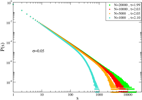
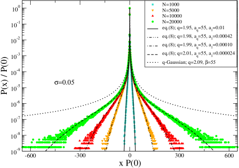
Figure 3: (a) Avalanche size distributions for $N$ dependent case. (b) Corresponding return distributions of the same $N$ values.

4 Conclusion

In this work, we have studied the behavior of the return distributions for the CNM by directly simulating the size independent case. By means of extensive simulations, it is clearly shown that these distributions converge to $q$-Gaussians with appropriate $q$ values which are deduced a priori from the exact relation (5) that we developed here. It is worth noting that although the $q$-Gaussian description is actually an analytical approximation the result provides for an understandable depiction of the distribution, which hardly occurs when we keep a special functions representation, with no fundamental accuracy lost. This relation makes the $q$ parameter be related to one of the well-known exponents (avalanche size exponent $\tau$) of such complex systems and therefore it rescues $q$ from being a fitting parameter in this analysis. Moreover, since the model parameter $\sigma$ allows us to obtain different $\tau$ values, we were able to check this behavior for various cases. These results clearly imply that the observed behavior is not restricted to self-organized critical models, but instead it seems to be a rather generic feature presented by many complex systems which exhibit asymptotic power-law distribution of avalanche sizes.

We have also investigated the finite-size effect by simulating directly the model dynamics and found that the convergence to appropriate $q$-Gaussian starts from the central part and gradually evolves towards the tails as the system size increases. This is in complete agreement with the gradual extension of the power-law regime in the avalanche size distribution before the appearance of the exponential decay due to finite-size of the system. These results corroborate the analysis of size independent case since it is clearly seen that, as $N\rightarrow\infty$, curves of return distributions for size dependent case converge to the one comes from the size independent case.

Finally it should be noted that, since it is generically extremely difficult (if not impossible) to achieve the size independent case for such complex systems, the size dependent case has its particular importance. Therefore, although the return distributions appear to be $q$-Gaussians for the entire region in the thermodynamic limit, we have tried to propose a mathematical model in order to explain the behavior of return distributions for the size dependent case.

Acknowlegment

We are indebted to M E J Newman for providing us his fast (size independent) code for the coherent noise model and C Anteneodo for interesting discussions about passage problems and related references. This work has been supported by TUBITAK (Turkish Agency) under the Research Project number 104T148 and by Ege University under the Research Project number 2009FEN027.

Appendix A The CNM master equation

The dynamics of the CNM can be described according to the probability of having $n$ agents in the system that at time $t$ present a critical value up to $x$, $P_{n}\left(x,t\right)$. In conformity with step 1 we can write the master-equation,

$$P_{n}\left(x,t\right) = P_{n}\left(x,t-1\right)W_{n\rightarrow n}+\sum\limits_{l=1}^{n}P_{n-l}\left(x,t-1\right)W_{n-l\rightarrow n}$$ (9)

$$+\sum\limits_{l=1}^{N-n}P_{n+l}\left(x,t-1\right)W_{n+l\rightarrow n}-\sum\limits_{l=1}^{n}P_{n}\left(x,t-1\right)W_{n\rightarrow n-l}$$

$$-\sum\limits_{l=1}^{N-n}P_{n}\left(x,t-1\right)W_{n\rightarrow n+l}$$

with the probability transitions $W$ given by

$$W_{n\rightarrow n}=x^{n}\,F^{\prime}\left(x\right)+\sum_{m=1}^{n}\int_{0}^{x}x^{m}\frac{m}{n}\,p_{thresh}\left(\eta\right)\,\delta\left(m-M_{x,\eta}\right)d\eta,$$ (10)

where the first term on the rhs comes from the case $\eta\geq x$ and the second one otherwise. The inverse cumulative probability $F^{\prime}\left(x\right)\equiv 1-F\left(x\right)=1-\int_{0}^{x}p_{thresh}\left(z\right)\,dz$  and $M_{x,\eta}\equiv\sum_{i=1}^{N}\Theta\left[\eta-x_{i}\left(t\right)\right]\Theta\left[x-\eta\right]$ means the number of agents with critical value below $x$ and $\eta$. The following elements are

$$W_{n-l\rightarrow n}=W_{n\rightarrow n+l}=0,$$ (11)

$$W_{n+l\rightarrow n}=\left(\begin{array}[]{c}n+l\\ n\end{array}\right)x^{n}\left(1-x\right)^{l}\,F^{\prime}\left(x\right)+$$ (14)

$$\sum_{m\geq l}^{n+l}\int_{0}^{x}\left(\begin{array}[]{c}m\\ m-l\end{array}\right)x^{m-l}\left(1-x\right)^{l}\frac{m}{n+l}\,p_{thresh}\left(\eta\right)\,\delta\left(m-M_{x,\eta}\right)d\eta,$$ (17)

$$W_{n\rightarrow n-l}=\left(\begin{array}[]{c}n\\ n-l\end{array}\right)x^{n-l}\left(1-x\right)^{l}\,F^{\prime}\left(x\right)+$$ (20)

$$\sum_{m\geq l}^{n}\int_{0}^{x}\left(\begin{array}[]{c}m\\ m-l\end{array}\right)x^{m-l}\left(1-x\right)^{l}\frac{m}{n}\,p_{thresh}\left(\eta\right)\,\delta\left(m-M_{x,\eta}\right)d\eta.$$ (23)

This corresponds to a matrix with vanishing elements below the diagonal. From these relations is then possible to spell out the occurrence of an avalanche of size $s$

$$P\left(s\right)=\left\{\begin{array}[]{ccc}\sum_{n=0}^{N}\int_{0}^{1}\frac{dP_{n}\left(x,t-1\right)}{dx}\,W_{n\rightarrow n}\,dx&\Leftarrow&s=0\\ &&\\ \begin{array}[]{c}\sum_{n=0}^{N-s}\int_{0}^{1}\frac{dP_{n+s}\left(x,t-1\right)}{dx}\,W_{n+s\rightarrow n}\,dx+\\ \sum_{n=s}^{N}\int_{0}^{1}\frac{dP_{n}\left(x,t-1\right)}{dx}\,W_{n\rightarrow n-s}\,dx\end{array}&\Leftarrow&s\neq 0\end{array}\right.,$$ (24)

which is numerically well described by the power-law (2) with a small value of $\varepsilon$.

Regarding step 2 the master equation is abstractly pretty much the same,

$$P_{n}\left(x,t+1\right)= P_{n}\left(x,t\right)W_{n\rightarrow n}+\sum\limits_{l=1}^{n}P_{n-l}\left(x,t\right)W_{n-l\rightarrow n}+\sum\limits_{l=1}^{N-n}P_{n+l}\left(x,t\right)W_{n+l\rightarrow n}$$ (25)

$$-\sum\limits_{l=1}^{n}P_{n}\left(x,t\right)W_{n\rightarrow n-l}-\sum\limits_{l=1}^{N-n}P_{n}\left(x,t\right)W_{n\rightarrow n+l}\,,$$

with the probability transition matrix is given by

$$W_{n\rightarrow n}=\int_{0}^{1}\left(\begin{array}[]{c}n\\ \rho f\,N\end{array}\right)\left(\begin{array}[]{c}N-n\\ \left(1-\rho\right)f\,N\end{array}\right)\left(\begin{array}[]{c}f\,N\\ \rho f\,N\end{array}\right)\left(x\frac{n}{N}\right)^{\rho\,f\,N}\,\times$$ (32)

$$\left[\left(1-x\right)\left(1-\frac{n}{N}\right)\right]^{\left(1-\rho\right)fN}\Theta\left[n-\rho fN\right]\;\Theta\left[N-n-\left(1-\rho\right)fN\right]\,d\rho$$ (33)

where $\rho$ is used to define the subfraction of agents, $\rho fN$, whose critical value before updating was less than $x$.

$$W_{n-l\rightarrow n}=\int_{0}^{1}\left(\begin{array}[]{c}n-l\\ \rho f\,N\end{array}\right)\left(\begin{array}[]{c}N-\left(n-l\right)\\ \left(1-\rho\right)f\,N\end{array}\right)\left(\begin{array}[]{c}f\,N\\ \rho f\,N+l\end{array}\right)\times$$ (40)

$$\left(\frac{n-l}{N}\right)^{\rho\,f\,N}\left(1-\frac{n-l}{N}\right)^{\left(1-\rho\right)fN}x^{\rho\,f\,N+l}\left(1-x\right)^{\left(1-\rho\right)fN-l}\times$$

$$\Theta\left[n-l-\rho fN\right]\,\,\Theta\left[N-\left(n-l\right)-\left(1-\rho\right)fN\right]\,\,d\rho$$ (41)

$$W_{n+l\rightarrow n}=\int_{0}^{1}\left(\begin{array}[]{c}n+l\\ \rho f\,N\end{array}\right)\left(\begin{array}[]{c}N-\left(n+l\right)\\ \left(1-\rho\right)f\,N\end{array}\right)\left(\begin{array}[]{c}f\,N\\ \rho f\,N-l\end{array}\right)\times$$ (48)

$$\left(\frac{n+l}{N}\right)^{\rho\,f\,N}\left(1-\frac{n+l}{N}\right)^{\left(1-\rho\right)fN}x^{\rho\,f\,N-l}\left(1-x\right)^{\left(1-\rho\right)fN+l}\times$$

$$\Theta\left[n+l-\rho fN\right]\,\,\Theta\left[N-\left(n+l\right)-\left(1-\rho\right)fN\right]\,\,d\rho$$ (49)

$$W_{n\rightarrow n-l}=\int_{0}^{1}\left(\begin{array}[]{c}n\\ \rho f\,N\end{array}\right)\left(\begin{array}[]{c}N-n\\ \left(1-\rho\right)f\,N\end{array}\right)\left(\begin{array}[]{c}f\,N\\ \rho f\,N-l\end{array}\right)\times$$ (56)

$$\left(\frac{n}{N}\right)^{\rho\,f\,N}\left(1-\frac{n}{N}\right)^{\left(1-\rho\right)fN}x^{\rho\,f\,N-l}\left(1-x\right)^{\left(1-\rho\right)fN+l}\,\times$$

$$\Theta\left[n-\rho fN\right]\,\,\Theta\left[N-n-\left(1-\rho\right)fN\right]\,d\rho;$$ (57)

$$W_{n\rightarrow n+l}=\int_{0}^{1}\left(\begin{array}[]{c}n\\ \rho f\,N\end{array}\right)\left(\begin{array}[]{c}N-n\\ \left(1-\rho\right)f\,N\end{array}\right)\left(\begin{array}[]{c}f\,N\\ \rho f\,N+l\end{array}\right)\times$$ (64)

$$\left(\frac{n}{N}\right)^{\rho\,f\,N}\left(1-\frac{n}{N}\right)^{\left(1-\rho\right)fN}x^{\rho\,f\,N+l}\left(1-x\right)^{fN\left(1-\rho\right)-l}\times$$

$$\Theta\left[n-\rho fN\right]\,\,\Theta\left[N-n-\left(1-\rho\right)fN\right]\,d\rho.$$ (65)

References

- [1] Bak P, Tang C and Wiesenfeld K 1987 Phys. Rev. Lett. 59 381
- [2] Jensen H J 1988 Self-Organized Criticality: Emergent Complex Behavior in Physical and Biological Systems (Cambridge: Cambridge University Press); Bak P, How Nature Works: The Science of Self-organized Criticality (New York: Copernicus)
- [3] Newman M E J 1996 Proc. R. Soc. London, Ser. B 263 1605
- [4] Newman M E J and Sneppen K 1996 Phys. Rev. E 54 6226; Sneppen K and Newman M E J 1997 Physica D 110 209
- [5] Caruso F, Pluchino A, Latora V, Vinciguerra S and Rapisarda A 2007 Phys. Rev. E 75 055101(R)
- [6] Tsallis C 1988 J. Stat. Phys. 52 479; Curado E M F and Tsallis C 1991 J. Phys. A 24 L69; Corrigenda: 1991 24 3187 and 1992 25 1019; Tsallis C, Mendes R S and Plastino A R 1998 Physica A 261 534
- [7] Tsallis C 2009 Introduction to Nonextensive Statistical Mechanics - Approaching a Complex World (New York:Springer)
- [8] Bakar B and Tirnakli U 2009 Phys. Rev. E 79 040103(R)
- [9] Ehrenfest P and Ehrenfest T 1907 Phys. Z. 8 311
- [10] Nagler J, Hauert C and Schuster H G 1999 Phys. Rev. E 60 2706
- [11] Hauert C, Nagler J and Schuster H G 2004 J. Stat. Phys. 116 1453
- [12] Kac M 1947 Amer. Math. Month. 54 369
- [13] Redner S 2001 A guide to first-passage processes (Cambridge: Cambridge University Press); Fisher M E 1984 J. Stat. Phys. 34 667
- [14] Anteneodo C 2009 Phys. Rev. E 80 041131
- [15] Wilke C, Altmeyer S and Martinetz T 1998 Physica D 120 401
- [16] Tirnakli U and Abe S 2004 Phys. Rev. E 70 056120
- [17] Ergun E and Tirnakli U 2005 Eur. Phys. J. B 46 377
- [18] Anteneodo C and Duarte Queirós S M 2009 unpublished
- [19] Gradshteyn I S and Ryzhik I M 1980 Table of Integrals, Series, and Products (New York: Academic Press)
- [20] http://functions.wolfram.com
- [21] Tsallis C, Bemski G and Mendes R S 1999 Phys. Lett. A 257 93
- [22] Tsallis C and Tirnakli U 2010 J. Phys.: Conf. Ser. 201 012001