ON THE QUANTIZED RELATIVISTIC MEAN FIELD THEORY
FOR NUCLEAR MATTER

Abstract

We propose a quantization procedure for the nucleon-scalar meson system, in which an arbitrary mean scalar meson field $\phi$ is introduced. The equivalence of this procedure with the usual ones is proven for any given value of $\phi$. By use of this procedure, the scalar meson field in the Walecka’s RMFT and in Chin’s RHA are quantized around the mean field. Its corrections on these theories are considered by perturbation up to the second order. The arbitrariness of $\phi$ makes us free to fix it at any stage in the calculation. When we fix it in the way of Walecka’s RMFT, the quantum corrections are big, and the result does not converge. When we fix it in the way of Chin’s RHA, the quantum correction is negligibly small, and the convergence is excellent. It shows that RHA covers the leading part of quantum field theory for nuclear systems and is an excellent zeroth order approximation for further quantum corrections, while the Walecka’s RMFT does not. We suggest to fix the parameter $\phi$ at the end of the whole calculation by minimizing the total energy per-nucleon for the nuclear matter or the total energy for the finite nucleus, to make the quantized relativistic mean field theory (QRMFT) a variational method.

Key words:     Relativistic mean field theory, quantum corrections, quantization around a classical value

PACS number(s):03.65.Ca, 21.60.-n, 21.65.-f

I Introduction

Relativistic Mean Field Theory (RMFT) is a fruitful and widely used theory in nuclear physicsl ; w74 ; c2 ; sw ; w ; fps ; c1 ; bs83 ; z2 ; r1 ; r2 ; b ; z3 ; g . Its agreement with observational data is impressive. It seems to show that the nuclear data under certain energy scale, say several hundred MeV, may be roughly understood by hadron field theory. Of course, it should be a quantum theory of fields. But in RMFT, meson field operators are replaced by their expectation values, which are considered as classical. RMFT is therefore semi-classical. A meaningful RMFT must be followed by quantum corrections due to meson field quantization, and the correction should not qualitatively change its agreement with observational data. In this case, one may realize a quantum hadron field theory for nuclear systems under certain energy scale, with RMFT to be the zeroth order contribution, and calculate quantum corrections by perturbation.

Quantum hadron field theory has already been developed for nuclear physics in the usual loop expansion formalisml ; w74 ; c2 ; sw ; w ; fps , in which the mean meson field is the contribution of the tadpole diagrams. The attachment of nucleon loops (tadpole heads) on a nucleon line by the scalar meson lines (tadpole tails) changes the nucleon mass. Since the tadpole head itself is also formed by a nucleon line, the RMFT calculation for a nuclear system means an infinite series of attachments of tadpoles on tadpoles. In this sense, RMFT is non-perturbative, like the method of self-consistent field widely used in quantum mechanics. A reasonable way of considering its quantum corrections is to quantize the field around its classical solution, like the consideration of residual interactions in many-body problems on the basis of its self-consistent field solutions, or like the consideration of quantum corrections in laser-atom interaction on the basis of its semi-classical solutionsz . This is a quantization procedure for nucleon field expanded on a complete set of single nucleon solutions in the mean meson fields (instead of in vacuum) and for meson fields around their suitably chosen non-zero mean values (instead of around the vacuum). This is a generalization of the usual quantization procedure around the vacuum, and is equivalent to it. Instead the loop expansion, we take the expansion scheme in which terms are classified according to the number of mesons in the intermediate states. This is something like the Tamm-Dancoff methodt ; d used in particle physics. Numerical calculations here will be limited to the approximation in which only one meson appears in the intermediate state. This is in the spirit of the one boson exchange (OBE) idea in the traditional nuclear physics. This procedure relates with the RMFT and with the usual nuclear theory more close. Here we would check if and in which case the quantum correction on RMFT may be regarded as a small perturbation.

Section II is a formulation of the quantization procedure for the scalar meson field around its mean value and that for the nucleon field in mean scalar meson field. Its equivalence with the usual quantization procedure in vacuum is shown. In section III we apply this procedure to the $\sigma$-$\omega$ modelw74 for nuclear matter, both the RMFT contribution and its quantum corrections are derived. Numerical results are given. Section V is devoted to conclusions and discussions.

II Formulation

Consider a system consisting of a neutral scalar meson field $\Phi$ and a nucleon field $\Psi$, its Lagrangian density in the nature units $\hbar=c=1$ is

$${\cal L} = \bar{\Psi}\left({\rm i}\gamma_{\mu}\partial^{\mu}-m\right)\Psi+\frac{1}{2}\partial_{\mu}\Phi\partial^{\mu}\Phi-\frac{1}{2}m_{\sigma}^{2}\Phi^{2}$$ (1)

$$+g_{\sigma}\bar{\Psi}\Phi\Psi\,,$$

Let us introduce an arbitrary classical mean value $\phi$ for the scalar meson field , which is assumed to be independent of space-time. Defining

$$\Phi^{\prime}=\Phi-\phi\,,$$ (2)

we write the Lagrangian density (1) in the form

$${\cal L} = \bar{\Psi}\left({\rm i}\gamma_{\mu}\partial^{\mu}-m^{\prime}\right)\Psi+\frac{1}{2}\partial_{\mu}\Phi^{\prime}\partial^{\mu}\Phi^{\prime}-\frac{1}{2}m_{\sigma}^{2}\Phi^{\prime 2}$$ (3)

$$-\frac{1}{2}m_{\sigma}^{2}\phi^{2}-g_{\sigma}C\Phi^{\prime}+g_{\sigma}\bar{\Psi}\Phi^{\prime}\Psi\,,$$

with

$$m^{\prime} = m-g_{\sigma}\phi\,,$$ (4)

$$C = \frac{m_{\sigma}^{2}}{g_{\sigma}}\phi$$ (5)

The quantization of the nucleon field $\Psi$ in (1) and (3) seems to be the same. But the sets of eigenfunctions on which one expands the field operator $\Psi$ are different. In the former case we expand $\Psi$ in terms of the complete set of eigenfunctions $\frac{1}{\sqrt{(2\pi)^{3}}}u_{s\tau}(\textbf{k})\exp\left({\rm i}\textbf{k}\cdot\textbf{x}\right)$ and $\frac{1}{\sqrt{(2\pi)^{3}}}v_{s\tau}(\textbf{k})\exp\left(-{\rm i}\textbf{k}\cdot\textbf{x}\right)$ of the single nucleon energy operator $\vec{\alpha}\cdot(-\mbox{i}\nabla)+\beta m$ in vacuum:

$$\Psi(\textbf{x}) = \int\frac{{\rm d}^{3}k}{\sqrt{(2\pi)^{3}}}\sum_{s\tau}\left[c_{s\tau}(\textbf{k})u_{s\tau}(\textbf{k}){\rm e}^{{\rm i}\textbf{k}\cdot\textbf{x}}\right.$$ (6)

$$\left.+d^{\dagger}_{s\tau}(\textbf{k})v_{s\tau}(\textbf{k}){\rm e}^{-{\rm i}\textbf{k}\cdot\textbf{x}}\right]\,,$$

$$\bar{\Psi}(\textbf{x}) = \int\frac{{\rm d}^{3}k}{\sqrt{(2\pi)^{3}}}\sum_{s\tau}\left[d_{s\tau}(\textbf{k})\bar{v}_{\textbf{k}s\tau}{\rm e}^{{\rm i}\textbf{k}\cdot\textbf{x}}\right.$$ (7)

$$\left.+{c^{\dagger}_{s\tau}}(\textbf{k})\bar{u}_{\textbf{k}s\tau}{\rm e}^{-{\rm i}\textbf{k}\cdot\textbf{x}}\right]\,.$$

$s$ and $\tau$ are spin and isospin indices respectively, the nucleon spinor states $u_{s\tau}(\textbf{k})$ and $v_{s\tau}(\textbf{k})$ satisfy equations

$$\left(\vec{\alpha}\cdot\textbf{k}+\beta m\right)u_{s\tau}(\textbf{k})=\omega(k)u_{s\tau}(\textbf{k})\,,$$ (8)

$$\left(\vec{\alpha}\cdot\textbf{k}-\beta m\right)v_{s\tau}(\textbf{k})=\omega(k)v_{s\tau}(\textbf{k})\,,$$ (9)

with

$$\omega(k)=\sqrt{k^{2}+m^{2}}\,,$$ (10)

$$u^{\dagger}_{s\tau}(\textbf{k})u_{s^{\prime}\tau^{\prime}}(\textbf{k})=\delta_{ss^{\prime}}\delta_{\tau\tau^{\prime}}$$ (11)

$$v^{\dagger}_{s\tau}(\textbf{k})v_{s^{\prime}\tau^{\prime}}(\textbf{k})=\delta_{ss^{\prime}}\delta_{\tau\tau^{\prime}}\,,$$ (12)

$$u^{\dagger}_{s\tau}(\textbf{k})v_{s^{\prime}\tau^{\prime}}(\textbf{k})=v^{\dagger}_{s\tau}(\textbf{k})u_{s^{\prime}\tau^{\prime}}(\textbf{k})=0\,,$$ (13)

quantization conditions are

$$c_{s\tau}(\textbf{k})c_{s^{\prime}\tau^{\prime}}(\textbf{k}^{\prime})+c_{s^{\prime}\tau^{\prime}}(\textbf{k}^{\prime})c_{s\tau}(\textbf{k})$$

$$= d_{s\tau}(\textbf{k})d_{s^{\prime}\tau^{\prime}}(\textbf{k}^{\prime})+d_{s^{\prime}\tau^{\prime}}(\textbf{k}^{\prime})d_{s\tau}(\textbf{k})$$

$$= c_{s\tau}(\textbf{k})d_{s^{\prime}\tau^{\prime}}(\textbf{k}^{\prime})+d_{s^{\prime}\tau^{\prime}}(\textbf{k}^{\prime})c_{s\tau}(\textbf{k})$$

$$= c_{s\tau}(\textbf{k})d^{\dagger}_{s^{\prime}\tau^{\prime}}(\textbf{k}^{\prime})+d^{\dagger}_{s^{\prime}\tau^{\prime}}(\textbf{k}^{\prime})c_{s\tau}(\textbf{k})=0\,,$$

$$c_{s\tau}(\textbf{k})c^{\dagger}_{s^{\prime}\tau^{\prime}}(\textbf{k}^{\prime})+c^{\dagger}_{s^{\prime}\tau^{\prime}}(\textbf{k}^{\prime})c_{s\tau}(\textbf{k})$$

$$= d_{s\tau}(\textbf{k})d^{\dagger}_{s^{\prime}\tau^{\prime}}(\textbf{k}^{\prime})+d^{\dagger}_{s^{\prime}\tau^{\prime}}(\textbf{k}^{\prime})d_{s\tau}(\textbf{k})$$

$$= \delta_{ss^{\prime}}\delta_{\tau\tau^{\prime}}\delta(\textbf{k}-\textbf{k}^{\prime})\,.$$ (15)

The vacuum state $|0\rangle$ is defined to be the eigenstate of annihilation operators with zero eigenvalues. It means

$$c_{s\tau}(\textbf{k})|0\rangle=d_{s\tau}(\textbf{k})|0\rangle=0\,.$$ (16)

To make the expectation value be zero in vacuum, the Hamiltonian density is expressed in terms of normal products, in which annihilation operators $c_{s\tau}(\textbf{k})$ and $d_{s\tau}(\textbf{k})$ always stand on the right of creation operators $c^{\dagger}_{s^{\prime}\tau^{\prime}}(\textbf{k}^{\prime})$ and $d^{\dagger}_{s^{\prime}\tau^{\prime}}(\textbf{k}^{\prime})$. The nucleon sector of the Hamiltonian density is therefore

$${\cal H}_{1} = :\Psi^{\dagger}\left(-{\rm i}\vec{\alpha}\cdot\nabla+\beta m\right)\Psi-g_{\sigma}\Phi\bar{\Psi}\Psi:$$

$$= \Psi^{\dagger}\left(-{\rm i}\vec{\alpha}\cdot\nabla+\beta m\right)\Psi-g_{\sigma}\Phi\bar{\Psi}\Psi$$

$$+\frac{\gamma}{2\pi^{2}}\int_{0}^{\infty}\left(\sqrt{k^{2}+m^{2}}-g_{\sigma}\Phi\frac{m}{\sqrt{k^{2}+m^{2}}}\right)k^{2}{\rm d}k,$$

products sandwiched between two colons are defined to be normal. For nuclear matter, $\gamma=4$ (neutrons and protons with spin up and down), and for neutron matter, $\gamma=2$.

In the later case, it is in the classical scalar meson field $\phi$, we may quantize $\Psi$ in the same way, but have to substitute $m^{\prime},\omega^{\prime},c^{\prime}_{s\tau}(\textbf{k}),d^{\prime}_{s\tau}(\textbf{k})$ and $|0\rangle^{\prime}$ for $m,\omega,c_{s\tau}(\textbf{k}),d_{s\tau}(\textbf{k})$ and $|0\rangle$ respectively. The nucleon sector of the Hamiltonian density is therefore

$${\cal H}^{\prime}_{1} = :\Psi^{\dagger}\left(-{\rm i}\vec{\alpha}\cdot\nabla+\beta m^{\prime}\right)\Psi-g_{\sigma}\Phi^{\prime}\bar{\Psi}\Psi:^{\prime}$$

$$= \Psi^{\dagger}\left(-{\rm i}\vec{\alpha}\cdot\nabla+\beta m\right)\Psi-g_{\sigma}\Phi\bar{\Psi}\Psi$$

$$+\frac{\gamma}{2\pi^{2}}\int_{0}^{\infty}\left(\sqrt{k^{2}+m^{\prime 2}}-g_{\sigma}\Phi^{\prime}\frac{m^{\prime}}{\sqrt{k^{2}+m^{\prime 2}}}\right)k^{2}{\rm d}k.$$

Products sandwiched between $:$ and $:^{\prime}$ are defined to be normal in the sense that annihilation operators $c^{\prime}_{s\tau}(\textbf{k})$ and $d^{\prime}_{s\tau}(\textbf{k})$ are on the right of creation operators $c^{\prime{\dagger}}_{s^{\prime}\tau^{\prime}}(\textbf{k}^{\prime})$ and $d^{\prime{\dagger}}_{s^{\prime}\tau^{\prime}}(\textbf{k}^{\prime})$.

The difference between these two expressions gives

$${\cal H}_{1} = {\cal H}^{\prime}_{1}+\frac{\gamma}{2\pi^{2}}\left[\int_{0}^{\infty}\left(\sqrt{k^{2}+m^{2}}-\sqrt{k^{2}+m^{\prime 2}}\right)k^{2}{\rm d}k\right.$$ (19)

$$-g_{\sigma}\Phi^{\prime}\int_{0}^{\infty}\left(\frac{m}{\sqrt{k^{2}+m^{2}}}-\frac{m^{\prime}}{\sqrt{k^{2}+m^{\prime 2}}}\right)k^{2}{\rm d}k$$

$$\left.-g_{\sigma}\phi\int_{0}^{\infty}\frac{m}{\sqrt{k^{2}+m^{2}}}k^{2}{\rm d}k\right]\,.$$

The integrals have been worked out analytically. Deleting a fourth degree polynomial in $\phi$ and $\Phi^{\prime}$ by the renormalization of scalar meson field energy density, we obtain

$${\cal H}_{1} = {\cal H}^{\prime}_{1}-A+g_{\sigma}B\Phi^{\prime}\,,$$ (20)

$$A = \frac{\gamma}{16\pi^{2}}\left[m^{\prime 4}\ln\frac{m^{\prime}}{m}+m^{3}(m-m^{\prime})-\frac{7}{2}m^{2}(m-m^{\prime})^{2}\right.$$ (21)

$$+\left.\frac{13}{3}m(m-m^{\prime})^{3}-\frac{25}{12}(m-m^{\prime})^{4}\right],$$

$$B = \frac{\gamma}{4\pi^{2}}\left[m^{\prime 3}\ln\frac{m^{\prime}}{m}+m^{2}(m-m^{\prime})-\frac{5}{2}m(m-m^{\prime})^{2}\right.$$ (22)

$$+\left.\frac{11}{6}(m-m^{\prime})^{3}\right].$$

The usual quantization of the scalar meson field $\Phi$ and its canonically conjugated variable $\Pi$ in vacuum is performed by the expansions

$$\Phi(\textbf{x}) = \int\frac{{\rm d}^{3}k}{\sqrt{(2\pi)^{3}2\omega_{\sigma}(k)}}\left[a(\textbf{k}){\rm e}^{{\rm i}\textbf{k}\cdot\textbf{x}}\right.$$ (23)

$$\left.+a^{\dagger}(\textbf{k}){\rm e}^{-{\rm i}\textbf{k}\cdot\textbf{x}}\right],$$

$$\Pi(\textbf{x}) = \int\frac{{\rm d}^{3}k}{\sqrt{(2\pi)^{3}}}\sqrt{\frac{\omega_{\sigma}(k)}{2}}{\rm i}\left[a^{\dagger}(\textbf{k}){\rm e}^{-{\rm i}\textbf{k}\cdot\textbf{x}}\right.$$ (24)

$$\left.-a(\textbf{k}){\rm e}^{{\rm i}\textbf{k}\cdot\textbf{x}}\right],$$

with

$$\omega_{\sigma}(k)=\sqrt{k^{2}+m^{2}_{\sigma}}\;.$$ (25)

Quantization conditions are

$$a(\textbf{k})a(\textbf{k}^{\prime})-a(\textbf{k}^{\prime})a(\textbf{k})=0\,,$$ (26)

$$a(\textbf{k})a^{\dagger}(\textbf{k}^{\prime})-a^{\dagger}(\textbf{k}^{\prime})a(\textbf{k})=\delta(\textbf{k}-\textbf{k}^{\prime})\,.$$ (27)

Instead, one may quantize the scalar meson field $\Phi^{\prime}$ around a classical value $\phi$ by the same procedure. It is to substitute $\Phi^{\prime},\Pi^{\prime}$ and $a^{\prime}(\textbf{k})$ for $\Phi,\Pi$ and $a(\textbf{k})$ in equations (23), (24),(26), and (27). The relation (2) gives

$$a(\textbf{k}) = a^{\prime}(\textbf{k})+\phi\sqrt{\frac{\omega_{\sigma}(2\pi)^{3}}{2}}\delta^{3}(\textbf{k})$$ (28)

$$a^{\dagger}(\textbf{k}) = {a^{\prime}}^{\dagger}(\textbf{k})+\phi\sqrt{\frac{\omega_{\sigma}(2\pi)^{3}}{2}}\delta^{3}(\textbf{k})$$ (29)

Since the difference of $\Phi$ and $\Phi^{\prime}$ is an additive c-number, we have

$$:\frac{1}{2}m_{\sigma}^{2}\Phi^{2}:=:\frac{1}{2}m_{\sigma}^{2}\Phi^{\prime 2}+\frac{1}{2}m_{\sigma}^{2}\phi^{2}+g_{\sigma}C\Phi^{\prime}:^{\prime}\,,$$ (30)

$$:\Pi^{2}+(\nabla\Phi)^{2}:=:\Pi^{\prime 2}+(\nabla\Phi^{\prime})^{2}:^{\prime}\,,$$ (31)

in which the normal products sandwiched in $:\ :$ are defined in terms of annihilation operators $a(\textbf{k})$ and creation operators $a^{\dagger}(\textbf{k})$, while the normal products sandwiched in $:\ :^{\prime}$ are defined in terms of annihilation operators $a^{\prime}(\textbf{k})$ and creation operators $a^{\prime{\dagger}}(\textbf{k})$. The Hamiltonian of the nucleon-scalar meson system is therefore

$$H = \int\left\{:\Psi^{\dagger}\left(-{\rm i}\vec{\alpha}\cdot\nabla+\beta m\right)\Psi-g_{\sigma}\bar{\Psi}\Phi\Psi:\right.$$ (32)

$$\left.+\frac{1}{2}:\left[\Pi^{2}+(\nabla\Phi)^{2}+m_{\sigma}^{2}\Phi^{2}\right]:\right\}{\rm d}^{3}x$$

$$= \int\left\{:\Psi^{\dagger}\left(-{\rm i}\vec{\alpha}\cdot\nabla+\beta m^{\prime}\right)\Psi:^{\prime}-A\right.$$

$$+\frac{1}{2}:\left[\Pi^{\prime 2}+(\nabla\Phi^{\prime})^{2}+m_{\sigma}^{2}\Phi^{\prime 2}\right]:^{\prime}+\frac{1}{2}m_{\sigma}^{2}\phi^{2}$$

$$\left.+g_{\sigma}\left[\left(B+C\right)\Phi^{\prime}-:\bar{\Psi}\Phi^{\prime}\Psi:^{\prime}\right]\right\}{\rm d}^{3}x\,,$$

This equation shows the equivalence of the quantization procedure in and around the mean meson field with the usual one in and around the vacuum. Write

$$H=H^{(0)}+H^{\prime}\,,$$ (33)

with

$$H^{(0)} = \int\!\omega^{\prime}(k)\sum_{s\tau}\left[c_{s\tau}^{\prime{\dagger}}(\textbf{k})c_{s\tau}^{\prime}(\textbf{k})\!+\!d_{s\tau}^{\prime{\dagger}}(\textbf{k})d_{s\tau}^{\prime}(\textbf{k})\right]{\rm d}^{3}k$$ (34)

$$+\int\omega_{\sigma}(k)a^{\prime{\dagger}}(\textbf{k})a^{\prime}(\textbf{k}){\rm d}^{3}k\,$$

$$+\int\left(\frac{1}{2}m_{\sigma}^{2}\phi^{2}-A\right){\rm d}^{3}x$$

$$\omega^{\prime}(k) = \sqrt{k^{2}+m^{\prime 2}},$$ (35)

$$H^{\prime} = g_{\sigma}\int\left[(B+C)\Phi^{\prime}-:\bar{\Psi}\Phi^{\prime}\Psi:^{\prime}\right]{\rm d}^{3}x\,.$$ (36)

The unperturbed Hamiltonian $H^{(0)}$ depends only on the mean value $\phi$ of the scalar meson field, no single scalar meson appear in it. It is therefore the RMFT Hamiltonian for the nucleon-scalar meson system. Since $A$ is the change of the nucleon vacuum energy due to the appearance of $\phi$, the term containing it represents a quantum effect. The usual RMFT discards this term, but Chin’s RHA takes it. RHA is therefore an extended RMFT, or shortly the ERMFT. The perturbation $H^{\prime}$ contains the quantum correction due to the fluctuation of the scalar meson field around its mean value $\phi$ and the nucleon-scalar meson interaction. The theory considering both $H^{(0)}$ and $H^{\prime}$ is therefore a quantized RMFT, or shortly the QRMFT.

III Quantum corrections of the Walecka $\sigma$-$\omega$ model for nuclear matter

The zeroth order ground state of an iso-symmetric static uniform nuclear matter is defined by the eigen-state $|\eta\rangle$ of $H^{(0)}$ with nucleons filled in the positive energy Fermi sea from the bottom up to the Fermi surface of momentum $\eta$, and without any single scalar meson. The contribution of $H^{\prime}$ is considered by perturbation up to the second order.

A vector meson field is needed to stabilize the nuclear matter. The Walecka $\sigma$-$\omega$ model treats the nuclear matter as a nucleon-scalar meson-vector meson field system by RMFT. $\sigma$ is an iso-singlet scalar meson with a mass about several hundred MeV to be determined by the comparison of the theoretical calculation with nuclear data, while $\omega$ is an iso-singlet vector meson with a mass of 783MeV. The contribution of the vector meson on the energy density of a static uniform nuclear matter is $g_{\omega}n^{2}/2m_{\omega}$, in which $g_{\omega}$ is the $\omega$-nucleon coupling constant, $m_{\omega}$ is the $\omega$ meson mass, and $n=\gamma\eta^{3}/6\pi^{2}$ is the nucleon number density of nuclear matter.This contribution comes from a second order perturbation of the nucleon-vector meson coupling. The energy per-nucleon of the nuclear matter in units of $c=\hbar=m=1$ is then

$$\epsilon=\epsilon_{1}+\epsilon_{2}+\frac{g^{2}_{\omega}}{2m^{2}_{\omega}}n-\frac{A}{n}-\frac{g^{2}_{\sigma}\left(\tilde{n}-B-C\right)^{2}}{2m^{2}_{\sigma}n}\;,$$ (37)

in which

$$\epsilon_{1}\!=\!\frac{3}{4}\!\left[\!\!\left(\!1+\frac{\chi^{2}}{2\eta^{2}}\!\right)\!\!\!\sqrt{\eta^{2}\!+\chi^{2}}\!-\!\!\frac{\chi^{4}}{2\eta^{3}}\!\ln\!\!\left(\!\frac{\eta}{|\chi|}+\sqrt{1+\frac{\eta^{2}}{\chi^{2}}}\right)\!\!\right]$$ (38)

is the average energy of a nucleon in the nuclear matter, with $\chi=m^{\prime}/m=1-g\phi/m$ to be the effective nucleon mass in unit of its free mass $m$;

$$\epsilon_{2}=\frac{3\pi^{2}m^{2}_{\sigma}}{\gamma\eta^{3}g^{2}_{\sigma}}(1-\chi)^{2}=\frac{m^{2}_{\sigma}}{2ng^{2}_{\sigma}}(1-\chi)^{2}$$ (39)

is the energy of the mean scalar meson field per nucleon;

$$\tilde{n}=\frac{\gamma\chi}{4\pi^{2}}\left[\eta\sqrt{\eta^{2}+\chi^{2}}-\chi^{2}\ln\left(\frac{\eta}{\left|\chi\right|}+\sqrt{1+\frac{\eta^{2}}{\chi^{2}}}\right)\right]$$ (40)

is the scalar nucleon number density of the nuclear matter; with

$$A = \frac{\gamma}{16\pi^{2}}\left[\chi^{4}\ln\chi+\left(1-\chi\right)-\frac{7}{2}\left(1-\chi\right)^{2}\right.$$ (41)

$$\left.+\frac{13}{3}\left(1-\chi\right)^{3}-\frac{25}{12}\left(1-\chi\right)^{4}\right],$$

$$B = \frac{\gamma}{4\pi^{2}}\left[\chi^{3}\ln\chi+\left(1-\chi\right)-\frac{5}{2}\left(1-\chi\right)^{2}\right.$$ (42)

$$\left.+\frac{11}{6}\left(1-\chi\right)^{3}\right],$$

$$C = \frac{m^{2}_{\sigma}(1-\chi)}{g^{2}_{\sigma}}.$$ (43)

The sum of the first three terms on the right of (37) is exactly the usual RMFT result considered by Waleckaw74 , while the last two terms are quantum corrections. The fourth term comes from the change of vacuum energy due to the appearance of the mean field $\phi$, and therefore shows the renormalized vacuum fluctuation. The sum of the first four terms has been considered by Chin in his relativistic Hartree approximation (RHA)c1 . As we explained before, it is an extended version of the RMFT. The last term is our new, it comes from the second order perturbation of $H^{\prime}$, and is somewhat complex. There is a square of a sum with three terms. Expanding the square, one obtains nine terms. The one with $\tilde{n}^{2}$ comes from the interaction between nucleons in positive energy Fermi sea by the exchange of a scalar meson in medium, it is the quantum of the field $\Phi^{\prime}$. This is an effect of the in-medium OBEP, and is shown in FIG.1.

phi (30,15) i o fermion,righti,v1,i dashesv1,v2 fermion,leftv2,o,v2

Figure 1: Feynman diagram

The term with $B^{2}$ comes from the change of interaction energy between negative energy nucleons in vacuum by exchanging a scalar meson in medium, due to the appearance of the mean field $\phi$. The term with $C^{2}$ comes from the change of the scalar meson field vacuum. Other terms show the mixing and interference of these three effects. Altogether, they show typical quantum effects. The sum of these five terms is the result of QRMFT in the second order perturbation approximation.

IV NUMERICAL RESULTS

The energy $\epsilon$ per-nucleon is a function of $\chi$ and $\eta$. $\chi$ is determined by the condition

$$\frac{\partial\epsilon}{\partial\chi}=0$$ (44)

of the energy minimization. It makes $\epsilon$ be a function of $\eta$ alone, and therefore be a function $\epsilon(n)$ of nucleon number density $n$. This is the nuclear equation of state. The model parameters are reduced to two independent dimensionless parameters $\alpha_{\sigma}\equiv m^{2}g^{2}_{\sigma}/m^{2}_{\sigma}$ and $\alpha_{\omega}\equiv m^{2}g^{2}_{\omega}/m^{2}_{\omega}$. They are chosen to reproduce the binding energy $b=15.986$MeV per-nucleon and the equilibrium density $3/(4\pi r_{0}^{3})$ of nuclear matter with $r_{0}=1.175$fmms .

The resulting parameters are listed in the TABLE 1.

Table 1: Parameters and calculated properties of iso-symmetric nuclear matter at equilibrium density

	$\displaystyle\alpha_{\sigma}$	$\displaystyle\alpha_{\omega}$		$\displaystyle\chi$	$K$(MeV)
RMFT	362.6	278.0		0.538	554
RHA	230.3	149.0		0.730	456
QRMFT	230.3	149.0		0.730	456

The first line is given by Walecka’s RMFT, which is obtained by approximating $\epsilon$ by the sum of its first three terms in (37) before to be substituted into the variational condition (44). The second line is given by Chin’s RHA, which is obtained by approximating $\epsilon$ by the sum of its first four terms in (37) before to be substituted into the variational condition (44). The third line is given by our QRMFT, which is obtained by substituting the whole expression (37) for $\epsilon$ into the variational condition (44). The sets of parameters are adjusted to reproduce the same set of nuclear data listed above. We see that quantum corrections notably change the parameters. The last two columns show two of the most important data calculated by corresponding methods. The low density equation of state is almost determined by the compression modulus $K$bs83 . One of the shortcomings of the Walecka’s RMFT is that it gives a too large $K$ value. Various methods, such as the introduction of non-linear termsbs83 , have been introduced to overcome this shortcoming. However we see that it is noticeably reduced by the quantum corrections, without introducing any additional parameter. Another important property is the effective mass $\chi$, which determines the energy dependence of the optical potential. The value 0.730 in last two lines is consistent with the reasonable range $0.65\leq\chi\leq 0.75$fp81 , while that of the Walecka’s RMFT is too small.

Looking at TABLE 1, one amazedly sees that the results of RHA and QRMFT are the same. This is also shown in FIG. 2.

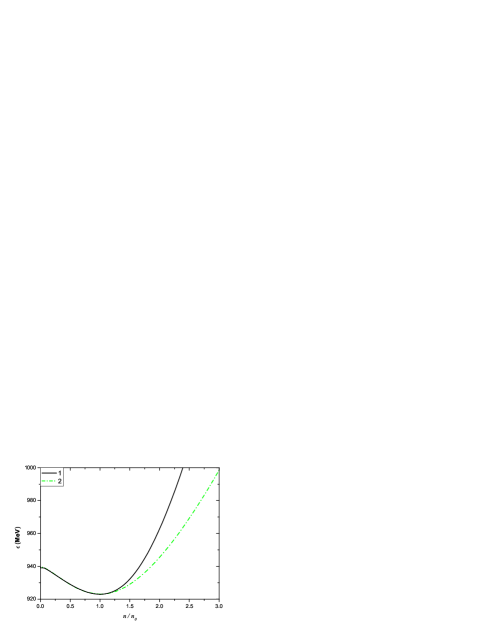
Figure 2: Equation of state for iso-symmetric uniform nuclear matter, given by RMFT (line 1) and by RHA or QRMFT (line 2)

The equations of state for RHA and QRMFT are the same. It means that the quantum correction on RHA given by the last term of (37) is practically zero, and therefore the RHA solution of the problem defined by the Lagrangian (1) is an excellent zeroth order approximation for the next order quantum correction.

On the other hand, Fig. 3

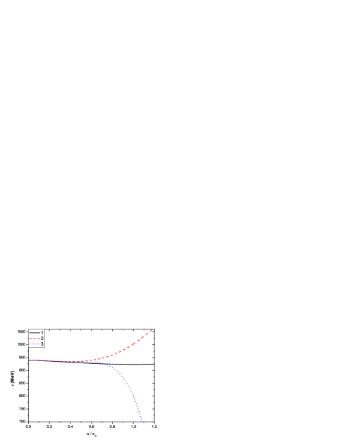
Figure 3: Line 1: The RMFT equation of state. Line 2: The equation of state obtained by adding the fourth term of (37) on line 1. Line 3: The equation of state obtained by adding the fifth term of (37) on line 2.

shows that the quantum corrections on RMFT given by the last two terms of (37) are quite big, and make the equation of state qualitatively distorted. The series of quantum corrections seems not converge. It means that the Walecka’s RMFT solution of the problem defined by the Lagrangian (1) is not a good zeroth order approximation for the next order quantum corrections.

Of course, these results are for the problem defined by the Lagrangian (1). The situation should be checked case by case. The smallness of the correction on RHA is due to the cancelation between $\tilde{n},B$ and $C$. In the problem considered above, the cancelation is almost complete. However, the completeness will not be always. There is evidence showing that if the Lagrangian (1) is generalized in a way with the term $\frac{1}{2}m_{\sigma}^{2}\Phi^{2}$ being substituted by

$$U(\Phi)=\frac{1}{2}m_{\sigma}^{2}\Phi^{2}\left(1+a_{1}\Phi+a_{2}\Phi^{2}\right),$$ (45)

the quantum corrections on RHA may be non-zero but still small, for non-zero $a_{1}$ and $a_{2}$.

V Conclusions and discussions

Shortly speaking, our conclusions are:

1. The RHA covers the leading part of quantum field theory for nuclear systems, but the simple RMFT does not.

2. The residual interaction $H^{\prime}$ in Eq. (36) may be considered by perturbation theory, with the expansion scheme used in traditional nuclear physics.

3. QRMFT, which we proposed here, is therefore an easy and practical way for handling nuclear problems until quark degrees of freedom become important.

In our formalism, the mean field $\phi$ is a free parameter. The equivalence (32) is true for its any value. This makes us have right to choose its value so that the solution of our problem becomes easy and accurate. RMFT, RHA and QRMFT chose it in different ways, and then obtained different accuracies and convergence properties for their solutions. Among them the QRMFT is the best. In this way we solve the problem of non-convergence, which the loop expansion procedure also encountered beforefps . Different value of $\phi$ means different vacuum in the nuclear matter. The theory with a change of vacuum must be non-perturbative. The vacuum $|0\rangle^{\prime}$ in nuclear matter satisfies the condition

$$a^{\prime}(k)|0\rangle^{\prime}=0.$$ (46)

By (28) we see

$$a(k)|0\rangle^{\prime}=\phi\sqrt{\frac{\omega_{\sigma}(2\pi)^{3}}{2}}\delta^{3}(\textbf{k})|0\rangle^{\prime}.$$ (47)

It means $|0\rangle^{\prime}$ is a coherent state of the original scalar mesons. Scalar mesons develop a Bose condensation in nuclear matter.

Beside the scalar meson, any kinds of mesons may develop Bose condensation in nuclear matter under suitable condition. The most often talked is the $\pi$-condensation. We have even proven that the $\pi$-condensation may develop in the Walecka modelz4 ; wyw . In non-uniform nuclear systems, for example the finite nuclei, the vector meson condensation may develop. In these cases, the quantum fluctuation of the condensed mesons should also be considered. The meson condensation is described by a classical meson field, and the quantum fluctuation is described by its quantum corrections. The method developed here may be useful for considering these corrections.

References

• (1) T. D. Lee and M. Margulies, Phys. Rev. D 11 (1975) 1591
• (2) J. D. Walecka, Annals of Physics 83 (1974) 491.
• (3) S. A. Chin, Annals of Physics 108 (1977) 301.
• (4) F. E. Serr and J. D. Walecka, Phys. Lett. 79B (1978) 10.
• (5) B.D. Serot and J.D. Walecka, in: J.W. Negele and E. Vogt, Eds, Advances in Nuclear Physics vol. 16, Plenum, New York (1986).
• (6) R. J. Furnstahl, R. J. Perry and B. D. Serot, Phys. Rev. C 40 (1989) 321
• (7) S. A. Chin, Physics Letters 62B (1976) 263.
• (8) J. Boguta and H. Stocker, Phys. Lett. 120B (1983) 289.
• (9) Qi-Ren Zhang, Phys. Ener. Fort. Phys. Nucl. 3 (1979) 75 (in Chinese)
• (10) M. Rufa, P.-G. Reinhard, J. A. Maruhn, W. Greiner, and M. R. Strayer, Phys. Rev. C 38 (1988) 390.
• (11) D. H. Rischke, M. I. Gorenstein, H. Stöcker and W. Greiner, Z. Phys. C 51 (1991) 485.
• (12) Bodmer AR, Nucl. Phys. A 526 (1991) 703.
• (13) Qi-Ren Zhang and Xun-Gui Li, J. Phys. G18 (1992) L111.
• (14) Chun-Yuan Gao and Qi-Ren Zhang, Int. J. Mod. Phys. E11 (2002) 55.
• (15) Qi-Ren Zhang, Commun. Theor. Phys. (Beijing, China) 47 (2007)1017.
• (16) I. Tamm, J. Phys. (U.S.S.R) 9 (1945) 449.
• (17) S. M. Dancoff, Phys. Rev. 78 (1950) 382.
• (18) W. D. Myers and W. J. Swiatecki, Annals of Physics 84 (1974) 186.
• (19) B. Friedman and V. R. Pandharipande, Phys. Lett. 100B (1981) 205.
• (20) Qi-Ren Zhang and Walter Greiner, Mod. Phys. Lett. A10 (1995) 2809.
• (21) Q.-R. Zhang, C.-Y. Gao, and Y.-W. Wu, in Nonequilibrium and Nonlinear Dynamics in Nuclear and other Finite System (ed. Z.-X. Li et.al. AIP Conference Proceedings 597, 2001) 118.