Sequential Compressed Sensing

Abstract

Compressed sensing allows perfect recovery of sparse signals (or signals sparse in some basis) using only a small number of random measurements. Existing results in compressed sensing literature have focused on characterizing the achievable performance by bounding the number of samples required for a given level of signal sparsity. However, using these bounds to minimize the number of samples requires a-priori knowledge of the sparsity of the unknown signal, or the decay structure for near-sparse signals. Furthermore, there are some popular recovery methods for which no such bounds are known.

In this paper, we investigate an alternative scenario where observations are available in sequence. For any recovery method, this means that there is now a sequence of candidate reconstructions. We propose a method to estimate the reconstruction error directly from the samples themselves, for every candidate in this sequence. This estimate is universal in the sense that it is based only on the measurement ensemble, and not on the recovery method or any assumed level of sparsity of the unknown signal. With these estimates, one can now stop observations as soon as there is reasonable certainty of either exact or sufficiently accurate reconstruction. They also provide a way to obtain “run-time” guarantees for recovery methods that otherwise lack a-priori performance bounds.

We investigate both continuous (e.g. Gaussian) and discrete (e.g. Bernoulli) random measurement ensembles, both for exactly sparse and general near-sparse signals, and with both noisy and noiseless measurements.

I Introduction

In compressed sensing (CS) [1, 2] a few random linear measurements of a signal are taken, and the signal is recovered using the additional knowledge that either the signal or some linear transform of it is sparse. These ideas have generated a lot of excitement in the signal processing and machine learning communities, and have been applied to a range of applications such as magnetic resonance imaging (MRI) [3], computational photography [4], wireless networks [5], and structure discovery in biological networks [6].

The applications where compressed sensing is most beneficial (e.g. MRI) have a high cost of acquiring each additional sample. If this cost (in terms of time, power, e.t.c) is high as compared to the cost of computation, then it is suitable to use sophisticated recovery algorithms which include the $\ell_{1}$-based basis pursuit [7], greedy approaches [8], and even non-convex ($\ell_{p}$) or iterative formulations [9, 10, 11] to enable recovery from fewer measurements.

While some of the recovery methods, especially those based on $\ell_{1}$-regularization, have analytically provable performance guarantees [12, 2], others, such as non-convex $\ell_{p}$, reweighted $\ell_{1}$ [11], and sparse Bayesian learning (SBL) [13] do not, and they have been shown empirically to often require even fewer samples than $\ell_{1}$-based methods. Furthermore, when guarantees do exist, they have been empirically observed to sometimes be highly pessimistic and may require large dimensions to hold with high probability [1, 14]. Another drawback is that much of the existing analysis characterizes how many measurements are needed for a signal with a given sparsity level. However, as the sparsity level is often not known a-priori, it can be very challenging to use these results in practical settings.

In this paper we take an alternative approach and we develop estimates and bounds for the reconstruction error using only the observations, without any a-priori assumptions on signal sparsity, or on the reconstruction method. We consider a scenario where one is able to get observations in sequence, and perform computations in between observations to decide whether enough samples have been obtained – thus allowing to recover the signal either exactly or to a given tolerance from the smallest possible number of random observations. This, however, requires a computationally efficient approach to detect exactly when enough samples have been received. To get an intuition behind our approach – suppose that we first attempt to reconstruct the signal while withholding some available observations, akin to cross-validation. The observations correspond to a known linear function of the true signal, so if the reconstructed signal is quite different from the true signal, then the same linear function applied to our recovered signal will result in a value that is far from the actual observation, with high probability. Our results provide estimates of the reconstruction error based on the statistics of the measurement model. They can thus be used to provide ’run-time’ guarantees even for decoders that are otherwise not amenable to analysis.

We first consider the case when noiseless measurements are taken using the random Gaussian (or generic continuous) ensemble, and we show that simply checking for one-step agreement provides a way to check exactly when enough samples have been received. Suppose that after receiving $M$ samples $y_{i}={\mathbf{a}}_{i}^{\prime}{\mathbf{x}},~{}i=1,..,M$, we apply a sparse reconstruction method of our choice, and obtain a solution $\hat{\mathbf{x}}^{M}$ satisfying all the $M$ measurements. We can use any sparse decoder, including greedy matching pursuit, SBL, $\ell_{p}$ formulations, and even the brute-force decoder, but we require that the solution at each step $M$ satisfies $y_{i}={\mathbf{a}}_{i}^{\prime}\hat{\mathbf{x}}^{M}$, for $i=1,..,M$. For example, in the case of basis pursuit, we would solve

$$\hat{\mathbf{x}}^{M}=\arg\min||{\mathbf{x}}||_{1}~{}~{}~{}\mbox{s.t.}~{}~{}~{}{\mathbf{a}}_{i}^{\prime}{\mathbf{x}}=y_{i},~{}~{}i=1,..,M.$$ (1)

Next, we receive one more measurement, and check for one step agreement: i.e. if $\hat{\mathbf{x}}^{M+1}=\hat{\mathbf{x}}^{M}$, then the decoder declares $\hat{\mathbf{x}}^{M}$ to be the reconstruction and stops requesting new measurements. In Section III we show in Propositions 1 and 2 that this decoder gives exact reconstruction with probability one.

For some other measurement ensembles, such as random Bernoulli and the ensemble of random rows from a Fourier basis, the one-step agreement stopping rule no longer has zero probability of error. We modify the rule to wait until $T$ subsequent solutions $\hat{\mathbf{x}}^{M}$, …, $\hat{\mathbf{x}}^{M+T}$ all agree. In Section IV we show in Proposition 3 that in the Bernoulli case the probability of making an error using this stopping rule decays exponentially with $T$, allowing trade-off of error probability and delay.

In Sections V and VI we show how the error in reconstruction can be estimated from the sequence of recovered solutions. We first present analysis for the Gaussian measurement ensemble in Proposition 4, and then generalize to any sensing matrices with i.i.d. entries. This enables the decoder to stop once the error is below a required tolerance – even for signals that are not exactly sparse, but in which the energy is largely concentrated in a few components, or for measurements which are corrupted by noise.

Finally, in Section VII we motivate the need for efficient solvers in the sequential setting. We consider the basis pursuit sparse solver and show that rather than re-solving the problem from scratch after an additional measurement is received, we could use an augmented linear program that uses the solution at step $M$ to guide its search for the new solution. We show empirically that this approach significantly reduces computational complexity.

During the review process we learned about a very recent analysis in [15] for the cross-validation setting, using the Johnson-Lindenstrauss lemma. We describe similarities and differences from our work in the discussion in Section V. Our current paper extends our earlier results presented in [16].

II Brief overview of compressed sensing

As there is no dearth of excellent tutorials on compressed sensing [17, 1, 2], in this section we give only a brief outline mainly to set the stage for the rest of the paper. At the heart of compressed sensing lies the sparse recovery problem, which tries to reconstruct an unknown sparse signal ${\mathbf{x}}$ from a limited number of measurements ${\mathbf{y}}=A{\mathbf{x}}$, where $A\in\mathbb{R}^{M\times N}$, $M<<N$. Much of excitement in the field stems from the fact that the hard combinatorial problem of searching for sparse solutions in the affine space $\{{\mathbf{x}}:{\mathbf{y}}=A{\mathbf{x}}\}$ under certain suitable conditions can be solved exactly via various tractable methods. The most widely known methods include greedy matching pursuit and its variants [8], and approaches based on convex optimization, using $\ell_{1}$ norms as a proxy for sparsity [7]:

$$\min\|{\mathbf{x}}\|_{1}~{}~{}~{}\mbox{ subject to }~{}~{}{\mathbf{y}}=A{\mathbf{x}}.$$ (2)

An early sufficient condition for sparse recovery [18] states that the formulation in (2) recovers the unique sparse solution if $A$ is well-posed and ${\mathbf{x}}$ is sparse enough, i.e. if $\|{\mathbf{x}}\|_{0}<\frac{1+1/M(A)}{2}$, where $M(A)=\max_{i\neq j}|{\mathbf{a}}_{i}^{\prime}{\mathbf{a}}_{j}|$, and $A$ has columns ${\mathbf{a}}_{i}$ normalized to $1$. However, this simple condition is very pessimistic. Much tighter conditions are obtained by considering larger subsets of columns of $A$, e.g. the restricted isometry property (RIP) depends on the maximum and minimum singular values over all $M\times K$ submatrices of $A$ [12]. Namely, a matrix $A$ satisfies the $K$-RIP with constant $\delta_{K}$ if $(1-\delta_{K})\|{\mathbf{x}}\|_{2}^{2}\leq\|A{\mathbf{x}}\|_{2}^{2}\leq(1+\delta_{K})\|{\mathbf{x}}\|_{2}^{2}$ for every ${\mathbf{x}}$ which has at most $K$ non-zero entries. While enabling much tighter sufficient conditions for recovery of sparse signals [12], the RIP is very costly (exponential in $K$) to check for a given matrix.

Results in compressed sensing take advantage of RIP by bringing in the theory of random matrices into the picture. In compressed sensing we receive random measurements ${\mathbf{y}}=\Psi{\mathbf{s}}$ where the unknown signal of interest ${\mathbf{s}}$ is itself sparse in some basis, i.e. ${\mathbf{s}}=\Phi{\mathbf{x}}$, with ${\mathbf{x}}$ sparse. Hence the problem reduces to finding sparse solutions satisfying ${\mathbf{y}}=\Psi\Phi{\mathbf{x}}=A{\mathbf{x}}$, where $A=\Psi\Phi$ is a random matrix.

A collection of results have been established that RIP holds for random matrices of certain size from given ensembles: Gaussian, Bernoulli, random Fourier rows [12, 2, 14]. The general conclusion of these results is that the convex $\ell_{1}$ formulation can recover (with high probability) a signal ${\mathbf{x}}\in\mathbb{R}^{N}$ with $K$ non-zeros from only $CK\log(N)$ measurements, where $C$ is a constant depending on the random measurement ensemble. This is indeed remarkable – as it only requires a logarithmic dependence of the number of measurements on $N$.

Figure 1: Histogram of the stopping times distribution for Gaussian and Bernoulli measurement ensembles: $N=100$, and $K=10$, and $\ell_{1}$ decoding.

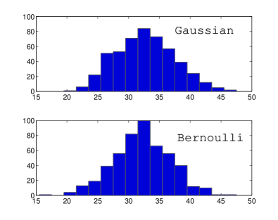
However, when each additional measurement is very costly there are several problems with these bounds – firstly, since they are high-probability results independent of ${\mathbf{y}}$, they tend to be conservative, and also the constants $C$ are typically generous upper-bounds. Secondly, the number of measurements depends on the number of non-zero components of ${\mathbf{x}}$ which may not be known a-priori. Finally, there are successful approaches which we mentioned in Section I for which no such results are available.

In Figure 1 we illustrate the drawbacks of using upper bounds on the number of measurements. We find the minimum number $M$ of random samples which were needed to recover a sparse signal ${\mathbf{x}}$ with $N=100$, and $K=10$ from random Gaussian and Bernoulli measurements using the $\ell_{1}$-formulation in (2), over $500$ random trials. We plot a histogram of these numbers, and we see that they exhibit high variance, and so relying on conditions that guarantee recovery with high probability often means taking many unnecessary samples. This motivates the need for sequential compressed sensing scenario that can adaptively minimize the number of samples for each observed ${\mathbf{y}}$, which we describe next.

III Stopping rule in the noiseless continuous case

We now analyze the sequential CS approach for the case when the measurements vectors ${\mathbf{a}}_{i}$ come from a continuous ensemble (e.g., the i.i.d. Gaussian ensemble), having the property that with probability $1$ a new vector ${\mathbf{a}}_{M+1}$ will not be in any lower-dimensional subspace determined by previous vectors $\{{\mathbf{a}}_{i}\}_{i=1}^{M}$. Suppose that the underlying sparse signal ${\mathbf{x}}^{*}\in\mathbb{R}^{N}$ has $K$ non-zero components (we denote the number of non-zero entries in ${\mathbf{x}}$ by $\|{\mathbf{x}}\|_{0}$). We sequentially receive random measurements $y_{i}={\mathbf{a}}_{i}^{\prime}{\mathbf{x}}^{*}$, where for concreteness ${\mathbf{a}}_{i}\sim\mathcal{N}(0,I)$ is a $N$-vector of i.i.d. Gaussian samples, but the analysis also holds if entries of ${\mathbf{a}}_{i}$ are i.i.d. samples of an arbitrary continuous random variable. At step $M$ we use a sparse solver of our choice to obtain a feasible solution $\hat{\mathbf{x}}^{M}$ using all the received data. Results in compressed sensing [1, 14] indicate that if we use basis pursuit or matching pursuit methods, then after receiving around $M\propto K\log(N)$ measurements we can recover the signal ${\mathbf{x}}^{*}$ with high probability. This requires the knowledge of $K$, which may not be available, and only rough bounds on the scaling constants are known. Our approach is different – we compare the solutions at step $M$ and $M+1$, and if they agree, we declare correct recovery.

Figure 2: A new constraint is added: ${\mathbf{a}}_{M+1}^{\prime}{\mathbf{x}}=y_{M+1}$. Probability that this hyperplane passing through ${\mathbf{x}}^{*}$ also passes through $\hat{\mathbf{x}}^{M}$ is zero.

Proposition 1

If in the Gaussian (generic continuous) measurement ensemble it holds that $\hat{\mathbf{x}}^{M+1}=\hat{\mathbf{x}}^{M}$, then $\hat{\mathbf{x}}^{M}={\mathbf{x}}^{*}$, with probability $1$.

Proof. Let ${\mathbf{y}}_{1:M}\triangleq[y_{1},...,y_{M}]^{\prime}$, and $A^{M}\triangleq[{\mathbf{a}}_{1},...,{\mathbf{a}}_{M}]^{\prime}$. Suppose that $\hat{\mathbf{x}}^{M}\neq{\mathbf{x}}^{*}$. We have that ${\mathbf{y}}_{1:M}=A^{M}\hat{\mathbf{x}}^{M}$ and ${\mathbf{y}}_{1:M}=A^{M}{\mathbf{x}}^{*}$: both ${\mathbf{x}}^{*}$ and $\hat{\mathbf{x}}^{M}$ belong to the $(N-M)$-dimensional affine space $\{{\mathbf{x}}~{}|~{}{\mathbf{y}}_{1:M}=A^{M}{\mathbf{x}}\}$. The next measurement passes a random hyperplane $y_{M+1}={\mathbf{a}}_{M+1}^{\prime}{\mathbf{x}}^{*}$ through ${\mathbf{x}}^{*}$ and reduces the dimension of the affine subspace of feasible solutions by $1$. In order for $\hat{\mathbf{x}}^{M}$ to remain feasible at step $M+1$, it must hold that ${\mathbf{y}}_{M+1}={\mathbf{a}}_{M+1}^{\prime}\hat{\mathbf{x}}^{M}$. Since we also have ${\mathbf{y}}_{M+1}={\mathbf{a}}_{M+1}^{\prime}{\mathbf{x}}^{*}$, then $\hat{\mathbf{x}}^{M}$ remains feasible only if $(\hat{\mathbf{x}}^{M}-{\mathbf{x}}^{*})^{\prime}{\mathbf{a}}_{M+1}=0$, i.e. if ${\mathbf{a}}_{M+1}$ falls in the $N-1$ dimensional subspace of $\mathbb{R}^{N}$ corresponding to $Null((\hat{\mathbf{x}}^{M}-{\mathbf{x}}^{*})^{\prime})$. As ${\mathbf{a}}_{M+1}$ is random and independent of $\hat{\mathbf{x}}^{M}$ and of the previous samples ${\mathbf{a}}_{1}$, …, ${\mathbf{a}}_{M}$, the probability that this happens is $0$ (event with measure zero). See Figure 2 for illustration. $\square$

Note that the proof implies that we can simplify the decoder to checking whether ${\mathbf{a}}_{M+1}^{\prime}\hat{\mathbf{x}}^{M}=y_{M+1}$, avoiding the need to solve for $\hat{\mathbf{x}}^{M+1}$ at the last step. Moreover, if using any sparse solver in the continuous ensemble case the solution $\hat{\mathbf{x}}^{M}$ has fewer than $M$ non-zero entries, then $\hat{\mathbf{x}}^{M}={\mathbf{x}}^{*}$ with probability 1.

Proposition 2

For a Gaussian (continuous) measurement ensemble, if $\|\hat{\mathbf{x}}^{M}\|_{0}<M$, then $\hat{\mathbf{x}}^{M}={\mathbf{x}}^{*}$ with probability $1$.

Proof. Denote the support of our unknown sparse vector ${\mathbf{x}}^{*}$ by $\mathcal{I}$, i.e. $\mathcal{I}=\{i~{}|~{}x^{*}_{i}\neq 0\}$. We next generate a random measurement matrix $A^{M}$. Let $A=A^{M}$ to simplify notation. We receive the corresponding measurements ${\mathbf{y}}=A{\mathbf{x}}^{*}$. Now $A$ is $M\times N$, with $M<N$. The key fact about random matrices with i.i.d. entries from a continuous distribution is that any $M\times M$ submatrix of $A$ is non-singular with probability $1$. We now argue that with probability 1 after receiving ${\mathbf{y}}$ there will not exist another sparse feasible solution $\hat{\mathbf{x}}\neq{\mathbf{x}}^{*}$, i.e. $\hat{\mathbf{x}}$ with fewer than $M$ non-zero entries satisfying ${\mathbf{y}}=A\hat{\mathbf{x}}$ . We consider all possible sparse supports $\mathcal{J}\subset\{1,..,N\}$, with $|\mathcal{J}|<M$, and show that a feasible solution $\hat{\mathbf{x}}\neq{\mathbf{x}}^{*}$ can have this support only with probability 0. There are two cases: $\mathcal{I}\subset\mathcal{J}$ and $\mathcal{I}\neq\mathcal{I}\cap\mathcal{J}$.

Figure 3: Gaussian ensemble example: $N=100$, and $K=10$. (Top): $~{}\|\hat{\mathbf{x}}^{M}\|_{0}$. (Middle): $~{}\|\hat{\mathbf{x}}^{M}\|_{1}$. (Bottom): $~{}\|{\mathbf{x}}^{*}-\hat{\mathbf{x}}^{M}\|_{2}$.

First suppose $\mathcal{I}\subset\mathcal{J}$, $|\mathcal{J}|<M$, and suppose there exists some feasible $\hat{\mathbf{x}}$ supported on $\mathcal{J}$. Then $\hat{\mathbf{x}}-{\mathbf{x}}^{*}\in Null(A)$, and support of $\hat{\mathbf{x}}-{\mathbf{x}}^{*}$ is a subset of $\mathcal{J}$, hence it is smaller than $M$. But that means that there is a subset of fewer than $M$ columns of $A$ that are linearly dependent, which can only happen with probability zero.

Now consider the case $\mathcal{I}\neq\mathcal{I}\cap\mathcal{J}$. For a fixed $\mathcal{I}$ we consider all such possible sets $\mathcal{J}$, with $|\mathcal{J}|<M$. First fix one such set $\mathcal{J}$. We use the notation $\mathcal{I}\backslash\mathcal{J}=\{~{}i\in I~{}|~{}i\notin J\}$. Note that we have ${\mathbf{y}}=A{\mathbf{x}}^{*}=A_{\mathcal{J}}{\mathbf{x}}^{*}_{\mathcal{J}}+A_{\mathcal{I}\backslash\mathcal{J}}{\mathbf{x}}^{*}_{\mathcal{I}\backslash\mathcal{J}}$. Let $\tilde{{\mathbf{y}}}=A_{\mathcal{I}\backslash\mathcal{J}}{\mathbf{x}}^{*}_{\mathcal{I}\backslash\mathcal{J}}$. Now since we require $\hat{\mathbf{x}}$ to be feasible, we also need ${\mathbf{y}}=A\hat{\mathbf{x}}=A_{\mathcal{J}}\hat{\mathbf{x}}_{\mathcal{J}}$ which would imply that $\tilde{{\mathbf{y}}}=A_{\mathcal{J}}(\hat{\mathbf{x}}_{\mathcal{J}}-{\mathbf{x}}^{*}_{\mathcal{J}})$. This means that the vector $\tilde{{\mathbf{y}}}$ would also have to be in the span of $A_{\mathcal{J}}$. However, $\tilde{{\mathbf{y}}}$ is a random vector in $\mathbb{R}^{M}$ (determined by ${\mathbf{x}}^{*}$ and $A_{\mathcal{I}\backslash\mathcal{J}}$), and span of $A_{\mathcal{J}}$ is an independent random subspace of dimension strictly less than $M$. Hence, the event that $\tilde{{\mathbf{y}}}$ also falls in the span of $A_{\mathcal{J}}$ has measure zero. This means that for a fixed $\mathcal{J}$ a distinct sparse solution can only exist with probability $0$. Now the number of possible subsets $\mathcal{J}$ is finite (albeit large), so even when we take all such supports $\mathcal{J}$, a distinct sparse solution supported on $\mathcal{J}$ can only exist with probability $0$. Hence, with probability $1$ there is only one solution with $\|{\mathbf{x}}\|_{0}<M$, namely ${\mathbf{x}}^{*}$. $\square$

This proposition allows to stop making measurements when a feasible solution has less than $M$ nonzero entries – avoiding the need to make the last $(M+1)$-st measurement.

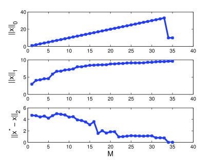
Consider an example in Figure 3 with $N=100$, and $K=10$. We keep receiving additional measurements and solving (1) until we reach one-step agreement, $\hat{\mathbf{x}}^{M}=\hat{\mathbf{x}}^{M+1}$. The top plot shows that $\|\hat{\mathbf{x}}^{M}\|_{0}$ increases linearly with $M$ until one step agreement occurs at $M=35$, at which point it drops to $K=10$ and a and we recover the correct sparse solution, $\hat{\mathbf{x}}^{M}={\mathbf{x}}^{*}$. The middle plot shows the monotonic increase in $\|\hat{\mathbf{x}}^{M}\|_{1}$ (as the feasible set is shrinking with $M$). The bottom plot shows the error-norm of the solution, $\|\hat{\mathbf{x}}^{M}-{\mathbf{x}}^{*}\|_{2}$. On average it tends to go down with more observations, but non-monotonically. After $M=35$ the error becomes zero. We see that in the ideal conditions of no measurement noise, sparse unknown signals and Gaussian measurement ensembles, the number of measurements can be indeed minimized by a simple stopping rule.

IV Stopping rule in the Bernoulli case

In this section we study a simple but popular measurement ensemble that is not one of the generic continuous ensembles described in the previous section. Suppose that the measurement vectors ${\mathbf{a}}_{i}$ have equiprobable i.i.d. Bernoulli entries $\pm 1$. A difference emerges from the Gaussian case: the probability that all $M\times M$ submatrices of $A^{M}$ are non-singular is no longer $0$. This makes it possible (with non-zero probability) for $\hat{\mathbf{x}}^{M+1}$ to agree with $\hat{\mathbf{x}}^{M}$ even though $\hat{\mathbf{x}}^{M}\neq{\mathbf{x}}^{*}$, and for erroneous solutions $\hat{\mathbf{x}}^{M}$ to have cardinality less than $M$. We modify the stopping rule to require agreement for several steps - success is declared only when last $T$ solutions all agree. We show in proposition 3 that the probability of error decays exponentially with $T$. We use the following Lemma from [19]:

Lemma 1 (Tao and Vu)

Let ${\mathbf{a}}$ be an i.i.d. equiprobable Bernoulli vector with ${\mathbf{a}}\in\{-1,1\}^{N}$. Let $W$ be a deterministic $d$-dimensional subspace of $\mathbb{R}^{N}$, $0\leq d<N$. Then $P({\mathbf{a}}\in W)\leq 2^{d-N}$.

We are now ready to establish the following claim:

Proposition 3

Consider the Bernoulli measurement case. If $\hat{\mathbf{x}}^{M}=\hat{\mathbf{x}}^{M+1}=...=\hat{\mathbf{x}}^{M+T}$, then $\hat{\mathbf{x}}^{M}={\mathbf{x}}^{*}$ with probability greater than or equal to $1-2^{-T}$.

Proof. Suppose that $\hat{\mathbf{x}}^{M}\neq{\mathbf{x}}^{*}$. Denote the support of ${\mathbf{x}}^{*}$ by $\mathcal{I}$ and the support of $\hat{\mathbf{x}}^{M}$ by $\mathcal{J}$. At step $M$ we have $A^{M}{\mathbf{x}}^{*}=A^{M}\hat{\mathbf{x}}^{M}$. Let $W=\{{\mathbf{a}}~{}|~{}(\hat{\mathbf{x}}^{M}-{\mathbf{x}}^{*})^{\prime}{\mathbf{a}}=0\}$, i.e. the nullspace of $(\hat{\mathbf{x}}^{M}-{\mathbf{x}}^{*})^{\prime}$. Then $W$ is an $(N-1)$-dimensional subspace of $\mathbb{R}^{N}$.

Given a new random Bernoulli sample ${\mathbf{a}}_{M+1}$, the vector $\hat{\mathbf{x}}^{M}$ can remain feasible at step $M+1$ only if $(\hat{\mathbf{x}}^{M}-{\mathbf{x}}^{*})^{\prime}~{}{\mathbf{a}}_{M+1}=0$, i.e. if ${\mathbf{a}}_{M+1}$ falls into $W$. By Lemma 1, the probability that ${\mathbf{a}}_{M+1}\in W$ is a most $1/2$. The same argument applies to all subsequent samples of ${\mathbf{a}}_{M+i}$ for $i=1,..,T$, so the probability of having $T$-step agreement with an incorrect solution is bounded above by $2^{-T}$. $\square$

Note that as in the discussion for the continuous case, we can simply check that ${\mathbf{a}}_{M+i}^{\prime}\hat{\mathbf{x}}^{M}=y_{M+i}$ for $i=1,...,T$, avoiding the need to solve for $\hat{\mathbf{x}}^{M+T}$.

We now pursue an alternative heuristic analysis, more akin to Proposition 2. For the Bernoulli case, $\|\hat{\mathbf{x}}^{M}\|_{0}<M$ does not imply $\hat{\mathbf{x}}^{M}={\mathbf{x}}^{*}$. However, we believe that once we obtain enough samples so that $N^{2}2^{1-M}$ $\ll 1$ then $\|\hat{\mathbf{x}}^{M}\|_{0}<M$ will imply that $\hat{\mathbf{x}}^{M}={\mathbf{x}}^{*}$ with high probability. Since the elements of ${\mathbf{a}}_{i}$ belong to finite set $\{-1,1\}$, an $M\times M$ submatrix of $A^{M}$ can be singular with non-zero probability. Surprisingly, characterizing this probability is a very hard question. It is conjectured [19] that the dominant source of singularity is the event that two columns or two rows are equal or opposite in sign. This leads to the following estimate (here $X_{M}$ is $M\times M$):

$$P(\det X_{M}=0)=(1+o(1))M^{2}2^{1-M}.$$ (3)

However the very recent best provable bound on this probability is still rather far: $P(\det X_{M}=0)=((\frac{3}{4}+o(1))^{M})$ [19]. If we assume that the simple estimate based on pairs of columns is accurate, similar analysis shows that the probability that a random $\pm 1$ $M\times N$ matrix with $M\ll N$ having all $M\times M$ submatrices non-singular is $(1+o(1))N^{2}2^{1-M}$.

V Near-sparse signals

In practical settings, e.g. when taking Fourier and wavelet transforms of smooth signals, we may only have approximate sparseness: a few values are large, and most are very small. In this section we extend our approach to this case; again, and in contrast to existing work, we do not need to assume a specific near-sparse structure, like power-law decay, but instead provide bounds that hold for any signal.

Figure 4: Geometry of the analysis for near-sparse signals. The unknown reconstruction error is related to $d(\hat{\mathbf{x}}^{M},H_{M+T})$ and the angle $\theta$ between the line from ${\mathbf{x}}^{*}$ to $\hat{\mathbf{x}}^{M}$ and the affine space $H_{M+T}$ defined by the new measurements.

The exact one-step agreement stopping rule from Section III is vacuous for near-sparse signals, as $\|{\mathbf{x}}^{*}\|_{0}=N$, and all samples are needed for perfect recovery. We start by considering Gaussian measurements, and show that we can gather information about the current reconstruction error by obtaining a small number of additional measurements, and computing the distance between the current reconstruction and the affine space determined by these new measurements. The reconstruction error is then equal to an unknown constant times this distance:

$$\|{\mathbf{x}}^{*}-\hat{\mathbf{x}}^{M}\|_{2}=C_{T}~{}d(\hat{\mathbf{x}}^{M},H_{M+T}),$$ (4)

where $H_{M+T}\triangleq\{x~{}|~{}y_{i}={\mathbf{a}}_{i}^{\prime}x,~{}1\leq i\leq M+T\}$ is the affine space determined by all $M+T$ measurements, $C_{T}$ is a random variable that we will bound, and $d(\hat{\mathbf{x}}^{M},H_{M+T})$ denotes the distance from $\hat{\mathbf{x}}^{M}$ to $H_{M+T}$. We characterize $E[C_{T}]$ and $Var[C_{T}]$ – this gives us a confidence interval on the reconstruction error using the observed distance $d(\hat{\mathbf{x}}^{M},H_{M+T})$. We can now stop taking new measurements once the error falls below a desired tolerance. Note that our analysis does not assume a model of decay, and bounds the reconstruction error by obtaining a small number of additional measurements, and computing the prediction error. In contrast, some related results in CS literature assume a power-law decay of entries of ${\mathbf{x}}^{*}$ (upon sorting) and show that with roughly $O(K\log N)$ samples, $\hat{\mathbf{x}}^{M}$ in (1) will have similar error to that of keeping the $K$ largest entries in ${\mathbf{x}}^{*}$ [1].

We now outline the analysis leading to a bound based on (4). Consider Figure 4. Let $H_{M}=\{{\mathbf{x}}:A^{M}{\mathbf{x}}={\mathbf{y}}_{1:M}\}$ be the subspace of feasible solutions after $M$ measurements. Both ${\mathbf{x}}^{*}$ and $\hat{\mathbf{x}}^{M}$ lie in $H_{M}$. The affine space $H_{M+T}$ is contained in $H_{M}$. Let $L=N-M$, and $\theta_{T}$ be the angle between the vector $\hat{\mathbf{x}}^{M}-{\mathbf{x}}^{*}$ and the affine space $H_{M+T}$. Both are contained in the $L$-dimensional space $H_{M}$. Centering around ${\mathbf{x}}^{*}$, we see that $\theta_{T}$ is the angle between a fixed vector in $R^{L}$ and a random $L-T$ dimensional subspace of $R^{L}$, and the constant $C_{T}$ in (4) is equal to $\frac{1}{\sin(\theta_{T})}$:

$$\|{\mathbf{x}}^{*}-\hat{\mathbf{x}}^{M}\|_{2}=\frac{d(\hat{\mathbf{x}}^{M},H_{M+T})}{\sin(\theta_{T})},$$ (5)

We next analyze the distribution of $\theta_{T}$ and hence of $C_{T}$. In distribution, $\theta_{T}$ is equivalent to the angle between a fixed $L-T$ dimensional subspace, say the one spanned by the last $L-T$ coordinates, and an i.i.d. Gaussian vector (whose direction falls uniformly on a unit sphere in $\mathbb{R}^{L}$). This holds because the distribution of an i.i.d. Gaussian sample does not get changed after applying an arbitrary orthogonal transformation. Let $H$ be the span of the last $L-T$ coordinate vectors, and ${\mathbf{h}}$ be i.i.d. Gaussian. Then:

$$C_{T}=\frac{1}{\sin(\theta)}=\sqrt{\sum_{i=1}^{L}h_{i}^{2}}~{}\mbox{\Large/}~{}\sqrt{\sum_{i=1}^{T}h_{i}^{2}}.$$ (6)

Using the properties of $\chi_{L}$, $\chi^{2}_{L}$, and inverse-$\chi^{2}_{L}$ distributions [20] and Jensen’s inequality, we have an estimate of the mean $E[C_{T}]\approx\sqrt{\frac{L}{T}}$ and an upper bound on both the mean and the variance:

$$E\left[C_{T}\right]\leq\sqrt{\frac{L-2}{T-2}},$$ (7)

$$Var\left[C_{T}\right]\leq\frac{L-2}{T-2}-\frac{L}{T}.$$ (8)

We describe the analysis in Appendix A. Using these bounds in conjunction with the Chebyshev inequality, $p(|a-E[a]|\geq k\sigma_{a})\leq\frac{1}{k^{2}}$, we have the following result:

Figure 5: (Top) sample mean, estimate of the mean, and a bound on the mean of $C_{T}$. (Bottom) sample standard deviation, and a bound on the standard deviation of $C_{T}$. Sample mean is based on 1000 samples. $L=100$.

Proposition 4

In the Gaussian measurement ensemble we have: $\|{\mathbf{x}}^{*}-\hat{\mathbf{x}}^{M}\|_{2}\leq\bar{C}^{k}_{T}~{}d(\hat{\mathbf{x}}^{M},H_{M+T})$ with probability at least $1-\frac{1}{k^{2}}$, where $\bar{C}^{k}_{T}=\sqrt{\frac{L-2}{T-2}}+k\sqrt{\frac{L-2}{T-2}-\frac{L}{T}}$, for any $k>0$.

Figure 6: (Top) Error confidence bounds and actual errors for a sparse signal, $N=100$, $T=5$, $K=10$. (Bottom): Error confidence bound and actual errors for a signal with power-law decay, $N=1000$, $T=10$.

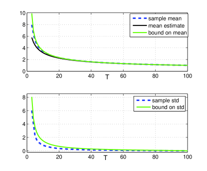
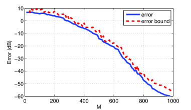
In Figure 5 (top) we plot the mean estimate, and our bound in (7) for $C_{T}$ and (bottom) the standard deviation bound for $L=100$ and a range of $T$. We compare them to sample mean and standard deviation of $C_{T}$ based on $5000$ samples. The figure shows that both bounds provide very good approximation for most of the range of $T>2$, and also that the standard deviation quickly falls off with $T$, giving tight confidence intervals. In Figure 6 we perform numerical experiments with two example signals, a sparse signal, $N=100$, $K=10$, $T=5$ (top) and a near-sparse signal with power-law decay, $N=1000$, $T=10$ (bottom). We use basis pursuit to recover the signals as we obtain progressively more measurements, and we compare our error bounds (via Chebyshev inequality) to the actual errors. We see that the bounds reliably indicate the reconstruction error – after a small delay of $T$ additional measurements. We have used basis pursuit in the experiments, but we could substitute any sparse solver instead, for example we could have also computed error estimates for matching pursuit.

V-A Analysis for More General Ensembles

To get the bound in (4) we characterized the distribution of $\frac{1}{\sin(\theta_{T})}$ and used the properties of the Gaussian measurement ensemble. Analysis of $\theta_{T}$ for general ensembles is challenging. We now consider a simpler analysis which provides useful estimates when $T<<L$, i.e. the case of main interest for compressed sensing, and when the measurement coefficients $a_{ij}$ are from an i.i.d. zero-mean ensemble. The previous bound for the Gaussian case depended on both $M$, the number of samples used for the current reconstruction, and $T$, the number of extra samples. Now, in the following we give estimates and bounds that depend only on $T$, and in that sense could be weaker for the Gaussian case when $M$ is large; they are however more generally applicable – in particular we no longer require $\hat{\mathbf{x}}^{M}$ to satisfy the measurements exactly.

Suppose we have a current reconstruction $\hat{\mathbf{x}}$, and suppose ${\mathbf{x}}^{*}$ is the (unknown) true signal. We now take $T$ new samples $y_{i}={\mathbf{a}}_{i}^{\prime}{\mathbf{x}}^{*}$, for $1\leq i\leq T$. For each of these samples we compute $\hat{y}_{i}={\mathbf{a}}_{i}^{\prime}\hat{\mathbf{x}}^{M}$ to be the same vector ${\mathbf{a}}_{i}$ applied to the current reconstruction. Denote the current error vector by ${\boldsymbol{\delta}}=\hat{\mathbf{x}}^{M}-{\mathbf{x}}^{*}$, and compute $z_{i}=\hat{y}_{i}-y_{i}$, the deviations from the actual measurements. Then

$$z_{i}={\mathbf{a}}_{i}^{\prime}{\boldsymbol{\delta}},~{}~{}~{}1\leq i\leq T$$ (9)

The new measurements ${\mathbf{a}}_{i}$ are independent of $\hat{\mathbf{x}}$ and of ${\mathbf{x}}^{*}$, hence of ${\boldsymbol{\delta}}$. The $z_{i}$’s are i.i.d. from some (unknown) distribution, which has zero mean and variance $\|{\boldsymbol{\delta}}\|_{2}^{2}~{}Var(a_{ij})$. We can estimate $\|{\boldsymbol{\delta}}\|_{2}^{2}$ by estimating the variance of the $z_{i}$’s from the $T$ samples. The quality of the estimate will depend on the exact distribution of ${\mathbf{a}}_{ij}$.

Consider the case where ${\mathbf{a}}_{i}$ are i.i.d. Gaussian. Then $z_{i}$ is Gaussian as well. For simplicity suppose that $Var(a_{ij})=1$, then the distribution of $z_{i}$ is i.i.d. Gaussian with zero-mean and variance $\|{\boldsymbol{\delta}}\|_{2}^{2}$. Let $Z_{T}=\sum_{i=M+1}^{M+T}z_{i}^{2}$. Then $\tilde{Z}_{T}\triangleq\frac{Z_{T}}{\|\delta\|^{2}}\sim\chi^{2}_{T}$, i.e. $\chi^{2}$ random variable with $T$ degrees of freedom. Now to obtain a confidence interval for $\|{\boldsymbol{\delta}}\|_{2}^{2}$ we use the cumulative $\chi^{2}_{T}$ distribution. We pick a confidence level $1-\alpha$ (for some small $\alpha>0$), and we use the $\chi^{2}_{T}$ cumulative distribution to find the largest $z^{*}$ such that $p(\tilde{Z}_{T}\leq z^{*})\leq\alpha$.

During the review process a related analysis in [15] was brought to our attention: the paper considers compressed sensing in a cross-validation scenario, and it proposes to estimate the errors in the reconstruction from a few additional (cross-validation) measurements. The paper cleverly uses the Johnson-Lindenstrauss (JL) lemma to find out how many random measurements are needed for predicting the error to a desired accuracy. For Gaussian measurements ensembles our $\chi^{2}$-based analysis can be seen as a special case (where all the constants are computed explicitly since we use the exact sampling distribution of $Z_{T}$), but JL lemma also generalizes to other ensembles satisfying certain requirements on the decay of the tails [15, 21].

Figure 7: Comparison of $\chi^{2}$ and $\sin(\theta)$ analysis. Given a unit-norm vector ${\boldsymbol{\delta}}$, we obtain $T$ additional measurements, and compute our two estimates of $\|{\boldsymbol{\delta}}\|$. We plot the histogram of the estimates over 5000 trials with $N=250$, $T=25$, and (a) $M=0$, (b) $M=200$.

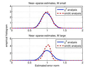
To compare our analysis in (5), based on $C_{T}$, to the one in (9) we note that the latter simply estimates the error $\|{\boldsymbol{\delta}}\|$ as $\|\frac{1}{\sqrt{T}}\tilde{A}{\boldsymbol{\delta}}\|$, where $\tilde{A}$ are the new measurements. Now unlike the analysis in (9), in (5) we require that the solution at step $M$ is feasible (matches all the measurements) and instead we compute the error of projecting ${\boldsymbol{\delta}}$ onto the null-space of $A$ and adjust it by the expected value of $\frac{1}{\sin(\theta)}$, i.e. we estimate $\|{\boldsymbol{\delta}}\|$ as $\sqrt{\frac{L}{T}}\|A^{\prime}(AA^{\prime})^{-1}A{\boldsymbol{\delta}}\|$, where $A$ includes all $M+T$ measurements. To compare the quality of the two estimates we conducted a simulation with $N=250$ and $T=25$, and computed the estimates for random unit-norm vectors ${\boldsymbol{\delta}}$. We plot the histograms for $M=0$ and $M=200$ over $5000$ trials in Figure 7. In the first case with $M=0$, we see that both estimates have about the same accuracy (similar error distributions), however as $M$ becomes appreciable the approach in (5) becomes more accurate.

VI Noisy case

Next we consider the sequential version of the noisy measurement setting, where the observations are corrupted by additive uncorrelated i.i.d. Gaussian noise with variance $\sigma_{n}^{2}$:

$$y_{i}={\mathbf{a}}_{i}^{\prime}{\mathbf{x}}+n_{i},~{}~{}~{}~{}i\in\{1,..,M\}.$$ (10)

To solve this problem one can adapt a variety of sparse solvers which allow inexact solutions $\hat{\mathbf{x}}^{M}$ in the sequential setting – for example matching pursuit methods with a fixed number of steps, or the noisy versions of basis pursuit. All of these methods have a trade-off between sparsity of the desired solution and the accuracy in representing the measurements. In the case of basis pursuit denoising a regularization parameter $\lambda$ balances these two costs:

$$\hat{\mathbf{x}}^{M}=\arg\min\frac{1}{2}\|{\mathbf{y}}_{1:M}-A^{M}{\mathbf{x}}\|_{2}^{2}+\lambda_{M}\|{\mathbf{x}}\|_{1}.$$ (11)

For greedy sparse solvers such as matching pursuit and its variants the trade-off is controlled directly by deciding how many columns of $A$ to use to represent ${\mathbf{y}}$. We are interested in a stopping rule which tells us that $\hat{\mathbf{x}}$ is reasonably close to ${\mathbf{x}}^{*}$ for any sparse solver and for any user defined choice of the trade-off between sparsity and measurement likelihood. We do not discuss the question of selecting a choice for the trade-off – we refer the readers to [22, 23] and also to [15] for a discussion of how this can be done in a cross-validation setting. Now, due to the presence of noise, exact agreement will not occur no matter how many samples are taken. We consider a stopping rule similar to the one in Section V. In principle, the analysis in (4) can be extended to the noisy case, but we instead follow the simplified analysis in Section V-A.

We establish that the reconstruction error can be bounded with high probability by obtaining a small number of additional samples, and seeing how far the measurements deviate from $\hat{y}_{i}={\mathbf{a}}_{i}^{\prime}\hat{\mathbf{x}}^{M}$. With such a bound one can stop receiving additional measurements once the change in the solution reaches levels that can be explained due to noise. The deviations $z_{i}$ now include contribution due to noise:

$$z_{i}=\hat{y}_{i}-y_{i}={\mathbf{a}}_{i}^{\prime}(\hat{\mathbf{x}}^{M}-{\mathbf{x}}^{*})-n_{i}.$$ (12)

Let $Z_{T}=\sum z_{i}^{2}$. Consider the Gaussian measurement ensemble. Then $z_{i}={\mathbf{a}}_{i}^{\prime}{\boldsymbol{\delta}}+n_{i}$, and $\tilde{Z}_{T}\triangleq\frac{Z_{T}}{\|\delta\|^{2}+\sigma_{n}^{2}}\sim\chi^{2}_{T}$. The distribution of $z_{i}$ is Gaussian with mean zero and variance $\|{\boldsymbol{\delta}}\|_{2}^{2}+\sigma_{n}^{2}$. Now following a similar analysis as in previous section we can obtain an estimate of $\|{\boldsymbol{\delta}}\|_{2}^{2}+\sigma_{n}^{2}$ from a sample of $Z_{T}$, and subtracting $\sigma_{n}^{2}$ we get an estimate of $\|{\boldsymbol{\delta}}\|_{2}^{2}$.

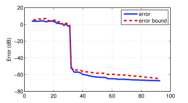
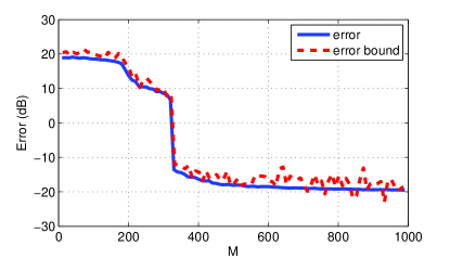
We show an example in Figure 8 where the true error appears along with a $90$-percent confidence bound. We have $N=1000$, $K=100$, $T=10$ and $\sigma_{n}=0.01$. We use basis pursuit denoising (12) as our choice for sparse solver, and we set $\lambda_{M}\propto\sqrt{M\log(N)}$ motivated by the universal rule for wavelet denoising [22] to account for noise added with additional measurements. The bound clearly shows where the sparse signal has been recovered up to the noise floor (the signal is sparse with $K=100$ non-zero elements).

Figure 8: Error estimate in the noisy case: true error and a $90$-percent confidence bound (dB scale): $N=1000$, $T=10$, $K=100$.

VII Efficient sequential solution

The main motivation for the sequential approach is to reduce the number of measurements to as few as possible. Yet, we would also like to keep the computational complexity of the sequential approach low. We focus on the $\ell_{1}$-based formulations here, and show that there is some potential of using ”memory” in the sequential setting for reducing the computational complexity. For the static setting there exists a great variety of approaches to solve both noiseless and noisy basis pursuit (i.e. basis pursuit denoising) in various forms, e.g. [23, 24, 25]. However, instead of re-solving the linear program (1) after each new sample, we would like to use the solution to the previous problem to guide the current problem. It is known that interior point methods are not well-suited to take advantage of such “warm-starts” [23]. Some methods are able to use warm-starts in the context of following the solution path in (11) as a function of $\lambda$ [23, 26, 27]. In that context the solution path $\hat{\mathbf{x}}(\lambda)$ is continuous (nearby values of $\lambda$ give nearby solutions) enabling warm-starts. However, once a new measurement ${\mathbf{a}}_{i}$ is received, this in general makes the previous solution infeasible, and can dramatically change the optimal solution, making warm-starts more challenging.

We now investigate a linear programming approach for warm-starts using the simplex method to accomplish this in the noiseless case (a similar strategy can be used with the Dantzig decoder [1] for the noisy case). We can not use the solution $\hat{\mathbf{x}}^{M}$ directly as a starting point for the new problem at step $M+1$, because in general it will not be feasible. In the Gaussian measurement case, unless $\hat{\mathbf{x}}^{M}={\mathbf{x}}^{*}$, the new constraint ${\mathbf{a}}_{M+1}^{\prime}\hat{\mathbf{x}}^{M}=y_{M+1}$ will be violated. One way to handle this is through a dual formulation, but we instead use an augmented primal formulation [29].

First, to model (1) as a linear program we use the standard trick: define $x_{i}^{+}=\max(x_{i},0)$, $x_{i}^{-}=\max(-x_{i},0)$, and ${\mathbf{x}}={\mathbf{x}}^{+}-{\mathbf{x}}^{-}$. This gives a linear program in standard form:

$$\min\boldsymbol{1}^{\prime}{\mathbf{x}}^{+}+\boldsymbol{1}^{\prime}{\mathbf{x}}^{-}$$ (13)

$${\mathbf{y}}_{1:M}=\left[A^{M}~{}~{}-A^{M}\right]\left[\begin{smallmatrix}{\mathbf{x}}^{+}\\ {\mathbf{x}}^{-}\end{smallmatrix}\right],~{}~{}\mbox{ and}~{}~{}{\mathbf{x}}^{+},{\mathbf{x}}^{-}\geq 0$$

Next we need to add an extra constraint $y_{M+1}={\mathbf{a}}_{M+1}^{\prime}{\mathbf{x}}^{+}-{\mathbf{a}}_{M+1}^{\prime}{\mathbf{x}}^{-}$. Suppose that ${\mathbf{a}}_{M+1}^{\prime}\hat{\mathbf{x}}^{M}>y_{M+1}$. We add an extra slack variable $z$ to the linear program, and a high positive cost $Q$ on $z$. This gives the following linear program:

$$\min\boldsymbol{1}^{\prime}{\mathbf{x}}^{+}+\boldsymbol{1}^{\prime}{\mathbf{x}}^{-}+Qz$$ (14)

$${\mathbf{y}}_{1:M}=\left[A^{M}~{}~{}-A^{M}\right]\left[\begin{smallmatrix}{\mathbf{x}}^{+}\\ {\mathbf{x}}^{-}\end{smallmatrix}\right],~{}~{}\mbox{ and}~{}~{}{\mathbf{x}}^{+},{\mathbf{x}}^{-}\geq 0$$

$$y_{M+1}={\mathbf{a}}_{M+1}^{\prime}{\mathbf{x}}^{+}-{\mathbf{a}}_{M+1}^{\prime}{\mathbf{x}}^{-}-z,~{}~{}\mbox{ and}~{}~{}z\geq 0$$

Now using $\hat{\mathbf{x}}^{M}$ and $z={\mathbf{a}}_{M+1}^{\prime}(\hat{\mathbf{x}}^{M})^{+}-{\mathbf{a}}_{M+1}^{\prime}(\hat{\mathbf{x}}^{M})^{-}-y_{M+1}$ yields a basic feasible solution to this augmented problem. By selecting $Q$ large enough, $z$ will be removed from the optimal basis (i.e. $z$ is set to $0$), and the solutions to this problem and the $(M+1)$-th sequential problem are the same.

Figure 9: A comparison of the number of simplex iterations when solving (1) from scratch (LP1) and using the solution at step $M-1$ (LP2). We plot the average number of iterations vs. $M$, over $100$ trials.

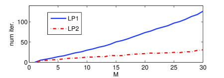
We test the approach on an example with $N=200$, $K=10$, and $100$ trials. In Figure 9 we plot the number of iterations of the simplex method required to solve the problem (1) at step $M$ from scratch (LP1) and using the formulation in (14) (LP2). To solve (13) we first have to find a basic feasible solution, BFS, (phase 1) and then move from it to the optimal BFS. An important advantage of (14) is that we start right away with a BFS, so phase 1 is not required. The figure illustrates that for large $M$ the approach LP2 is significantly faster.

We note that recently a very appealing approach for sequential solution in the noisy setting has been proposed based on the homotopy continuation idea [30, 31], where a homotopy (a continuous transition) is constructed from the problem at step $M$ to the problem at step $M+1$ and the piecewise-smooth path is followed. The efficiency of the approach depends on the number of break-points in this piecewise-smooth path, but the simulations results in the papers are very promising. We also note that [30] proposes an approach to select the trade-off in the noisy case, using cross-validation ideas.

VIII Conclusion and discussion

This paper presents a formulation for compressed sensing in which the decoder receives samples sequentially, and can perform computations in between samples. We showed how the decoder can estimate the error in the current reconstruction; this enables stopping once the error is within a required tolerance. Our results hold for any decoding algorithm, since they only depend on the distribution of the measurement vectors. This enables “run-time” performance guarantees in situations where a-priori guarantees may not be available, e.g. if the sparsity level of the signal is not known, or for recovery methods for which such guarantees have not been established.

We have studied a number of scenarios including noiseless, noisy, sparse and near sparse, and involving Gaussian and Bernoulli measurements, and demonstrated that the sequential approach is practical, flexible and has wide applicability. A very interesting problem is to both extend the results to other measurement ensembles, e.g. for sparse ensembles, and moreover, to go beyond results for particular ensembles and develop a general theory of sequential compressed sensing. Furthermore, in many important applications the sparse signal of interest may also be evolving with time during the measurement process. Sequential CS with a notion of ’time of a measurement’ is a natural candidate setting in which to explore this important extension to the CS literature.

We also remark that there is a closely related problem of recovering low-rank matrices from a small number of random measurements [32, 33], where instead of searching for sparse signals one looks for matrices with low-rank. This problem admits a convex ’nuclear-norm’ relaxation (much akin to $\ell_{1}$ relaxation of sparsity). Some of our results can be directly extended to this setting – for example if in the Gaussian measurement case with no noise there is one-step agreement, then the recovered low-rank matrix is the true low-rank solution with probability one.

Finally we comment on an important question [34, 6] of whether it is possible to do better than simply using random measurements – using e.g. experiment design or active learning techniques. In [6] the authors propose to find a multivariate Gaussian approximation to the posterior $p({\mathbf{x}}~{}|{\mathbf{y}})$ where $p({\mathbf{y}}~{}|~{}{\mathbf{x}})\propto\exp(\frac{1}{\sigma^{2}}\|{\mathbf{y}}-A{\mathbf{x}}\|^{2})$, and $p({\mathbf{x}})\propto\exp(-\lambda\|{\mathbf{x}}\|_{1})$. Note that MAP estimation in this model $\hat{\mathbf{x}}=\arg\max_{\mathbf{x}}p({\mathbf{x}}~{}|~{}{\mathbf{y}})$ is equivalent to the formulation in (11), but does not provide uncertainties. Using the Bayesian formalism it is possible to do experiment design, i.e. to select the next measurement to maximally reduce the expected uncertainty. This is a very exciting development, and although much more complex than the sequential approach presented here, may reduce the number of required samples even further.

Appendix A Derivation of the distribution for $\frac{1}{\sin{\theta}}$

Consider $E[\sin^{2}(\theta)]=E[\left(\sum_{i=1}^{T}h_{i}^{2}\right)/\|{\mathbf{h}}\|_{2}^{2}]$. Since $\sum_{i}E[\frac{h_{i}^{2}}{\|{\mathbf{h}}\|_{2}^{2}}]=1$, and each $h_{i}$ is i.i.d., we have $E[\frac{h_{i}^{2}}{\|{\mathbf{h}}\|_{2}^{2}}]=\frac{1}{L}$. In fact $E[\frac{h_{i}^{2}}{\|{\mathbf{h}}\|_{2}^{2}}]$ follows a Dirichlet distribution. Therefore, $E[\sin^{2}(\theta)]=\frac{T}{L}$.

Using Jensen’s inequality with the convex function $\sqrt{1/x}$, $x>0$, we have $E[1/\sin(\theta)]\geq\sqrt{\frac{L}{T}}$.

Now, $E[\frac{1}{\sin^{2}(\theta)}]=\frac{L-2}{T-2}$ (for $T>2$). This is true because $E[\frac{1}{\sin^{2}(\theta)}]=E\left(\sum_{i=1}^{L}h_{i}^{2}\right)/\left(\sum_{i=1}^{T}h_{i}^{2}\right)=$ $1+E\left(\sum_{i={T+1}}^{L}h_{i}^{2}/\sum_{i=1}^{T}h_{i}^{2}\right)=1+(L-T)\frac{1}{T-2}$. The second term is a product of a $\chi^{2}$ random variable with $(L-T)$ degrees of freedom and an independent inverse-$\chi^{2}$ distribution with $T$ degrees of freedom: $E[\sum_{i={T+1}}^{L}h_{i}^{2}]=L-T$, and $E[\frac{1}{\left(\sum_{i=1}^{T}h_{i}^{2}\right)}]=\frac{1}{T-2}$, see [20]. Now $1+(L-T)/(T-2)=(L-2)/(T-2)$.

Finally, using Jensen’s inequality with the concave function $\sqrt{x}$, $E[\frac{1}{\sin(\theta)}]\leq\sqrt{\frac{T-2}{L-2}}$.

References

- [1] E. J. Candes, “Compressive sampling,” in Proc. Int. Congress of Math., 2006, Madrid, Spain.
- [2] D. Donoho, “Compressed sensing,” IEEE Trans. on Information Theory, vol. 52, no. 4, pp. 1289–1306, Apr. 2006.
- [3] M. Lustig, D. L. Donoho, and J. M. Pauly, “Sparse MRI: The application of compressed sensing for rapid MR imaging,” Magnetic Resonance in Medicine, vol. 58, no. 6, pp. 1182–1195, Dec. 2007.
- [4] M. F. Duarte, M. A. Davenport, D. Takhar, J. N. Laska, T. Sun, K. F. Kelly, and R. Baraniuk, “Single pixel imaging via compressive sampling,” IEEE Signal Processing Magazine, vol. 25, no. 2, pp. 83–91, Mar. 2008.
- [5] W. Bajwa, J. Haupt, A. Sayeed, and R. Nowak, “Compressive wireless sensing,” in Int. Conf. on Information Processing in Sensor Networks (IPSN), April 2006.
- [6] F. Steinke, M. Seeger, and K. Tsuda, “Experimental design for efficient identification of gene regulatory networks using sparse Bayesian models,” BMC Systems Biology, vol. 1, no. 51, 2007.
- [7] S. S. Chen, D. L. Donoho, and M. A. Saunders, “Atomic decomposition by basis pursuit,” SIAM J. Scientific Computing, vol. 20, no. 1, pp. 33–61, 1998.
- [8] J. Tropp, “Greed is good: Algorithmic results for sparse approximation,” IEEE Trans. Info. Theory, vol. 50, no. 10, pp. 2231–2242, Oct. 2004.
- [9] R. Chartrand and W. Yin, “Iteratively reweighted algorithms for compressive sensing,” in ICASSP, 2008.
- [10] M. Cetin, D. M. Malioutov, and A. S. Willsky, “A variational technique for source localization based on a sparse signal reconstruction perspective,” in ICASSP, 2002.
- [11] E. J. Candes, M. Wakin, and S. Boyd, “Enhancing sparsity by reweighted l1 minimization,” 2007, technical report, California Institute of Technology.
- [12] E. Cand s, J. Romberg, and T. Tao, “Robust uncertainty principles: Exact signal reconstruction from highly incomplete frequency information,” IEEE Trans. on Information Theory, vol. 52, no. 2, pp. 489–509, Feb. 2006.
- [13] D. Wipf and B. D. Rao, “Sparse bayesian learning for basis selection,” IEEE Transactions on Signal Processing, vol. 52, no. 8, 2004.
- [14] M. Rudelson and R. Vershynin, “Sparse reconstruction by convex relaxation: Fourier and Gaussian measurements,” in CISS 2006, 2006.
- [15] R. Ward, “Compressed sensing with cross validation,” to appear in IEEE Transactions on Information Theory, 2009.
- [16] D. M. Malioutov, S. R. Sanghavi, and A. S. Willsky, “Compressed sensing with sequential observations,” in ICASSP, 2008.
- [17] R. Baraniuk, “Compressive sensing,” IEEE Signal Processing Magazine, vol. 24, no. 4, pp. 118–121, Jul. 2007.
- [18] D. L. Donoho and X. Huo, “Uncertainty principles and ideal atomic decomposition,” IEEE Trans. on Information Theory, vol. 47, no. 7, pp. 2845–2862, Nov. 2001.
- [19] T. Tao and V. Vu, “On the singularity probability of random Bernoulli matrices,” Journal Amer. Math. Soc., vol. 20, pp. 603–628, 2007.
- [20] S. Kotz, N. Balakrishnan, and N. L. Johnson, Continuous Multivariate Distributions. Wiley and Sons, 2000.
- [21] S. Dasgupta and A. Gupta, “An elementary proof of a theorem of Johnson and Lindenstrauss,” Random Structures and Algorithms, 22(1):60-65, vol. 22, no. 1, pp. 60–65, 2003.
- [22] I. M. J. D. L. Donoho, “Ideal spatial adaptation by wavelet shrinkage,” Biometrika, vol. 81, no. 3, pp. 425–455, 1994.
- [23] M. Figueiredo, R. Nowak, and S. Wright, “Gradient projection for sparse reconstruction: application to compressed sensing and other inverse problems,” IEEE Journal of Selected Topics in Signal Processing, vol. 1, no. 4, pp. 586–598, 2007.
- [24] S. J. Kim, K. Koh, M. Lustig, S. Boyd, and D. Gorinevsky, “A method for large-scale l1-regularized least squares,” IEEE Journal on Selected Topics in Signal Processing, vol. 4, no. 1, pp. 606–617, Dec. 2007.
- [25] I. Daubechies, M. De Friese, and C. De Mol, “An iterative thresholding algorithm for linear inverse problems with a sparsity constraint,” Comm. in Pure and Applied Math., vol. 57, pp. 1413–1457, 2004.
- [26] M. R. Osborne, B. Presnell, and B. A. Turlach, “A new approach to variable selection in least squares problems,” IMA Journal of Numerical Analysis, vol. 20, no. 3, pp. 389–403, 2000.
- [27] D. M. Malioutov, M. Cetin, and A. S. Willsky, “Homotopy continuation for sparse signal representation,” in ICASSP, 2005.
- [28] S. Sra and J. A. Tropp, “Row-action methods for compressed sensing,” in ICASSP, vol. 3, 2006, pp. 868–871.
- [29] D. Bertsimas and J. N. Tsitsiklis, Introduction to linear optimization. Athena Scientific, 1997.
- [30] P. J. Garrigues and L. El Ghaoui, “An homotopy algorithm for the Lasso with online observations,” in Neural Information Processing Systems (NIPS), Dec. 2008.
- [31] M. S. Asif and J. Romberg, “Streaming measurements in compressive sensing: L1 filtering,” in Proc. of 42nd Asilomar Conference on Signals, Systems and Computers, Oct. 2008.
- [32] B. Recht, M. Fazel, and P. A. Parrilo, “Guaranteed minimum rank solutions to linear matrix equations via nuclear norm minimization,” submitted to SIAM Review, 2007.
- [33] R. Keshavan, A. Montanari, and S. Oh, “Learning low rank matrices from O(n) entries,” in Allerton Conference., Oct. 2008.
- [34] Y. Weiss, H. S. Chang, and W. T. Freeman, “Learning compressed sensing,” in Allerton Conference, Sep. 2007.