A Contextual-Bandit Approach to
Personalized News Article Recommendation
Abstract
Personalized web services strive to adapt their services (advertisements, news articles, etc.) to individual users by making use of both content and user information. Despite a few recent advances, this problem remains challenging for at least two reasons. First, web service is featured with dynamically changing pools of content, rendering traditional collaborative filtering methods inapplicable. Second, the scale of most web services of practical interest calls for solutions that are both fast in learning and computation.
In this work, we model personalized recommendation of news articles as a contextual bandit problem, a principled approach in which a learning algorithm sequentially selects articles to serve users based on contextual information about the users and articles, while simultaneously adapting its article-selection strategy based on user-click feedback to maximize total user clicks.
The contributions of this work are three-fold. First, we propose a new, general contextual bandit algorithm that is computationally efficient and well motivated from learning theory. Second, we argue that any bandit algorithm can be reliably evaluated offline using previously recorded random traffic. Finally, using this offline evaluation method, we successfully applied our new algorithm to a Yahoo! Front Page Today Module dataset containing over million events. Results showed a click lift compared to a standard context-free bandit algorithm, and the advantage becomes even greater when data gets more scarce.
category:
H.3.5 Information Systems On-line Information Servicescategory:
I.2.6 Computing Methodologies Learningkeywords:
Contextual bandit, web service, personalization, recommender systems, exploration/exploitation dilemma1 Introduction
This paper addresses the challenge of identifying the most appropriate web-based content at the best time for individual users. Most service vendors acquire and maintain a large amount of content in their repository, for instance, for filtering news articles [14] or for the display of advertisements [5]. Moreover, the content of such a web-service repository changes dynamically, undergoing frequent insertions and deletions. In such a setting, it is crucial to quickly identify interesting content for users. For instance, a news filter must promptly identify the popularity of breaking news, while also adapting to the fading value of existing, aging news stories.
It is generally difficult to model popularity and temporal changes based solely on content information. In practice, we usually explore the unknown by collecting consumers’ feedback in real time to evaluate the popularity of new content while monitoring changes in its value [3]. For instance, a small amount of traffic can be designated for such exploration. Based on the users’ response (such as clicks) to randomly selected content on this small slice of traffic, the most popular content can be identified and exploited on the remaining traffic. This strategy, with random exploration on an fraction of the traffic and greedy exploitation on the rest, is known as -greedy. Advanced exploration approaches such as EXP3 [8] or UCB1 [7] could be applied as well. Intuitively, we need to distribute more traffic to new content to learn its value more quickly, and fewer users to track temporal changes of existing content.
Recently, personalized recommendation has become a desirable feature for websites to improve user satisfaction by tailoring content presentation to suit individual users’ needs [10]. Personalization involves a process of gathering and storing user attributes, managing content assets, and, based on an analysis of current and past users’ behavior, delivering the individually best content to the present user being served.
Often, both users and content are represented by sets of features. User features may include historical activities at an aggregated level as well as declared demographic information. Content features may contain descriptive information and categories. In this scenario, exploration and exploitation have to be deployed at an individual level since the views of different users on the same content can vary significantly. Since there may be a very large number of possible choices or actions available, it becomes critical to recognize commonalities between content items and to transfer that knowledge across the content pool.
Traditional recommender systems, including collaborative filtering, content-based filtering and hybrid approaches, can provide meaningful recommendations at an individual level by leveraging users’ interests as demonstrated by their past activity. Collaborative filtering [25], by recognizing similarities across users based on their consumption history, provides a good recommendation solution to the scenarios where overlap in historical consumption across users is relatively high and the content universe is almost static. Content-based filtering helps to identify new items which well match an existing user’s consumption profile, but the recommended items are always similar to the items previously taken by the user [20]. Hybrid approaches [11] have been developed by combining two or more recommendation techniques; for example, the inability of collaborative filtering to recommend new items is commonly alleviated by combining it with content-based filtering.
However, as noted above, in many web-based scenarios, the content universe undergoes frequent changes, with content popularity changing over time as well. Furthermore, a significant number of visitors are likely to be entirely new with no historical consumption record whatsoever; this is known as a cold-start situation [21]. These issues make traditional recommender-system approaches difficult to apply, as shown by prior empirical studies [12]. It thus becomes indispensable to learn the goodness of match between user interests and content when one or both of them are new. However, acquiring such information can be expensive and may reduce user satisfaction in the short term, raising the question of optimally balancing the two competing goals: maximizing user satisfaction in the long run, and gathering information about goodness of match between user interests and content.
The above problem is indeed known as a feature-based exploration/exploitation problem. In this paper, we formulate it as a contextual bandit problem, a principled approach in which a learning algorithm sequentially selects articles to serve users based on contextual information of the user and articles, while simultaneously adapting its article-selection strategy based on user-click feedback to maximize total user clicks in the long run. We define a bandit problem and then review some existing approaches in Section 2. Then, we propose a new algorithm, LinUCB, in Section 3 which has a similar regret analysis to the best known algorithms for competing with the best linear predictor, with a lower computational overhead. We also address the problem of offline evaluation in Section 4, showing this is possible for any explore/exploit strategy when interactions are independent and identically distributed (i.i.d.), as might be a reasonable assumption for different users. We then test our new algorithm and several existing algorithms using this offline evaluation strategy in Section 5.
2 Formulation & Related Work
In this section, we define the -armed contextual bandit problem formally, and as an example, show how it can model the personalized news article recommendation problem. We then discuss existing methods and their limitations.
2.1 A Multi-armed Bandit Formulation
The problem of personalized news article recommendation can be naturally modeled as a multi-armed bandit problem with context information. Following previous work [18], we call it a contextual bandit.111In the literature, contextual bandits are sometimes called bandits with covariate, bandits with side information, associative bandits, and associative reinforcement learning. Formally, a contextual-bandit algorithm proceeds in discrete trials In trial :
-
1.
The algorithm observes the current user and a set of arms or actions together with their feature vectors for . The vector summarizes information of both the user and arm , and will be referred to as the context.
-
2.
Based on observed payoffs in previous trials, chooses an arm , and receives payoff whose expectation depends on both the user and the arm .
-
3.
The algorithm then improves its arm-selection strategy with the new observation, . It is important to emphasize here that no feedback (namely, the payoff ) is observed for unchosen arms . The consequence of this fact is discussed in more details in the next subsection.
In the process above, the total -trial payoff of is defined as Similarly, we define the optimal expected -trial payoff as where is the arm with maximum expected payoff at trial . Our goal is to design so that the expected total payoff above is maximized. Equivalently, we may find an algorithm so that its regret with respect to the optimal arm-selection strategy is minimized. Here, the -trial regret of algorithm is defined formally by
| (1) |
An important special case of the general contextual bandit problem is the well-known -armed bandit in which (i) the arm set remains unchanged and contains arms for all , and (ii) the user (or equivalently, the context ) is the same for all . Since both the arm set and contexts are constant at every trial, they make no difference to a bandit algorithm, and so we will also refer to this type of bandit as a context-free bandit.
In the context of article recommendation, we may view articles in the pool as arms. When a presented article is clicked, a payoff of is incurred; otherwise, the payoff is . With this definition of payoff, the expected payoff of an article is precisely its click-through rate (CTR), and choosing an article with maximum CTR is equivalent to maximizing the expected number of clicks from users, which in turn is the same as maximizing the total expected payoff in our bandit formulation.
Furthermore, in web services we often have access to user information which can be used to infer a user’s interest and to choose news articles that are probably most interesting to her. For example, it is much more likely for a male teenager to be interested in an article about iPod products rather than retirement plans. Therefore, we may “summarize” users and articles by a set of informative features that describe them compactly. By doing so, a bandit algorithm can generalize CTR information from one article/user to another, and learn to choose good articles more quickly, especially for new users and articles.
2.2 Existing Bandit Algorithms
The fundamental challenge in bandit problems is the need for balancing exploration and exploitation. To minimize the regret in Eq. (1), an algorithm exploits its past experience to select the arm that appears best. On the other hand, this seemingly optimal arm may in fact be suboptimal, due to imprecision in ’s knowledge. In order to avoid this undesired situation, has to explore by actually choosing seemingly suboptimal arms so as to gather more information about them (c.f., step 3 in the bandit process defined in the previous subsection). Exploration can increase short-term regret since some suboptimal arms may be chosen. However, obtaining information about the arms’ average payoffs (i.e., exploration) can refine ’s estimate of the arms’ payoffs and in turn reduce long-term regret. Clearly, neither a purely exploring nor a purely exploiting algorithm works best in general, and a good tradeoff is needed.
The context-free -armed bandit problem has been studied by statisticians for a long time [9, 24, 26]. One of the simplest and most straightforward algorithms is -greedy. In each trial , this algorithm first estimates the average payoff of each arm . Then, with probability , it chooses the greedy arm (i.e., the arm with highest payoff estimate); with probability , it chooses a random arm. In the limit, each arm will be tried infinitely often, and so the payoff estimate converges to the true value with probability . Furthermore, by decaying appropriately (e.g., [24]), the per-step regret, , converges to with probability .
In contrast to the unguided exploration strategy adopted by -greedy, another class of algorithms generally known as upper confidence bound algorithms [4, 7, 17] use a smarter way to balance exploration and exploitation. Specifically, in trial , these algorithms estimate both the mean payoff of each arm as well as a corresponding confidence interval , so that holds with high probability. They then select the arm that achieves a highest upper confidence bound (UCB for short): . With appropriately defined confidence intervals, it can be shown that such algorithms have a small total -trial regret that is only logarithmic in the total number of trials , which turns out to be optimal [17].
While context-free -armed bandits are extensively studied and well understood, the more general contextual bandit problem has remained challenging. The EXP4 algorithm [8] uses the exponential weighting technique to achieve an regret,222Note is the same as but suppresses logarithmic factors. but the computational complexity may be exponential in the number of features. Another general contextual bandit algorithm is the epoch-greedy algorithm [18] that is similar to -greedy with shrinking . This algorithm is computationally efficient given an oracle optimizer but has the weaker regret guarantee of .
Algorithms with stronger regret guarantees may be designed under various modeling assumptions about the bandit. Assuming the expected payoff of an arm is linear in its features, Auer [6] describes the LinRel algorithm that is essentially a UCB-type approach and shows that one of its variants has a regret of , a significant improvement over earlier algorithms [1].
Finally, we note that there exist another class of bandit algorithms based on Bayes rule, such as Gittins index methods [15]. With appropriately defined prior distributions, Bayesian approaches may have good performance. These methods require extensive offline engineering to obtain good prior models, and are often computationally prohibitive without coupling with approximation techniques [2].
3 Algorithm
Given asymptotic optimality and the strong regret bound of UCB methods for context-free bandit algorithms, it is tempting to devise similar algorithms for contextual bandit problems. Given some parametric form of payoff function, a number of methods exist to estimate from data the confidence interval of the parameters with which we can compute a UCB of the estimated arm payoff. Such an approach, however, is expensive in general.
In this work, we show that a confidence interval can be computed efficiently in closed form when the payoff model is linear, and call this algorithm LinUCB. For convenience of exposition, we first describe the simpler form for disjoint linear models, and then consider the general case of hybrid models in Section 3.2. We note LinUCB is a generic contextual bandit algorithms which applies to applications other than personalized news article recommendation.
3.1 LinUCB with Disjoint Linear Models
Using the notation of Section 2.1, we assume the expected payoff of an arm is linear in its -dimensional feature with some unknown coefficient vector ; namely, for all ,
| (2) |
This model is called disjoint since the parameters are not shared among different arms. Let be a design matrix of dimension at trial , whose rows correspond to training inputs (e.g., contexts that are observed previously for article ), and be the corresponding response vector (e.g., the corresponding click/no-click user feedback). Applying ridge regression to the training data gives an estimate of the coefficients:
| (3) |
where is the identity matrix. When components in are independent conditioned on corresponding rows in , it can be shown [27] that, with probability at least ,
| (4) |
for any and , where is a constant. In other words, the inequality above gives a reasonably tight UCB for the expected payoff of arm , from which a UCB-type arm-selection strategy can be derived: at each trial , choose
| (5) |
where .
The confidence interval in Eq. (4) may be motivated and derived from other principles. For instance, ridge regression can also be interpreted as a Bayesian point estimate, where the posterior distribution of the coefficient vector, denoted as , is Gaussian with mean and covariance . Given the current model, the predictive variance of the expected payoff is evaluated as , and then becomes the standard deviation. Furthermore, in information theory [19], the differential entropy of is defined as . The entropy of when updated by the inclusion of the new point then becomes . The entropy reduction in the model posterior is . This quantity is often used to evaluate model improvement contributed from . Therefore, the criterion for arm selection in Eq. (5) can also be regarded as an additive trade-off between the payoff estimate and model uncertainty reduction.
Algorithm 1 gives a detailed description of the entire LinUCB algorithm, whose only input parameter is . Note the value of given in Eq. (4) may be conservatively large in some applications, and so optimizing this parameter may result in higher total payoffs in practice. Like all UCB methods, LinUCB always chooses the arm with highest UCB (as in Eq. (5)).
This algorithm has a few nice properties. First, its computational complexity is linear in the number of arms and at most cubic in the number of features. To decrease computation further, we may update in every step (which takes time), but compute and cache (for all ) periodically instead of in real-time. Second, the algorithm works well for a dynamic arm set, and remains efficient as long as the size of is not too large. This case is true in many applications. In news article recommendation, for instance, editors add/remove articles to/from a pool and the pool size remains essentially constant. Third, although it is not the focus of the present paper, we can adapt the analysis from [6] to show the following: if the arm set is fixed and contains arms, then the confidence interval (i.e., the right-hand side of Eq. (4)) decreases fast enough with more and more data, and then prove the strong regret bound of , matching the state-of-the-art result [6] for bandits satisfying Eq. (2). These theoretical results indicate fundamental soundness and efficiency of the algorithm.
Finally, we note that, under the assumption that input features were drawn i.i.d. from a normal distribution (in addition to the modeling assumption in Eq. (2)), Pavlidis et al. [22] came up with a similar algorithm that uses a least-squares solution instead of our ridge-regression solution ( in Eq. (3)) to compute the UCB. However, our approach (and theoretical analysis) is more general and remains valid even when input features are nonstationary. More importantly, we will discuss in the next section how to extend the basic Algorithm 1 to a much more interesting case not covered by Pavlidis et al.
3.2 LinUCB with Hybrid Linear Models
Algorithm 1 (or the similar algorithm in [22]) computes the inverse of the matrix, (or ), where is again the design matrix with rows corresponding to features in the training data. These matrices of all arms have fixed dimension , and can be updated efficiently and incrementally. Moreover, their inverses can be computed easily as the parameters in Algorithm 1 are disjoint: the solution in Eq. (3) is not affected by training data of other arms, and so can be computed separately. We now consider the more interesting case with hybrid models.
In many applications including ours, it is helpful to use features that are shared by all arms, in addition to the arm-specific ones. For example, in news article recommendation, a user may prefer only articles about politics for which this provides a mechanism. Hence, it is helpful to have features that have both shared and non-shared components. Formally, we adopt the following hybrid model by adding another linear term to the right-hand side of Eq. (2):
| (6) |
where is the feature of the current user/article combination, and is an unknown coefficient vector common to all arms. This model is hybrid in the sense that some of the coefficients are shared by all arms, while others are not.
For hybrid models, we can no longer use Algorithm 1 as the confidence intervals of various arms are not independent due to the shared features. Fortunately, there is an efficient way to compute an UCB along the same line of reasoning as in the previous section. The derivation relies heavily on block matrix inversion techniques. Due to space limitation, we only give the pseudocode in Algorithm 2 (where lines 5 and 12 compute the ridge-regression solution of the coefficients, and line 13 computes the confidence interval), and leave detailed derivations to a full paper. Here, we only point out the important fact that the algorithm is computationally efficient since the building blocks in the algorithm (, , , , and ) all have fixed dimensions and can be updated incrementally. Furthermore, quantities associated with arms not existing in no longer get involved in the computation. Finally, we can also compute and cache the inverses ( and ) periodically instead of at the end of each trial to reduce the per-trial computational complexity to .
4 Evaluation Methodology
Compared to machine learning in the more standard supervised setting, evaluation of methods in a contextual bandit setting is frustratingly difficult. Our goal here is to measure the performance of a bandit algorithm , that is, a rule for selecting an arm at each time step based on the preceding interactions (such as the algorithms described above). Because of the interactive nature of the problem, it would seem that the only way to do this is to actually run the algorithm on “live” data. However, in practice, this approach is likely to be infeasible due to the serious logistical challenges that it presents. Rather, we may only have offline data available that was collected at a previous time using an entirely different logging policy. Because payoffs are only observed for the arms chosen by the logging policy, which are likely to often differ from those chosen by the algorithm being evaluated, it is not at all clear how to evaluate based only on such logged data. This evaluation problem may be viewed as a special case of the so-called “off-policy evaluation problem” in reinforcement learning (see, c.f., [23]).
One solution is to build a simulator to model the bandit process from the logged data, and then evaluate with the simulator. However, the modeling step will introduce bias in the simulator and so make it hard to justify the reliability of this simulator-based evaluation approach. In contrast, we propose an approach that is simple to implement, grounded on logged data, and unbiased.
In this section, we describe a provably reliable technique for carrying out such an evaluation, assuming that the individual events are i.i.d., and that the logging policy that was used to gather the logged data chose each arm at each time step uniformly at random. Although we omit the details, this latter assumption can be weakened considerably so that any randomized logging policy is allowed and our solution can be modified accordingly using rejection sampling, but at the cost of decreased efficiency in using data.
More precisely, we suppose that there is some unknown distribution from which tuples are drawn i.i.d. of the form , each consisting of observed feature vectors and hidden payoffs for all arms. We also posit access to a large sequence of logged events resulting from the interaction of the logging policy with the world. Each such event consists of the context vectors , a selected arm and the resulting observed payoff . Crucially, only the payoff is observed for the single arm that was chosen uniformly at random. For simplicity of presentation, we take this sequence of logged events to be an infinitely long stream; however, we also give explicit bounds on the actual finite number of events required by our evaluation method.
Our goal is to use this data to evaluate a bandit algorithm . Formally, is a (possibly randomized) mapping for selecting the arm at time based on the history of preceding events, together with the current context vectors .
Our proposed policy evaluator is shown in Algorithm 3. The method takes as input a policy and a desired number of “good” events on which to base the evaluation. We then step through the stream of logged events one by one. If, given the current history , it happens that the policy chooses the same arm as the one that was selected by the logging policy, then the event is retained, that is, added to the history, and the total payoff updated. Otherwise, if the policy selects a different arm from the one that was taken by the logging policy, then the event is entirely ignored, and the algorithm proceeds to the next event without any other change in its state.
Note that, because the logging policy chooses each arm uniformly at random, each event is retained by this algorithm with probability exactly , independent of everything else. This means that the events which are retained have the same distribution as if they were selected by . As a result, we can prove that two processes are equivalent: the first is evaluating the policy against real-world events from , and the second is evaluating the policy using the policy evaluator on a stream of logged events.
Theorem 1
For all distributions of contexts, all policies , all , and all sequences of events ,
where is a stream of events drawn i.i.d. from a uniform random logging policy and . Furthermore, the expected number of events obtained from the stream to gather a history of length is .
This theorem says that every history has the identical probability in the real world as in the policy evaluator. Many statistics of these histories, such as the average payoff returned by Algorithm 3, are therefore unbiased estimates of the value of the algorithm . Further, the theorem states that logged events are required, in expectation, to retain a sample of size .
Proof 4.2.
The proof is by induction on starting with a base case of the empty history which has probability when under both methods of evaluation. In the inductive case, assume that we have for all :
and want to prove the same statement for any history . Since the data is i.i.d. and any randomization in the policy is independent of randomization in the world, we need only prove that conditioned on the history the distribution over the -th event is the same for each process. In other words, we must show:
Since the arm is chosen uniformly at random in the logging policy, the probability that the policy evaluator exits the inner loop is identical for any policy, any history, any features, and any arm, implying this happens for the last event with the probability of the last event, . Similarly, since the policy ’s distribution over arms is independent conditioned on the history and features , the probability of arm is just .
Finally, since each event from the stream is retained with probability exactly , the expected number required to retain events is exactly .
5 Experiments
In this section, we verify the capacity of the proposed LinUCB algorithm on a real-world application using the offline evaluation method of Section 4. We start with an introduction of the problem setting in Yahoo! Today-Module, and then describe the user/item attributes we used in experiments. Finally, we define performance metrics and report experimental results with comparison to a few standard (contextual) bandit algorithms.

5.1 Yahoo! Today Module
The Today Module is the most prominent panel on the Yahoo! Front Page, which is also one of the most visited pages on the Internet; see a snapshot in Figure 1. The default “Featured” tab in the Today Module highlights one of four high-quality articles, mainly news, while the four articles are selected from an hourly-refreshed article pool curated by human editors. As illustrated in Figure 1, there are four articles at footer positions, indexed by F1–F4. Each article is represented by a small picture and a title. One of the four articles is highlighted at the story position, which is featured by a large picture, a title and a short summary along with related links. By default, the article at F1 is highlighted at the story position. A user can click on the highlighted article at the story position to read more details if she is interested in the article. The event is recorded as a story click. To draw visitors’ attention, we would like to rank available articles according to individual interests, and highlight the most attractive article for each visitor at the story position.
5.2 Experiment Setup
| algorithm | size = 100% | size = 30% | size = 20% | size = 10% | size = 5% | size = 1% | ||||||
|---|---|---|---|---|---|---|---|---|---|---|---|---|
| deploy | learn | deploy | learn | deploy | learn | deploy | learn | deploy | learn | deploy | learn | |
| -greedy | ||||||||||||
| % | % | % | % | % | % | % | % | % | % | % | % | |
| ucb | ||||||||||||
| % | % | % | % | % | % | % | % | % | % | % | % | |
| -greedy (seg) | ||||||||||||
| % | % | % | % | % | % | % | % | % | % | % | % | |
| ucb (seg) | ||||||||||||
| % | % | % | % | % | % | % | % | % | % | % | % | |
| -greedy (disjoint) | ||||||||||||
| % | % | % | % | % | % | % | % | % | % | % | % | |
| linucb (disjoint) | ||||||||||||
| % | % | % | % | % | % | % | % | % | % | % | % | |
| -greedy (hybrid) | ||||||||||||
| % | % | % | % | % | % | % | % | % | % | % | % | |
| linucb (hybrid) | ||||||||||||
| % | % | % | % | % | % | % | % | % | % | % | % | |
This subsection gives a detailed description of our experimental setup, including data collection, feature construction, performance evaluation, and competing algorithms.
5.2.1 Data Collection
We collected events from a random bucket in May 2009. Users were randomly selected to the bucket with a certain probability per visiting view.333We call it view-based randomization. After refreshing her browser, the user may not fall into the random bucket again. In this bucket, articles were randomly selected from the article pool to serve users. To avoid exposure bias at footer positions, we only focused on users’ interactions with F1 articles at the story position. Each user interaction event consists of three components: (i) the random article chosen to serve the user, (ii) user/article information, and (iii) whether the user clicks on the article at the story position. Section 4 shows these random events can be used to reliably evaluate a bandit algorithm’s expected payoff.
There were about million events in the random bucket on May 01. We used this day’s events (called “tuning data”) for model validation to decide the optimal parameter for each competing bandit algorithm. Then we ran these algorithms with tuned parameters on a one-week event set (called “evaluation data”) in the random bucket from May 03–09, which contained about million events.
5.2.2 Feature Construction
We now describe the user/article features constructed for our experiments. Two sets of features for the disjoint and hybrid models, respectively, were used to test the two forms of LinUCB in Section 3 and to verify our conjecture that hybrid models can improve learning speed.
We start with raw user features that were selected by “support”. The support of a feature is the fraction of users having that feature. To reduce noise in the data, we only selected features with high support. Specifically, we used a feature when its support is at least . Then, each user was originally represented by a raw feature vector of over categorical components, which include: (i) demographic information: gender ( classes) and age discretized into segments; (ii) geographic features: about metropolitan locations worldwide and U.S. states; and (iii) behavioral categories: about binary categories that summarize the user’s consumption history within Yahoo! properties. Other than these features, no other information was used to identify a user.
Similarly, each article was represented by a raw feature vector of about categorical features constructed in the same way. These features include: (i) URL categories: tens of classes inferred from the URL of the article resource; and (ii) editor categories: tens of topics tagged by human editors to summarize the article content.
We followed a previous procedure [12] to encode categorical user/article features as binary vectors and then normalize each feature vector to unit length. We also augmented each feature vector with a constant feature of value . Now each article and user was represented by a feature vector of and entries, respectively.
To further reduce dimensionality and capture nonlinearity in these raw features, we carried out conjoint analysis based on random exploration data collected in September 2008. Following a previous approach to dimensionality reduction [13], we projected user features onto article categories and then clustered users with similar preferences into groups. More specifically:
-
•
We first used logistic regression (LR) to fit a bilinear model for click probability given raw user/article features so that approximated the probability that the user clicks on article , where and were the corresponding feature vectors, and was a weight matrix optimized by LR.
-
•
Raw user features were then projected onto an induced space by computing . Here, the component in for user may be interpreted as the degree to which the user likes the category of articles. K-means was applied to group users in the induced space into clusters.
-
•
The final user feature was a six-vector: five entries corresponded to membership of that user in these clusters (computed with a Gaussian kernel and then normalized so that they sum up to unity), and the sixth was a constant feature .
At trial , each article has a separate six-dimensional feature that is exactly the six-dimensional feature constructed as above for user . Since these article features do not overlap, they are for disjoint linear models defined in Section 3.
For each article , we performed the same dimensionality reduction to obtain a six-dimensional article feature (including a constant feature). Its outer product with a user feature gave features, denoted , that corresponded to the shared features in Eq. (6), and thus could be used in the hybrid linear model. Note the features contains user-article interaction information, while contains user information only.
Here, we intentionally used five users (and articles) groups, which has been shown to be representative in segmentation analysis [13]. Another reason for using a relatively small feature space is that, in online services, storing and retrieving large amounts of user/article information will be too expensive to be practical.
5.3 Compared Algorithms
The algorithms empirically evaluated in our experiments can be categorized into three groups:
I. Algorithms that make no use of features. These correspond to the context-free -armed bandit algorithms that ignore all contexts (i.e., user/article information).
-
•
random: A random policy always chooses one of the candidate articles from the pool with equal probability. This algorithm requires no parameters and does not “learn” over time.
-
•
-greedy: As described in Section 2.2, it estimates each article’s CTR; then it chooses a random article with probability , and chooses the article of the highest CTR estimate with probability . The only parameter of this policy is .
-
•
ucb: As described in Section 2.2, this policy estimates each article’s CTR as well as a confidence interval of the estimate, and always chooses the article with the highest UCB. Specifically, following UCB1 [7], we computed an article ’s confidence interval by , where is the number of times was chosen prior to trial , and is a parameter.
-
•
omniscient: Such a policy achieves the best empirical context-free CTR from hindsight. It first computes each article’s empirical CTR from logged events, and then always chooses the article with highest empircal CTR when it is evaluated using the same logged events. This algorithm requires no parameters and does not “learn” over time.
II. Algorithms with “warm start”—an intermediate step towards personalized services. The idea is to provide an offline-estimated user-specific adjustment on articles’ context-free CTRs over the whole traffic. The offset serves as an initialization on CTR estimate for new content, a.k.a.“warm start”. We re-trained the bilinear logistic regression model studied in [12] on Sept 2008 random traffic data, using features constructed above. The selection criterion then becomes the sum of the context-free CTR estimate and a bilinear term for a user-specific CTR adjustment. In training, CTR was estimated using the context-free -greedy with .
-
•
-greedy (warm): This algorithm is the same as -greedy except it adds the user-specific CTR correction to the article’s context-free CTR estimate.
-
•
ucb (warm): This algorithm is the same as the previous one but replaces -greedy with ucb.
III. Algorithms that learn user-specific CTRs online.
-
•
-greedy (seg): Each user is assigned to the closest user cluster among the five constructed in Section 5.2.2, and so all users are partitioned into five groups (a.k.a. user segments), in each of which a separate copy of -greedy was run.
-
•
ucb (seg): This algorithm is similar to -greedy (seg) except it ran a copy of ucb in each of the five user segments.
-
•
-greedy (disjoint): This is -greedy with disjoint models, and may be viewed as a close variant of epoch-greedy [18].
-
•
linucb (disjoint): This is Algorithm 1 with disjoint models.
-
•
-greedy (hybrid): This is -greedy with hybrid models, and may be viewed as a close variant of epoch-greedy.
-
•
linucb (hybrid): This is Algorithm 2 with hybrid models.
5.4 Performance Metric
An algorithm’s CTR is defined as the ratio of the number of clicks it receives and the number of steps it is run. We used all algorithms’ CTRs on the random logged events for performance comparison. To protect business-sensitive information, we report an algorithm’s relative CTR, which is the algorithm’s CTR divided by the random policy’s. Therefore, we will not report a random policy’s relative CTR as it is always by definition. For convenience, we will use the term “CTR” from now on instead of “relative CTR”.
For each algorithm, we are interested in two CTRs motivated by our application, which may be useful for other similar applications. When deploying the methods to Yahoo!’s front page, one reasonable way is to randomly split all traffic to this page into two buckets [3]. The first, called “learning bucket”, usually consists of a small fraction of traffic on which various bandit algorithms are run to learn/estimate article CTRs. The other, called “deployment bucket”, is where Yahoo! Front Page greedily serves users using CTR estimates obained from the learning bucket. Note that “learning” and “deployment” are interleaved in this problem, and so in every view falling into the deployment bucket, the article with the highest current (user-specific) CTR estimate is chosen; this estimate may change later if the learning bucket gets more data. CTRs in both buckets were estimated with Algorithm 3.
Since the deployment bucket is often larger than the learning bucket, CTR in the deployment bucket is more important. However, a higher CTR in the learning bucket suggests a faster learning rate (or equivalently, smaller regret) for a bandit algorithm. Therefore, we chose to report algorithm CTRs in both buckets.
5.5 Experimental Results
5.5.1 Results for Tuning Data
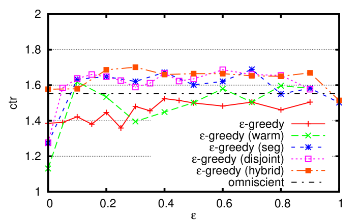
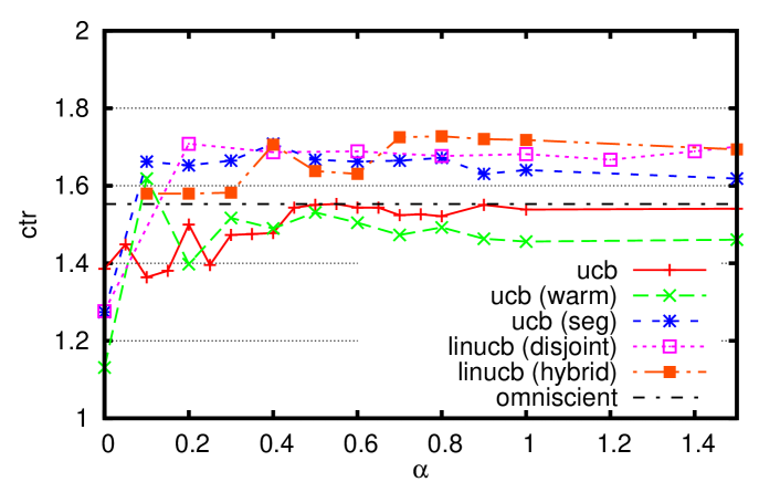
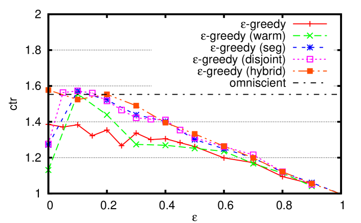
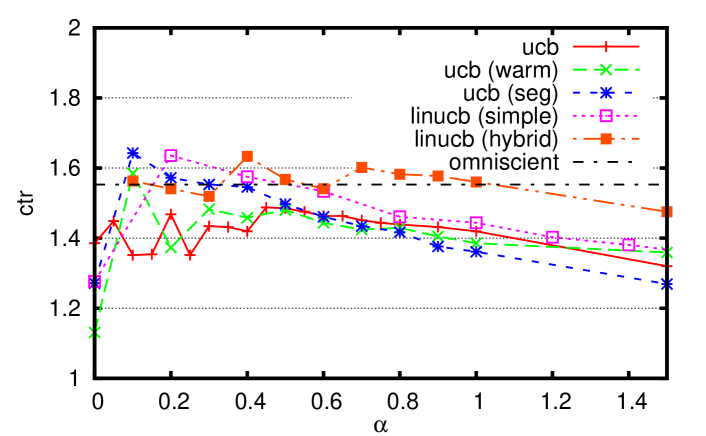
Each of the competing algorithms (except random and omniscient) in Section 5.3 requires a single parameter: for -greedy algorithms and for UCB ones. We used tuning data to optimize these parameters. Figure 2 shows how the CTR of each algorithm changes with respective parameters. All results were obtained by a single run, but given the size of our dataset and the unbiasedness result in Theorem 1, the reported numbers are statistically reliable.
First, as seen from Figure 2, the CTR curves in the learning buckets often possess the inverted U-shape. When the parameter ( or ) is too small, there was insufficient exploration, the algorithms failed to identify good articles, and had a smaller number of clicks. On the other hand, when the parameter is too large, the algorithms appeared to over-explore and thus wasted some of the opportunities to increase the number of clicks. Based on these plots on tuning data, we chose appropriate parameters for each algorithm and ran it once on the evaluation data in the next subsection.
Second, it can be concluded from the plots that warm-start information is indeed helpful for finding a better match between user interest and article content, compared to the no-feature versions of -greedy and UCB. Specifically, both -greedy (warm) and ucb (warm) were able to beat omniscient, the highest CTRs achievable by context-free policies in hindsight. However, performance of the two algorithms using warm-start information is not as stable as algorithms that learn the weights online. Since the offline model for “warm start” was trained with article CTRs estimated on all random traffic [12], -greedy (warm) gets more stable performance in the deployment bucket when is close to . The warm start part also helps ucb (warm) in the learning bucket by selecting more attractive articles to users from scratch, but did not help ucb (warm) in determining the best online for deployment. Since ucb relies on the a confidence interval for exploration, it is hard to correct the initialization bias introduced by “warm start”. In contrast, all online-learning algorithms were able to consistently beat the omniscient policy. Therefore, we did not try the warm-start algorithms on the evaluation data.
Third, -greedy algorithms (on the left of Figure 2) achieved similar CTR as upper confidence bound ones (on the right of Figure 2) in the deployment bucket when appropriate parameters were used. Thus, both types of algorithms appeared to learn comparable policies. However, they seemed to have lower CTR in the learning bucket, which is consistent with the empirical findings of context-free algorithms [2] in real bucket tests.
Finally, to compare algorithms when data are sparse, we repeated the same parameter tuning process for each algorithm with fewer data, at the level of %, %, %, %, and %. Note that we still used all data to evaluate an algorithm’s CTR as done in Algorithm 3, but then only a fraction of available data were randomly chosen to be used by the algorithm to improve its policy.
5.5.2 Results for Evaluation Data
With parameters optimized on the tuning data (c.f., Figure 2), we ran the algorithms on the evaluation data and summarized the CTRs in Table 1. The table also reports the CTR lift compared to the baseline of -greedy. The CTR of omniscient was , and so a significantly larger CTR of an algorithm indicates its effective use of user/article features for personalization. Recall that the reported CTRs were normalized by the random policy’s CTR. We examine the results more closely in the following subsections.
On the Use of Features
We first investigate whether it helps to use features in article recommendation. It is clear from Table 1 that, by considering user features, both -greedy (seg/disjoint/hybrid) and UCB methods (ucb (seg) and linucb (disjoint/hybrid)) were able to achieve a CTR lift of around %, compared to the baseline -greedy.
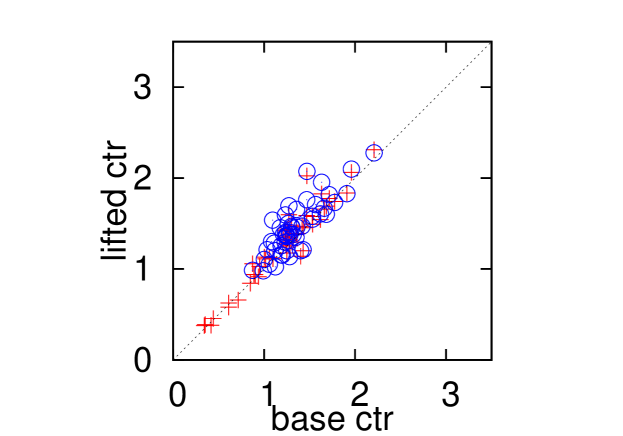
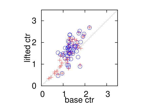
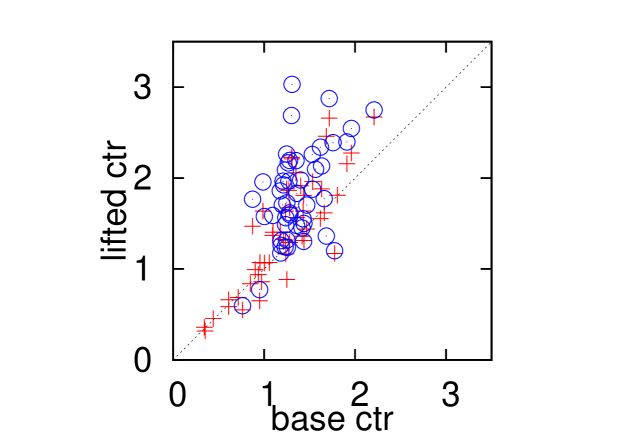
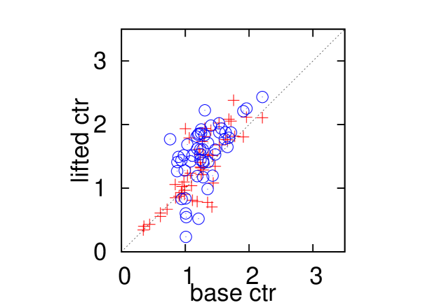
To better visualize the effect of features, Figure 3 shows how an article’s CTR (when chosen by an algorithm) was lifted compared to its base CTR (namely, the context-free CTR).444To avoid inaccurate CTR estimates, only articles that were chosen most often by an algorithm were included in its own plots. Hence, the plots for different algorithms are not comparable. Here, an article’s base CTR measures how interesting it is to a random user, and was estimated from logged events. Therefore, a high ratio of the lifted and base CTRs of an article is a strong indicator that an algorithm does recommend this article to potentially interested users. Figure 3(a) shows neither -greedy nor ucb was able to lift article CTRs, since they made no use of user information. In contrast, all the other three plots show clear benefits by considering personalized recommendation. In an extreme case (Figure 3(c)), one of the article’s CTR was lifted from to —a % improvement.
Furthermore, it is consistent with our previous results on tuning data that, compared to -greedy algorithms, UCB methods achieved higher CTRs in the deployment bucket, and the advantage was even greater in the learning bucket. As mentioned in Section 2.2, -greedy approaches are unguided because they choose articles uniformly at random for exploration. In contrast, exploration in upper confidence bound methods are effectively guided by confidence intervals—a measure of uncertainty in an algorithm’s CTR estimate. Our experimental results imply the effectiveness of upper confidence bound methods and we believe they have similar benefits in many other applications as well.
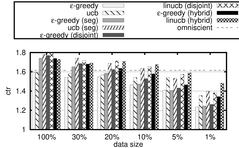
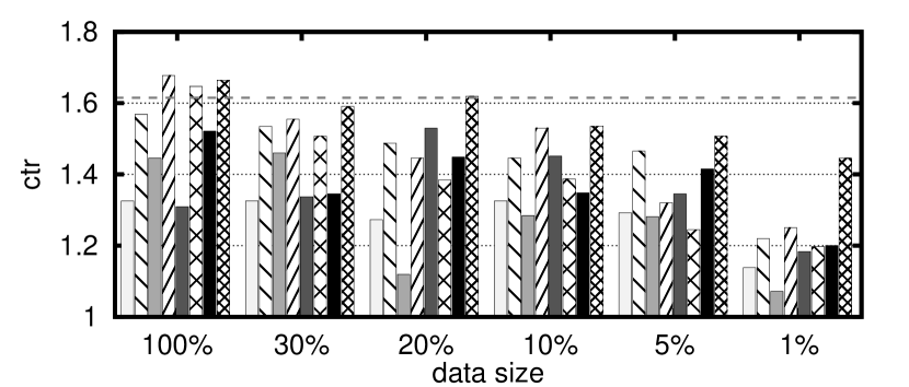
On the Size of Data
One of the challenges in personalized web services is the scale of the applications. In our problem, for example, a small pool of news articles were hand-picked by human editors. But if we wish to allow more choices or use automated article selection methods to determine the article pool, the number of articles can be too large even for the high volume of Yahoo! traffic. Therefore, it becomes critical for an algorithm to quickly identify a good match between user interests and article contents when data are sparse. In our experiments, we artificially reduced data size (to the levels of %, %, %, %, and %, respectively) to mimic the situation where we have a large article pool but a fixed volume of traffic.
To better visualize the comparison results, we use bar graphs in Figure 4 to plot all algorithms’ CTRs with various data sparsity levels. A few observations are in order. First, at all data sparsity levels, features were still useful. At the level of %, for instance, we observed a % improvement of linucb (hybrid)’s CTR in the deployment bucket () over ucb’s ().
Second, UCB methods consistently outperformed -greedy ones in the deployment bucket.555In the less important learning bucket, there were two exceptions for linucb (disjoint). The advantage over -greedy was even more apparent when data size was smaller.
Third, compared to ucb (seg) and linucb (disjoint), linucb (hybrid) showed significant benefits when data size was small. Recall that in hybrid models, some features are shared by all articles, making it possible for CTR information of one article to be “transferred” to others. This advantage is particularly useful when the article pool is large. In contrast, in disjoint models, feedback of one article may not be utilized by other articles; the same is true for ucb (seg). Figure 4(a) shows transfer learning is indeed helpful when data are sparse.
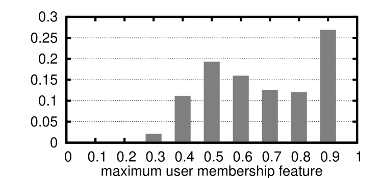
Comparing ucb (seg) and linucb (disjoint)
From Figure 4(a), it can be seen that ucb (seg) and linucb (disjoint) had similar performance. We believe it was no coincidence. Recall that features in our disjoint model are actually normalized membership measures of a user in the five clusters described in Section 5.2.2. Hence, these features may be viewed as a “soft” version of the user assignment process adopted by ucb (seg).
Figure 5 plots the histogram of a user’s relative membership measure to the closest cluster, namely, the largest component of the user’s five, non-constant features. It is clear that most users were quite close to one of the five cluster centers: the maximum membership of about % users were higher than , and about % of them were higher than . Therefore, many of these features have a highly dominating component, making the feature vector similar to the “hard” version of user group assignment.
We believe that adding more features with diverse components, such as those found by principal component analysis, would be necessary to further distinguish linucb (disjoint) from ucb (seg).
6 Conclusions
This paper takes a contextual-bandit approach to personalized web-based services such as news article recommendation. We proposed a simple and reliable method for evaluating bandit algorithms directly from logged events, so that the often problematic simulator-building step could be avoided. Based on real Yahoo! Front Page traffic, we found that upper confidence bound methods generally outperform the simpler yet unguided -greedy methods. Furthermore, our new algorithm LinUCB shows advantages when data are sparse, suggesting its effectiveness to personalized web services when the number of contents in the pool is large.
In the future, we plan to investigate bandit approaches to other similar web-based serviced such as online advertising, and compare our algorithms to related methods such as Banditron [16]. A second direction is to extend the bandit formulation and algorithms in which an “arm” may refer to a complex object rather than an item (like an article). An example is ranking, where an arm corresponds to a permutation of retrieved webpages. Finally, user interests change over time, and so it is interesting to consider temporal information in bandit algorithms.
7 Acknowledgments
We thank Deepak Agarwal, Bee-Chung Chen, Daniel Hsu, and Kishore Papineni for many helpful discussions, István Szita and Tom Walsh for clarifying their algorithm, and Taylor Xi and the anonymous reviewers for suggestions that improved the presentation of the paper.
References
- [1] N. Abe, A. W. Biermann, and P. M. Long. Reinforcement learning with immediate rewards and linear hypotheses. Algorithmica, 37(4):263–293, 2003.
- [2] D. Agarwal, B.-C. Chen, and P. Elango. Explore/exploit schemes for web content optimization. In Proc. of the 9th International Conf. on Data Mining, 2009.
- [3] D. Agarwal, B.-C. Chen, P. Elango, N. Motgi, S.-T. Park, R. Ramakrishnan, S. Roy, and J. Zachariah. Online models for content optimization. In Advances in Neural Information Processing Systems 21, pages 17–24, 2009.
- [4] R. Agrawal. Sample mean based index policies with regret for the multi-armed bandit problem. Advances in Applied Probability, 27(4):1054–1078, 1995.
- [5] A. Anagnostopoulos, A. Z. Broder, E. Gabrilovich, V. Josifovski, and L. Riedel. Just-in-time contextual advertising. In Proc. of the 16th ACM Conf. on Information and Knowledge Management, pages 331–340, 2007.
- [6] P. Auer. Using confidence bounds for exploitation-exploration trade-offs. Journal of Machine Learning Research, 3:397–422, 2002.
- [7] P. Auer, N. Cesa-Bianchi, and P. Fischer. Finite-time analysis of the multiarmed bandit problem. Machine Learning, 47(2–3):235–256, 2002.
- [8] P. Auer, N. Cesa-Bianchi, Y. Freund, and R. E. Schapire. The nonstochastic multiarmed bandit problem. SIAM Journal on Computing, 32(1):48–77, 2002.
- [9] D. A. Berry and B. Fristedt. Bandit Problems: Sequential Allocation of Experiments. Monographs on Statistics and Applied Probability. Chapman and Hall, 1985.
- [10] P. Brusilovsky, A. Kobsa, and W. Nejdl, editors. The Adaptive Web — Methods and Strategies of Web Personalization, volume 4321 of Lecture Notes in Computer Science. Springer Berlin / Heidelberg, 2007.
- [11] R. Burke. Hybrid systems for personalized recommendations. In B. Mobasher and S. S. Anand, editors, Intelligent Techniques for Web Personalization. Springer-Verlag, 2005.
- [12] W. Chu and S.-T. Park. Personalized recommendation on dynamic content using predictive bilinear models. In Proc. of the 18th International Conf. on World Wide Web, pages 691–700, 2009.
- [13] W. Chu, S.-T. Park, T. Beaupre, N. Motgi, A. Phadke, S. Chakraborty, and J. Zachariah. A case study of behavior-driven conjoint analysis on Yahoo!: Front Page Today Module. In Proc. of the 15th ACM SIGKDD International Conf. on Knowledge Discovery and Data Mining, pages 1097–1104, 2009.
- [14] A. Das, M. Datar, A. Garg, and S. Rajaram. Google news personalization: scalable online collaborative filtering. In Proc. of the 16th International World Wide Web Conf., 2007.
- [15] J. Gittins. Bandit processes and dynamic allocation indices. Journal of the Royal Statistical Society. Series B (Methodological), 41:148–177, 1979.
- [16] S. M. Kakade, S. Shalev-Shwartz, and A. Tewari. Efficient bandit algorithms for online multiclass prediction. In Proc. of the 25th International Conf. on Machine Learning, pages 440–447, 2008.
- [17] T. L. Lai and H. Robbins. Asymptotically efficient adaptive allocation rules. Advances in Applied Mathematics, 6(1):4–22, 1985.
- [18] J. Langford and T. Zhang. The epoch-greedy algorithm for contextual multi-armed bandits. In Advances in Neural Information Processing Systems 20, 2008.
- [19] D. J. C. MacKay. Information Theory, Inference, and Learning Algorithms. Cambridge University Press, 2003.
- [20] D. Mladenic. Text-learning and related intelligent agents: A survey. IEEE Intelligent Agents, pages 44–54, 1999.
- [21] S.-T. Park, D. Pennock, O. Madani, N. Good, and D. DeCoste. Naïve filterbots for robust cold-start recommendations. In Proc. of the 12th ACM SIGKDD International Conf. on Knowledge Discovery and Data Mining, pages 699–705, 2006.
- [22] N. G. Pavlidis, D. K. Tasoulis, and D. J. Hand. Simulation studies of multi-armed bandits with covariates. In Proceedings on the 10th International Conf. on Computer Modeling and Simulation, pages 493–498, 2008.
- [23] D. Precup, R. S. Sutton, and S. P. Singh. Eligibility traces for off-policy policy evaluation. In Proc. of the 17th Interational Conf. on Machine Learning, pages 759–766, 2000.
- [24] H. Robbins. Some aspects of the sequential design of experiments. Bulletin of the American Mathematical Society, 58(5):527–535, 1952.
- [25] J. B. Schafer, J. Konstan, and J. Riedi. Recommender systems in e-commerce. In Proc. of the 1st ACM Conf. on Electronic Commerce, 1999.
- [26] W. R. Thompson. On the likelihood that one unknown probability exceeds another in view of the evidence of two samples. Biometrika, 25(3–4):285–294, 1933.
- [27] T. J. Walsh, I. Szita, C. Diuk, and M. L. Littman. Exploring compact reinforcement-learning representations with linear regression. In Proc. of the 25th Conf. on Uncertainty in Artificial Intelligence, 2009.