UCRL-JRNL-423904 Reaction rate sensitivity of ⁴⁴Ti production in massive stars and implications of a thick target yield measurement of ⁴⁰Ca($\alpha$,$\gamma$)⁴⁴Ti

Abstract

We evaluate two dominant nuclear reaction rates and their uncertainties that affect ⁴⁴Ti production in explosive nucleosynthesis. Experimentally we develop thick-target yields for the ⁴⁰Ca($\alpha$,$\gamma$)⁴⁴Ti reaction at $E_{\rm\alpha}=4.13,4.54$, and $5.36$ MeV using $\gamma$-ray spectroscopy. At the highest beam energy, we also performed an activation measurement which agrees with the thick target result. From the measured yields a stellar reaction rate was developed that is smaller than current statistical-model calculations and recent experimental results, which would suggest lower ⁴⁴Ti production in scenarios for the $\alpha-$rich freeze out. Special attention has been paid to assessing realistic uncertainties of stellar reaction rates produced from a combination of experimental and theoretical cross sections. With such methods, we also develop a re-evaluation of the ⁴⁴Ti($\alpha$,$p$)⁴⁷V reaction rate. Using these two rates we carry out a sensitivity survey of ⁴⁴Ti synthesis in eight expansions representing peak temperature and density conditions drawn from a suite of recent supernova explosion models. Our results suggest that the current uncertainty in these two reaction rates could lead to as large an uncertainty in ⁴⁴Ti synthesis as that produced by different treatments of stellar physics.

1 INTRODUCTION

The dynamic synergy between observation, theory, and experiment developed over many years around the field of $\gamma$-ray astronomy has as its ultimate goal observations of specifc radionuclides informing our understanding of stellar explosions and the theoretical models that predict nucleosynthesis. Of the radioactive species observed so far, the most long lived, ²⁶Al and ⁶⁰Fe (with half-lives $\tau_{1/2}=7.17\pm 0.24\times 10^{5}$ and $2.62\pm 0.04\times 10^{6}$ yr, respectively), are in reasonably good agreement with theoretical predictions (Timmes et al., 1996; Diehl et al., 2006). Observations of those in the iron group, ^56,57Ni ($\tau_{1/2}=6.075\pm 0.01$ d and $35.6\pm 0.06$ hr, respectively) and their decay products ^56,57Co ($\tau_{1/2}=77.233\pm 0.027$ d and $271.74\pm 0.06$d, respectively), are used in many ways to constrain our current models of the core collapse explosion mechanism. The radionuclide ⁴⁴Ti ($\tau_{1/2}=58.9\pm 0.3$ yr), made in the same explosive environment but in much lower amounts compared to the very abundant nickle isotopes (Woosley et al., 1973, 1995), is hoped to one day serve as an even more sensitive diagnostic and a valuable probe of the conditions extant in some of the deepest layers to be ejected.

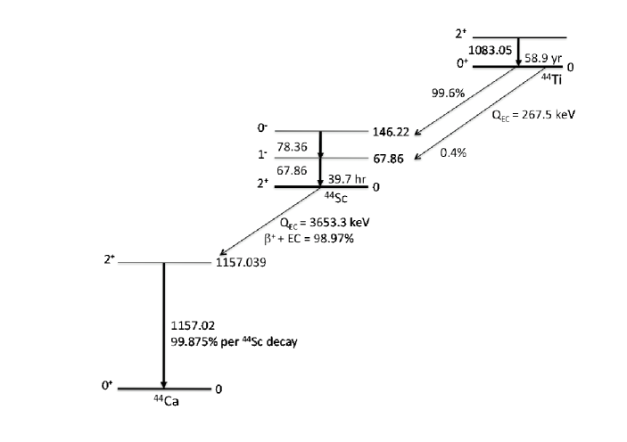
Figure 1: Partial decay schemes of ⁴⁴Ti and its daughter ⁴⁴Sc.

Observationally most of the attention has focused on the detection of the 68, 78, and 1157 keV $\gamma$-rays from the ⁴⁴Ti $\rightarrow$ ⁴⁴Sc $\rightarrow$ ⁴⁴Ca decay chain (see Figure 1). The 1157 keV $\gamma$-ray has been observed directly from a point source in Cassiopeia A (Cas A; Iyudin et al. 1994). This was later confirmed by observation of the low-energy ⁴⁴Sc $\gamma$-rays using the BeppoSax (Vink et al., 2001) and INTEGRAL (Renaud et al., 2006) observatories. Using values for the distance, age, and $\gamma$-flux of Cas A, the amount of ⁴⁴Ti ejected was found to be 1.6${}^{+0.6}_{-0.3}$ $\times$10^-4 M_⊙ (Renaud et al., 2006), in agreement with earlier observations using CGRO (Timmes et al., 1996). Although the presence of ⁴⁴Ti is currently below detection limits in SN1987A in the nearby Large Magellanic Cloud, its light curve is theorized to now be powered by the decay of ⁴⁴Ti. The yield of ⁴⁴Ti in SN1987A has been estimated from its light curve to be $1-2\times 10^{-4}M_{\odot}$, a factor of 3 greater than predicted by models (Diehl et al., 2006). A third ⁴⁴Ti source (of lower significance compared to the one in CasA) has been observed in the Vela region (Iyudin et al., 1998) but the existence of a co-located young supernova (SN) remnant has not been confirmed. While the mass of ⁴⁴Ti observed in SN remnants appears to be underproduced by past models, the number of observed sources of ⁴⁴Ti in all-sky surveys appears to be less than expected from estimates of the Galactic SN rate and the known ⁴⁴Ti half life, leading some to question whether ⁴⁴Ti-producing SNe are exceptional (The et al., 2006).

Theoretically, ⁴⁴Ti production is traditionally ascribed to regions experiencing a strong ”$\alpha-$rich freeze out”, where material initially in nuclear statistical equilibrium (NSE) at relatively low density is cooled so rapidly that free $\alpha-$particles do not have time to reassemble, through inefficient $3-$body reactions that span the mass gaps at A=5 and A=8, back into the iron group. A likely scenario is material in or near the silicon shell as it experiences shock wave passage during a core collapse SN event. Assuming the material cools adiabatically over a hydrodynamic timescale ($\tau_{\rm HD}=446\chi/\sqrt{\rho_{i}}$), where $\chi$ is a scaling parameter (here unity) and $\rho_{i}$ is the initial (peak) density in g cm^-3, initial conditions that would result in a final $\alpha$-particle mass fraction of $\sim$ 1% would require temperatures high enough to ensure NSE ($T_{9i}\gtrapprox 5$) and an initial density $\rho_{i}<{\rm min}(4.5\times 10^{5}T_{9i}^{3},\quad 2.5\times 10^{5}T_{9i}^{4}\chi^{-2/3})$ (Woosley et al., 1973). This translates to a radiation entropy greater than unity (Section 3.2).

In models of massive stars the $\alpha-$rich freeze out dominates the solar production of several species, including ⁴⁴Ca (made as Ti), ⁴⁵Sc, ⁵⁷Fe (made as Ni), and ^58,60Ni, while still others seem to require a sizable component to account for their solar abundances, including ^50,52Cr, ⁵⁹Co, ⁶²Ni, and ⁶⁴Zn (Woosley et al., 1995; Thielemann, Nomoto, & Hashimoto, 1996). Although ⁵⁶Ni is the dominant species produced in both NSE and the $\alpha-$rich freez out over a wide range ($0\leq\eta\leq 0.01$) of neutron excess (Hartmann, Woosley, & El Eid, 1985), the solar abundance of ⁵⁶Fe is dominated by production in explosive silicon burning in massive stars and by a large contribution from SNe Ia (Timmes, Woosley, & Weaver, 1995).

In order to address one aspect of the model uncertainties associated with the theoretical predictions of ⁴⁴Ti in SNe, we focus on exploring the nuclear data uncertainties of two key reaction rates. Experimentally we address the ⁴⁰Ca($\alpha$,$\gamma$)⁴⁴Ti cross section where the existing experimental results are inconsistent and theoretical estimates are complicated by the suppression of $E1$ $T=0\rightarrow T=0$ gamma transitions in self-conjugate ($N$ = $Z$) nuclei (Rauscher et al., 2000). This cross section has been measured in the past using several techniques. Cooperman et al. (1977) used in-beam $\gamma$-ray spectroscopy to measure the capture of $\alpha$-particles on a metallic calcium target in the center-of-mass energy range $E_{\rm CM}=2.5-3.65$ MeV. In that work the excitation function for the 1083 keV first excited state transition in ⁴⁴Ti was determined and the resonance strengths were developed. Nassar et al. (2006) determined the integral cross section in the range $E_{\rm CM}=2.2-4.17$ MeV by bombarding a He gas target with a ⁴⁰Ca beam and collecting the recoiling ⁴⁴Ti in a catcher foil. Accelerator mass spectroscopy was then used to determine the ratio of ⁴⁴Ti/Ti from the known content of Ti in the catcher foil. Recently, a slightly broader energy range of $E_{\rm CM}=2.11-4.19$ MeV was explored using the DRAGON recoil mass spectrometer (Vockenhuber et al., 2007) in inverse kinematics. They developed individual resonances whose sum was used to determine a reaction rate for $1\leq T_{9}\leq 5.5$. Yet despite these often heroic expenditures of time, toil, and treasure, in the temperature range of astrophysical interest there still exists a factor of 3 or more difference between the experimentally determined reaction rates.

In this work, we develop the cross section for ⁴⁰Ca($\alpha$,$\gamma$)⁴⁴Ti by two separate methods as a check on systematic uncertainties. First we used in-beam $\gamma$-ray spectroscopy to measure a thick target yield of the ⁴⁰Ca($\alpha$,$\gamma$)⁴⁴Ti reaction. We then determined the number of ⁴⁴Ti nuclei produced by counting low-energy $\gamma$-rays from the decay of ⁴⁴Ti in an irradiated target. Special attention was devoted to checking the internal consistency of the measurements and to establishing realistic uncertainties in developing the stellar reaction rate from a combination of experimental and theoretical cross sections. We have made a similar evaluation of the stellar reaction rate for the dominant destruction reaction, ⁴⁴Ti($\alpha$,$p$)⁴⁷V, based on the original experimental work of Sonzogni et al. (2000) and the theoretical cross section work of Rauscher & Thielemann (2001).

Our results are presented in four parts. In Section 2, we describe our experimental efforts. Section 3 then discusses the development of stellar reaction rates, and an expose of the past and present experimental and theory efforts for the two rates in question. In Section 4, we present nucleosynthesis results for the production of ⁴⁴Ti and ^56,57,58Ni reported in previous surveys of massive star evolution. We then carry out a sensitivity survey of ⁴⁴Ti to variations in the principle production and destruction rates using more recent SN models. In Section 5 we provide a discussion and conclusions.

2 Experimental Methods

The ⁴⁰Ca($\alpha$,$\gamma$)⁴⁴Ti reaction was measured at the Lawrence Livermore National Laboratory (LLNL) Center for Accelerator Mass Spectroscopy (CAMS) using a 10 MV FN Tandem Van de Graaff accelerator. To calibrate the beam energy a silicon detector was placed in a low current beam and the measured energy was then compared with spectroscopy grade $\alpha$-sources. The $\alpha$ energies used were the 5.30 MeV from ²¹⁰Po, the 6.12 MeV from ²⁵²Cf, the 5.49 MeV from ²⁴¹Am, and the 4.69 and 4.61 MeV $\alpha$’s from the decay of ²³⁰Th. From the calibration, the uncertainty in the $\alpha$-beam energy is $\pm$ 5 keV. The thick target yield was measured at $E_{\rm\alpha}=4.13$, $4.54$, and $5.36$ MeV beam energies.

For each beam energy a target was manufactured by pressing ^natCaO powder into a copper holder. The powder had a purity of 99.95$\%$ (metals basis) but contained ppm concentrations of C and F. To completely stop the beam, each target had a minimum thickness of at least 1.1 mm. The target was mounted on a copper block within the vacuum chamber and tilted at 30^∘ with respect to the beam. The vacuum chamber contained two windows so that the target could be visually monitored. A schematic of the target chamber is given in Figure 2.

The target chamber was electrically isolated from the rest of the beam line. The target was electrically connected to the target chamber allowing the beam current to be directly measured from the chamber. The current integration from the target chamber was checked to a precision of better than 1$\%$ using a NIST-traceable precision DC current source. An opposing-pair magnet was attached upstream of the target chamber to suppress the escape of secondary electrons generated by the beam on the target. A summary of the irradiation runs is given in Table 1.

Table 1: Irradiation Conditions for the ^natCaO Targets.

Irradiation Run	$E_{\alpha}$ (MeV)	Irradiation Time (hr)	Total Charge ($\mu$C   )
1	4.13	6	45808.6
2	4.54	7	46115.8
3	5.36	10	25763.2

Two 80$\%$ HPGe detectors were used to measure the prompt $\gamma$-ray yield during irradiation. One detector was 11.4 cm away from the target at 30^∘ with respect to the beam. The location of the second detector was at 15.8 cm and an angle of 99^∘. The HPGe detector thresholds were set at 125 keV. The average deadtime during a run was 10 %.

The $\gamma$-ray energy spectra was accumulated in 8192 channels using two Ortec AD413a ADCs. Efficiency and energy calibrations of the HPGe detectors were made using ⁶⁰Co, ²²Na, ¹³⁷Cs, ⁵⁴Mn, and ¹³³Ba NIST-traceable sources with activities known to a $1\sigma$ uncertainty of 1$\%$. Efficiencies of 0.085$\%$ and 0.162$\%$ were found for the detectors at 30^∘ and 99^∘, respectively.

2.1 Analysis of Prompt $\gamma$-Ray Data

The thick target yield for the ⁴⁰Ca($\alpha$,$\gamma$)⁴⁴Ti reaction was deduced from the yield of the 2⁺$\rightarrow$0⁺ 1083 keV transition which collects most of the strength from ⁴⁴Ti. The angular distribution of the 1083 keV $\gamma$-rays with respect to the angle between the $\gamma$-rays and beam direction is given by $W(\theta)=\sum_{l}a_{l}P_{l}(\cos\theta)$ with $l$ = 0, 2, 4. The cross section is proportional to $a_{0}$ so only this term needs to be determined (Dyer et al., 1981). By placing the detectors at angles for which $P$₄($\cos\theta$) is zero, 30.6^∘ and 109.9^∘, $a_{0}$ can be determined from measurements at only two angles. The experimental thick target yield of the 1083 keV $\gamma$-ray at angle $\theta$ is given by

$$Y_{1083}(\theta)=\frac{N_{c}}{N_{p}L_{t}A_{b}\,\varepsilon_{1083}},\$$ (1)

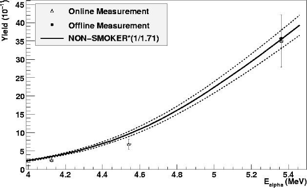
Figure 4: Measured thick target yields compared to the calculated NON-SMOKER thick target yield. The online measurement is the measured yield for the 1083 keV $\gamma$-ray corrected upward by 20$\%$ (see the text). The $E_{\alpha}$ = 5.36 MeV offline counting data point and its error is plotted as measured. The NON-SMOKER cross section required a downward scaling of 1.71 to match the off-line data point. The dashed lines indicate the normalization needed to match the offline error bars.

where $N_{c}$ is the number of counts in the 1083 keV photopeak, $N_{p}$ is the number of $\alpha$ particles impinging on the target, $L_{t}$ is the detector live-time fraction, $A_{b}$ is the natural abundance of ⁴⁰Ca, and $\varepsilon_{1083}$ is the efficiency of the HPGe detector at 1083 keV. The region near the 1083 keV $\gamma$-ray is shown in Figure 3 for $E_{\alpha}$ = 5.36 MeV. The 1083 keV photopeak lies on the tail of the 1039 keV ⁷⁰Ge doppler shifted $\gamma$-ray excited by fast neutrons primarily from the ¹⁹F($\alpha,n$) reaction. The background and 1083 keV peak were fit to an error function convoluted with a Gaussian, as in Gete et al. (1997). The total experimental yield for the 1083 keV $\gamma$-ray was determined by finding $a_{0}$ from the angular distribution of $Y(\theta)$. The experimental yield of the 1083 keV $\gamma$-ray determined from these fits are given in Table  2. In order to convert the yield of the 1083 keV $\gamma$-ray into the yield of ⁴⁴Ti, one must take into account those transitions which bypass the 2${}^{+}\rightarrow$ 0⁺ 1083 keV transition in ⁴⁴Ti. The Monte Carlo program DICEBOX (Becvar, 1998) was used to simulate the $\gamma$-ray cascades from the decay of the compound nucleus ⁴⁴Ti in order to estimate the number of transitions which bypass the 2${}^{+}\rightarrow$ 0⁺ transition. These simulations suggest $(20\pm 3)$% of transitions bypass the 2${}^{+}\rightarrow$ 0⁺ transition with the error on the simulations taking into account the uncertainty in the nuclear level density, the photon strength function, and the capture state. In Figure 4, the thick target yield corrected for the missed strength to the 1083 keV level is compared to the NON-SMOKER cross section.

Table 2: ⁴⁰Ca($\alpha$,$\gamma$)⁴⁴Ti Measured and Theoretical Thick Target Yields per $\alpha$ Particle on Target. $Y_{1083}$ is the measured yield for the 1083 keV $\gamma$-ray, $Y_{{}^{44}\rm Ti}$ is the total yield for the production of ⁴⁴Ti, and $Y_{\rm theory}$ the thick target yield calculated from Equation 2 assuming the theory cross section of Rauscher & Thielemann (2001). $Y_{\rm offline}$ is the yield from our activation measurement of the target irradiated at 5.36 MeV.

$E_{\alpha}$ (MeV)	$Y_{1083}$ (10-11)	$Y_{{}^{44}\rm Ti}$ (10-11)	$Y_{\rm theory}$ (10-11)	$Y_{\rm offline}$ (10-11)
4.13	2.11 $\pm$ 0.40	2.53 $\pm$ 0.50	5.96
4.54	5.72 $\pm$ 1.1	6.86 $\pm$ 1.4	16.4
5.36	29.2 $\pm$ 5.7	35.0$\pm$ 7.1	61.0	35.7 $\pm$ 2.5

The experimental yield can be related to a theoretical cross section $\sigma(E)$ by the equation

$$Y=\int^{E_{\alpha}}_{0}\frac{\sigma(E)}{-dE/dx}dE$$ (2)

where $\sigma$($E$) is the energy-dependent cross section, and $dE/dx$ is the stopping power for ^natCaO. The $dE/dx$ values for ^natCaO were calculated using the program SRIM (J.F. Ziegler, 2004). Table  2 gives a comparison of the experimental and calculated yields using the NON-SMOKER Hauser-Feshbach ⁴⁰Ca($\alpha$,$\gamma$)⁴⁴Ti cross section (Rauscher & Thielemann, 2001). The experimental yields are a factor of 1.7-2.3 times smaller than the yield calculated from the theoretical cross sections.

The uncertainties from detector efficiencies, deadtime, angular distribution corrections, coincidence summing, and beam current integration are tabulated in Table 3. The integrated beam current was cross checked by using the ¹⁷O($\alpha,\alpha^{\prime}\gamma$) and ⁴⁴Ca($\alpha,\alpha^{\prime}\gamma$) reactions. The thick target yield for the ¹⁷O($\alpha,\alpha^{\prime}\gamma$) reaction that excites the first excited state at 870.8 keV was measured in Hsu (1982) at $E_{\alpha}$ = 5.486 MeV. Using Equation (1), $N_{p}$ from ¹⁷O($\alpha,\alpha^{\prime}\gamma$) was determined to be (7.2$\pm$0.86$)\times$10¹⁶ after correcting for the difference in beam energy between Hsu (1982) and our work. The thick target yield for the Coulomb excitation of the 1157 keV level in ⁴⁴Ca was calculated using the program GOSIA (Czosnyka et al., 1983) and used to infer $N_{p}$ of (8.2$\pm$1.6)$\times$10¹⁶. This compares well with our beam current integrator which gave a value of 7.2$\times$10¹⁶ for $N_{p}$. The efficiency of the detector at 30^∘ was sensitive to the decay location due to the attenuation of $\gamma$-rays through the copper target holder. By varying the position of $\gamma$-ray sources to match the approximate 1 cm² beam spot size the uncertainty in the efficiency was determined. The uncertainty due to coincidence summing of $\gamma$-rays in a single detector was estimated from the geometric solid angle spanned by the detectors.

Table 3: Compilation of systematic uncertainties for the online measurement (1$\sigma$).

Source of uncertainty	Uncertainty
Beam integration	1%
Detector efficiency	6%-7%
Deadtime	1%
Angular distribution	17%-18%
Coincidence summing	1%

The angular distribution is the largest source of uncertainty. Our detectors did not sit at exactly the zeros of the $P_{4}$ term in the angular distribution which introduces some uncertainty when $a_{0}$ is determined with only two detectors. Furthermore, Simpson et al. (1971) measured the angular distribution of $\gamma$-rays following resonance $\alpha$ capture at $E_{\alpha}$ = 4.22, 4.26, and 4.52 MeV and found a strong contribution for the $P_{4}$ term. The uncertainty on $a_{0}$ was estimated by the following procedure. A value was chosen for the $a_{4}$ coefficient between $\pm$0.5 and then a fit of the angular $\gamma$-ray yield was made. The resulting variation in $a_{0}$ was between 17% and 18% for different values of $a_{4}$. This is a conservative estimate because the many $\gamma$-ray cascade paths and alpha energies involved are likely to wash out any nuclear alignment and would cause $a_{4}$ to be nearly zero.

2.2 Low Background Counting

The offline counting of the irradiated target took place at the Low Background Counting facility at LLNL. Only the target irradiated at $E_{\alpha}$ = 5.36 MeV was counted because the activity of the other targets was estimated to be too low. A HPGe low-energy photon spectrometer (LEPS) detector was used to detect 68 and 78 keV $\gamma$-rays from ⁴⁴Ti decay. The target was placed 2 mm away from the detector face and counted for two weeks. The activity of the ⁴⁴Ti target was determined by comparing it to a 56.6 $\pm$ 1.6 nCi ⁴⁴Ti reference source. The reference source was counted with the LEPS detector in the same geometry as the ⁴⁴Ti target.

The ⁴⁴Ti reference source strength was determined by using an 80$\%$ HPGe detector to compare the 1157 keV $\gamma$-ray to a ²²Na and ⁶⁰Co calibrated source. The count was made at a distance of 60 cm away from the detector in order to avoid summing of the 1157 keV $\gamma$-ray with the 511 keV $\gamma$-ray.

The yield was found from

$$Y=\frac{A\,T_{\frac{1}{2}}}{N_{p}\ln 2},$$ (3)

where $A$ is the activity of the irradiated target and $\tau_{1/2}=58.9\pm 0.3$ years is the ⁴⁴Ti half-life (Ahmad et al., 2006).

A simultaneous fit of the peaks in Figure 5 gives an experimental yield of (35.7 $\pm$ 2.5) $\times$ 10^{-11 44}Ti per $\alpha$-particle. The uncertainty in the offline yield takes into account the uncertainty in the detector efficiency, half-life, integration of beam current, calibration source strength, and statistics. Since the activity of the ⁴⁴Ti target was determined with a reference source having the same decay scheme the need to correct for summing of the 68 and 78 keV $\gamma$-rays was eliminated. This yield is 22$\%$ higher than the yield from the online counting and agrees with the estimate that (20$\pm$3)$\%$ of $\gamma$-ray cascades bypass the 1083 keV level. This also demonstrates that sputtering of the target was minimal during particle bombardment.

3 Reaction Rates

3.1 The True Gamow Window

Thermonuclear reaction rates are obtained through integration of the energy-dependent cross section weighted by a Maxwell-Boltzmann (MB) particle distribution (Fowler, Caughlan & Zimmerman, 1967). For reaction $I^{\mu}(j,k)L^{\nu}$

$$N_{A}\langle{\bar{\sigma}_{jk}^{\mu}}v\rangle={{3.732\times 10^{10}}\over{{\hat{A}_{j}}^{1/2}{T_{9}}^{3/2}}}\int_{0}^{\infty}{\bar{\sigma}_{jk}^{\mu}}E_{j}^{\mu}\exp(-11.605E_{j}^{\mu}/T_{9})dE_{j}^{\mu}$$ (4)

where $N_{A}$ is Avagadro’s number, ${\hat{A}_{j}}\sim 3.64$ is the reduced mass of the target and incident projectile in atomic mass units, $\mu$ is an index representing bound states in the target and product nuclei ($\mu=0$ for the ground state, 1 for first excited, etc.), and $v$ is the relative velocity of the $\alpha$-particle ($j$) and the target ($I^{\mu}$) in cm s^-1. The cross section ${\bar{\sigma}_{jk}^{\mu}}$ is expressed in barns, $E_{j}^{\mu}$ is the center of mass energy of the $\alpha$-particle and the target in MeV, $T_{9}$ is the temperature in billions of degrees Kelvin, and the reaction rate has units of cm³ mole^-1 s^-1.

There are two important issues regarding the cross section ${\bar{\sigma}_{jk}^{\mu}}$ used in the integration and its relation to the experimental cross section. First, when computing astrophysically relevant reaction rates, the cross section has to be the one for a thermally excited target nucleus in the plasma. Only such a stellar cross section allows application of detailed balance to derive the reverse rate (Holmes et al., 1976; Rauscher et al., 2009). Laboratory cross sections are measured with the target nucleus in the ground state only and the correction, or stellar enhancement factor, has to be calculated from theory. For the ⁴⁰Ca($\alpha,\gamma$)⁴⁴Ti and ⁴⁴Ti($\alpha,p$)⁴⁷V reactions the correction factors are unity over the entire temperature range of interest (Rauscher & Thielemann, 2000). Therefore the cross section ${\bar{\sigma}_{jk}^{\mu}}$ is identical to the cross section $\sigma$ appearing in Eq. 2.

Second, the question arises as to how well the reaction rate is constrained by the experimental cross section data. In the rare case of a thick target yield measurement that completely samples the relevant stellar temperature range, a direct calculation of the thermonuclear reaction rate can be obtained by introducing a simple change of variable and combining Eq.’s 2 and 4 (Roughton et al., 1976). More often limitations of the experimental apparatus and/or beam time allotment restricts the measurement of cross section data to a fairly narrow energy range. To produce a reaction rate spanning a realistic temperature range for stellar synthesis, one often has to supplement the experimental results with theory cross section values to perform the integration in Eq. 4. The integrand exhibits a maximum contributing most to the reaction rate due to the folding of the energy-dependences of the cross section and the MB distribution. Conventionally, the location and width of this Gamow peak are estimated by multiplying a Coulomb barrier penetration factor with the high-energy tail of the MB distribution or by considering a Gaussian approximation to it (see, e.g., Clayton (1984); Rauscher (2010)).

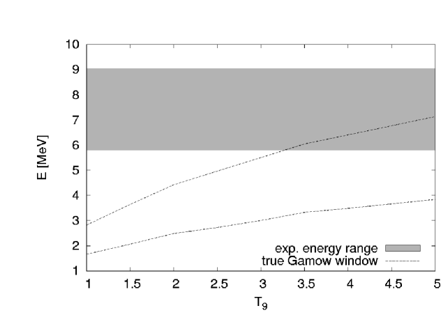
Figure 8: Same as Figure 7 but for the ⁴⁴Ti($\alpha$,$p$)⁴⁷V reaction.

However, this is applicable for capture reactions only as long as the $\gamma$-width is larger than the charged particle width (Iliadis, 2007). Since the $\alpha$ width is changing rapidly with energy due to the Coulomb barrier, this prerequisite may only be fulfilled at very low projectile energies which effectively shifts the Gamow window to lower energies than expected from the standard approximation formula. Figure 6 confirms this by showing the “true” Gamow window at $T_{9}=2$ and $T_{9}=5$ in comparison to the peaks obtained from the standard formula and its approximation for the ⁴⁰Ca($\alpha,\gamma$)⁴⁴Ti and ⁴⁴Ti($\alpha,p$)⁴⁷V reactions. Finally, Fig. 7 compares the energy range spanned by our experimental data with the true Gamow window for stellar temperatures $1\leq T_{9}\leq 5$. The width of the window is defined such that filling the ”window” with experimental data would determine the reaction rate to 10% accuracy. The minimum temperature at which an experiment can fully inform the reaction rate is the overlap of the full width of the window and the range of experimental data (shaded region). For the astrophysical processes considered here, the most relevant temperature range is between $2.0\leq{\rm T}_{9}\leq 4.0$ (Section 3.4). A less severe situation exists for the ⁴⁴Ti($\alpha,p$)⁴⁷V (Figure 8). From these figures it is evident that the limited range of experimental data collected in these two experiments do not contribute significantly to the rates in the important temperature range and that the supplemental theory cross sections at lower energies will dominate both of the rates and their uncertainties. Nevertheless, the data can be used to test the NON-SMOKER predictions at higher energies.

3.2 Reaction Rate for ⁴⁰Ca($\alpha,\gamma$)⁴⁴Ti

To obtain a “semi-experimental” astrophysical rate for ⁴⁰Ca($\alpha,\gamma$)⁴⁴Ti, we normalized the NON-SMOKER cross section by a factor of 1.71 to agree with our measured thick target yield at 5.36 MeV (Figure 4). The data at this energy were chosen because the experimental result was confirmed by two independent techniques. Although the errors on the experimental thick target yield are small, during the calcuation of the reaction rate we have to assign an uncertainty which is similar to the uncertainty on the theory cross section. Therefore we will perform our astrophysical studies with an assigned factor of 2 uncertainty on this rate. This also accounts for a potentially different energy-dependence of the theoretical cross section, and fits well with the general factor of $2-3$ accuracy expected for global predictions of low-energy $\alpha$-capture reactions on self-conjugate nuclei (Rauscher et al., 2000).

The resulting reaction rates were then fit assuming the REACLIB parameterization (Rauscher & Thielemann, 2001).

$$N_{A}<\sigma\nu>=\exp(a_{0}+a_{1}{T_{9}}^{-1}+a_{2}{T_{9}}^{-1/3}+a_{3}{T_{9}}^{1/3}+a_{4}{T_{9}}+a_{5}{T_{9}}^{5/3}+a_{6}\ln({T_{9}}))$$ (5)

where $T_{9}$ is the temperature in $10^{9}$ K. The fit is defined in the range $0.01\leq{\rm T}_{9}\leq 10.0$. The reverse rate for ⁴⁴Ti($\gamma,\alpha$)⁴⁰Ca is calculated through detailed balance, the $Q$ value of the forward reaction is 5.1271 MeV.

Figure 9 shows the ⁴⁰Ca($\alpha,\gamma$)⁴⁴Ti reaction rates considered in this study. The values are generated from fits to reaction rates developed from numerous experimental and theory efforts carried out over the last 20 years. Some have been used in widely cited nucleosynthesis surveys. In particular, Woosley et al. (1995) utilized the theory rates from Woosley et al. (1978), while Limongi & Chieffi (2006) used the fit published in Rauscher & Thielemann (2000). Rauscher et al. (2002) used this same fit but normalized at $T_{9}=3$ to the ”empirical” rate developed in Rauscher et al. (2000). Only ”experimentally” determined rates are shown in the main panel, along with the tabulated Hauser-Feshbach theory based rate (crosses) of Rauscher & Thielemann (2001), hereafter referred to as NON-SMOKER. Also plotted in the inset is the ratio of each rate versus the NON-SMOKER rate, our recommended ⁴⁰Ca($\alpha,\gamma$)⁴⁴Ti rate lies between the oldest and most recent experimental results.

For ⁴⁴Ti synthesis the most relevant temperature range is $2.0\leq{\rm T}_{9}\leq 4.0$. Over this range experimental ⁴⁰Ca($\alpha$,$\gamma$)⁴⁴Ti rates vary by factors of 3-5, respectively. The two most recent experimental rates (Nassar et al., 2006; Vockenhuber et al., 2007) are larger than our recommended rate and would suggest increased ⁴⁴Ti synthesis over our result and the yet smaller original experimental result of Cooperman et al. (1977).

The range of variation in the theory rates is also large, that of Woosley et al. (1978) being of the order of the largest experimental results, the smallest is clearly that of Rauscher & Thielemann (2000). Most unfortunately, the rate generated from this published fit differs from the tabulated NON-SMOKER rate (crosses) by factors of 2 (high and low) on both ends of the important temperature range. Rauscher & Thielemann (2000) fit this rate to an accuracy of 0.92 over the temperature range $0.1\leq T_{9}\leq 10$. In general fits to charged particle rates have larger deviations than those for neutron-induced reactions. Most often a quote of low accuracy pertains to deviation at the lowest temperature points of the fit. Based on arguments related to the nuclear level density and its impact on the applicability of the statistical model, Rauscher & Thielemann (2000) suggest that the lower limit of applicability for this dominant production rate is $T_{9}=0.24$, well below the important temperature range in this study. To be fair the statistical result itself could well be in error by a factor of 2 or more due to the uncertainty in the global $\alpha+$nucleus optical potential, and the fit does agree at $T_{9}=2.8$, which is close to the midway point of ⁴⁴Ti production in several of the scenarios studied in the next section. We have re-fit this rate (dotted line in the inset), and observe that over the important temperature range it now differs from the NON-SMOKER rate by no more that 12% (typically better than 5%). We will include both fits in our sensitivity analysis.

With an uncertainty of a factor of 2, our new ”semi-experimental” rate encompasses most of the previous experiments and calculations. This underlines the necessity for further measurements in the relevant astrophysical energy range (2-5 MeV).

3.3 Reaction Rate for ⁴⁴Ti($\alpha,p$)⁴⁷V

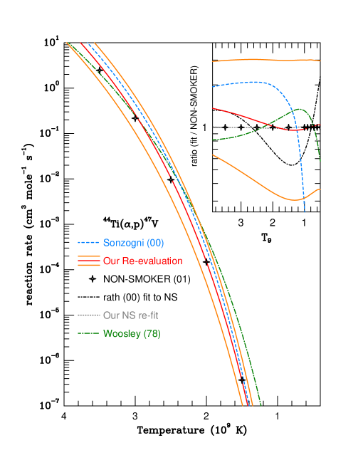
Figure 10: Fits to reaction rates for ⁴⁴Ti($\alpha$,$p$)⁴⁷V considered in this study. Solid line type denotes our re-evaluation and its likely error ($\pm\times 3$) of the lone experimental rate (dashed-line type) of Sonzogni et al. (2000), while the tabulated NON-SMOKER theory rate (Rauscher & Thielemann, 2001) is denoted by crosses. The inset illustrates the ratio of each reaction rate to the NON-SMOKER rate, including the (dot-short-dash) original fit (Rauscher & Thielemann, 2000), our attempt (dotted) to refit the tabulated NON-SMOKER rate, and the theory rate (dot-long-dash) from Woosley et al. (1978).

Figure  10 shows a similar comparison for the ⁴⁴Ti($\alpha,p$)⁴⁷V rates. As with the dominant production rate, the original Rauscher & Thielemann (2000) fit to this destruction rate is in poor agreement with the statistical NON-SMOKER rate (crosses). They list a fit uncertainty of 0.12 and the lower limit of applicability as $T_{9}=0.035$, again outside the important temperature range in this study. We also note that the NON-SMOKER rate exceeds the older (dot-long-dash line) statistical result of Woosley et al. (1978) for $T_{9}\geq 2.4$, which would suggest decreased ⁴⁴Ti production over that seen in the survey of Woosley et al. (1995).

The only published experimental reaction rate (Sonzogni et al., 2000) is roughly a factor of 2 above the NON-SMOKER rate, which would suggest even further decreased ⁴⁴Ti synthesis compared to the previously available theory rates. To generate their reaction rate Sonzogni et al. (2000) interpolated their four cross section points between $E_{\rm c.m.}=5.7$ and $9.0$ MeV, extended the energy range above and below these values with scaled cross sections from SMOKER (Thielemann, Arnould, & Truran, 1987), and then integrated over a MB distribution to obtain the reaction rate and produced a REACLIB fit to it. They claim agreement with the calculated rate of 43% at the highest temperatures and 30% at $T_{9}=2.5$. Interestingly, their derived experimental rate shows a very different temperature dependence compared to the reaction rates of Rauscher & Thielemann (2001) and Woosley et al. (1978), suggesting a very different energy dependence of the cross section. This result is very surprising as the energy dependence of the SMOKER cross section is very similar to that of the NON-SMOKER cross section. Sonzogni et al. (2000) provide plots of their experimental values and calculated cross section between 5 and 10 MeV, and the fit of their reaction rate versus SMOKER and Woosley et al. (1978), but unfortunately no further details. Considering Figures 6 and 8 of Sonzogni et al. (2000), it is clear that their reaction rate for $2.5\leq T_{9}\leq 5$ was determined completely by the scaled SMOKER cross section values.

We provide a re-evaluation of the rate from the data of Sonzogni et al. (2000) which also includes an increased uncertainty estimate. Since the experimental data (within errors) lies within 20% of the NON-SMOKER cross section prediction, we generated a set of hybrid cross sections by supplementing the experimental ones with unrenormalized NON-SMOKER values above and below the experimental energy range. We assigned a factor of 2 uncertainty to the theory values above the experimental data and a factor of 3 below. For the experimental data points we assigned the errors on energy and cross section as given in Sonzogni et al. (2000). The code EXP2RATE (Rauscher, 2003-2009) allows one to calculate reaction rates from cross sections (or astrophysical $S$-factors) that include both theoretical uncertainties and experimental error bars. The ratio of the resulting rate with its uncertainty range to the NON-SMOKER rate is shown in Fig. 11. Again, the experimental data contribute to the rate integral only at higher temperatures and the standard NON-SMOKER rate is still well within the uncertainty even at those temperatures. In our sensitivity study we adopt the geometric mean of the upper and lower rate limit as our “recommended” rate and consider a variation of a factor of 3 (up and down) as a reasonable uncertainty estimate based on inspection of the uncertainty limits in the relevant temperature range.

Note that our semi-experimental rate for ⁴⁴Ti($\alpha,p$)⁴⁷V is fit in the endoergic ($-Q$) direction while the original theory rates (Rauscher & Thielemann, 2001; Woosley et al., 1978) were fit in the exoergic ($+Q$) direction. Reaction rates for targets in their ground states alone (or any distribution other than thermal equilibrium) do not obey reciprocity because the forward and reverse reactions are not symmetrical (Holmes et al., 1976). Thus it is very important to measure cross sections for astrophysical application in the direction that is least affected by excited state effects in the target, which is almost always in the exoergic direction. This particular reaction is an exception in that it has a small reaction $Q$ value ($-0.410$ MeV) and excited state effects that are minimized by Coulomb suppression of the stellar enhancement factor. See Kiss et. al. (2008) and Rauscher et al. (2009) for details.

In Table 4, we provide fits in the REACLIB format for all of the rates discussed above. For nasr06 (Nassar et al., 2006) the reaction rate values we fit were themselves generated from a fit supplied in that paper, otherwise we have used (and always recommend) tabulated values where available, as we have done for rath01 (Rauscher & Thielemann, 2001), coop77 (Cooperman et al., 1977), and wfhz78 (Woosley et al., 1978). The rates labeled ”hsr10” are our evaluated rates from our own experimental work and our re-evaluation of the rate from Sonzogni et al. (2000). For voch07 (Vockenhuber et al., 2007) we fit their central ”Rate” tabulated between $1\leq T_{9}\leq 5.5$ (see their Table III). For each fit we define a measure of accuracy, $\zeta$, between the rate $r_{i}$ and the fit $f_{i}$ for the seven $T_{9}$ temperature points 1.0, 1.5, 2.0, 2.5, 3.0, 3.5, and 4.0 as

$$\zeta={{1}\over{n}}{\sum_{i=1}^{7}\left({{r_{i}-f_{i}}\over{f_{i}}}\right)^{2}}$$ (6)

We also supply the reverse rate fits in the REACLIB format. These must be multiplied by the appropriate ratio of nuclear partition functions as specified and tabulated in Rauscher & Thielemann (2000). Again, the re-evaluated and re-fit rates for ⁴⁴Ti($\alpha,p$)⁴⁷V must be inserted into REACLIB in the forward rate direction (increasing mass or charge).

Table 4: Reaction Rate Fit Parameters for ⁴⁰Ca($\alpha,\gamma$)⁴⁴Ti and ⁴⁴Ti($\alpha,p$)⁴⁷V

$a_{0}$	$a_{1}$	$a_{2}$	$a_{3}$	$a_{4}$	$a_{5}$	$a_{6}$	$\zeta$	Author
40Ca($\alpha,\gamma$)44Ti
87.90966	0.82813	-71.88292	-38.54585	0.23930	0.09330	12.74610	2.71e-04	nasr06
0.72761	-19.77781	-3.31217	1.72317	-1.92089	0.13943	7.44775	1.43e-04	voch07
98.50815	1.14177	-77.63240	-44.20413	0.92480	0.04292	12.16306	2.03e-03	hsr10hi
97.82161	1.14060	-77.59144	-44.25277	0.92716	0.04280	12.18964	2.03e-03	hsr10rec
97.13505	1.13944	-77.55049	-44.30142	0.92953	0.04267	12.21624	2.03e-03	hsr10lo
-102.45950	-34.96400	62.07089	57.31170	-5.70439	0.32517	-0.02072	6.45e-03	coop77
85.44962	0.67896	-73.40626	-34.23476	-0.04774	0.09442	10.65082	6.63e-03	rath01
78.50683	0.41907	-68.31831	-31.11664	-0.88984	0.16873	11.80039	8.15e-03	wfhz78
44Ti($\gamma,\alpha$)40Ca
112.85950	-58.66788	-71.88292	-38.54585	0.23930	0.09330	14.24610		nasr06
25.67748	-79.27381	-3.31217	1.72317	-1.92089	0.13943	8.94775		vock07
123.45800	-58.35423	-77.63240	-44.20413	0.92480	0.04292	13.66306		hsr10hi
122.77150	-58.35540	-77.59144	-44.25277	0.92716	0.04280	13.68964		hsr10rec
122.08490	-58.35656	-77.55049	-44.30142	0.92953	0.04267	13.71624		hsr10lo
-77.50965	-94.46000	62.07089	57.31170	-5.70439	0.32517	1.47928		coop77
110.39950	-58.81704	-73.40626	-34.23476	-0.04774	0.09442	12.15082		rath01
44Ti($\alpha,p$)47V
-16.17831	-7.55203	-3.97859	7.78213	-3.73270	0.26210	17.63160	1.43e-05	hsr10hi
-35.62246	-9.04965	5.56533	18.44151	-4.10095	0.24244	16.05165	1.16e-03	hsr10rec
-55.06717	-10.54735	15.10957	29.10119	-4.46916	0.22277	14.47158	4.16e-03	hsr10lo
-5.77460	-7.03160	-9.79294	0.64303	-2.72164	0.19070	17.68239	8.12e-05	rath01
47V($p,\alpha$)44Ti
-14.90159	-2.81742	-3.97859	7.78213	-3.73270	0.26210	17.63160		hsr10hi
-34.34573	-4.31504	5.56533	18.44151	-4.10095	0.24244	16.05165		hsr10rec
-53.79045	-5.81274	15.10957	29.10119	-4.46916	0.22277	14.47158		hsr10lo
-4.49788	-2.29699	-9.79294	0.64303	-2.72164	0.19070	17.68239		rath01

Of course many other nuclear reaction rates affect ⁴⁴Ti synthesis. A prioritized list was suggested by The et al. (1998), but only for one choice of peak temperature and density ($T_{9p}=5.5,\quad\rho_{p}=1.0\times 10^{7}$ g cm^-3) and three values of electron fraction ($Y_{e}=0.5,0.499$, and 0.497). Recently the NuGRID team has presented a preliminary survey of ⁴⁴Ti synthesis over a wide range of peak temperature and density conditions for $Y_{e}=0.5$ in which they define several regions where a similar set of reaction rates are suggested to be more effective than others (Magkotsios et al., 2008).

For this study we used the reaction rate library developed by Hoffman et al. (2002). We only explore variations in ⁴⁴Ti synthesis due to the dominant production and destruction rates mentioned above, but here cite our sources for several other key reactions noted by The et al. (1998) and Magkotsios et al. (2008).

For important rates that produce ⁴⁴Ti we adopted the $3\alpha$ reaction rate of Caughlan & Fowler (1998). Coupled with their ¹²C($\alpha,\gamma$)¹⁶O rate uniformly multiplied by a factor of 1.7 (corresponding to an $S$-factor at 300 keV of 170 keV barns), these proved optimal for producing the solar abundance set (Timmes, Woosley, & Weaver, 1995). Although we do not explore variations in these rates, we acknowledge their importance, especially the former, in setting the $\alpha$-abundance on which both ⁴⁰Ca and ⁴⁴Ti production depend. This choice is not critical to showing the sensitivity of ⁴⁴Ti to the two rates we concentrate on. As previously mentioned we developed a new semi-experimental rate for ⁴⁰Ca($\alpha$,$\gamma$)⁴⁴Ti with a factor of 2 uncertainty and also consider six alternate reaction rates (Figure 9). We also adopted rates for the weakly competing side chain ⁴⁰Ca($\alpha,p$)⁴³Sc and ⁴³Sc($p,\gamma$)⁴⁴Ti from Rauscher & Thielemann (2000).

The dominant ⁴⁴Ti destruction rate in this study was ⁴⁴Ti($\alpha,p$)⁴⁷V. We explore three choices, our re-evaluated Sonzogni et al. (2000) rate with uncertainty factors 3 and 1/3 as upper and lower limits. Other destruction reactions of note were ⁴⁴Ti($p,\gamma$)⁴⁵V and ⁴⁵V($p,\gamma$)⁴⁶Cr, both taken from Fisker et al. (2001). Finally ⁴⁴Ti($\alpha,\gamma$)⁴⁸Cr was taken from Rauscher & Thielemann (2000).

In the following section we adopt our recommended ”semi-experimental” rates as the default production and destruction rates when we report specific values in our nucleosynthesis survey.

4 Nucleosynthesis Studies

4.1 Initial Conditions

Previous efforts to explore the sensitivity of ⁴⁴Ti synthesis to the ⁴⁰Ca($\alpha$,$\gamma$)⁴⁴Ti reaction rate have often been confined to one-zone parameterized network simulations for a limited number of initial conditions (The et al., 1998; Vockenhuber et al., 2007). A much larger survey promises to explore ⁴⁴Ti synthesis over a wider range of initial conditions (Magkotsios et al., 2008). From this survey we choose eight points that reflect peak conditions experienced in various SN explosion models that span the regimes from incomplete silicon burning to the $\alpha$-rich freeze out (see Table 5). Ideally one would prefer to explore rate sensitivity in full star models of stellar evolution (Nassar et al., 2006), but for species that are made under a limited range of stellar conditions that do not involve details affected strongly by the stellar physics, such as burning over long time-scales in convective regions, one zone calculations are usually adequate as long as a reasonable range of conditions are explored. We take this approach.

Our calculations are straight-forward. Table 5 lists our choices for peak temperature and density. From these we calculate the hydrodynamic time-scale, $\tau_{\rm HD}=446\chi/\sqrt{\rho_{p}}$ and the radiation entropy, $S_{\rm rad}=3.33\times T_{9p}^{3}/\rho_{5p}$, where $\rho_{5p}=10^{-5}\times\rho_{p}$ g cm^-3 and $S$ is in units of Boltzmann constant per baryon (hereafter we refer to entropy without its units). For the hydrodynamic timescale $\chi$ is a scaling parameter (assumed to be unity unless explicitly stated). The material then expands adiabatically $(\rho\propto{\rm T}^{3})$ with $\rho(t)=\rho_{p}{\rm exp}(-t/\tau)$ on a hydrodynamic time-scale until the temperature declines to $T_{9}\sim 0.25$, a point where all charged particle reactions affecting ⁴⁴Ti synthesis have frozen out. The last column ($t_{\chi}$) gives the approximate time for each simulation to terminate based on the scale factor for the hydrodynamic time-scale. We will explore two values, $\chi=1$ and 5. The initial compositions consist of neutron, proton, and $\alpha-$particle mass fractions that provide for a specific neutron excess $\eta=\sum_{i}(N_{i}-Z_{i})(X_{i}/A_{i})$ where $N_{i}$, $Z_{i}$, $A_{i}$ and $X_{i}$ are the neutron, proton, atomic mass number, and mass fraction of the isotope $i$ with $\sum_{i}X_{i}=1$. The neutron excess is related to the electron mole number via $Y_{e}=1-2\eta$. For each initial condition we will survey a range of neutron excess $(-0.01\leq\eta\leq 0.03)$ as well as variations in two specific reaction rates.

Table 5: Nucleosynthesis Survey - Peak Initial Conditions

Point	Model	$T_{9p}$	$\rho_{7p}$	$S_{rad}$	$\tau_{\rm HD}$	tχ=1	$\tau_{\rm HD}\times 5$	tχ=5
		$10^{9}$ K	$10^{7}$ g cm-3	$k^{-1}$	sec.	sec.	sec.	sec.
1	CasA	6.5	0.4	22.8	0.22	2.1	1.10	10.8
2	CasA	5.5	0.2	27.7	0.32	2.9	1.60	14.3
3	CasA	4.7	0.1	34.5	0.45	3.9	2.25	18.0
4	2DExpl	6.5	1.0	9.14	0.14	1.3	0.70	6.5
5	2DExpl	5.5	1.0	5.54	0.14	1.3	0.70	6.5
6	2DExpl	4.7	1.0	3.45	0.14	1.2	0.70	6.5
7	2DMHD	6.5	10.0	0.91	0.04	0.42	0.20	2.1
8	2DMHD	5.5	10.0	0.55	0.04	0.41	0.20	2.1

Our peak conditions were chosen to reflect the sensitivity of the nucleosynthesis to variations in entropy and expansion timescale. According to Magkotsios et al. (2008), points CasA $1-3$ lie along the track of a model for Cassiopia A and have very similar entropy values near 30, they differ from one another by a factor of 1.5 (33%). Points 2DExpl $4-6$ are from a rotating two-dimensional explosion model (point 5 closely corresponds to a point along the track of a Gamma-ray Burst model), while points 2DMHD-7 and -8 lie along the track of a two-dimensional rotating MHD star (point 7 samples the ”Chasm” region where ⁴⁴Ti synthesis is suppressed). We chose points along these tracks that exhibit identical peak densities and therefore have constant expansion timescales. Our aim here is not a full parameter survey of conditions relevant to ⁴⁴Ti synthesis, but rather an exploration of the sensitivity of ⁴⁴Ti synthesis to variations in crucial reaction rates affecting its production (and destruction) under conditions relevant to recent models and theory. Lacking detailed composition and velocity structure information our calculations cannot suggest firm predictions of ⁴⁴Ti synthesis for comparison to observation. Rather this limited survey will take a more general approach that could serve to place reasonable limits on the production of ⁴⁴Ti with respect to ^56,57,58Ni on the basis of nuclear systematics (Woosley et al., 1991).

Our results will be given in terms of normalized production factors (NPF) $P_{44}$, $P_{57}$, and $P_{58}$, that we define as the production factor for the given nucleus (the final mass fraction of the species in question divided by the mass fraction to which it decays in the Sun), normalized to the production factor for ⁵⁶Fe. Defined in this way NPF’s for mass 56 (always made in these expansions predominantly as ⁵⁶Ni) are unity. Hence any NPF that is greater than unity will be overproduced with respect to solar iron, any NPF less than unity will be underproduced. Since roughly one-third to one-half of the iron in the Sun is attributable to SN II (Timmes, Woosley, & Weaver, 1995), NPF’s for radioactive ^57,58Ni up to a factor of 2 $-$ 3 would be acceptable (i.e. would not violate the solar ratio of ⁵⁷Fe/⁵⁶Fe). We consider these as upper bounds on the synthesis of ^57,58Ni. They also serve to illustrate the range of electron fraction ($Y_{e}$) allowed in such expansions. For reference, $X(^{44}{\rm Ca})_{\odot}=1.69\times 10^{-6}$, $X(^{56}{\rm Fe})_{\odot}=1.26\times 10^{-3}$, $X(^{57}{\rm Fe})_{\odot}=2.96\times 10^{-5}$, $X(^{58}{\rm Ni})_{\odot}=5.52\times 10^{-5}$ (Lodders, 2003).

The decay of ^56,57Co (with half-lives of 77.2 and 271.7 days, respectively) powers the light curves of SN II after the initial hydrogen recombination phase until late times when the longer lived ⁴⁴Ti and ⁶⁰Co (with half-lives of 58.9 and 5.27 years, respectively) are expected to dominate (Timmes et al., 1996). Theory predicts that ⁴⁴Ti is always produced in much smaller amounts than ^56,57Ni, which we also infer from observations of Cassiopia A. This sets an upper bound on $P_{44}$. Of course it could always be less, especially if SN II are not the only source of ⁴⁴Ti.

4.2 ⁴⁴Ti Nucleosynthesis in Select Supernova Models

Before presenting our results we consider production of ⁴⁴Ti and ^56,57,58Ni from published models of SN II. The data are drawn from tables of stellar yields by Woosley et al. (1995), Rauscher et al. (2002), Limongi & Chieffi (2006), and Young et al. (2006). We calculate mass fractions by normalizing the radioactive yields (in $M_{\odot}$) to the total mass of material ejected (initial mass $-$ mass loss $-$ remnant mass) and then form the normalized production factor.

Figure 12 shows the NPF’s for each nucleus versus initial stellar mass for $11\leq M/M_{\odot}\leq 25$. We restrict our consideration to this mass range for two reasons: (1) for these solar metallicity models, the different treatments of mass loss are less pronounced for the lower masses, and (2) each survey explores a range of explosion energies for models with $M/M_{\odot}\geq 30$. Both can have a major impact on the ejected mass and the mass cut at higher masses. We do however show two results for the 25 $M_{\odot}$ model of Rauscher et al. (2002) where the explosion energy was increased to produce a model with double the yield of ⁵⁶Ni. We also present results for a range of explosion energies in the 23 $M_{\odot}$ model of Young et al. (2006). The yields of Limongi & Chieffi (2006) were derived assuming a constant ⁵⁶Ni yield of $0.1\ M_{\odot}$.

For ^57,58Ni the results agree with the constraints imposed by the solar abundances, i.e. production factors between roughly 1 and 3 normalized to the production of ⁵⁶Fe in the Sun. The trends across the mass range shown, especially for ⁵⁷Ni, are quite similar, with the exception of the 20 $M_{\sun}$ model of Rauscher et al. (2002) that appears anomalous for reasons well described in that work.

For ⁴⁴Ti we see fairly remarkable consistency between the three large surveys for the masses between 18 and 25 $M_{\odot}$ with NPF’s ranging between 0.1 and 0.2. Limongi & Chieffi (2006) never produce it above $0.1$ for any mass, although its uniformity is in part due to the constant ⁵⁶Ni yield ejected. They are however very similar to those of Rauscher et al. (2002). Of note is the larger value for $P_{44}$ in a 23 M_⊙ model of Cassiopia A (Young et al., 2006). The data reflect only their models with hydrogen envelopes removed to mimic a common-envelope evolution that also assumed a parameterized asymmetry of the explosion (those without asymetry ejected very little ⁵⁶Ni). The error bar reflects the variation of $P_{44}$ due to their range of simulated explosion energies. A mixing algorithm was also included (absent in the other three surveys) whose role in the higher production of ⁴⁴Ti compared to the other surveys is unclear to us.

Even at a factor of 2 agreement this uniformity may seem surprising for models that have very different prescriptions for many important physics elements like mass loss (Woosley & Weaver had none), convection, opacities, and reaction rate libraries. Woosley et al. (1995) was the only one to not use as a base the Hauser-Feshbach reaction rate compilation of Rauscher & Thielemann (2000).

More important still for ⁴⁴Ti production is the parameterization of the explosion and determination of the mass cut. All three of the large surveys use a parameterization assuming motion of an inner zone (i.e., a piston approach) as opposed to thermal energy input (Thielemann, Nomoto, & Hashimoto, 1996). Young et al. (2006) vary their explosion energies through a parameterization of flux-limited diffusion for neutrinos that includes a ”trapping radius” at which the neutrino opacity and flux is artificially adjusted. It should be noted that all these efforts initiate the explosion and follow the nuclear burning and subsequent ejecta in one-dimension with the exception of Young et al. (2006) who, after 10-100 s, map their results from one-dimension to three-dimensions to follow the mixing and determine the ultimate ejecta distribution. Unfortunately, their nucleosynthesis results are preliminary and do not include results for ^57,58Ni, which should appear in a forthcoming work.

4.3 ⁴⁴Ti Nucleosynthesis Sensitivity Survey

We now consider results for each of our simulated expansions defined in Table 5. Figure 13 shows normalized production factors $P_{44}$, $P_{57}$, and $P_{58}$ versus electron mole number $Y_{e}$ for adiabatic freeze outs from peak conditions defined for points CasA $1-3$ in Table 5. All were drawn from a model for Cassiopia A (Magkotsios et al., 2008). In the figure, each central point represents a calculation that utilizes our recommended ⁴⁰Ca($\alpha,\gamma$)⁴⁴Ti (production) rate for three choices of ⁴⁴Ti($\alpha,p$)⁴⁷V (destruction) rate. Solid line type and filled squares represent our ”recommended” destruction rate, filled triangles represent its upper (dotted) and lower (dashed) bound. The error bars on each central point for all three surveys reflect the minimum and maximum deviations of $P_{44}$ due to the six other choices of the ⁴⁰Ca($\alpha,\gamma$)⁴⁴Ti reaction rate that we considered. Tabulated nucleosynthesis results assuming our recommended semi-experimental production and destruction rates are given in Table LABEL:nuc_survey.

The results for CasA points 1 and 2 are very similar. The NPF for ⁵⁷Ni and solar abundances suggest that the range of allowed electron fraction is $0.4980\leq Y_{e}\leq 0.500$. As expected from nuclear systematics, in this range ⁴⁴Ti is always less (by mass fraction) than ^57,58Ni. It is also always underproduced with respect to solar iron ($P_{44}$ $\leq$ $P_{56}\equiv 1.0$). An increase in $P_{44}$ is seen at lower $Y_{e}$, but this is due to a disparate drop in both ⁵⁶Ni and ⁴⁴Ti production (for point 2 between $Y_{e}=0.49$ and 0.485, ($X^{56}$Ni) dropped by a factor of 46, while ($X^{44}$Ti) dropped by a factor of 3, respectively). For our ”recommended” reaction rates the normalized production factors are very similar ($\sim 0.1-0.2$ over the entire allowed range of $Y_{e}$) to those seen in the SN II models with masses between 15 and 25 M_⊙ (Figure 12). For the lower bound on our destruction rate, they are a factor of 1.7 higher.

For point CasA-3 the results are very different. Now any choice of experimental rate for ⁴⁰Ca($\alpha,\gamma$)⁴⁴Ti and either choice of our ”recommended” or lower bound for the ⁴⁴Ti($\alpha,p$)⁴⁷V destruction rate provides for nucleosynthesis that makes ⁴⁴Ti in proportion to solar iron over the allowed range of $Y_{e}$. Integrated results from a SN model that experiences these conditions in a sizable fraction of its ejecta would be of interest. Adopting our upper bound for ⁴⁴Ti($\alpha,p$)⁴⁷V still makes $P_{44}$ between 0.2 and 0.8, or up to double the value seen in the two older stellar model surveys. For $Y_{e}$ less than 0.4980 the normalized production factors continue to climb but are suggesting a strong overproduction with respect to solar iron ($P_{57}\geq 3$, Table LABEL:nuc_survey). For $Y_{e}$ above 0.5, P₄₄ is always small, even though the ⁵⁶Ni mass fraction remains high ($\sim 0.6$). We also note that all three of these expansions were very $\alpha$-rich (the final $\alpha$-mass fractions across the $Y_{e}$ range illustrated were 0.20, 0.23, and 0.32 for points CasA 1-3, respectively).

The contour plot of ⁴⁴Ti production in Magkotsios et al. (2008) suggests declining production for lower peak densities along the track of the CasA model. These translate to higher entropies (approaching 50 at $T_{9p}=4.2$, $\rho_{p}=5.0\times 10^{5}$ g cm^-3), but the temperature is dropping so fast that NSE (needed to make ⁵⁶Ni) will be increasingly hard to achieve. For these peak conditions, assuming $Y_{e}=0.498$ and our recommended principal production and destruction rates, the final $\alpha$, ⁴⁴Ti, and ^56,57,58Ni mass fractions are $0.45$, $1.8\times 10^{-3}$, 0.38, 0.03, and 0.08 respectively, leading to NPF’s $P_{44}=3.53$, $P_{57}=3.6$, and $P_{58}=4.8$. This again suggests a strong overproduction of the later two with respect to solar iron.

For any given expansion the spread in values for $P_{44}$ versus $Y_{e}$ is straight forward to understand. In general, the value of $Y_{e}$ tends to steer the net nuclear flows along pathways that are either proton-rich ($Y_{e}>0.5$) or neutron-rich ($Y_{e}\leq 0.5$). Since ⁴⁴Ti and ⁵⁶Ni both have $Y_{e}=0.5$, expansions of material that deviate far from this will reflect a drop in the abundance of each, although for ⁵⁶Ni, which is made in NSE, the change will be less dramatic, especially for proton-rich conditions (Seitenzahl et al., 2008). For all three points (CasA 1-3) the principle production rate affecting ⁴⁴Ti for all values of $Y_{e}$ explored is ⁴⁰Ca($\alpha,\gamma$)⁴⁴Ti. Differences in $P_{44}$ across the range of $Y_{e}$ surveyed are therefore driven principally by the reactions affecting the production of ⁴⁰Ca and the destruction of ⁴⁴Ti.

For $0.49\leq Y_{e}\leq 0.5$ the dominant sequence of reactions producing ⁴⁰Ca are $\alpha$-capture reactions on self-conjugate nuclei up to ³⁶Ar followed by ³⁶Ar($\alpha,p$)³⁹K($p,\gamma$)⁴⁰Ca, operating principally between $2\leq{\rm T}_{9}\leq 3$. This is also true for $Y_{e}>0.5$, but proton-induced ($p,\gamma$) and ($p,\alpha$) flows provide additional pathways to build up ³⁸Ca at the expense of ⁴⁰Ca. Proton-capture reactions also compete strongly with ⁴⁴Ti($\alpha,p$)⁴⁷V to accelerate the depletion of ⁴⁴Ti over the same temperature range. For $Y_{e}<0.49$ proton-induced reactions that produce ⁴⁰Ca and destroy ⁴⁴Ti are suppressed due to the lower free proton abundance, the ones affecting production win out.

As mentioned above, the error bars on each point represent the variation in $P_{44}$ due to the many choices of ⁴⁰Ca($\alpha,\gamma$)⁴⁴Ti reaction rate we considered. For point CasA-3 this amounted to roughly 20% deviations from our ”recommended result”, most often bracketed by our $\times 2$ upper and lower error bar. Considering only the rates from other efforts, the variation would have been +20% and -10% from our recommended value. The variation is asymetric due to the relative ratios of the various production rates versus ours which was used to anchor the central point (see inset of Figure 9). If instead of the factor of 2 errors we assumed for the supplemental theory cross section we had used the errors suggested by our off-line counting data (Figure 4), the variation would have been of order 2%.

The choice of ⁴⁴Ti($\alpha,p$)⁴⁷V destruction rate exhibits a larger sensitivity ($\sim 70$%) to overall ⁴⁴Ti synthesis than the entire spread in the experimental ⁴⁰Ca($\alpha,\gamma$)⁴⁴Ti production rates. Taken together, the potential uncertainty over the allowed $Y_{e}$ range in ⁴⁴Ti synthesis encompassed by the possible choices of production and destruction rate is roughly a factor of 3.

Interestingly, the dot-short-dash lines in Figure 13 show ⁴⁴Ti synthesis considering the use of the original published fits (Rauscher & Thielemann, 2000) for both ⁴⁰Ca($\alpha,\gamma$)⁴⁴Ti and ⁴⁴Ti($\alpha,p$)⁴⁷V, in very close agreement ($\sim 4\%$) with what resulted using our ”recommended” rates. The reason is that for $1\leq T_{9}\leq 4$, the original fit to the production rate (Figure 9) made on average (more above $T_{9}=2.4$, less below) very nearly the same amount of ⁴⁴Ti as our ”recommended rate”, while the destruction rate (Figure 10) was nearly identical for $T_{9}\geq 3$. Our higher production rate below $T_{9}=2.4$ accounted for the uniformly higher production. Again, this is the same level of variation from our recommended rate that would have occurred if we had considered only our offline counting error (Table 4). This would also be the result obtained using the default BDAT reaction rate library provided with the TORCH reaction network code (Timmes 2010, private communication), since it utilizes the same (original) fits to the relevant Hauser-Feshbach theory rates (Rauscher & Thielemann, 2000) and $3\alpha$ reaction rate (Caughlan & Fowler, 1998).

Figure 14 shows our results for points 2DExpl $4-6$ (Table LABEL:nuc_survey) drawn from conditions in a rotating two-dimensional SN explosion model. These have the same peak temperature albeit at higher peak density, as the points drawn from the CasA model, and sample the same regions as depicted in Magkotsios et al. (2008). The results for $P_{57}$, and $P_{58}$ are very similar to those from the model for CasA (i.e. production compared to solar iron), but $P_{44}$ is much smaller for all scenarios. It is similar however to that seen in the massive star surveys (P${}_{44}\sim 0.1-0.2$, Figure 12). The final $\alpha$-particle mass fractions across the $Y_{e}$ range illustrated were roughly 0.10, 0.07, and 0.06 for points 4-6, respectively (Table LABEL:nuc_survey).

According to Magkotsios et al. (2008) points 2DMHD $7-8$ represent conditions in a model for a rotating two-dimensional MHD star. Point 7 is located in the ”Chasm” of ⁴⁴Ti production, while point 8 is in the region defined by them as incomplete silicon burning. Both experience much higher peak densities (at identical peak temperatures) than points from the previous two models, and consequently they have very low entropies and very short hydrodynamic time scales. Results assuming our ”recommended” production and destruction rates are shown in Table LABEL:nuc_survey. As before $P_{57}$ and $P_{58}$ are very similar to our previous results reflecting a near constant production of ^57,58Ni with respect to solar iron (for a given $Y_{e}$) over the entire range of expansion timescales surveyed. However, $P_{44}$ was virtually non-existent, with ($X^{44}$Ti) $\leq 10^{-5}$ (often much less) for any $Y_{e}$ in either expansion. Considering point 7, whose peak conditions reside in the ”Chasm” of ⁴⁴Ti production noted in Magkotsios et al. (2008), our ”recommended” reaction rates would slightly lessen (by 4%) the ”depth” of the chasm compared to the reaction rates they used.

The explanation for the drop in $P_{44}$ stems from the lower entropy (higher peak density) for each point in these rotating two-dimensional explosion model expansions versus those from the model for CasA (see Table LABEL:nuc_survey). Similarly, for all three CasA points, the lower entropy expansions translated into a lower $P_{44}$ (Figure 13). At lower entropy material merges very quickly into the iron group at the expense of the $\alpha$-particle abundance which at late times was so low ($\sim 1$%) in the two-dimensional explosion model expansions that few were available to make ⁴⁰Ca at appreciable levels, with ⁴⁴Ti being consequently even lower.

From the track of the rotating two-dimensional explosion model we chose conditions (points 2DExpl $4-6$) that had identical peak densities, and hence a constant expansion timescale (0.14 s). For this factor of 2.6 overall change in entropy and for the specific case of $Y_{e}=0.4980$, the final ⁵⁶Ni mass fractions were 0.74, 0.77, and 0.77 for points 2DExpl $4-6$, respectively. For the CasA model, with a factor of 1.5 range in entropy (that included a factor of 2 range of dynamic time-scale) the ⁵⁶Ni mass fractions were 0.64, 0.62, and 0.52 for points CasA 1-3, respectively. The salient point for ⁴⁴Ti synthesis again is that the higher entropy expansions made less ⁵⁶Ni and had more $\alpha$-particles, especially at late times, that enabled the production of ⁴⁰Ca and ⁴⁴Ti (Table LABEL:nuc_survey). Since P₄₄ is a ratio of Ti to Fe, it grows as a function of increasing entropy.

We illustrate all these points graphically in Figure 15 where we show the evolution of select mass fractions versus temperature for the three expansions in our survey with identical peak temperatures (points 2, 5, and 8) that all started with an initial composition with $Y_{e}=0.4980$. For each expansion both ⁴⁰Ca and ⁴⁴Ti achieve an NSE abundance not very different from their final freeze out values, but both are effectively destroyed for $4\leq T_{9}\leq 5$. Thereafter they are reassembled at a rate determined largely by the $\alpha$-particle abundance, which is affected by the peak density (entropy). It is clear that a more robust $\alpha$-rich freeze out is more conducive to ⁴⁴Ti synthesis and that reaction rates clearly matter.

We also note for all conditions shown in Figure 15 the freeze-out of the ⁴⁴Ti abundance near $T_{9}=2$. The ⁴⁷V abundance does increase as the temperature declines, but the ⁴⁴Ti abundance changes by less than a few percent (the increase is due predominantly to the decay of radioactive ⁴⁷Cr). At this $Y_{e}$ and for ${\rm T}_{9}\geq 2.0$ the dominant destruction rate for ⁴⁴Ti is ⁴⁴Ti($\alpha,p$)⁴⁷V, below 1.0 it switches to ⁴⁴Ti($p,\gamma$)⁴⁵V. Terminating our simulations at any point below $T_{9}=2.0$ would have a negligible effect on $P_{44}$.

4.3.1 Effect of the Expansion Timescale

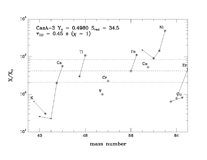
Figure 16: Production factors (final decayed mass fractions divided by their abundances in the Sun) representing the range of species produced in the $\alpha$-rich freeze-out from peak conditions for point CasA-3 in Table 5 assuming our ”recommended” reaction rates for ⁴⁰Ca($\alpha,\gamma$)⁴⁴Ti and ⁴⁴Ti($\alpha,p$)⁴⁷V. This is for the specific case of $Y_{e}=0.4980$ and $\chi=1$. This is a fairly typical nucleosynthesis pattern over the range of allowed $Y_{e}$ for the $\alpha$-rich freeze outs in the CasA and two-dimensional explosion models we consider.

⁴⁴Ti synthesis is also affected by the expansion timescale, $\tau_{\rm HD}=446\chi/\sqrt{\rho_{p}}$. Figure 16 shows the range of nuclei produced in an $\alpha$-rich freeze-out from peak conditions given for point CasA-3 in Table 5 with an initial composition of $Y_{e}=0.4980$ and our default scaling of $\chi=1$. The nucleosynthesis is presented in terms of ”traditional” production factors (so far our results have been expressed as ratios of production factors to that of ⁵⁶Fe). In the figure isotopes of a given element are connected by solid lines, those produced as radioactive progenitors are surrounded by a diamond, the most abundant isotope of a given element is denoted by a star. The dotted lines indicate a factor of 2 above and below the dashed line centered on ⁵⁶Fe (made as ⁵⁶Ni, ⁴⁴Ca is made as ⁴⁴Ti). The dominant species are in the iron group. This is a fairly typical result for any of the CasA or two-dimensional explosion model expansions within the allowed range of $Y_{e}$.

Figure 17 explores the effect of increasing the hydrodynamic time-scale by a factor of $\chi=5$. Shown is a straight forward ratio of ”traditional” production factors for the CasA-3 expansion assuming both the default ($\chi=1$) and extended ($\chi=5$) scaling on $\tau_{\rm HD}$. The species in the iron group are not much affected, ^56,58Ni are slightly higher than unity, all others show lower production factors. The reason is that for a longer expansion timescale, the material experiences higher temperatures for a longer duration. Those made dominantly in NSE (the iron group seen here) are slightly altered due to $\alpha$-particle reactions on them, which are ultimately provided by photo-disintegration and operation of the $3\alpha$-reaction. The effect is to reduce the overall fraction of $\alpha$-particles available at late times for the re-assembly of species lighter than the iron group.

Figure 18 shows for the specific CasA-3 example above the temperature evolution over the first 4 s assuming the two scalings. Over that time the temperature in the default ($\chi=1$, dotted line) scenario declined from $T_{9}=4.7$ - 0.25 while the longer expansion ($\chi=5$, dashed line) only declined to $T_{9}=2.6$. Also shown is the ratio of the $\alpha$-particle mass fraction (long/default). Recall that both ⁴⁰Ca and ⁴⁴Ti begin to re-assemble below $T_{9}=4$ (Figure 15). By the time the longer expansion scenario reaches $T_{9}=4$, it only has 65% of the $\alpha$-particle mass fraction that the default expansion had, by $T_{9}=3$ it is down to 52%. With only half the $\alpha$-particles to work with, the expansion with the higher scaling only reached $P_{44}=0.5\pm 0.1$, a factor of 2.6 less than the default expansion. Figure 19 shows the effect over all scenarios considered in the CasA model expansions. The average $P_{44}$ for points 4-6 (the two-dimensional explosion model) were 0.1, 0.05, and 0.08, respectively, over the allowed range of $Y_{e}$. For points 7 and 8 they are essentially zero.

5 Conclusions

We have considered the sensitivity to ⁴⁴Ti production in expansions that approximate freeze outs from NSE due to variations in the principle production and destruction reactions ⁴⁰Ca($\alpha,\gamma$)⁴⁴Ti and ⁴⁴Ti($\alpha,p$)⁴⁷V, and contrast them to experimental and theory reaction rate developments over the past 20 years. Experimentally we have also measured a thick-target yield for the ⁴⁰Ca($\alpha$,$\gamma$)⁴⁴Ti reaction. In-beam $\gamma$-ray spectroscopy was used to determine the yield of the 1083 keV prompt $\gamma$-ray from ⁴⁴Ti at $E_{\alpha}$ = 4.13, 4.54, and 5.36 MeV. In order to correct for those transitions which bypass the 1083 keV transition, the Monte Carlo code DICEBOX was used to estimate a correction of 20$\%$ to the in-beam thick target yield. An off-line activation measurement using the target from the $E_{\alpha}$ = 5.36 MeV irradiation showed good agreement with the in-beam measurement.

We then derived a thermonuclear reaction rate by normalizing the NON-SMOKER cross section (down by a factor of 1.71) to agree with our measured off-line thick target yield. We derived an error bar for our recommended rate whose magnitude ($\pm\times 2$) was dominated by the theoretical cross section error. We also carry out a similar re-evaluation of the ⁴⁴Ti($\alpha,p$)⁴⁷V reaction rate whose cross section was measured by Sonzogni et al. (2000). For both reactions, we conclude that the experimental data were far above the Gamow window, and suggest that further measurements be attempted.

We then carried out a sensitivity survey of ⁴⁴Ti nucleosynthesis in adiabatic expansions from eight peak temperature and density combinations drawn from conditions in three recent stellar explosion models (Magkotsios et al., 2008). For each expansion we survey a range of initial compositions ($0.505\geq Y_{e}\geq 0.485$). We also vary the principle production and destruction rates affecting ⁴⁴Ti in these expansions (eight choices of production rate, four for destruction). Our results show ⁴⁴Ti produced in proportion to solar iron for only one expansion drawn from a model for Cassiopia A, even though the final mass fractions for ⁴⁴Ti in most of the expansions are typically of order $10^{-4}$. With one exception, the other expansions are consistent with ⁴⁴Ti production seen in previous surveys of one-dimensional stellar evolution and with constraints imposed by solar abundances. Our results suggest that a strong $\alpha$-rich freeze out ($X(\alpha)_{f}\sim 0.2-0.3$) is highly conducive to ⁴⁴Ti synthesis.

With respect to reaction rate sensitivity, our experimental results suggest a recommended ⁴⁰Ca($\alpha,\gamma$)⁴⁴Ti reaction rate that is smaller than those predicted by the most recent experimental efforts (Vockenhuber et al., 2007; Nassar et al., 2006), but with a fairly large error bar ($\pm\times 2$) that would in fact encompass the former one. Nucleosynthesis models using our recommended rate would suggest less ⁴⁴Ti than these two recent experiments, although it would be higher than that suggested by an earlier measured rate (Cooperman et al., 1977) and the current theory rate (Rauscher & Thielemann, 2000). The total range of sensitivity is a factor of 1.5 (36%) when considering all of the production rates available. We also find that the uncertainties associated with the dominant destruction rate, ⁴⁴Ti($\alpha,p$)⁴⁷V, have roughly double the impact on ⁴⁴Ti synthesis ($\times 3.2$, or 70%) than that exhibited by the entire range of production rates. We suggest the use of our re-evaluation of the only available experimental reaction rate (Sonzogni et al., 2000) and strongly suggest consideration of its attendant larger uncertainty ($\pm\times 3$). This is a slightly larger spread in ⁴⁴Ti sensitivity than observed in two recent surveys of massive star nucleosynthesis (Rauscher et al., 2002; Limongi & Chieffi, 2006) that used essentially the same nuclear data, suggesting that current uncertainties in reaction rates could lead to as large an uncertainty in ⁴⁴Ti synthesis as that produced by different treatments of stellar physics.

Since the seminal work of Woosley et al. (1973), several new and novel theories of SN nucleosynthesis have featured regimes within the neutrino wind where the $\alpha-$rich freeze out plays an important role, including scenarios for the $r$-process (Woosley et al., 1994; Hoffman et al., 1997), and the $\nu p$-process (Fröhlich et. al., 2006; Pruet et. al., 2006). In each a combination of high entropy $(S_{\rm rad}\geq 50)$ and short expansion time-scale are required to produce the unique signatures of each process (the $r$-abundances, and light $p$-nuclei, respectively). However, as a consequence of extreme neutrino irradiation, the composition is forced away from neutron-proton equality and ultimately high entropy material enters regions above the iron group where local effects due to rapid changes in particle separation energies have a strong influence on the net nuclear flows. In these works no ⁴⁴Ti is reported.

Further out in the SN ejecta theory does not show ⁴⁴Ti enhancement due to the $\nu$-process in massive stars (Woosley et al., 1990; Woosley et al., 1995), nor in recent low-mass (electron capture) core-collapse scenarios (Hoffman et al., 2008; Wanajo et al., 2009). The later has been shown to effectively synthesize the long elusive $\alpha$-rich freeze-out candidate ⁶⁴Zn, but not ⁴⁴Ti. Our limited survey suggests that ⁴⁴Ti synthesis requires modest entropy $(S_{\rm rad}\sim 35$) and expansion timescales ($\sim\tau_{\rm HD}=0.45$ s) over a fairly narrow range of $Y_{e}$ ($0.5\geq Y_{e}\geq 0.4980$).

To date surveys of massive star evolution and nucleosynthesis have typically underproduced species whose production is attributed to the $\alpha$-rich freeze-out, in particular ⁴⁴Ca (made as ⁴⁴Ti) and ⁶⁴Zn (Woosley et al., 1995; Limongi & Chieffi, 2006). This has largely been ascribed to variations in treatments of stellar physics, most notably the parameterization of the explosion in one-dimensional models. Incorporating stellar yields from these surveys into models for galactic chemical evolution indicate the degree of underproduction, roughly a factor of a $2-3$ (Timmes, Woosley, & Weaver, 1995). Recent work has lead to models for the progenitor of Cassiopia A that suggest increased production, but the underlying physics is still quite uncertain and in need of improvement (Young et al., 2006). Future attention may focus on issues related to asymmetrical explosions where a noted increase in ⁴⁴Ti production compared to models with imposed spherical symmetry has been suggested for many years (Nagataki et al., 1997; Nagataki et al., 1998; Hwang & Laming, 2003; Young et al., 2006). The community is on the threshold of three-dimensional calculations that should provide valuable insight into the core-collapse mechanism, including physics such as rotation and magnetic fields which will likely enforce an asymmetrical result. Such results should help guide future parameterizations of the explosion in our one-dimensional models which will continue to carry the burden in future surveys of massive star evolution and nucleosynthesis. We believe we have addressed the uncertainty in two key nuclear reaction rates affecting ⁴⁴Ti synthesis, but ultimately, if Type II SNe are the dominant site of ⁴⁴Ti production, future models will have to include a larger fraction of their ejecta that experience an $\alpha$-rich freeze out than they have in the past. Another solution would be an additional source of ⁴⁴Ti, such as rare SNe of type Ia (Woosley et al., 1986; Woosley, 1997) or Ib (Perets et al., 2010).

Table 6. Nucleosynthesis Survey1
$Y_{e}$	0.5050	0.5000	0.4995	0.4990	0.4985	0.4980	0.4965	0.4950	0.4900	0.4850
$\eta$	-0.0100	0.0000	0.0010	0.0020	0.0030	0.0040	0.0070	0.0100	0.0200	0.0300
Point 1: Model for Cassiopia A, $T_{9p}=6.5,\rho_{p}=4.0\times 10^{6}$, S${}_{\rm rad}=22.8,\tau_{\rm HD}=0.22$ s
$X(\alpha$)	2.06(-1)	2.08(-1)	2.07(-1)	2.06(-1)	2.04(-1)	2.03(-1)	1.98(-1)	1.94(-1)	1.79(-1)	1.64(-1)
$X(^{40}$Ca)	1.66(-4)	8.27(-4)	7.87(-4)	7.46(-4)	7.15(-4)	6.89(-4)	6.26(-4)	5.72(-4)	4.25(-4)	1.00(-4)
$X(^{44}$Ti)	6.17(-5)	3.00(-4)	3.49(-4)	3.42(-4)	3.34(-4)	3.27(-4)	3.05(-4)	2.85(-4)	2.22(-4)	7.39(-5)
$X(^{56}$Ni)	7.51(-1)	7.35(-1)	7.17(-1)	6.92(-1)	6.66(-1)	6.39(-1)	5.58(-1)	4.77(-1)	2.11(-1)	4.58(-3)
$X(^{57}$Ni)	2.09(-3)	1.22(-2)	2.89(-2)	3.09(-2)	3.27(-2)	3.42(-2)	3.78(-2)	3.98(-2)	3.48(-2)	4.52(-3)
$X(^{58}$Ni)	2.25(-5)	1.57(-3)	9.70(-3)	3.50(-2)	6.04(-2)	8.59(-2)	1.63(-1)	2.41(-1)	5.08(-1)	6.97(-1)
$P_{44}$	0.062	0.305	0.364	0.369	0.374	0.382	0.409	0.446	0.786	12.027
$P_{57}$	0.131	0.707	1.717	1.891	2.079	2.283	2.889	3.536	7.024	42.192
$P_{58}$	0.004	0.221	0.309	1.153	2.060	3.071	6.659	11.504	54.762	3452.055
Point 2: Model for Cassiopia A, $T_{9p}=5.5,\rho_{p}=2.0\times 10^{6}$, S${}_{\rm rad}=27.7,\tau_{\rm HD}=0.32$ s
$X(\alpha$)	2.22(-1)	2.25(-1)	2.25(-1)	2.23(-1)	2.22(-1)	2.21(-1)	2.16(-1)	2.12(-1)	1.98(-1)	1.84(-1)
$X(^{40}$Ca)	2.47(-4)	9.50(-4)	9.06(-4)	8.61(-4)	8.27(-4)	7.99(-4)	7.30(-4)	6.73(-4)	5.15(-4)	1.04(-4)
$X(^{44}$Ti)	8.66(-5)	3.59(-4)	4.14(-4)	4.06(-4)	3.98(-4)	3.90(-4)	3.68(-4)	3.46(-4)	2.80(-4)	8.13(-5)
$X(^{56}$Ni)	7.35(-1)	7.17(-1)	6.99(-1)	6.75(-1)	6.48(-1)	6.22(-1)	5.40(-1)	4.59(-1)	1.92(-1)	3.06(-3)
$X(^{57}$Ni)	2.18(-3)	1.22(-2)	2.82(-2)	3.00(-2)	3.17(-2)	3.32(-2)	3.65(-2)	3.82(-2)	3.25(-2)	3.17(-3)
$X(^{58}$Ni)	2.53(-5)	2.03(-3)	1.00(-2)	3.54(-2)	6.09(-2)	8.64(-2)	1.64(-1)	2.42(-1)	5.09(-1)	6.57(-1)
$P_{44}$	0.088	0.374	0.441	0.450	0.458	0.468	0.508	0.562	1.085	19.836
$P_{57}$	0.132	0.721	1.715	1.884	2.078	2.267	2.867	3.534	7.190	44.672
$P_{58}$	0.004	0.216	0.328	1.198	2.136	3.178	6.900	12.000	60.261	4877.049
Point 3: Model for Cassiopia A, $T_{9p}=4.7,\rho_{p}=1.0\times 10^{6}$, S${}_{\rm rad}=34.5,\tau_{\rm HD}=0.45$ s
$X(\alpha$)	3.13(-1)	3.17(-1)	3.16(-1)	3.15(-1)	3.14(-1)	3.13(-1)	3.09(-1)	3.06(-1)	2.96(-1)	2.86(-1)
$X(^{40}$Ca)	7.70(-4)	2.10(-3)	2.04(-3)	1.94(-3)	1.87(-3)	1.82(-3)	1.69(-3)	1.59(-3)	1.31(-3)	1.85(-4)
$X(^{44}$Ti)	2.05(-4)	8.57(-4)	9.81(-4)	9.69(-4)	9.57(-4)	9.45(-4)	9.10(-4)	8.77(-4)	7.74(-4)	1.44(-4)
$X(^{56}$Ni)	6.40(-1)	6.17(-1)	5.99(-1)	5.75(-1)	5.49(-1)	5.22(-1)	4.41(-1)	3.60(-1)	9.43(-2)	2.56(-3)
$X(^{57}$Ni)	1.83(-3)	1.27(-2)	2.81(-2)	2.99(-2)	3.15(-2)	3.29(-2)	3.55(-2)	3.62(-2)	2.39(-2)	1.30(-3)
$X(^{58}$Ni)	2.21(-5)	2.56(-3)	8.26(-3)	3.29(-2)	5.77(-2)	8.26(-2)	1.58(-1)	2.34(-1)	4.94(-1)	4.31(-1)
$P_{44}$	0.238	1.037	1.223	1.258	1.300	1.349	1.543	1.818	6.120	41.053
$P_{57}$	0.123	0.878	1.994	2.210	2.454	2.675	3.429	4.266	10.787	22.010
$P_{58}$	0.003	0.243	0.315	1.304	2.408	3.614	8.171	14.825	119.333	3732.058
Point 4: Rotating Two-dimensional Explosion Model, $T_{9p}=6.5,\rho_{p}=1.0\times 10^{7}$, S${}_{\rm rad}=9.14,\tau_{\rm HD}=0.14$ s
$X(\alpha$)	1.03(-1)	1.06(-1)	1.05(-1)	1.04(-1)	1.03(-1)	1.02(-1)	9.77(-2)	9.39(-2)	8.14(-2)	6.95(-2)
$X(^{40}$Ca)	2.00(-5)	4.54(-4)	4.32(-4)	4.03(-4)	3.81(-4)	3.62(-4)	3.15(-4)	2.75(-4)	1.74(-4)	8.54(-5)
$X(^{44}$Ti)	3.11(-5)	1.34(-4)	1.90(-4)	1.83(-4)	1.77(-4)	1.70(-4)	1.51(-4)	1.34(-4)	8.76(-5)	4.87(-5)
$X(^{56}$Ni)	8.50(-1)	8.40(-1)	8.21(-1)	7.94(-1)	7.67(-1)	7.39(-1)	6.56(-1)	5.74(-1)	3.04(-1)	4.68(-2)
$X(^{57}$Ni)	4.15(-3)	1.13(-2)	2.79(-2)	3.07(-2)	3.32(-2)	3.55(-2)	4.07(-2)	4.40(-2)	4.30(-2)	1.98(-2)
$X(^{58}$Ni)	7.02(-5)	9.96(-4)	1.14(-2)	3.58(-2)	6.04(-2)	8.51(-2)	1.60(-1)	2.37(-1)	5.03(-1)	7.79(-1)
$P_{44}$	0.029	0.119	0.173	0.173	0.172	0.172	0.172	0.175	0.216	0.777
$P_{57}$	0.267	0.571	1.445	1.648	1.839	2.044	2.649	3.268	6.017	18.011
$P_{58}$	0.021	0.183	0.317	1.029	1.790	2.624	5.566	9.408	37.801	379.032
1 All results assume our ”recommended” rates for 40Ca($\alpha,\gamma$)44Ti and 44Ti($\alpha,p$)47V.

Table 6. Nucleosynthesis Survey1 (continued)
$Y_{e}$	0.5050	0.5000	0.4995	0.4990	0.4985	0.4980	0.4965	0.4950	0.4900	0.4850
$\eta$	-0.0100	0.0000	0.0010	0.0020	0.0030	0.0040	0.0070	0.0100	0.0200	0.0300
Point 5: Rotating Two-dimensional Explosion Model, $T_{9p}=5.5,\rho_{p}=1.0\times 10^{7}$, S${}_{\rm rad}=5.54,\tau_{\rm HD}=0.14$ s
$X(\alpha$)	6.85(-2)	7.23(-2)	7.17(-2)	7.07(-2)	6.96(-2)	6.85(-2)	6.53(-2)	6.21(-2)	5.23(-2)	4.36(-2)
$X(^{40}$Ca)	1.13(-5)	3.68(-4)	3.56(-4)	3.29(-4)	3.08(-4)	2.90(-4)	2.46(-4)	2.10(-4)	1.23(-4)	6.11(-5)
$X(^{44}$Ti)	1.61(-5)	8.16(-5)	1.62(-4)	1.54(-4)	1.47(-4)	1.41(-4)	1.22(-4)	1.05(-4)	6.34(-5)	3.43(-5)
$X(^{56}$Ni)	8.77(-1)	8.74(-1)	8.54(-1)	8.27(-1)	7.99(-1)	7.71(-1)	6.87(-1)	6.04(-1)	3.31(-1)	6.85(-2)
$X(^{57}$Ni)	7.18(-3)	9.75(-3)	2.59(-2)	2.92(-2)	3.22(-2)	3.48(-2)	4.08(-2)	4.45(-2)	4.47(-2)	2.40(-2)
$X(^{58}$Ni)	1.86(-4)	8.99(-4)	1.18(-2)	3.54(-2)	5.92(-2)	8.33(-2)	1.57(-1)	2.32(-1)	4.95(-1)	7.73(-1)
$P_{44}$	0.015	0.070	0.142	0.139	0.137	0.136	0.132	0.130	0.143	0.373
$P_{57}$	0.451	0.474	1.291	1.502	1.717	1.928	2.527	3.125	5.741	14.926
$P_{58}$	0.056	0.157	0.316	0.977	1.685	2.467	5.201	8.771	34.144	257.353
Point 6: Rotating Two-dimensional Explosion Model, $T_{9p}=4.7,\rho_{p}=1.0\times 10^{7}$, S${}_{\rm rad}=3.45,\tau_{\rm HD}=0.14$ s
$X(\alpha$)	5.67(-2)	6.07(-2)	6.04(-2)	5.97(-2)	5.90(-2)	5.84(-2)	5.65(-2)	5.48(-2)	4.99(-2)	4.58(-2)
$X(^{40}$Ca)	1.36(-5)	4.91(-4)	5.04(-4)	4.67(-4)	4.42(-4)	4.20(-4)	3.71(-4)	3.32(-4)	2.36(-4)	1.46(-4)
$X(^{44}$Ti)	1.19(-5)	6.90(-5)	2.42(-4)	2.33(-4)	2.24(-4)	2.17(-4)	1.96(-4)	1.79(-4)	1.34(-4)	9.15(-5)
$X(^{56}$Ni)	8.68(-1)	8.76(-1)	8.56(-1)	8.28(-1)	7.99(-1)	7.71(-1)	6.86(-1)	6.02(-1)	3.26(-1)	6.19(-2)
$X(^{57}$Ni)	1.14(-2)	8.83(-3)	2.47(-2)	2.85(-2)	3.18(-2)	3.46(-2)	4.09(-2)	4.46(-2)	4.42(-2)	2.28(-2)
$X(^{58}$Ni)	4.46(-4)	8.06(-4)	1.05(-2)	3.22(-2)	5.43(-2)	7.66(-2)	1.45(-1)	2.15(-1)	4.59(-1)	7.14(-1)
$P_{44}$	0.011	0.059	0.210	0.210	0.209	0.209	0.213	0.222	0.306	1.102
$P_{57}$	0.720	0.428	1.229	1.464	1.685	1.912	2.532	3.159	5.753	15.650
$P_{58}$	0.139	0.143	0.281	0.888	1.550	2.271	4.826	8.159	32.124	262.195
Point 7: Rotating Two-dimensional MHD Model (CHASM region), $T_{9p}=6.5,\rho_{p}=1.0\times 10^{8}$, S${}_{\rm rad}=0.91,\tau_{\rm HD}=0.04$ s
$X(\alpha$)	1.01(-2)	1.31(-2)	1.20(-2)	1.08(-2)	9.65(-3)	8.51(-3)	5.25(-3)	2.26(-3)	1.81(-6)	8.95(-7)
$X(^{40}$Ca)	7.43(-8)	3.61(-5)	2.64(-5)	1.94(-5)	1.41(-5)	9.95(-6)	2.68(-6)	2.88(-7)	4.06(-8)	2.35(-7)
$X(^{44}$Ti)	1.22(-7)	1.15(-5)	1.11(-5)	8.25(-6)	5.97(-6)	4.19(-6)	1.08(-6)	1.06(-7)	1.98(-9)	6.31(-9)
$X(^{56}$Ni)	8.67(-1)	9.40(-1)	9.14(-1)	8.87(-1)	8.59(-1)	8.32(-1)	7.52(-1)	6.71(-1)	3.93(-1)	1.28(-1)
$X(^{57}$Ni)	1.06(-2)	1.34(-2)	2.30(-2)	2.84(-2)	3.30(-2)	3.69(-2)	4.57(-2)	5.15(-2)	4.88(-2)	3.07(-2)
$X(^{58}$Ni)	7.53(-4)	1.50(-4)	1.92(-2)	4.21(-2)	6.61(-2)	9.11(-2)	1.72(-1)	2.60(-1)	4.30(-1)	5.61(-1)
$P_{44}$	0.000	0.009	0.009	0.007	0.005	0.004	0.001	0.000	0.000	0.000
$P_{57}$	1.327	0.607	1.069	1.365	1.642	1.891	2.596	3.265	5.272	10.388
$P_{58}$	1.244	0.064	0.478	1.082	1.760	2.496	5.209	8.837	24.888	99.029
Point 8: Rotating Two-dimensional MHD Model, $T_{9p}=5.5,\rho_{p}=1.0\times 10^{8}$, S${}_{\rm rad}=0.55,\tau_{\rm HD}=0.04$ s
$X(\alpha$)	9.27(-3)	1.13(-2)	1.07(-2)	9.89(-3)	9.16(-3)	8.47(-3)	6.57(-3)	4.86(-3)	4.69(-4)	2.45(-6)
$X(^{40}$Ca)	1.39(-7)	5.28(-5)	4.50(-5)	3.56(-5)	2.84(-5)	2.27(-5)	1.12(-5)	4.92(-6)	1.59(-8)	4.70(-10)
$X(^{44}$Ti)	2.14(-7)	6.95(-6)	2.06(-5)	1.65(-5)	1.33(-5)	1.07(-5)	5.20(-6)	2.24(-6)	5.93(-9)	4.65(-11)
$X(^{56}$Ni)	7.86(-1)	9.25(-1)	9.01(-1)	8.74(-1)	8.47(-1)	8.20(-1)	7.39(-1)	6.59(-1)	3.89(-1)	1.18(-1)
$X(^{57}$Ni)	1.07(-2)	8.79(-3)	2.10(-2)	2.67(-2)	3.14(-2)	3.52(-2)	4.39(-2)	4.95(-2)	5.37(-2)	3.37(-2)
$X(^{58}$Ni)	1.40(-3)	2.13(-4)	1.47(-2)	3.50(-2)	5.64(-2)	7.89(-2)	1.52(-1)	2.32(-1)	5.45(-1)	7.60(-1)
$P_{44}$	0.000	0.006	0.017	0.014	0.012	0.010	0.005	0.003	0.000	0.000
$P_{57}$	1.505	0.404	0.992	1.298	1.575	1.828	2.521	3.193	5.890	12.301
$P_{58}$	2.660	0.086	0.373	0.914	1.516	2.197	4.685	8.031	31.974	146.341
1 All results assume our ”recommended” rates for 40Ca($\alpha,\gamma$)44Ti and 44Ti($\alpha,p$)47V.

Figure 2: A Schematic of the target chamber used in the experiment.

Figure 3: Partial HPGe $\gamma$-ray spectra at $E_{\alpha}$ = 5.36 for the detector at 99^∘ with a simultaneous fit to the 1039 keV ⁷⁰Ge and 1083 keV ⁴⁴Ti $\gamma$-rays.

Figure 5: $\gamma$-ray spectra observed in a two week low background count of the activated target bombarded at $E_{\alpha}$ = 5.36 MeV.

Figure 6: The Effective Gamow windows for ⁴⁰Ca($\alpha$,$\gamma$)⁴⁴Ti and ⁴⁴Ti($\alpha,p$)⁴⁷V at $T_{9}=2$ and $T_{9}=5$. Shown are the true Gamow window as given by the real integrand of the reaction rate formula (solid line type, see Eq. 4), the product of the high-energy tail of the Maxwell-Boltzmann distribution with the simple Coulomb barrier penetration factor (denoted as “exp(-E/kT-b/sqrt(E)), dot-dash line type)” and the usual Gaussian approximation to the latter (“Gauss approx”, dotted line type). Stars denote the energy values at which experimental data were measured in our effort and from Sonzogni et al. (2000). The Gaussian approximation is widely used to estimate the Gamow window but predicts it at too high an energy, especially for the capture reaction. For purposes of illustration, all curves were renormalized to the arbitrary unit scale shown, for $T_{9}=5$ all three quantities peak at 10, for $T_{9}=2$ they peak at 6.

Figure 7: Comparison of the experimental energy range for ⁴⁰Ca($\alpha$,$\gamma$)⁴⁴Ti with the true Gamow window given by the actual maximal contributions to the reaction rate integral. The experimental data do not contribute significantly to the rate in the temperature range relevant to ⁴⁴Ti synthesis ($2.0\leq{\rm T}_{9}\leq 4.0$).

Figure 9: Fits to reaction rates for ⁴⁰Ca($\alpha$,$\gamma$)⁴⁴Ti considered in this study. Solid and dashed line types denote experimental rates from various authors, dotted and dot-dash line types are from various theory efforts. The tabulated NON-SMOKER theory rate (Rauscher & Thielemann, 2001) is denoted by crosses. Our recommended rate (and its error, $\pm\times 2$) are indicated as solid (lighter) lines. The inset illustrates the ratio of each reaction rate to the NON-SMOKER rate, including the (dot-short-dash) original fit (Rauscher & Thielemann, 2000), our attempt (dotted) to refit the tabulated NON-SMOKER rate, and the theory rate (dot-long-dash) of Woosley et al. (1978).

Figure 11: Re-evaluated ⁴⁴Ti($\alpha$,$p$)⁴⁷V rate, based on data by Sonzogni et al. (2000): Ratio of the new rate to the NON-SMOKER rate (Rauscher & Thielemann, 2001). The estimated range of the rate is derived from the theoretical and experimental errors (see the text for details). The geometric mean of the upper and lower limit is used as a recommended rate in this work. The impact of the Sonzogni et al. (2000) data manifests itself in the deviation of the geometric mean from unity. Within errors, the new rate is compatible with the NON-SMOKER rate.

Figure 12: Normalized production factors for ⁴⁴Ti, ⁵⁷Ni and ⁵⁸Ni versus initial stellar mass derived from nucleosynthetic yields of SN models (Woosley et al., 1995; Rauscher et al., 2002; Limongi & Chieffi, 2006; Young et al., 2006).

Figure 13: Normalized production factors for ⁴⁴Ti, ⁵⁷Ni, and ⁵⁸Ni versus $Y_{e}$ for adiabatic freeze outs from peak conditions CasA $1-3$ in Table 5. All points were drawn from a model for Cassiopia A (Magkotsios et al., 2008). Each central point represents a calculation that utilizes our recommended ”semi-experimental” reaction rate for ⁴⁰Ca($\alpha,\gamma$)⁴⁴Ti and three choices of ⁴⁴Ti($\alpha,p$)⁴⁷V reaction rate from our re-evaluation of the experimental effort of Sonzogni et al. (2000): our ”recommended” ⁴⁴Ti($\alpha,p$)⁴⁷V rate (solid line, filled squares), and its upper and lower bound (denoted by filled triangles with dotted and dashed line styles, respectively). Error bars on each point reflect the minimum and maximum deviations of $P_{44}$ due to variations of the six other ⁴⁰Ca($\alpha,\gamma$)⁴⁴Ti reaction rates we considered. The dot-short-dash line shows ⁴⁴Ti synthesis using the original fits of Rauscher & Thielemann (2000) for both ⁴⁰Ca($\alpha,\gamma$)⁴⁴Ti and ⁴⁴Ti($\alpha,p$)⁴⁷V. For the two NPF’s $P_{57}$ and $P_{58}$ (shown as open and filled circles, respectively) an upper bound of 3 limits the allowed range of $Y_{e}$.

Figure 14: Same as Figure 13 but for peak conditions $4-6$ in Table 5 drawn from a rotating two-dimensional explosion model (Magkotsios et al., 2008). The production of ^57,58Ni with respect to solar iron is nearly the same as in the model for CasA, but the production of ⁴⁴Ti is substantially lower in every case due to the lower entropy experienced in these expansions.

Figure 15: Evolution of select mass fractions versus temperature during freeze outs with identical peak temperatures ($T_{9p}=5.5$) and electron fractions ($Y_{e}=0.4980$), but different intial peak densities, for three points in our survey. The higher entropy expansions produce less ⁵⁶Ni and have a higher $\alpha$-particle mass fraction at late times that facilitates the re-assembly of species below the iron group, including ⁴⁰Ca and ⁴⁴Ti.

Figure 17: Similar to Figure 16, this is the ratio of the production factors for two scalings on the hydrodynamic time-scale, default ($\chi=1$) and extended ($\chi=5$). The species created in NSE are much less affected than the lighter isotopes which are reassembled for $2\leq T_{9}\leq 4$.

Figure 18: Temperature evolution in the CasA-3 expansion assuming two scalings on the hydrodynamic time-scale, default ($\chi=1$) and extended ($\chi=5$). Also shown is the ratio of the $\alpha$-particle mass fraction.

Figure 19: Normalized production factors for ⁴⁴Ti, ⁵⁷Ni, and ⁵⁸Ni versus $Y_{e}$ for adiabatic freeze outs from peak conditions CasA $1-3$ in Table 5 but with an assumed $\chi=5$ scaling of the hydrodynamic timescale. Results for the Ni isotopes are very similar to the default ($\chi=1$) scaling case (Figure 13), but due to the longer time spent at high temperature, the $\alpha$-particle abundance at the onset of ⁴⁰Ca assembly was much lower ($\sim 40$%) than in the default scaling case, which facilitated a much lower final value for $P_{44}$ in all cases studied.

References

- Ahmad et al. (2006) Ahmad, I. et al. 2006, Phys. Rev., C74, 065802
- Becvar (1998) Becvar, F. 1998, Nucl. Instrum. Methods Phys. Res. A, 471, 434 (DICEBOX)
- Caughlan & Fowler (1998) Caughlan, G. R., & Fowler, W. A. 1988, At. Data Nucl. Data Tables, 40, 283
- Clayton (1984) Clayton, D. D. 1984, Principles of Stellar Evolution and Nucleosynthesis (Univ. Chicago Press) Chicago, London
- Cooperman et al. (1977) Cooperman, E. et al. 1977, Nucl. Phys., A284, 284
- Czosnyka et al. (1983) Czosnyka, T. et al. 1983, Am. Phys. Soc., 28, 745
- Diehl et al. (2006) Diehl, R. et al. 2006, Nucl. Phys., A777, 70
- Dyer et al. (1981) Dyer, P. et al. 1981, Phys. Rev., C23, 1865
- Fisker et al. (2001) Fisker, J. L. et. al. 2001, At. Data Nucl. Data Tables, 79, 241
- Fowler, Caughlan & Zimmerman (1967) Fowler, W. A., Caughlan, G. R., & Zimmerman, B. A. 1967, ARA&A, 5, 525
- Fröhlich et. al. (2006) Fröhlich, C., Martínez-Pinedo, G., Liebendörfer, M., Thielemann, F.-K., Bravo, E., Hix, W. R., Langanke, K.-H., & Zinner, N. T. 2006, Phys. Rev. Lett. 96, 142502
- Gete et al. (1997) Gete, E. et al. 1997, Nucl. Instrum. Methods Phys. Res. A, 388, 212
- Hartmann, Woosley, & El Eid (1985) Hartmann, D., Woosley, S. E., & El Eid, M. F. 1985, ApJ, 297, 837
- Hoffman et al. (1997) Hoffman, R. D., Woosley, S. E., & Qian, Y.-Z. 1997, ApJ, 482, 951
- Hoffman et al. (2002) Hoffman, R. D. et al. 2002, RateTable v. 8.2, http://adg.llnl.gov/Research/RRSN/
- Hoffman et al. (2008) Hoffman, R. D., Muller, B, & Janka, H. T. 2008, ApJ, L676, 127
- Holmes et al. (1976) Holmes, J. A. et al. 1976, At. Data Nucl. Data Tables, 18, 306
- Hsu (1982) Hsu, H. H. 1982, Nucl. Instrum. Methods, 193, 383
- Hwang & Laming (2003) Hwang, U., & Laming, J. M. 2003, ApJ, 597, 362
- Iliadis (2007) Iliadis, C. 2007, Nuclear Physics of Stars (Wiley-VCH), Berlin
- Iyudin et al. (1994) Iyudin, A. F. et al. 1994, A&A, 284, L1
- Iyudin et al. (1998) —. 1998, Nature, 396, 142
- Kiss et. al. (2008) Kiss, G. G., Rauscher, T., Gyürky, Gy., Simon, A., Fülöp, Zs., & Somorjai, E. 2008, Phys. Rev. Lett. 101, 191101
- Limongi & Chieffi (2006) Limongi, M. & Chieffi, A. 2006, ApJ, 647, 483
- Lodders (2003) Lodders, K. 2003, ApJ, 591, 1220
- Magkotsios et al. (2008) Magkotsios, G. L. et al. 2008, in Proc. 10th Symp. Nuclei in the Cosmos (NIC X), 112
- Nagataki et al. (1997) Nagataki, S., Hashimoto, M.-A., Sato, K., & Yamada, S. 1997, ApJ, 486, 1026
- Nagataki et al. (1998) Nagataki, S., Hashimoto, M.-A., Sato, K., Yamada, S., & Mochizuki, Y. S. 1998, ApJ, 492, L45
- Nassar et al. (2006) Nassar, H. et al. 2006, Phys. Rev. Lett., 96, 041102
- Perets et al. (2010) Perets, H. B. et. al. 2010, Nature, in press, http://adsabs.harvard.edu/abs/2009arXiv0906.2003P
- Pruet et. al. (2006) Pruet, J., Hoffman, R. D., Woosley, S. E., Janka, H.-T., & Buras, R., 2006, ApJ, 644, 1028
- Rauscher (2010) Rauscher, T. 2010, Phys. Rev. C, 81, 4, http://link.aps.org/doi/10.1103/PhysRevC.81.045807
- Rauscher (2003-2009) Rauscher, T. 2003-2009, Code EXP2RATE, http://download.nucastro.org/codes/exp2rate.f
- Rauscher & Thielemann (2000) Rauscher, T. & Thielemann, F. 2001, At. Data Nucl. Data Tables, 75, 1
- Rauscher & Thielemann (2001) —. 2001, At. Data Nucl. Data Tables, 79, 47
- Rauscher et al. (2000) Rauscher, T. et al. 2000, Nucl. Phys., A675, 695
- Rauscher et al. (2002) Rauscher, T. et al. 2002, ApJ, 576, 323
- Rauscher et al. (2009) Rauscher, T. et al. 2009, Phys. Rev., C80, 035801
- Renaud et al. (2006) Renaud, M. et al. 2006, ApJ, 647, L41
- Roughton et al. (1976) Roughton, N. A., Fritts, M. J., Peterson, R. J., Zaidins, C. S., and Hansen, C. J. 1976, ApJ, 205, 302
- Seitenzahl et al. (2008) Seitenzahl, I. R., Timmes, F. X., Marin-Lafleche, A., Brown, E., Magkotsios, G., and Truran, J. 2008, ApJ, 685L, 129S
- Simpson et al. (1971) Simpson, J. et al. 1971, Phys. Rev., C4, 443
- Sonzogni et al. (2000) Sonzogni, A. A. et al. 2000, Phys. Rev. Lett., 84, 1651
- The et al. (1998) The, L. S. et al. 1998, ApJ, 504, 500
- The et al. (2006) The, L.-S. et al. 2006, A&A, 450, 1037
- Thielemann, Arnould, & Truran (1987) Thielemann, F.-K., Arnould, M., & Truran, J. 1987, in Advances in Nuclear Astrophysics, ed. E. Vangioni-Flam (Gif-sur-Yvette: Editions Frontiere), 525
- Thielemann, Nomoto, & Hashimoto (1996) Thielemann, F.-K., Nomoto, K., & Hashimoto, M. 1996, ApJ, 460, 408
- Timmes, Woosley, & Weaver (1995) Timmes, F. X., Woosley, S. E., and Weaver, T. A. 1995, ApJS, 98, 617
- Timmes et al. (1996) Timmes, F. et al. 1996, ApJ, 464, 332
- Timmes (2010) Timmes, F., private communication, see also http://cococubed.asu.edu/code_pages/net_torch.shtml
- Vink et al. (2001) Vink, J. et al. 2001, ApJ, 560, L79
- Vockenhuber et al. (2007) Vockenhuber, C. et al. 2007, Phys. Rev., C76, 035801
- Wanajo et al. (2009) Wanajo, S. et al. (2009), ApJ, 695, 208
- Woosley (1997) Woosley, S. E. 1997, ApJ, 476, 801
- Woosley et al. (1986) Woosley, S. E., Taam, R. E., & Weaver, T. A. 1986, ApJ, 301, 601
- Woosley et al. (1973) Woosley, S. E., Arnett, D., & Clayton, D.D. 1973, ApJS, 26, 231
- Woosley et al. (1978) Woosley, S. E., Fowler, W. A., Holmes, J. A., & Zimmerman, B. A. 1978, Atomic Data & Nuclear Data Tables, 22, 371 - (see also ”Tables of Thermonuclear Reaction Rate Data for Intermediate Mass Nuclei”, OAP-422, (Caltech preprint, August 1975)
- Woosley et al. (1990) Woosley, S. E., Hartmann, D. H., Hoffman, R. D., & Haxton, W. C. 1990, ApJ, 365, 272
- Woosley et al. (1991) Woosley, S. E. & Hoffman, R. D. 1991, ApJ, 368, L31
- Woosley et al. (1994) Woosley, S. E., Wilson, J. R., Mathews G. J., Hoffman, R. D., & Meyer, B. S. 1994, ApJ, 433, 209
- Woosley et al. (1995) Woosley, S. E., & Weaver, T. 1995, ApJS, 101, 181
- Young et al. (2006) Young, P. A. et al. 2006, ApJ, 640, 891
- J.F. Ziegler (2004) Ziegler, J. F. 2004, Nucl. Instrum. Methods B, 219, 1027