Multiuser MIMO Downlink Beamforming Design Based on Group Maximum SINR Filtering

Abstract

In this paper we aim to solve the multiuser multi-input multi-output (MIMO) downlink beamforming problem where one multi-antenna base station broadcasts data to many users. Each user is assigned multiple data streams and has multiple antennas at its receiver. Efficient solutions to the joint transmit-receive beamforming and power allocation problem based on iterative methods are proposed. We adopt the group maximum signal-to-interference-plus-noise-ratio (SINR) filter bank (GSINR-FB) as our beamformer which exploits receiver diversity through cooperation between the data streams of a user. The data streams for each user are subject to an average SINR constraint, which has many important applications in wireless communication systems and serves as a good metric to measure the quality of service (QoS). The GSINR-FB also optimizes the average SINR of its output. Based on the GSINR-FB beamformer, we find an SINR balancing structure for optimal power allocation which simplifies the complicated power allocation problem to a linear one. Simulation results verify the superiority of the proposed algorithms over previous works with approximately the same complexity.

EDICS     MSP-MULT

I Introduction

In this paper, the joint beamforming and power allocation optimization problem for the multiuser multi-input multi-output (MIMO) downlink channel is considered. In this system, transmit and receive beamformings are used to suppress the multiuser interference and exploit the multi-antenna diversity. Power allocation at the transmitter is performed to efficiently utilize the available transmission power. Such a joint beamforming and power allocation problem has been studied by many researchers [1, 2, 3, 4, 5]. In [2][3], block diagonalization (BD) was proposed to block-diagonalize the overall channel so that the multiuser interference at each receiver is thoroughly eliminated. Such a zero-forcing approach suffers from the noise enhancement problem, because it removes the multiuser interference by ignoring the noise. Hence the performance can be improved if the balance between multiuser interference suppression and noise enhancement can be found [4][5].

Under individual signal-to-interference-plus-noise-ratio (SINR) constraints for users, Schubert and Boche studied the situation where each user has only one data stream and single receive antenna [4]. It was shown that the optimal solution can be efficiently found by iterative algorithms. Khachan et al. [5] generalized the scheme in [4] to allow several transmission beams to be grouped to serve a user, and each user has multiple receiver antennas [5]. However, each data stream is processed separately. Thus, in addition to the multiuser interference from the other users, there is intra-group interference between the data streams of a user. This drawback motivates our work to use a more sophisticated receiver processing to tackle the intra-group interference.

In this work, we adopt the group maximum SINR filter bank (GSINR-FB) proposed by [6] as the beamformer, which collects the desired signal energy in the streams of each user and maximize the total SINR at its output. That is, the GSINR-FB lets these streams cooperate while the filters in [5] let them compete. Based on the GSINR-FB beamformer, we consider a system which uses the average SINR over data streams for a user as a metric to measure the quality-of-service (QoS). This criterion is very useful in many communication scenarios [7, 8, 6] including the celebrated space-time block coded systems. It will be shown that the GSINR-FB based beamformer does improve the performance over the scheme in [5]. Moreover, we find that the SINR balancing structure exists for this beamforming method, that is, the optimal power allocation results in the same SINR to target ratio for all users with the GSINR-FB based beamforming. As will be shown later, this property makes solving the complicated power allocation problem much easier. Our work can be seen as a non-trivial generalization of [4] to the multi-antenna setting which also subsumes [5] as a special case (with independent processing of data streams). For simplicity, we will first consider group power allocation which restricts equal power on the data streams of each user to benefits from the low-complexity power allocation schemes similar to those in [4][5]. This restriction is later relaxed by allowing the power of individual data streams to be adjustable. Besides the GSINR-FB based beamforming, this per stream power allocation scheme is new compared with [4][5] and has better performance than the group power allocation. These two techniques are the key ingredients to make our performance better than that in [5]. With approximately the same complexity as [5], our approach exhibits a better performance compared to the existing methods in [5] and the BD based methods.

We will investigate two optimization problems. One is minimizing the total transmitted power while satisfying a set of average SINR targets. The other is maximizing the achieved average SINR to target ratio under a total power constraint. Based on the uplink-downlink duality [9], our methods iteratively calculate the GSINR-FB based beamforming and power allocation matrices. The rest of the paper is organized as follows. The system model and problem formulation are introduced in Section II. We also briefly discuss the basic design concept of our iterative algorithms in this section. Backgrounds such as the GSINR-FB based beamformers and the applications of the average SINR criterion are provided in Section III. Section IV presents our power allocation results. The numerical results are given in Section V, and the computational complexity issues are discussed in Section VI. Finally, we give the conclusion in VII.

II Problem Formulation and Efficient Iterative Solutions

II-A Notations

In this paper, vectors and matrices are denoted in bold-face lower and upper cases, respectively. For vector ${\mathbf{g}}$, ${\mathbf{g}}\geq_{e}0$ means that every element of ${\mathbf{g}}$ is nonnegative. For matrix $\mathbf{G}$, $\mathrm{trace}(\mathbf{G)}$ denotes the trace; $\mathbf{G}^{\mathrm{T}}$ and $\mathbf{G}^{H}$ denote the transpose and Hermitian operations, respectively. $\left\|\cdot\right\|_{F}$ denotes the Frobenius norm, which is defined as $\left\|{\bf{G}}\right\|_{F}=\sqrt{{\rm{trace}}\left({{\bf{GG}}^{H}}\right)}$. $\mathbf{G}_{s}^{-1}$ and $|\mathbf{G}_{s}|$ are, respectively, the inverse and determinant of a square matrix $\mathbf{G}_{s}.$ And $\mathbf{I}_{n}$ denotes the identity matrix of dimension $n$. A diagonal matrix is denoted $diag\{\ldots\}$ whose $k$th parameter is the $k$th diagonal term in the matrix. $E[\cdot]$ denotes the expectation operator.

II-B System Model

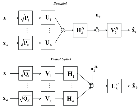
Figure 1: MIMO downlink system model for user $k$ and its virtual uplink.

Consider the downlink scenario with $K$ users, where a base station is equipped with $M$ antennas. The upper part of Fig. 1 shows the overall system block diagram for user $k$, who has $N_{k}$ receive antennas and receives $L_{k}$ data streams, where $L_{k}$ satisfies the constraint $L_{k}\leq\min\left\{M,N_{k}\right\}$ to make sure effective recovery of the data streams at the receiver. Thus the $K$ users have a total of $N=\sum\nolimits_{k=1}^{K}{N_{k}}$ receive antennas receiving a total of $L=\sum\nolimits_{k=1}^{K}{L_{k}}$ grouped data streams. For a given symbol time, the data streams intended for user $k$ are denoted by a vector of symbols $\mathbf{x}_{k}=[x_{k1},x_{k2},...,x_{kL_{k}}]^{T}$. The $L$ data streams are concatenated in a vector $\mathbf{x}=[\mathbf{x}^{T}_{1},...,\mathbf{x}^{T}_{K}]^{T}$. Without loss of generality, we assume that ${\mathbf{x}}$ is zero mean with covariance matrix ${\mathbf{I}}_{L}$. The precoder $\mathbf{U}_{k}\in\mathcal{C}^{M\times L_{k}}$ processes user $k$’s data streams before they are transmitted over the $M$ antennas. These individual precoders together form the $M\times L$ global transmitter beamforming matrix $\mathbf{U}=[\mathbf{U}_{1},\mathbf{U}_{2},...,\mathbf{U}_{K}]$. The power allocation matrix for user $k$ is a diagonal matrix

$$\mathbf{P}_{k}=diag\{p_{k1},p_{k2},...,p_{kL_{k}}\},$$ (1)

where $p_{kj}$ is the power allocated to the $j$th data stream of user $k$, and the global power allocation matrix

$$\mathbf{P}=diag\{\mathbf{P}_{1},\mathbf{P}_{2},...,\mathbf{P}_{K}\}$$ (2)

is a block diagonal matrix of dimension $L\times L$. The transmitter broadcasts signals $\mathbf{U\sqrt{P}x}$ to all of the $K$ users.

User $k$ receives a length $N_{k}$ vector ${\bf{y}}_{k}=\mathbf{H}^{H}_{k}\mathbf{U\sqrt{P}x}$, which can be expanded as

$${\bf{y}}_{k}={\bf{H}}_{k}^{H}{\bf{U}}_{k}\sqrt{{\bf{P}}_{k}}{\bf{x}}_{k}+{\bf{H}}_{k}^{H}\left({\sum\limits_{j\neq k,j=1}^{K}{{\bf{U}}_{j}\sqrt{{\bf{P}}_{j}}{\bf{x}}_{j}}}\right)+{\bf{n}}_{k},$$ (3)

where the channel between the transmitter and user $k$ is represented by the $N_{k}\times M$ matrix $\mathbf{H}_{k}^{H}$, the Hermitian of $\mathbf{H}_{k}$; $\mathbf{n}_{k}$ represents the zero-mean additive white Gaussian noise (AWGN) at user $k$’s receive antennas with variance $\sigma^{2}$ per antenna and the covariance matrix $E[\mathbf{n}_{k}\mathbf{n}_{k}^{H}]=\sigma^{2}\mathbf{I}_{N_{k}}$. The resulting $N\times M$ global channel matrix is $\mathbf{H}^{H}$, with $\mathbf{H}=[\mathbf{H}_{1},\mathbf{H}_{2},...,\mathbf{H}_{K}]$. We assume that the transmitter has perfect knowledge of the channel matrix $\mathbf{H}$, and receiver $k$ knows its $\mathbf{H}_{k}$ perfectly. The second term on the right-hand-side of (3) is the inter-group multiple user interference for user $k$. To estimate its $L_{k}$ symbols $\mathbf{x}_{k}$, user $k$ processes $\mathbf{y}_{k}$ with its $L_{k}\times N_{k}$ receive beamforming matrix $\mathbf{V}_{k}^{H}$. The resulting estimated signal vector is

$${\mathbf{\hat{x}}}_{k} ={\mathbf{V}}_{k}^{H}{\mathbf{H}}_{k}^{H}{\mathbf{U\sqrt{P}x}}+{\mathbf{V}}_{k}^{H}{\mathbf{n}}_{k}$$

$$=\mathbf{V}_{k}^{H}{\bf{H}}_{k}^{H}{\bf{U}}_{k}\sqrt{{\bf{P}}_{k}}{\bf{x}}_{k}+\mathbf{V}_{k}^{H}{\bf{H}}_{k}^{H}\left({\sum\limits_{j\neq k,j=1}^{K}{{\bf{U}}_{j}\sqrt{{\bf{P}}_{j}}{\bf{x}}_{j}}}\right)+\mathbf{V}_{k}^{H}{\bf{n}}_{k}.$$ (4)

Without loss of generality, as [6], we assume that the interference-plus-noise components of the filter bank output in (4) are uncorrelated. For any filter bank that produces correlated components, one can easily find another filter bank which makes these component uncorrelated but with the same performance. The details can be found in [6].

Finally, owing to the non-cooperative nature between users in broadcast channels, the global receiver beamforming filter $\mathbf{V}^{H}$, formed by collecting the individual receiver filters, is a block diagonal matrix of dimension $L\times N$ where $\mathbf{V}=diag\{[\mathbf{V}_{1},\mathbf{V}_{2},...,\mathbf{V}_{K}]\}$.

II-C Problem Formulation

In this paper, we consider the average SINR of user $k$ over all its $L_{k}$ data streams ${\overline{\rm SINR}}_{k}=\sum_{j=1}^{L_{k}}{\rm SINR}_{kj}/L_{k}$ as the performance measure, where ${\rm SINR}_{kj}$ is the $\rm SINR$ of the $j$th data stream of user $k$. The importance and applications of this design criterion will be reviewed in detail later in Section III-B. Based on the average SINR constraints and system model described in Section II-B, we consider two problems as follows. The first optimization problem, which will be referred to as Problem Pr in the following sections is

Problem Pr: Given a total power constraint $P_{\rm max}$ and the SINR target $\gamma_{k}$ for user $k$, maximize $\mathop{\min}\limits_{k}{\overline{\rm{SINR}}}_{k}/\gamma_{k}$ over all beamformers $\mathbf{U}$, $\mathbf{V}$, and power allocation matrix $\mathbf{P}$, that is,

$$\mathop{\max}\limits_{{\bf{U}},{\bf{V}},{\bf{P}}}\mathop{\min}\limits_{k}\frac{{{\overline{\rm{SINR}}}_{k}}}{{\gamma_{k}}}{\rm{\ \ subj.\ to\ }}\sum\limits_{k=1}^{K}{\sum\limits_{j=1}^{L_{k}}{p_{kj}}}\leq P_{\max}.$$ (5)

We call ${\rm{\overline{SINR}}}_{k}/\gamma_{k}$ the SINR to target ratio for user $k$.

If the minimum SINR to target ratio in Equation (5) can be made greater than or equal to one, then the second optimization problem is to find the minimum power required such that the SINR targets can be all satisfied. The mathematical formulation of this problem, which will be referred to as Problem Pp in the following sections is

Problem Pp: Given a constraint on the minimum SINR to target ratio, minimize the total transmitted power over all beamformers $\mathbf{U}$, $\mathbf{V}$, and power allocation matrix $\mathbf{P}$ as

$$\mathop{\min}\limits_{{\bf{U}},{\bf{V}},{\bf{P}}}\sum\limits_{k=1}^{K}{\sum\limits_{j=1}^{L_{k}}{p_{kj}}}{\rm{\ \ subj.\ to\ }}\mathop{{\rm{min}}}\limits_{k}\frac{{{\rm{\overline{SINR}}}_{k}}}{{\gamma_{k}}}\geq 1{\;\;\mbox{and}\;\;\sum\limits_{k=1}^{K}{\sum\limits_{j=1}^{L_{k}}{p_{kj}}}\leq P_{\max}}.\\$$ (6)

II-D Iterative methods based on uplink-downlink duality

We briefly review the uplink-downlink duality, which plays an important role in finding efficient solutions based on iterative methods for our problems. In [9, 10, 11, 12], it was shown that it is always possible to find a virtual uplink system for the downlink system. We plot the virtual uplink for user $k$ in the lower part of Fig. 1, where $\mathbf{Q}_{k}$ is the corresponding power allocation matrix in the virtual uplink defined similarly as $\mathbf{P}_{k}$. To be more specific, with fixed beamforming filters $\bf U$, $\bf V$, SINR targets $\gamma_{1},\ldots,\gamma_{K}$, and the same sum power constraint $P_{\rm max}$ for both the downlink and the virtual uplink, the downlink and its virtual uplink system have the same SINR to target ratio with optimal $\bf P$ and $\bf Q$.

With the aids of the uplink-downlink duality, the optimization problems Pr and Pp in Section II-C can be solved efficiently with iterative algorithms. Now we introduce the basic concepts of these algorithms, as summarized in Table I. For simplicity, we use Problem Pr as an example. From Table I, for iteration $n$, with the downlink transmitter and receiver beamformers ${\bf U}^{(n)}$ and ${\bf V}^{(n)}$ fixed, we can obtain a new power allocation matrix ${\bf P}^{(2n+1)}$ to increase the minimum SINR to target ratio $\mathop{{\rm{min}}}\limits_{k}{\rm{\overline{SINR}}}_{k}/\gamma_{k}$. Note that the downlink power allocation are executed two times (Step 1 and 3) for the $n$th iteration, as shown in Table I. To simplify notations in the following sections, we use ${\bf P}^{(2n+1)}$ and ${\bf P}^{(2n+2)}$ to represent the new power allocation matrices for the first and second downlink power allocations respectively. With fixed ${\bf P}^{(2n+1)}$ and ${\bf U}^{(n)}$, we can obtain a new downlink receiver beamformer ${\bf V}^{(n+1)}$ to increase ${\rm{\overline{SINR}}}_{k}/\gamma_{k}$ for all users. The minimum ratio $\mathop{{\rm{min}}}\limits_{k}{\rm{\overline{SINR}}}_{k}/\gamma_{k}$ is further optimized using the new power allocation matrix ${\bf P}^{(2n+2)}$ computed from ${\bf U}^{(n)}$ and ${\bf V}^{(n+1)}$. Then we turn to the virtual uplink to update ${\bf U}^{(n)}$. Similarly, fixing uplink transmitter beamformer ${\bf V}^{(n+1)}$ and receiver beamformer ${\bf U}^{(n)}$, we obtain a new uplink power allocation matrix ${\bf Q}^{(2n+1)}$. After power allocation, the SINR to target ratios of the downlink and virtual uplink are equal. Then we can find ${\bf U}^{(n+1)}$ based on ${\bf Q}^{(2n+1)}$ and ${\bf V}^{(n+1)}$. After that, ${\bf Q}^{(2n+2)}$ is updated according to the new ${\bf U}^{(n+1)}$ and ${\bf V}^{(n+1)}$, and so on.

Note that all the iterations are done at the transmitter, and the transmitter does not need to feed forward the optimized receive filters to the receivers during the iterations. The receiver can compute the final filter by itself after the iterative algorithm stops. This procedure is the same as [13, Section II-B], and we briefly describe it here. First, as in the “common training” phase in [13][14], each receiver $k$ can estimate its own channel ${\bf{H}}_{k}$ by using the known training sequence. After receiver $k$ feeds back ${\bf{H}}_{k}$ to the transmitter, the transmitter can iteratively compute transmit and receive beamforming filters, as well as power allocation matrices in Table I according to ${\bf{H}}_{k}$. After the iterative algorithm stops, the “dedicated training” phase as in [13] is performed to let the receivers compute the final receiver filter. In this phase, the transmitter will broadcast orthogonal training sequences to the receivers as in [13], and each receiver can estimate the final equivalent channel formed by ${\bf{H}}_{k}$, the transmit filters, and power allocation matrices to calculate its final receive beamformer. We will first show how to calculate the beamforming filters in the next section, and then show how to use these filters to determine power allocation in Sections IV-B and IV-C.

III Group Maximum SINR Filter Bank for the Average SINR Constraint

In this section, we introduce the key motivation of our paper, that is, the use of GSINR-FB in [6] as the beamfomer to solve (5) (6). This filter bank is a non-trivial generalization of the one used in [5]. It uses the dimensions provided by the multiple receive antennas at each user more efficiently than [5]. Specifically, the streams of each user (or group) cooperate with one another in our scheme, rather than interfere with one another as in [5]. Since this filter bank maximizes the total SINR of the streams of each user, it also maximizes the average SINR criterion adopted in this paper. We will also review the applications of the average SINR criterion at the end of this section.

III-A Group Maximum SINR Filter Bank

To solve (5) (6), the GSINR-FB is adopted for our transmitter beamformer $\bf U$ and receiver beamformer $\bf V$ to maximize the average SINR. Moreover, as will be shown in Proposition 1, the optimal SINR balancing structure based on the GSINR-FB beamforming will make the corresponding power allocation problem trackable. Let us first focus on Step 2 in Table I, that is, given ${\bf U}^{(n)}$ and ${\bf P}^{(2n+1)}$, finding filter ${\bf V}^{(n+1)}$ to maximize ${\sum\limits_{j=1}^{L_{k}}{\mathrm{SINR}_{kj}^{\mathrm{DL}}}},\forall k$ ($L_{k}$ times of the average SINR), where ${\mathrm{SINR}_{kj}^{\mathrm{DL}}}$ is the SINR of the $j$th stream of user $k$ in this step. For brevity, we shall omit the iteration index $n$ in most of the following equations. Following [6], the optimization problem becomes

$$\mathop{\max}\limits_{\mathbf{V}_{k}}{\sum\limits_{j=1}^{L_{k}}{{\bf{v}}_{kj}^{H}{\bf{R}}_{s,k}^{{\rm{DL}}}{\bf{v}}_{kj}},}{\mbox{\ \ subj. to\ \ }}{{\bf{v}}_{kj}^{H}{\bf{R}}_{n,k}^{{\rm{DL}}}{\bf{v}}_{kj}=1},\;\;\forall j,$$ (7)

where $\mathbf{V}_{k}=[\mathbf{v}_{k1},\ldots,\mathbf{v}_{kL_{k}}]$, while

$${\bf{R}}_{s,k}^{{\rm{DL}}}={\bf{H}}_{k}^{H}{\bf{U}}_{k}{\bf{P}}_{k}{\bf{U}}_{k}^{H}{\bf{H}}_{k}\;\;\mbox{and}\;\;{\bf{R}}_{n,k}^{{\rm{DL}}}=\sum\limits_{i\neq k}{{\bf{H}}_{k}^{H}{\bf{U}}_{i}{\bf{P}}_{i}{\bf{U}}_{i}^{H}{\bf{H}}_{k}}+\sigma^{2}{\bf{I}}_{N_{k}},$$ (8)

are the signal covariance matrix and the interference-plus-noise covariance matrix for user $k$, respectively. It is now evident that we must let $L_{k}\leq\min\left\{M,N_{k}\right\}$ since the number of eigenvectors is limited by the dimension of ${\bf H}_{k}$. The optimization problem in (7) was shown to be equivalent to solving the generalized eigenvalue problems [6] as

$$\mathbf{R}_{s,k}^{\mathrm{DL}}\mathbf{v}_{kj}=\lambda_{kj}^{\mathrm{DL}}\mathbf{R}_{n,k}^{\mathrm{DL}}\mathbf{v}_{kj},\;\;\forall j$$ (9)

with

$$\lambda_{kj}^{{\rm{DL}}}=\frac{{{\bf{v}}_{kj}^{H}{\bf{R}}_{s,k}^{{\rm{DL}}}{\bf{v}}_{kj}}}{{{\bf{v}}_{kj}^{H}{\bf{R}}_{n,k}^{{\rm{DL}}}{\bf{v}}_{kj}}}={\rm{SINR}}_{kj}^{{\rm{DL}}}.$$ (10)

Then ${\bf V}_{k}$ can be computed easily. The receive beamforming filter designed for the downlink can be carried over to the transmit beamforming filter for uplink, and vice versa. Thus the receive beamforming filter ${{\bf U}^{(n+1)}}$ for the virtual uplink system in Step 4 in Table I can be computed similarly.

Now we show why the GSNIR-FB performs better than those in [4][5]. In [5], all streams interfere with one another and $\mathbf{v}_{kj}$ satisfies

$$\mathbf{R}_{s,kj}^{\mathrm{DL}}\mathbf{v}_{kj}=\lambda_{M,kj}^{\mathrm{DL}}\mathbf{R}_{n,kj}^{\mathrm{DL}}\mathbf{v}_{kj},$$

where $\lambda_{M,kj}^{\mathrm{DL}}$ is the maximum generalized eigenvalue of ($\mathbf{R}_{s,kj}^{\mathrm{DL}},\mathbf{R}_{n,kj}^{\mathrm{DL}}$);

$$\mathbf{R}_{s,kj}={\mathbf{H}}^{H}_{k}{\mathbf{u}}_{kj}{\mathbf{u}}^{H}_{kj}{\mathbf{H}}_{k}\;\mbox{and}\;\;{\bf{R}}_{n,kj}^{{\rm{DL}}}=\sum_{\ell=1,\ell\neq j}^{L_{k}}p_{k\ell}{\mathbf{H}}^{H}_{k}{\mathbf{u}}_{k\ell}{\mathbf{u}}^{H}_{k\ell}{\mathbf{H}}_{k}+\sum\limits_{i\neq k}{{\bf{H}}_{k}^{H}{\bf{U}}_{i}{\bf{P}}_{i}{\bf{U}}_{i}^{H}{\bf{H}}_{k}}+\sigma^{2}{\bf{I}}_{N_{k}}$$ (11)

are the signal covariance matrix and the interference-plus-noise covariance matrix for stream $j$ of user $k$, respectively, and $\mathbf{U}_{k}=[\mathbf{u}_{k1},\ldots,\mathbf{u}_{kL_{k}}]$. Comparing (11) with (8), one can easily see that, in [5], the streams of the same user interfere with one another and there is additional intra-group interference in ${\bf{R}}_{n,kj}^{{\rm{DL}}}$ (the first term of ${\bf{R}}_{n,kj}^{{\rm{DL}}}$) compared with ${\bf{R}}_{n,k}^{{\rm{DL}}}$ in (8). The GSINR-FB beamforming exploits additional dimensions from the multiple receiver antennas, which are not provided in [4] (where $N_{k}$=1), much more efficiently, by letting the streams of each user cooperate rather than compete as in [5].

III-B Average SINR criterion and its applications

The average SINR criterion $\overline{\rm SINR}_{k}$ is very useful in many communication systems [7, 8, 6] and can serve as a good metric for the QoS. Here we briefly review some of its applications. Note that in these applications, it is the total SINR $L_{k}{\overline{\rm SINR}}_{k}$ which serves as the performance metric, which equals to $L_{k}$ times the average SINR. However, as will be discussed in Section V, to have a fair comparison with the results in [5] where the per stream SINR is considered, the average SINR is used in the comparison.

Approximation of maximum achievable rate at low SINR [7]: The maximum achievable rate for user $k$ is

$$\begin{array}[]{l}\hskip 11.38109pt\sum_{j=1}^{L_{k}}{\rm log}(1+\frac{{\rm SINR}_{kj}}{\Gamma})\\ ={\rm log}\prod_{j=1}^{L_{k}}{(1+\frac{{\rm SINR}_{kj}}{\Gamma})}\\ \approx{\rm log}(1+{L_{k}\overline{\rm SINR}}_{k}/\Gamma),\end{array}$$ (12)

where $\Gamma$ is the SNR gap to capacity [15, P.432] [16, Chapter 7] due to suboptimal channel coding schemes and the limitation of circuit implementation in practical systems. According to [15, P.432], the gap is huge (8.8 dB) for uncoded PAM or QAM operating at $10^{-6}$ bit error rate. This approximation is also useful in systems with large numbers of users where the total interference power in (4) is large.

Receiver SINR [8][6]: Assuming that the maximum ratio combining (MRC) is applied to $\hat{{\mathbf{x}}}_{k}$ in (4), the receiver SINR at the output of the MRC is the sum of individual SINRs as $L_{k}{\overline{\rm SINR}}_{k}$. This metric is very useful when space-time coding is applied and ${{\mathbf{x}}}_{k}$ contains the space-time coded symbols. In this case, the decoding is based on the MRC results [6].

Minimization of the pairwise error probability [7]: When a space-time block code (STBC) is applied and ${{\mathbf{x}}}_{k}$ contains the STBC symbols. Assuming that the channel is slow fading and remains constant during the transmission of a codeword, and that the maximum-likelihood detector is used at the receiver, one can approximately transform the minimization of the pairwise codeword error probability to the maximization of $L_{k}{\overline{\rm SINR}}_{k}$ following the steps in [7]. This approximation applies to both the orthogonal and quasi-orthogonal STBCs.

IV Power Allocation

Now we focus on the optimal power allocation strategy for the Step 3 in Table I, where the maximum SINR beamforming filter banks ${\bf U}^{(n)}$, ${\bf V}^{(n+1)}$ and a set of SINR targets $\gamma_{1},\ldots,\gamma_{K}$ are given. The optimization problem corresponding to Problem Pr (5) is

$$\mathop{\max}\limits_{\bf{P}}\mathop{\min}\limits_{k}\frac{{{\overline{\rm{SINR}}}_{k}^{{\rm{DL}}}}}{{\gamma_{k}}}{\rm{\ \ subj.\ to\ \ }}\sum\limits_{k=1}^{K}{\sum\limits_{j=1}^{L_{k}}{p_{kj}}}\leq P_{\max}.$$ (13)

The other one corresponding to Problem Pp (6) which minimizes the total transmitted power, such that each individual SINR target can be achieved, is

$$\mathop{\min}\limits_{\bf{P}}\sum\limits_{k=1}^{K}{\sum\limits_{j=1}^{L_{k}}{p_{kj}}}{\rm{\ \ subj.\ to\ \ }}\mathop{\min}\limits_{k}\frac{{{\overline{\rm{SINR}}}_{k}^{\rm DL}}}{{\gamma_{k}}}\geq 1{\rm{,\ }}\;\;\mbox{and}\;\;\sum\limits_{k=1}^{K}{\sum\limits_{j=1}^{L_{k}}{p_{kj}}}\leq P_{\max}.$$ (14)

We will first explore the structure of the optimal solutions for these problems in Section IV-A. However, even with this structure which significantly simplifies the problems, the two per-steam power allocation problems are very complicated and the solutions in [4][5] do not apply. Thus, we first intensionally introduce some restrictions to the power allocation strategies to simplify the problems and benefit from the simple power allocation schemes similar to those in [4][5]. In Section V, the simulation results show that even without the new per stream power allocation, the performance of [4][5] can be enhanced by simply applying the GSINR-FB as the beamformers. This verifies our motivation to use the GSINR-FB. The results for the simple “grouped” power allocation are presented in Section IV-B. We then remove the restrictions and present the general per-stream power allocation results in Section IV-C. The insights to why the proposed algorithms perform better than those in [4][5] are given in Section IV-D.

IV-A Optimal SINR balancing structure under GSINR-FB beamforming

By carefully rearranging the complicated $\overline{\rm{SINR}}_{k}^{\rm DL}$ to a simpler equivalent form and using the properties of the GSINR-FB, we prove the following structure for the optimal power allocation which makes solving the complicated power allocation problems (13) (14) possible.

Proposition 1

For the optimization problem (13), the optimal solution $\bf P$ makes all users achieve the same SINR to target ratio, that is, ${\overline{\rm SINR}}_{k}^{\rm DL}/\gamma_{k}={C}^{\rm DL}$, for all $k$. Here ${C}^{\rm DL}$ is the SINR balanced level.

Proof:

The vector norms of the beamforming filters $\mathbf{v}_{kj}$, $j=1...L_{k}$, can be adjusted such that

• ${{\bf{V}}_{k}^{H}{\bf{R}}_{n,k}^{{\rm{DL}}}{\bf{V}}_{k}}$ is a scaled identity matrix [6],

• ${\rm trace}\left({{\bf{V}}_{k}^{H}{\bf{V}}_{k}}\right)=L_{k}$.

When the above two conditions are satisfied, the average SINR of user $k$ in the downlink scenario can be expressed as

$$\overline{{\rm{SINR}}}_{k}^{{\rm{DL}}}=\frac{1}{{L_{k}}}\sum\limits_{j=1}^{L_{k}}{{\rm{SINR}}_{kj}^{{\rm{DL}}}}=\frac{{{\rm{trace}}\left({{\bf{V}}_{k}^{H}{\bf{R}}_{s,k}^{{\rm{DL}}}{\bf{V}}_{k}}\right)}}{{{\rm{trace}}\left({{\bf{V}}_{k}^{H}{\bf{R}}_{n,k}^{{\rm{DL}}}{\bf{V}}_{k}}\right)}}.$$ (15)

Expanding ${\bf R}_{s,k}$ and ${\bf R}_{n,k}$,

$$\overline{{\rm{SINR}}}_{k}^{{\rm{DL}}}=\frac{{{\rm{trace}}\left({{\bf{V}}_{k}^{H}{\bf{H}}_{k}^{H}{\bf{U}}_{k}{\bf{P}}_{k}{\bf{U}}_{k}^{H}{\bf{H}}_{k}{\bf{V}}_{k}}\right)}}{{\sum\limits_{j\neq k}{{\rm{trace}}\left({{\bf{V}}_{k}^{H}{\bf{H}}_{k}^{H}{\bf{U}}_{j}{\bf{P}}_{j}{\bf{U}}_{j}^{H}{\bf{H}}_{k}{\bf{V}}_{k}}\right)}+L_{k}\sigma^{2}}}.$$ (16)

Since ${\rm{trace}}\left({{\bf{XY}}}\right)={\rm{trace}}\left({{\bf{YX}}}\right)$ [17], the $\rm trace(\cdot)$ terms can be written as

$$\begin{array}[]{l}\hskip 11.38109pt{\rm trace}({\bf{V}}_{k}^{H}{\bf{H}}_{k}^{H}{\bf{U}}_{j}{\bf{P}}_{j}{\bf{U}}_{j}^{H}{\bf{H}}_{k}{\bf{V}}_{k})\\ ={\rm trace}({\bf{P}}_{j}{\bf{U}}_{j}^{H}{\bf{H}}_{k}{\bf{V}}_{k}{\bf{V}}_{k}^{H}{\bf{H}}_{k}^{H}{\bf{U}}_{j})\\ =\sum\limits_{l=1}^{L_{j}}{p_{jl}[{\bf{A}}_{jk}]_{ll}},\\ \end{array}$$ (17)

where ${\bf{A}}_{jk}\buildrel\Delta\over{=}{\bf{U}}_{j}^{H}{\bf{H}}_{k}{\bf{V}}_{k}{\bf{V}}_{k}^{H}{\bf{H}}_{k}^{H}{\bf{U}}_{j}$ and $[\mathbf{A}_{jk}]_{ll}$ denotes the $l$th diagonal element of $\mathbf{A}_{jk}$. Therefore, the average SINR of user $k$ is

$${\rm{\overline{SINR}}}_{k}^{{\rm{DL}}}=\frac{{\sum\limits_{l=1}^{L_{k}}{p_{kl}[{\bf{A}}_{kk}]_{ll}}}}{{\sum\limits_{j=1,j\neq k}^{K}{\sum\limits_{l=1}^{L_{j}}{p_{jl}[{\bf{A}}_{jk}]_{ll}}}+L_{k}\sigma^{2}}}.$$ (18)

Observing (18), we know that the maximizer of the optimization problem (13) satisfies

$$\frac{{\overline{{\rm{SINR}}}_{k}^{{\rm{DL}}}}}{{\gamma_{k}}}={C}^{{\rm{DL}}},\ 1\leq k\leq K.$$ (19)

The reason is as the following. Since $[\mathbf{A}_{jk}]_{ll}>0,\;\forall j,k,l$, each $\overline{{\rm{SINR}}}_{k}^{{\rm{DL}}}$ is strictly monotonically increasing in $p_{kl}$ and monotonically decreasing in $p_{jl}$ for $j\neq k$. Thus all users must have the same SINR to target ratio ${C}^{{\rm{DL}}}$. Otherwise, the users with higher SINR to target ratios can give some of their power to the user with the lowest ratio to increase it, which contradicts the optimality.
∎

Following the same steps of the above proof, the SINR balancing structure also exists for Problem Pp in (14). Now we can solve power allocation problems (13) and (14) with the aid of Proposition 1 which makes these problem trackable as shown in the following.

IV-B Simplified Solution: Group Power Allocation

For clarity, we present the simple group power allocation first then the general per-stream power allocation in the next subsection. The group power allocation intentionally restricts the power allocation strategy to make the complicated power allocation problem with multiple receiver antennas similar to the simple one in [18][4] where $N_{k}=1$. Thus the group power allocation takes the advantage of the spatial diversity provided by the GSINR-FB based beamforming to improve the performance, while keeping the complexity moderate.

To be more specific, the allocated power for a user using the group power allocation is evenly distributed over all streams of that user as

$$p_{k1}=p_{k2}=...=p_{kL_{k}},\ 1\leq k\leq K.$$ (20)

Let the power allocated to user $k$ be $p_{k}$. Consequently, the diagonal power allocation matrix $\mathbf{P}_{k}$ for user $k$ can be written as a scaled identity matrix, that is,

$$\mathbf{P}_{k}=\frac{p_{k}}{L_{k}}\mathbf{I}_{L_{k}}.$$ (21)

We also define a vector $\mathbf{p}=[p_{1},\ldots,p_{K}]^{\mathrm{T}}$ to replace matrix $\bf P$ in the optimization problems. Substituting $\mathbf{P}_{k}=\frac{p_{k}}{L_{k}}\mathbf{I}_{L_{k}}$ into Equation (15), the average SINR in problems (13) and (14) is

$$\overline{{\rm{SINR}}}_{k}^{{\rm{DL}}}=\frac{{\frac{{p_{k}}}{{L_{k}^{2}}}\left\|{{\bf{V}}_{k}^{H}{\bf{H}}_{k}^{H}{\bf{U}}_{k}}\right\|_{F}^{2}}}{{\sum\limits_{j\neq k}{\frac{{p_{j}}}{{L_{j}L_{k}}}\left\|{{\bf{V}}_{k}^{H}{\bf{H}}_{k}^{H}{\bf{U}}_{j}}\right\|_{F}^{2}}+\sigma^{2}}}.$$ (22)

With the “grouped” constraint on the power allocation strategy (21), the simplified average SINR (22) for $N_{k}>1$ has the same structure as that in [18][4] where $N_{k}=1$. Thus the solutions of this simplified group power allocation for Problems Pr and Pp can be easily obtained. These solutions are briefly presented in the following subsections. The overall optimization algorithms are also summarized at the end of each subsection.

Group Power Allocation for Problem Pr: With the SINR balancing structure from the GSINR-FB beamforming in Proposition 1, the group power allocation for Problem Pr (13) can be solved by a simple eigensystem as

$$\mathbf{\Upsilon}{\bf{\tilde{p}}}=\frac{1}{{C^{{\rm{DL}}}}}{\bf{\tilde{p}}},$$ (23)

where the extended coupling matrix $\mathbf{\Upsilon}$ and the extended power vector ${\bf{\tilde{p}}}$ are defined as

$$\mathbf{\Upsilon}=\left[{\begin{array}[]{*{20}c}{{\bf{D\Psi}}}&{{\bf{D\sigma}}}\\ {\frac{1}{{P_{\max}}}{\bf{1}}^{T}{\bf{D\Psi}}}&{\frac{1}{P_{\rm max}}{\mathbf{1}^{T}\mathbf{D\bm{\sigma}}}}\\ \end{array}}\right]\;\;\mbox{and}\;\;\left[{\begin{array}[]{*{20}c}{\bf{p}}\\ 1\\ \end{array}}\right],$$ (24)

respectively, where

$${\bf{D}}=diag\left\{{\frac{{L_{1}^{2}\gamma_{1}}}{{\left\|{{\bf{V}}_{1}^{H}{\bf{H}}_{1}^{H}{\bf{U}}_{1}}\right\|_{F}^{2}}},...,\frac{{L_{K}^{2}\gamma_{K}}}{{\left\|{{\bf{V}}_{K}^{H}{\bf{H}}_{K}^{H}{\bf{U}}_{K}}\right\|_{F}^{2}}}}\right\}\;\;$$ (25)

and the $ij$th element of the $K\times K$ matrix $\mathbf{\Psi}$ is zero when $j=i$ or ${\frac{{\left\|{{\bf{V}}_{i}^{H}{\bf{H}}_{i}^{H}{\bf{U}}_{j}}\right\|_{F}^{2}}}{{L_{i}L_{j}}}}$ when $j\neq i$.

By using Proposition 1 and the simplified average SINR (22) in (13), the rest of the proof of the previous results is similar to those in [18][4] and omitted. With (9) and (23), we summarize the final optimization algorithm for Problem Pr in Table II, which iteratively calculates the optimal beamforming filter and power allocation vector between the downlink and the uplink, where eig means the generalized eigenvalue solver. Due to the uplink-downlink duality described in Section II-D, it is guaranteed that the uplink balanced level $C^{{\rm{UL}}}$ equals to the downlink balanced level $C^{{\rm{DL}}}$.

Group Power Allocation for Problem Pp: Again, with Proposition 1, the minimizer of (14) satisfies

$$\overline{{\rm{SINR}}}_{k}^{{\rm{DL}}}=\gamma_{k},\ 1\leq k\leq K.$$ (26)

Substituting (26) into (22), the resulting power allocation vector is

$${\bf{p}}=({\bf{I}}-{\bf{D\Psi}})^{-1}{\bf{D\bm{\sigma}}}.$$ (27)

The optimal $\mathbf{q}$ for the virtual uplink can be obtained similarly. The overall algorithm for Problem Pp is summarized in Table III which iteratively finds the optimal solution minimizing the required power.

Note that (27) does not necessarily have a solution with nonnegative elements. When there exists at least one nonnegative power allocation satisfying the target SINR constraints and total power constraint $P_{\max}$ in (14), we call the system feasible. Depending on the channel conditions, the total power required to achieve the target SINRs could be quite large and exceed $P_{\max}$. For the purpose of studying the effects of the algorithms on the system feasibility, we use the sum power allocation algorithm in Table II with a large $P_{\rm max}$ (43 dBm) to check the feasibility as in [4, 5]. In checking the feasibility, as soon as the balanced level becomes larger than 1 (which means that a feasible solution can be obtained), the algorithm switches to the power minimization steps. On the other hand, if the balanced level remains below 1 when the feasibility testing stage ends, the feasibility test fails and the power minimization algorithm stops. In practical applications, when the system is infeasible, one must relax the constraints by reducing the number of users $K$ or decreasing the target SINR.

IV-C General Solution - Per Stream Power Allocation

Now we remove the restriction of evenly distributing power in a group in Section IV-B. The performance is expected to be further improved since the group power allocation is a subset of the per stream power allocation. The general power allocation solutions presented in this subsection are much more complicated than the results in [4][5]. The overall optimization algorithms for Problems Pp and Pr are also summarized at the end of each subsection.

Per Stream Power Allocation for Problem Pp: The power minimization problem using the result of Proposition 1 becomes

$$\mathop{\min}\limits_{\bf{p}}\sum\limits_{k=1}^{K}{\sum\limits_{j=1}^{L_{k}}{p_{kj}}}{\rm{\ \ s.t.\ }}{\sum\limits_{k=1}^{K}{\sum\limits_{j=1}^{L_{k}}{p_{kj}}}\leq P_{\max}}\;\;\mbox{and}\;\;\overline{\rm SINR}_{k}^{{\rm{DL}}}=\gamma_{k},1\leq k\leq K.$$ (28)

With the equivalent SINR expression in (18), we will show that (28) can be elegantly recast as a well-known linear-programming problem. We first recall that the average SINR of user $k$ (18) is

$${\rm{\overline{SINR}}}_{k}^{{\rm{DL}}}=\frac{{\sum\limits_{l=1}^{L_{k}}{p_{kl}[{\bf{A}}_{kk}]_{ll}}}}{{\sum\limits_{j=1,j\neq k}^{K}{\sum\limits_{l=1}^{L_{j}}{p_{jl}[{\bf{A}}_{jk}]_{ll}}}+L_{k}\sigma^{2}}}.$$ (29)

Substituting (29) into (28), the original power minimization problem turns into a linear programming problem, that is,

$$\begin{array}[]{l}\min{\rm{\ }}{\bf{1}}^{T}{\bf{p}}\\ {\rm{s.t.\ \ }}\sum\limits_{l=1}^{L_{k}}{p_{kl}[{\bf{A}}_{kk}]_{ll}/\gamma_{k}}-\sum\limits_{j=1,j\neq k}^{K}{\sum\limits_{l=1}^{L_{j}}{p_{jl}[{\bf{A}}_{jk}]_{ll}}}=L_{k}\sigma^{2}\\ \hskip 19.91692pt{\rm{for\ }}k=1,...,K,{\rm{\ and\ }}\mathbf{p}\geq_{e}0,\\ \end{array}$$ (30)

where $\bf p$ represents the vector comprising the diagonal elements of $\bf P$ as in Section IV-B. It is known that a linear programming problem can be solved in polynomial time using, for example, the ellipsoid method or the interior point method [19].

Table IV summarizes the proposed iterative algorithm with group maximum SINR beamforming and per stream power allocation. The virtual uplink power allocation problem can be similarly solved as (30) with $\mathbf{A}_{jk}$ replaced by ${\bf{B}}_{jk}\buildrel\Delta\over{=}{\bf{V}}_{j}^{H}{\bf{H}}_{j}^{H}{\bf{U}}_{k}{\bf{U}}_{k}^{H}{\bf{H}}_{j}{\bf{V}}_{j}$. Like the group power minimization algorithm in Table III, the feasibility of this algorithm should also be checked using the per stream sum power allocation which is described in the next subsection.

Per Stream Power Allocation for Problem Pr : With a fixed beamforming matrix $\mathbf{U}$, a fixed receive filter $\mathbf{V}$, and a total power constraint, the optimization problem obtained by applying Proposition 1 in (13) is

$$\begin{array}[]{l}\mathop{\max\ }\limits_{\bf{p}}C^{\rm{DL}}\\ {\rm{s.t.\ \ }}C^{\rm{DL}}=\frac{{{\rm{SINR}}_{k}^{{\rm{DL}}}}}{{\gamma_{k}}}{\rm{,\ \ }}k=1,...,K\\ \hskip 19.91692pt{\rm{and\ \ }}\sum\limits_{k=1}^{K}{\sum\limits_{j=1}^{L_{k}}{p_{kj}}}=P_{\max},\\ \end{array}$$ (31)

where $\rm{\overline{SINR}}_{k}^{\rm{DL}}$ is rearranged in form (29).

The optimal power allocation vector for this complicated problem is difficult to obtain, thus we consider a suboptimal solution which can be found by simple iterative algorithms. First, using the concept of waterfilling, we fix the proportion of the power of data streams in each group according to the equivalent channel gains. That is, let

$$\begin{array}[]{r}p_{k1}:p_{k2}:\ldots:p_{kL_{k}}=[{\bf{A}}_{kk}]_{11}:[{\bf{A}}_{kk}]_{22}:\ldots:[{\bf{A}}_{kk}]_{L_{k}L_{k}},\\ \mbox{for }k=1,\ldots,K.\end{array}$$ (32)

Therefore, the $L_{k}$ variables $p_{k1},\ldots,p_{kL_{k}}$ can be reduced to one variable $t_{k}$ such that $p_{kl}=t_{k}\left[{{\bf{A}}_{kk}}\right]_{ll}/\sum\limits_{i=1}^{L_{k}}{\left[{{\bf{A}}_{kk}}\right]_{ii}}$ for each $l$, and $\sum\limits_{l=1}^{L_{k}}{p_{kl}}=t_{k}$. The SINR for user $k$ in Equation (29) can be rewritten as

$${\overline{\rm{SINR}}}_{k}^{{\rm{DL}}} =\frac{{t_{k}\left({\sum\limits_{l=1}^{L_{k}}{\left[{{\bf{A}}_{kk}}\right]_{ll}^{2}}/\sum\limits_{i=1}^{L_{k}}{\left[{{\bf{A}}_{kk}}\right]_{ii}}}\right)}}{{\sum\limits_{j\neq k}{t_{j}\left({\sum\limits_{l=1}^{L_{j}}{\left[{{\bf{A}}_{jj}}\right]_{ll}}\left[{{\bf{A}}_{jk}}\right]_{ll}/\sum\limits_{i=1}^{L_{j}}{\left[{{\bf{A}}_{jj}}\right]_{ii}}}\right)+L_{k}\sigma^{2}}}}$$ (33)

$$=\frac{{t_{k}g_{kk}}}{{\sum\limits_{j\neq k}{t_{j}g_{jk}}+L_{k}\sigma^{2}}},$$ (34)

with $\sum\limits_{k=1}^{K}{t_{k}}=\sum\limits_{k=1}^{K}{\sum\limits_{l=1}^{L_{k}}{p_{kl}}}=P_{\max}$.

We then solve problem (31) with concepts similar to the sum power iterative water-filling algorithm proposed in [20]. The $n$th iteration of the algorithm is described in the following. Note that this problem has a similar form as (13), thus the balanced levels, defined as ${\rm{SINR}}_{k}/\gamma_{k}$, of all users must be equal according to Proposition 1. At each iteration step, we generate a new effective level gain for each user based on the power of other users from the previous step $t^{o}_{j},\;j\neq k$ as

$$G_{k}=\frac{{g_{kk}/\gamma_{k}}}{{\sum\limits_{j\neq k}{t_{j}^{o}g_{jk}}+L_{k}\sigma^{2}}},$$ (35)

for $k=1,\ldots,K$. The $K$ power variables $t_{k}$s are simultaneously updated subject to a sum power constraint. In order to maintain an equal level, we allocate the new power proportionally to the inverse of the level gain of each user as

$$t_{k}=\frac{{P_{\max}}}{{G_{k}}\sum\limits_{j=1}^{K}{\frac{1}{{G_{j}}}}}.$$ (36)

Note that when updating $t_{k}$, the power variables of other users are treated as constants and $t_{k}>0$.

Similarly, for the virtual uplink, we denote the power variable for user $k$ as $s_{k}$ and the effective level gain for user $k$ as $H_{k}$. The proposed algorithm for the overall problem Pr is summarized in Table V.

IV-D Insights to the performance advantage of the proposed approaches

The insights to why the proposed approaches outperform those in [5][4] are discussed as follows. First, under the same power allocation matrix $\mathbf{P}$ in (5) and (6), the GSINR-FB will perform better than the beamformers in [5]. This is because the streams of each user cooperate with one another in our scheme rather than interfere with one another as in [5]. The mathematical validation was given in Section III-A. Indeed, as shown in [6, Section III], the GSINR-FB includes the minimum mean-squared error (MMSE) filter used in [4][5] as a special case (without cooperation). Thus the GSINR-FB should have a better performance. As for the power allocation part, note that our sub-optimal group power allocation has a formulation similar to that of the power allocation methods in [4][5]. Thus they should be similar in terms of optimality. Our more complicated per-stream power allocation includes the group power allocation as special case. Therefore it should perform better than the group power allocation and the power allocation methods in [4][5].

Finally, we note that we have no proof whether our iterative algorithms converge to the global optimum or merely local optima. However, as shown by the simulation in the next section, the local optima still result in much better performance than [4][5].

V Simulation Results

In this section we provide some numerical results to illustrate the advantages of the proposed algorithms over [5] and the simple BD methods [3]. The design concept of the BD transmit beamformer is to remove the inter-user interference in (3) completely. A BD beamformer can be found when $M>\sum^{K}_{i=1,i\neq k}N_{i},\forall k$. To solve Problems Pr and Pp in (5) and (6), respectively, and to maximize the average SINR of the worst user, we also apply the GSINR-FB as the receive beamformers for the BD cases. Note that this paper focuses on the QoS of individual users, where the average SINR serves as a metric of QoS. For the BD cases, the conventional BD receive beamformer design is more for the purpose of sum rate maximization (with waterfilling power allocation), which usually does not maximize the SINR of the worst user. Thanks to Proposition 1, the corresponding power allocations can be derived similarly to those in Section IV-B and the details are omitted here. We also consider both the group and per stream power allocation strategies for BD, named “group BD” and “per stream BD”, respectively.

For the system simulation parameters, the channel matrix ${\mathbf{H}}^{H}$ is assumed flat Rayleigh faded with independent and identically distributed (i.i.d.) complex Gaussian elements with zero mean and unit variance. The noise is white Gaussian with variance 1 W. The transmitter is assumed to have perfect knowledge of the channel matrix ${\mathbf{H}}^{H}$, and each user knows its own equivalent channels as discussed in Section II-D. Since typically the transmitter has more antennas than the receivers, we set the number of streams $L_{k}$ equal to the number of receive antennas $N_{k}$ for user $k$. Without loss of generality, we assume a common SINR constraint $\gamma$ for all users, i.e., $\gamma_{k}=\gamma$ for all $k$. In the following simulation, we generate 1000 channel realizations and average the performance. The convergence criterion $\epsilon$ of the iterative algorithms is set to $10^{-3}$.

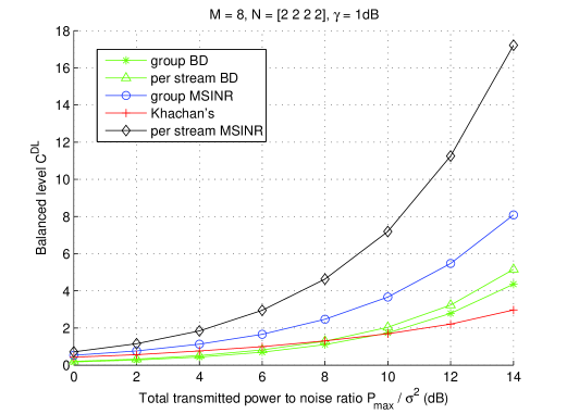
Figure 2: Comparison with [5] and BD for Problem Pr. $K=4$, $M=8$, $N_{k}=2,\;\forall k$.

Fig. 2 shows the simulation results of the balanced level ${C}^{\rm DL}$ versus total power $P_{\rm max}$ for Problem Pr, where ${C}^{\rm DL}$ is defined as in Proposition 1. The two proposed algorithms in Table II and Table V are compared with the method proposed in [5] and BD. Note that in [5], the data streams are processed separately and the balanced levels are the same for all streams. With a common SINR constraint $\gamma$ to be satisfied by all streams, the per-stream balanced level defined in [5] gives the same value as the balanced level ${C}^{\rm DL}$ defined in Proposition 1. So the comparison of ${C}^{\rm DL}$ is fair in Fig. 2. The simulation parameters are: $K=4$ users, $M=8$ transmit antennas, each user has 2 receive antennas and 2 streams ($N_{k}=L_{k}=2,\;\forall k$), and the SINR constraint $\gamma=1$. For each channel realization, all the three algorithms run until convergence but for at most 50 iterations. For fair comparison, only the cases where all the three algorithms have converged within 50 iterations are considered in averaging the performance. We will discuss the convergence probabilities later. It can be seen that the proposed group power allocation achieves higher balanced levels than the method in [5] at the positive SINR region. The proposed per stream power allocation further outperforms group power allocation. Similarly, the per stream BD achieves higher balanced levels than the group BD since the group BD is a special case of the per stream BD. Note that the BD schemes perform better when the total available power $P_{\max}$ is high and perform worse when the available power is low, since BD is a zero-forcing method which suffers from the noise enhancement problem at low $P_{\max}$. When extremely large power is available, BD will perform close to the proposed methods. However, the operating region where this phenomenon is obvious needs a much higher power than our setting in Fig. 2. We do not show the simulation results in this region since it is less practical.

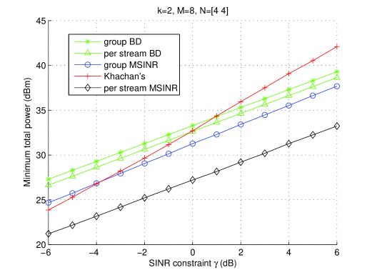
Figure 3: Comparison with [5] and BD for Problem Pp. $K=2$, $M=8$, $N_{k}=4,\;\forall k$.

In Fig. 3, we plot the minimum total required power $P_{\rm min}$ versus SINR constraint $\gamma$ for Problem Pp. Simulation parameters are $K=2$ users, $M=8$ transmit antennas, and each user has $N_{k}=4$ receive antennas and $L_{k}=4$ streams. Again, for the method in [5], a common SINR target $\gamma$ has to be achieved by all streams. Thus it has the same average SINR target $\gamma$ for each user as the other algorithms. For each channel realization, all algorithms first perform feasibility test using a large $P_{\rm max}=43$ dBm. Feasibility test for the method in [5] can be done similarly as the proposed algorithms. As soon as the feasibility test passes, the corresponding algorithm switches to the power minimization steps and runs until convergence but for at most 50 iterations. Feasibility test for BD can be done trivially. Only the cases where all the algorithms have passed the feasibility test, and converged within 50 iterations, are considered in averaging the performance. Again, we will defer the discussions for the infeasible cases and the convergence issues later. As shown in the figure, the proposed group power allocation performs better than the method in [5] at high SINR. However, at low SINR it requires more power. This is because group power allocation suffers for the fact that it cannot adjust the power within a group as the method in [5]. At low SINR, the interference is larger and the method in [5] can adjust the power within a group to better deal with the interference. On the other hand, the proposed per stream power allocation performs better than the other algorithms at both high and low SINR. Similar to Fig. 2, the BD methods perform better than the method in [5] at high SINR, but are worse than the proposed methods in all cases presented. The results at extremely high power, where the performances of BD and the proposed methods are close, are not shown due to the same reason discussed before.

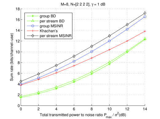
Figure 4: Sum rate comparison with [5] and BD for Problem Pr. $K=4$, $M=8$, $N_{k}=2,\;\forall k$.

We also present the sum rate comparison in Fig. 4 where the balanced levels of all users are the same (as in Fig. 2) as an indication of the QoS guaranteed and the fairness achieved. The simulation parameters are the same as in Fig. 2. Note that the sum rates of both BD methods are worse than the method in [5], while their balanced levels cross over that of [5] in Fig. 2. This is because under the same average SINR, the method in [5] will make all streams of a user have equal SINR and achieve the highest sum rate due to the concavity of the $\log$ function. Thus when a scheme’s balanced level advantage over the method in [5] is not significant enough (e.g., the BD schemes), its sum rate may be lower than that of [5]. We emphasis again that our algorithms focus on the QoS (average SINR) of individual users. Our problem formulations are fundamentally different from those focusing on sum rate optimization and not guaranteeing the QoS.

Now we show the feasibility and convergence properties of the proposed algorithms. In the above simulation setting, the number of transmit antennas $M$ is equal to the total number of data streams of all users $\sum^{K}_{k=1}L_{k}$ (also equal to the total number of receive antennas $\sum^{K}_{k=1}N_{k}$). We further consider the cases where $M<\sum^{K}_{k=1}L_{k}$ by increasing the number of users $K$. That is, for Problem Pp, $K=3$, $M=8$, and $N_{k}=L_{k}=4,\forall k;$ while for Problem Pr, $K=5$, $M=8$, $N_{k}=L_{k}=2,\forall k$. We name these cases as Case 2 and the settings for Fig. 2 and 3 as Case 1. Note that typically the system will perform scheduling [21] when $M<\sum^{K}_{k=1}L_{k}$, that is, it uses time-division multiple access (TDMA) to schedule a number of users such that $M=\sum^{K}_{k=1}L_{k}$ each time. Thus the simulation results of Case 1 represent the performance of fully loaded systems and those of Case 2 well represent the performance of over-loaded systems.

First we discuss the feasibility issues. From the simulations of Case 1, we observed that the proposed algorithms and the method in [5] passed the feasibility test for almost all channel realizations. Intuitively, group power allocation is more feasible than the method in [5] because the average, instead of per stream, SINR constraints are easier to be achieved, and they make Equation (27) better conditioned than the corresponding equation in [5]. Thus nonnegative solutions of (27) are easier to be found. In addition, since the group power allocation is a special case of the per stream power allocation with equal power distribution among the streams of a user, the per stream power allocation method should be even more feasible. As an example, when a high target SINR ($\gamma=12$ dB) is desired, simulation shows that the probabilities of feasibility for the group power allocation, the per stream power allocation, the method in [5], group BD and per stream BD are 99%, 100%, 67%, 100%, and 100%, respectively. For Case 2, the system can only support lower target SINR and the probabilities of feasibility for the above five algorithms when $\gamma=3$ dB are 100%, 100%, 0%, 0%, and 0%, respectively. Note that for Case 2, the BD based methods can not be applied since $M$ is not large enough.

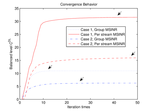
Figure 5: Convergence behaviors of the proposed algorithms for Problem Pr in Case 1 (fully loaded) and Case 2 (over loaded). The arrows point at the numbers of iterations where the algorithms meet the convergence criteria.

As for the insights to the convergence behavior, typically each optimization step improves its objective function as outlined in Section II-D. The beamforming step maximizes each user’s sum SINR of the data streams and the power allocation step optimizes the balanced level. As an example, in Fig. 5, we plot the balanced levels versus iteration times of the two proposed algorithms for Problem Pr under the same channel conditions. The total power constraint is set to 15 dBm, and the SINR constraint $\gamma=1$. The arrows point at the numbers of iterations where the algorithms meet the convergence criteria. From the figure, the two proposed algorithms typically do not oscillate often and exhibit smooth transient behaviors. We also observe that the convergence behavior of the group power allocation is slightly better than that of the per stream power allocation, i.e., the per stream power allocation is not as smooth as the group power allocation and needs more iterations to approach the balanced level. The reason why the per stream power allocation has worse convergence behavior is that after a power allocation step, the noise whitening property obtained by the previous maximum SINR filter bank may no longer be valid, that is, ${{\bf{V}}_{k}^{H}{\bf{R}}_{n,k}^{{\rm{DL}}}{\bf{V}}_{k}}$ may no longer be a scaled identity matrix. This effect may decrease the balanced level. However, in most cases this negative effect has a small impact on the eventual performance. Table VII lists the iteration times needed to converge for both problems. From these results, we can see that all three methods need more iterations to converge in Case 2. Note that for Problem Pp, the target SINRs $\gamma$ for Case 2 are smaller than those of Case 1 since the method in [5] is not feasible for $\gamma\geq 3$ dB. Also, the method in [5] needs significantly more iterations when $\gamma=2$ dB.

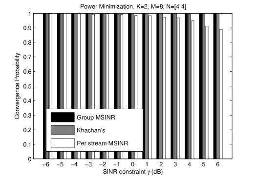
Figure 6: Comparison of the convergence probabilities for Problem Pp in Case 1 (fully loaded): $K=2$, $M=8$, $N_{k}=4,\;\forall k$.

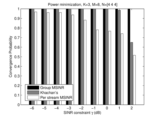
Figure 7: Comparison of the convergence probabilities for Problem Pp in Case 2 (over loaded): $K=3$, $M=8$, $N_{k}=4,\;\forall k$.

Fig. 6 shows the probabilities of the proposed algorithms and the method in [5] converging within 50 iterations given that they have passed the feasibility test, for the power minimization problem in Case 1 (settings of Fig. 3). We can see that the group power allocation and the method in [5] both exhibit good convergence probabilities while the per stream power allocation converges better at low SINR than at high SINR. The reason for the lower convergence probability of the per stream power allocation is that the linear programming makes the algorithm prone to oscillation between feasible solutions from iteration to iteration. In practice, as long as the solution is a nonnegative power vector, the SINR constraints are achieved, no matter the algorithm oscillates or not. Moreover, even when the per stream power allocation oscillates at the final iterations, typically the SINRs are still higher than that of the group power allocation. So one can simply pick the solution at the final iteration and still obtain a better performance. The other way is to avoid oscillation by switching to the group power allocation whenever the per stream power allocation algorithm oscillates. The performance of this combined algorithm should be between the performance of the per stream power allocation and the group power allocation. Fig. 7 shows the convergence probability for Problem Pp in Case 2. Since the method in [5] is not feasible when SINR constraint for $\gamma\geq 3$ dB, we only plot for $\gamma<3$ dB. The group power allocation still converges almost surely in this overloaded case.

VI Computational Complexity

In Table VI, we compare the computational complexity in one iteration based on the number of complex multiplications. From this table, one can see that there is no single step which dominates the complexity for each algorithm, so we list all of them for comparison. For each optimization step, the complexity of group power allocation (Table II) or power minimization (Table III) is lower than that of the method in [5], and we have shown in Section V that the performances of the proposed methods are also superior. The reason for the complexity saving of the group power allocation method is due to the fact that the method in [5] processes the streams separately (matrix dimension $L$), while the group power allocation processes the streams of a user jointly (matrix dimension $K$, $K<L$). For the per stream algorithms (Table V and IV), the complexity of power allocation is at most slightly higher than that of the method in [5], but the performance is much better.

In addition to the computational complexity in one iteration, the average number of iterations needed for convergence also affects the system complexity. The average numbers of iterations for the three algorithms in the simulation settings of Fig. 3 and Fig. 2 are shown in Table VII (for the power minimization Problem Pp, the average number of iterations needed by the feasibility test is included). This table shows that the group power allocation method has the fastest convergence among the three algorithms, while the per stream power allocation has the slowest convergence. Compared to the method in [5], the group power allocation has a lower computational complexity, converges faster and performs better. If more complicated computation is allowed, the per stream power allocation exhibits even better performance.

As for the BD algorithms used in this paper, the computation of the zero-forcing transmit beamformers has approximately the same complexity as that of the “uplink beamforming” step of Group (Pr) in Table VI; while the complexity for receiver beamformers is approximately the same as that of “downlink beamforming” step of Group (Pr). The complexity of the power allocation steps is negligible compared with those of the beamformers. Since the BD algorithms do not need iterations, they are not listed in the comparisons in Tables VI and VII (nor in Fig. 6).

VII Conclusion

Efficient solutions to the joint transmit-receive beamforming and power allocation under average SINR constraints in the multi-user MIMO downlink systems were proposed. The beamforming filter is a GSINR-FB which exploits the intra-group cooperation of grouped data streams. Due to this selection, the SINR balancing structure of optimal power allocation holds and simplifies the computation. Based on the uplink-downlink duality, we formulated the dual problem in the virtual uplink, and iteratively solved the optimal beamforming filters and power allocation matrices. The proposed algorithms are generalizations of the one in [4] to the scenario with multiple receive antennas per user, and exploit the receiver diversity more effectively than [5]. Simulation results demonstrated the superiority of the proposed algorithms over methods based on independent data stream processing [5] and BD in terms of performance. Moreover, the computational complexities of the proposed methods are comparable with that of [5].

TABLE I: Basic Steps of the $n$th Iteration

1:	First Downlink Power Allocation
	Fixed ${\bf U}^{(n)}$ and ${\bf V}^{(n)}$, find new ${\bf P}^{(2n+1)}$
2:	Downlink Receive Maximum SINR Beamforming
	Fixed ${\bf P}^{(2n+1)}$ and ${\bf U}^{(n)}$, find new ${\bf V}^{(n+1)}$
3:	Second Downlink Power Allocation
	Fixed ${\bf U}^{(n)}$ and ${\bf V}^{(n+1)}$, find new ${\bf P}^{(2n+2)}$
4:	First Virtual Uplink Power Allocation
	Fixed ${\bf V}^{(n+1)}$ and ${\bf U}^{(n)}$, find new ${\bf Q}^{(2n+1)}$
5:	Virtual Uplink Receive Maximum SINR Beamforming
	Fixed ${\bf Q}^{(2n+1)}$ and ${\bf V}^{(n+1)}$, find new ${\bf U}^{(n+1)}$
6:	Second Virtual Uplink Power Allocation
	Fixed ${\bf U}^{(n+1)}$ and ${\bf V}^{(n+1)}$, find new ${\bf Q}^{(2n+2)}$.

TABLE II: Iterative algorithm for Problem Pr with group power allocation

Initialization: $\mathbf{U}=\mathbf{I},\mathbf{V}=\mathbf{I}$
Iteration:
1:	First Downlink Power Allocation with Sum Power Constraint
	Solve $\bf p$ in $\mathbf{\Upsilon}\begin{pmatrix}\mathbf{p}\\ 1\end{pmatrix}=\frac{1}{{C^{{\rm{DL}}}}}\begin{pmatrix}\mathbf{p}\\ 1\end{pmatrix}$
2:	Downlink Receive Maximum SINR Beamforming
	for $k=1:K$
	$\mathbf{V}_{k}=eig(\mathbf{R}_{s,k}^{\mathrm{DL}},\mathbf{R}_{n,k}^{\mathrm{DL}})$
3:	Second Downlink Power Allocation with Sum Power Constraint
	Solve $\bf p$ in $\mathbf{\Upsilon}\begin{pmatrix}\mathbf{p}\\ 1\end{pmatrix}=\frac{1}{{C^{{\rm{DL}}}}}\begin{pmatrix}\mathbf{p}\\ 1\end{pmatrix}$
4:	First Virtual Uplink Power Allocation with Sum Power Constraint
	Solve $\bf q$ in $\mathbf{\Lambda}\begin{pmatrix}\mathbf{q}\\ 1\end{pmatrix}=\frac{1}{{C^{{\rm{UL}}}}}\begin{pmatrix}\mathbf{q}\\ 1\end{pmatrix}$
5:	Virtual Uplink Receive Maximum SINR Beamforming
	for $k=1:K$
	$\mathbf{U}_{k}=eig(\mathbf{R}_{s,k}^{\mathrm{UL}},\mathbf{R}_{n,k}^{\mathrm{UL}})$
6:	Second Virtual Uplink Power Allocation with Sum Power Constraint
	Solve $\bf q$ in $\mathbf{\Lambda}\begin{pmatrix}\mathbf{q}\\ 1\end{pmatrix}=\frac{1}{{C^{{\rm{UL}}}}}\begin{pmatrix}\mathbf{q}\\ 1\end{pmatrix}$
7:	Repeat steps 1-6 until convergence, i.e., $|C^{{\rm DL}(n)}-C^{{\rm DL}(n-1)}|<\epsilon$

TABLE III: Iterative algorithm for Problem Pp with group power allocation

Initialization: Feasibility test using the algorithm in Table II   , if failure then exit.
Iteration:
1:	First Downlink Power Minimization
	${\bf{p}}=({\bf{I}}-{\bf{D\Psi}})^{-1}{\bf{D\bm{\sigma}}}$
2:	Downlink Receive Maximum SINR Beamforming
	for $k=1:K$
	$\mathbf{V}_{k}=eig(\mathbf{R}_{s,k}^{\mathrm{DL}},\mathbf{R}_{n,k}^{\mathrm{DL}})$
3:	Second Downlink Power Minimization
	${\bf{p}}=({\bf{I}}-{\bf{D\Psi}})^{-1}{\bf{D\bm{\sigma}}}$
4:	First Virtual Uplink Power Minimization
	${\bf{q}}=({\bf{I}}-{\bf{D\Psi}}^{T})^{-1}{\bf{D\bm{\sigma}}}$
5:	Virtual Uplink Receive Maximum SINR Beamforming
	for $k=1:K$
	$\mathbf{U}_{k}=eig(\mathbf{R}_{s,k}^{\mathrm{UL}},\mathbf{R}_{n,k}^{\mathrm{UL}})$
6:	Second Virtual Uplink Power Minimization
	${\bf{q}}=({\bf{I}}-{\bf{D\Psi}}^{T})^{-1}{\bf{D\bm{\sigma}}}$
7:	Repeat steps 1-6 until convergence, i.e., $|C^{{\rm DL}}-1|<\epsilon$

TABLE IV: Iterative algorithm for Problem Pp with per stream power allocation

Initialization: Feasibility test using the algorithm in Table V   , if failure then exit.
Iteration:
1:	First Downlink Power Minimization
	Solve $\bf p$ in the linear programming problem:
	$\begin{array}[]{l}\min{\rm{\ }}{\bf{1}}^{T}{\bf{p}}\\ {\rm{s.t.\ \ }}\sum\limits_{l=1}^{L_{k}}{p_{kl}[{\bf{A}}_{kk}]_{ll}/\gamma_{k}}-\sum\limits_{j=1,j\neq k}^{K}{\sum\limits_{l=1}^{L_{j}}{p_{jl}[{\bf{A}}_{jk}]_{ll}}}=L_{k}\sigma^{2},\\ \hskip 19.91692pt{\rm{for\ }}k=1,...,K,{\rm{\ and\ }}\mathbf{p}\geq_{e}0\\ \end{array}$
2:	Downlink Receive Maximum SINR Beamforming
	for $k=1:K$
	$\mathbf{V}_{k}=eig(\mathbf{R}_{s,k}^{\mathrm{DL}},\mathbf{R}_{n,k}^{\mathrm{DL}})$
3:	Second Downlink Power Minimization
	Solve $\bf p$ in the linear programming problem:
	$\begin{array}[]{l}\min{\rm{\ }}{\bf{1}}^{T}{\bf{p}}\\ {\rm{s.t.\ \ }}\sum\limits_{l=1}^{L_{k}}{p_{kl}[{\bf{A}}_{kk}]_{ll}/\gamma_{k}}-\sum\limits_{j=1,j\neq k}^{K}{\sum\limits_{l=1}^{L_{j}}{p_{jl}[{\bf{a}}_{jk}]_{ll}}}=L_{k}\sigma^{2},\\ \hskip 19.91692pt{\rm{for\ }}k=1,...,K,{\rm{\ and\ }}\mathbf{p}\geq_{e}0\\ \end{array}$
4:	First Virtual Uplink Power Minimization
	Solve $\bf q$ in the linear programming problem:
	$\begin{array}[]{l}\min{\rm{\ }}{\bf{1}}^{T}\mathbf{q}\\ {\rm{s.t.\ \ }}\sum\limits_{l=1}^{L_{k}}{q_{kl}[{\bf{B}}_{kk}]_{ll}/\gamma_{k}}-\sum\limits_{j=1,j\neq k}^{K}{\sum\limits_{l=1}^{L_{j}}{q_{jl}[{\bf{B}}_{kj}]_{ll}}}=L_{k}\sigma^{2},\\ \hskip 19.91692pt{\rm{for\ }}k=1,...,K,{\rm{\ and\ }}\mathbf{q}\geq_{e}0\\ \end{array}$
5:	Virtual Uplink Receive Maximum SINR Beamforming
	for $k=1:K$
	$\mathbf{U}_{k}=eig(\mathbf{R}_{s,k}^{\mathrm{UL}},\mathbf{R}_{n,k}^{\mathrm{UL}})$
6:	Second Virtual Uplink Power Minimization
	Solve $\bf q$ in the linear programming problem:
	$\begin{array}[]{l}\min{\rm{\ }}{\bf{1}}^{T}\mathbf{q}\\ {\rm{s.t.\ \ }}\sum\limits_{l=1}^{L_{k}}{q_{kl}[{\bf{B}}_{kk}]_{ll}/\gamma_{k}}-\sum\limits_{j=1,j\neq k}^{K}{\sum\limits_{l=1}^{L_{j}}{q_{jl}[{\bf{B}}_{kj}]_{ll}}}=L_{k}\sigma^{2},\\ \hskip 19.91692pt{\rm{for\ }}k=1,...,K,{\rm{\ and\ }}\mathbf{q}\geq_{e}0\\ \end{array}$
7:	Repeat steps 1-6 until convergence, i.e., $|C^{{\rm DL}}-1|<\epsilon$

TABLE V: Iterative algorithm for Problem Pr with per stream power allocation

Initialization: $\mathbf{U}=\mathbf{I},\mathbf{V}=\mathbf{I}$
Iteration:
1:	First Downlink Power Allocation with Sum Power Constraint
	$t_{k}^{(2n+1)}=\frac{{P_{\max}}}{{G_{k}^{(2n)}\sum\limits_{j=1}^{K}{\frac{1}{{G_{j}^{(2n)}}}}}}$, where $G_{k}^{(2n)}=\frac{{g_{kk}/\gamma_{k}}}{{\sum\limits_{j\neq k}{t_{j}^{(2n)}g_{jk}}+L_{k}\sigma^{2}}}$.
2:	Downlink Receive Maximum SINR Beamforming
	for $k=1:K$
	$\mathbf{V}_{k}=eig(\mathbf{R}_{s,k}^{\mathrm{DL}},\mathbf{R}_{n,k}^{\mathrm{DL}})$
3:	Second Downlink Power Allocation with Sum Power Constraint
	$t_{k}^{(2n+2)}=\frac{{P_{\max}}}{{G_{k}^{(2n+1)}\sum\limits_{j=1}^{K}{\frac{1}{{G_{j}^{(2n+1)}}}}}}$, where $G_{k}^{(2n+1)}=\frac{{g_{kk}/\gamma_{k}}}{{\sum\limits_{j\neq k}{t_{j}^{(2n+1)}g_{jk}}+L_{k}\sigma^{2}}}$.
4:	First Virtual Uplink Power Allocation with Sum Power Constraint
	$s_{k}^{(2n+1)}=\frac{{P_{\max}}}{{H_{k}^{(2n)}\sum\limits_{j=1}^{K}{\frac{1}{{H_{j}^{(2n)}}}}}}$, where $H_{k}^{(2n)}=\frac{{h_{kk}/\gamma_{k}}}{{\sum\limits_{j\neq k}{s_{j}^{(2n)}h_{jk}}+L_{k}\sigma^{2}}}$.
5:	Virtual Uplink Receive Maximum SINR Beamforming
	for $k=1:K$
	$\mathbf{U}_{k}=eig(\mathbf{R}_{s,k}^{\mathrm{UL}},\mathbf{R}_{n,k}^{\mathrm{UL}})$
6:	Second Virtual Uplink Power Allocation with Sum Power Constraint
	$s_{k}^{(2n+2)}=\frac{{P_{\max}}}{{H_{k}^{(2n+1)}\sum\limits_{j=1}^{K}{\frac{1}{{H_{j}^{(2n+1)}}}}}}$, where $H_{k}^{(2n+1)}=\frac{{h_{kk}/\gamma_{k}}}{{\sum\limits_{j\neq k}{s_{j}^{(2n+1)}h_{jk}}+L_{k}\sigma^{2}}}$.
7:	Repeat steps 1-6 until convergence, i.e., $|C^{{\rm DL}(n)}-C^{{\rm DL}(n-1)}|<\epsilon$

TABLE VI: Complexities of the optimization steps in one iteration

	Uplink Beamforming	Uplink Power Allocation	Downlink Beamforming	Downlink Power Allocation
Group (Pr)	$O(KM^{3})$	$O((K+1)^{3})$	$O(\sum_{k=1}^{K}L_{k}^{3})$	$O((K+1)^{3})$
Group (Pp)	$O(KM^{3})$	$O(K^{3})$	$O(\sum_{k=1}^{K}L_{k}^{3})$	$O(K^{3})$
Per Stream (Pr)	$O(KM^{3})$	$O(\sum_{k=1}^{K}L_{k}^{2}M)$	$O(\sum_{k=1}^{K}L_{k}^{3})$	$O(\sum_{k=1}^{K}L_{k}^{2}M)$
Per Stream (Pp)	$O(KM^{3})$	$O(L^{3.5})$	$O(\sum_{k=1}^{K}L_{k}^{3})$	$O(L^{3.5})$
Khachan’s (Pr)	$O(LM^{3})$	$O(L^{3})$	$O(\sum_{k=1}^{K}L_{k}^{4})$	$O(L^{3})$
Khachan’s (Pp)	$O(LM^{3})$	$O(L^{3})$	$O(\sum_{k=1}^{K}L_{k}^{4})$	$O(L^{3})$

TABLE VII: Average numbers of iterations needed for convergence

Case 1 (Fully loaded)
Problem Pp					Problem Pr
SINR constraint ($\gamma$)	2	4	6		Pmax(dB)	10	12	14
Group	9.6500	10.7200	11.7200			12.359	12.608	12.558
Khachan’s	15.3720	17.7600	21.7200			13.857	13.316	13.382
Per Stream	25.7861	26.1097	30.2598			15.475	14.871	13.906
Case 2 (Over loaded)
Problem Pp					Problem Pr
SINR constraint ($\gamma$)	-2	0	2		Pmax(dB)	10	12	14
Group	10.41	11.88	14.96			15.43	17.37	20.31
Khachan’s	16.63	22.97	40.93			14.11	14.58	15.72
Per Stream	25.78	26.10	30.25			17.53	18.3	17.04

References

- [1] F. Rashid-Farrokhi, K. J. R. Liu, and L. Tassiulas, “Transmit beamforming and power control for cellular wireless systems,” IEEE J. Select. Areas Commun., vol. 16, no. 8, pp. 1437–1450, 1998.
- [2] A. Bourdoux and N. Khaled, “Joint Tx-Rx optimisation for MIMO-SDMA based on a null-space constraint,” in Proc. of IEEE Vehicular Technology Conference (VTC-02 Fall), Sep. 2002, pp. 171–174.
- [3] L.-U. Choi and R. D. Murch, “A transmit preprocessing technique for multiuser MIMO systems using a decomposition approach,” IEEE Trans. Wireless Commun., vol. 3, no. 1, pp. 2–24, Jan. 2004.
- [4] M. Schubert and H. Boche, “Solution of the multiuser downlink beamforming problem with individual SINR constraints,” IEEE Trans. Veh. Technol., vol. 53, no. 1, pp. 18–28, Jan. 2004.
- [5] A. Khachan, A. Tenenbaum, and R. S. Adve, “Linear processing for the downlink in multiuser MIMO systems with multiple data streams,” in IEEE International Conf. on Communications, Jun. 2006.
- [6] H.-J. Su and E. Geraniotis, “Maximum signal-to-noise array processing for space-time coded systems,” IEEE Trans. Commun., vol. 50, no. 8, pp. 1419–1422, Sep. 2002.
- [7] J. Wang and D. P. Palomar, “Worst-case robust MIMO transmission with imperfect channel knowledge,” IEEE Trans. Signal Processing, pp. 3086–3100, Aug. 2009.
- [8] A. Abdel-Samad, T. Davidson, and A. Gershman, “Robust transmit eigen beamforming based on imperfect channel state information,” IEEE Trans. Signal Processing, vol. 54, no. 5, pp. 1596–1609, 2006.
- [9] D. Tse and P. Viswanath, “Downlink-uplink duality and effective bandwidths,” in Proc. IEEE Int. Symp. Inf. Theory (ISIT), Jul. 2002.
- [10] H. Boche and M. Schubert, “Optimal multi-user interference balancing using transmit beamforming,” in Wireless Personal Comm. (WPC), 2003.
- [11] M. Schubert and H. Boche, “A unifying theory for uplink and downlink multi-user beamforming,” in Proc. IEEE Intern. Zurich Seminar, Jul. 2002.
- [12] N. Jindal, S. Vishwanath, and A. Goldsmith, “On the duality of Gaussian multiple-access and broadcast channels,” IEEE Trans. Inform. Theory, vol. 50, no. 5, pp. 768–783, May 2004.
- [13] G. Caire, N. Jindal, M. Kobayashi, and N. Ravindran, “Multiuser MIMO Achievable Rates with Downlink Training and Channel State Feedback,” IEEE Trans. Inform. Theory, vol. 56, no. 6, pp. 2845–2866, June. 2010.
- [14] M. Biguesh and A. Gershman, “Training-based MIMO channel estimation: a study of estimator tradeoffs and optimal training signals,” IEEE Trans. Signal Processing, vol. 54, no. 3, pp. 884–893, Aug. 2006.
- [15] S. Haykin, Communication Systems, 4th ed. John Wiley Sons, Inc., 2001.
- [16] J. Proakis, Digital communications, 4th ed. McGraw-hill, 2000.
- [17] R. Horn and C. Johnson, Matrix Analysis. Cambridge University Press, 1990.
- [18] W. Yang and G. Xu, “Optimal downlink power assignment for smart antenna systems,” in Proc. IEEE Int. Conf. Acoust., Speech, and Signal Proc. (ICASSP), May 1998.
- [19] S. Boyd and L. Vandenberghe, Convex Optimization. Cambridge University Press, 2003.
- [20] N. Jindal, W. Rhee, S. Vishwanath, and S. A. Jafar, “Sum power iterative water-filling for multi-antenna Gaussian broadcast channels,” IEEE Trans. Inform. Theory, vol. 51, no. 4, pp. 1570– 1580, Apr. 2005.
- [21] D. Tse and P. Viswanath, Fundamentals of Wireless Communication. Cambridge University Press, 2005.