Random Access Game in Fading Channels with Capture: Equilibria and Braess-like Paradoxes

Abstract

The Nash equilibrium point of the transmission probabilities in a slotted ALOHA system with selfish nodes is analyzed. The system consists of a finite number of heterogeneous nodes, each trying to minimize its average transmission probability (or power investment) selfishly while meeting its average throughput demand over the shared wireless channel to a common base station (BS). We use a game-theoretic approach to analyze the network under two reception models: one is called power capture, the other is called signal to interference plus noise ratio (SINR) capture. It is shown that, in some situations, Braess-like paradoxes may occur. That is, the performance of the system may become worse instead of better when channel state information (CSI) is available at the selfish nodes. In particular, for homogeneous nodes, we analytically presented that Braess-like paradoxes occur in the power capture model, and in the SINR capture model with the capture ratio larger than one and the noise to signal ratio sufficiently small.

EDICS     SPC-BBND,  SPC-PERF

I Introduction

The simplicity of ALOHA [1] and slotted ALOHA [2] systems proposed in the 1970s for random access have attracted a large amount of research. From the system perspective, the earlier works focused on the issues of average throughput and stability of ALOHA systems with homogeneous users. That is, these works usually assumed that all users in the network have the same statistical characteristics, thus only considered the macroscopic (or network-wide average) performance. The readers are referred to [3] and the references therein for the analyses of slotted ALOHA in fading channels with capture.

Recently, MacKenzie and Wicker [4] first considered slotted ALOHA from the user perspective. They assumed that there is no centralized scheduling, and each user acts selfishly to maximize its own utility function. They then analyzed the Nash equilibrium point by game theory [5]. Game theory is a useful tool for modeling and studying the interaction of strategic interactions among selfish players. The most important equilibrium concept in game theory is the Nash equilibrium (named after its inventor John Nash) at which there is no incentive for any player to unilaterally deviate. The selfish ALOHA system is more robust and scalable for implementation than a system with centralized control.

The analysis of [4] was extended in [6] to the case with heterogenous users whose costs of transmission are not identical. The behavior of the network throughput at the Nash equilibria as a function of the costs was analyzed. Unfortunately, the cost is not a parameter one can easily control. It is determined by the relative cost of transmission as compared to the value of a success.

Incorporating the availability of CSI into an ALOHA system, [12] investigated the Nash equilibrium points of CSI-dependent transmission probabilities for heterogenous nodes in time-varying channels. In that channel-aware ALOHA system, each node tries to minimize its average transmission probability selfishly while meeting its average throughput demand to the common base station (BS). It was shown that the feasible region of the nodes’ throughput demands in the selfish ALOHA is equivalent to the achievable region by a system with centralized control. Moreover, within the feasible region, exactly two Nash equilibrium points exist. This work considerably extended the analysis of the network model by Jin and Kesidis [11].

Other related works on CSI-dependent transmission probabilities in channel-aware ALOHA networks include [13][14][15]. In [13], the analysis of [12] under the collision model was extended to the capture model in static channels. It was shown that while multiple Nash equilibria may exist, one of them is uniformly preferable in the sense of minimum transmission probability. In [14], the authors considered the network model in [12] without the backlogged assumption, and found that, different from [12], infinitely many equilibrium points may exist with the distributed algorithm if the slotted ALOHA is stable. A slotted ALOHA system with general multipacket reception (MPR) [16][17] was considered in [15]. It was shown that, for selfish nodes to maximize their individual utilities (including transmission and waiting costs), the structure of CSI-dependent transmission probabilities is a threshold strategy.

The availability of CSI was used to vary transmission power rather than transmission probability in [18]. The authors of [18] derived an explicit CSI-dependent power allocation strategy at the Nash equilibrium point in a slotted ALOHA system with capture, under the assumption that channel gain is uniformly distributed. It was shown that as the number of nodes increases, the system performance with the power allocation strategy at the symmetric Nash equilibrium point approaches that with the optimal mandated power allocation strategy.

In [19], not only CSI-dependent transmission probabilities but also CSI-dependent transmission power levels were considered. Through numerical study, it was shown that the additional allowance of CSI-dependent transmission power levels may make the system performance worse instead of better as compared to that with only the CSI-dependent transmission probabilities [12]. This kind of counterintuitive phenomena, which demonstrate a performance degradation when more information or resource is added to a noncooperative network, is known as the Braess paradox, introduced by Braess in transportation network planning [10]. There are other Braess-like paradoxes discovered in different contexts, for example, in the contexts of queueing network [21], computer network [22][23][24][25], and wireless communication [26].

The game-theoretic approach has widely been applied in communication networks. For example, MacKenzie and Wicker [7] showed that game theory can be applied to developing self-configuring wireless networks. Cui, Chen and Low [8] showed a game-theoretic framework for contention-based medium access control. Lee et al. [9] revealed the noncooperative nature of random access from MAC reverse-engineering. They discovered that, in the current backoff-based MAC protocol, the users are participating implicitly in a noncooperative game.

In this paper, we also consider the network model in [12]. Our work analyzes the Nash equilibrium point of transmission probabilities in fading channels under two more general capture models both including the collision model [12] as a special case. We also extend the analysis of [13] for static channels to fading channels. The main contribution of our work that differentiates it from the earlier works studying the CSI-dependent transmission probability in selfish ALOHA [12][13][15] is that we find that Braess-like paradoxes may occur under some situations. In other words, in some situations, the availability of CSI may degrade the performance (in terms of, e.g., total power consumption, throughput, etc.). We call this phenomenon a Braess-like paradox due to its analogy to the Braess paradox. To the best of our knowledge, our work is the first to show a Braess-like paradox analytically in a random access network, and this paradox does not occur in the collision model considered in [12]. Such a discovery is important because it was generally believed that the additional availability of CSI should improve, at least not degrade, the network performance.

The two capture models we consider in this paper are similar to the capture model in [20] for static channels. Specifically, one model is called the signal to interference plus noise ratio (SINR) capture model in which the BS receives the packet of a node successfully if the node’s SINR is larger than the capture ratio $b$. When $b<1$, it is possible for the BS to successfully receive more than one node’s packets as in, for example, CDMA systems whose signal quality can be highly increased after despreading. When $b>1$, at most one node’s packet is successfully received as in typical narrowband systems which need the SINR to be high enough to operate properly. The other model is called the power capture model in which the BS receives the packet of a node successfully if the node has the strongest received power which is at least $1+\Delta$ times stronger than the received power of every other node, where $\Delta\geq 0$ models a guard zone to counter interference.

Our work also reveals that when CSI is not available to selfish nodes, any achievable throughput demands in the SINR capture model can be achieved by a Nash equilibrium point with its sum of the transmission probabilities of different nodes no larger than a constant which depends only on the capture ratio. As for the power capture model, our analysis shows that when CSI is not available to selfish nodes and $\Delta=0$ or when perfect CSI is available to selfish nodes and $\Delta\leq\frac{1}{n-1}$, where $n$ is the number of nodes in the network, there exists a unique Nash equilibrium point for any achievable throughput demands. When $\Delta=\infty$, the number of Nash equilibrium points becomes exactly two.

The remainder of the paper is organized as follows. We formulate our random access game in Section II. The analysis of the Nash equilibrium points and the discussion of Braess-like paradoxes are given under the SINR capture model in Section III and under the power capture model in Section IV. In Section V, we provide one distributed mechanism which can make the system converge to the Nash equilibrium. The paper is then concluded in Section VI.

II Problem Formulation

We consider a wireless network where $n$ nodes transmit at the same fixed power level $P_{T}$ to a BS over a shared channel. Time is slotted, and each transmission attempt sends a packet which occupies one time slot. The amount of information contained in a packet is fixed and is the same for all nodes. Thus, for the brevity of analysis, the throughput is defined in terms of the average number of successfully received packets (which is commonly used under the capture or MPR model, e.g., [27]). All nodes are synchronized so that each transmission attempt starts at the slot boundary.

At time slot $k$, the signal $y_{k}$ received by the BS is given by

$$y_{k}=\sum^{n}_{i=1}h_{i,k}B_{i,k}d_{i,k}+\eta_{k}$$ (1)

where

$$B_{i,k}=\begin{cases}1&\text{if node $i$ transmits in time slot $k$}\\ 0&\text{otherwise}\end{cases},$$

$h_{i,k}$ is the channel gain between node $i$ and the BS, $d_{i,k}$ is the signal from node $i$ (with transmission power $P_{T}$), and $\eta_{k}$ is the additive noise at the BS.

The channel gains $h_{i,k}$ are assumed to be independent and identically distributed (i.i.d.) among all nodes, fixed within a time slot, and varying from time slot to time slot as in [12]. For clarity of the analysis, the channel gain of any particular node is assumed to be an i.i.d. process with respect to time. Note that even if the channel gain of a node is merely assumed to be a stationary and ergodic process, the results of this paper derived based on stationary strategies can be shown to hold. The readers are referred to [12, Section II] for discussion on this assumption. It is further assumed that, at the beginning of time slot $k$, node $i$ may be able to obtain its own instantaneous CSI $z_{i,k}$, which provides an indication of the quality of the current channel between that node and the BS. For a TDD system, the CSI may be measured by individual nodes based on the signal from the BS (e.g., a periodic pilot signal) and the channel reciprocity. In an FDD system, the knowledge of CSI may be obtained via feedback from the BS. Our model only assumes that some sort of instantaneous CSI is available and does not restrict how the CSI is obtained. In practice, instantaneous CSI may be difficult to derive from the feedback from the BS due to the busty nature of random access which may introduce a random time lag between the time the BS measures the CSI and the time of transmission of a node. Thus our system model is more applicable to TDD systems. Assume the number of possible values of $z_{i,k}$ is $x_{i}$, and $z_{i,k}$ belongs to the set $\{z_{i1},z_{i2},\dots,z_{ix_{i}}\}$ with $z_{i1}<z_{i2}<\cdots<z_{ix_{i}}$. Here the assumption of finite discrete (quantized) CSI is taken for convenience only, and can be relaxed. For the analysis in this paper to hold, the only required property of the mapping from the channel gain to the CSI is that a larger value of CSI corresponds to a higher range of absolute channel gain $|h_{i,k}|$. By excluding the CSI values observed with probability zero, we can assume that the probability of observing each element in the set $\{z_{i1},z_{i2},\dots,z_{ix_{i}}\}$ is larger than zero. Note that the case where CSI is not available can be seen as a special case with only one possible CSI value.

II-A Two Capture Models

1. The SINR capture model: in this model, node $i$’s packet will be successfully received at time slot $k$ if $SINR_{i,k}>b$, where $b$ is the capture ratio, and $SINR_{i,k}$ is the SINR of node $i$ at time slot $k$ given by

   $$SINR_{i,k}=\frac{B_{i,k}|h_{i,k}|^{2}P_{T}}{\sum_{j\neq{}i}B_{j,k}|h_{j,k}|^{2}P_{T}+N_{0}}$$ (2)

   with $N_{0}$ being the power of the additive noise at the BS. If we set $N_{0}=0$ and the capture ratio $b=\infty$, this capture model becomes the collision model.

2. The power capture model: in this model, node $i$’s packet is successfully received at time slot $k$ if

   $$B_{i,k}|h_{i,k}|^{2}>\max_{j\neq i}\{(1+\Delta)B_{j,k}|h_{j,k}|^{2}\},$$ (3)

   where $\Delta\geq 0$. When $\Delta=\infty$, we have the collision model; and when $\Delta=0$, we have the perfect power capture model for which the packet with the highest received power is always captured.

Throughout this paper, we will only consider that the channels are i.i.d. Rayleigh fading [28]. This is the most commonly used model in wireless communications in urban areas. Hence, $|h_{i,k}|^{2}$ are i.i.d. exponential random variables.

II-B Noncooperative Game Formulation

In the network, each node tries to minimize its average transmission probability (or equivalently, average power investment) and selfishly makes the decision whether to transmit or not according to the current CSI, while meeting the average throughput demand (in packets per slot), denoted $\rho_{i}$ for node $i$. It is further assumed that all nodes always have packets buffered for transmission at any time.

This system can be modeled as a noncooperative game with constraints which are the average throughput demands. The selfish nodes are the players, and the action of a player (node) at every time slot is to transmit or not. For generality, in order to meet any average throughput demand while minimizing the average transmission probability, the decision whether to transmit or not is relaxed from being deterministic to being probabilistic. To this end, an action is defined as transmission with a certain probability. With the i.i.d. channel gain processes, we focus on stationary transmission strategies (as in [12]) which depend on the current CSI. Thus, we let $\textbf{s}_{i}=(s_{i1},s_{i2},\ldots,s_{ix_{i}})\in{}[0,1]^{x_{i}}$ denote node $i$’s transmission strategy such that it transmits with probability $s_{im}$ (the $m$-th entry of $\textbf{s}_{i}$) when the CSI is $z_{im}$. $\{s_{i1},s_{i2},\ldots,s_{ix_{i}}\}$ also defines the action space of node $i$. Besides the actions of transmission with certain probabilities, the other action of node $i$ is to adjust its transmission strategy $\textbf{s}_{i}$ such that it can sustain the average throughput demand while minimizing the average transmission probability denoted by $p_{i}$. The Nash equilibria of the stationary transmission strategies and how the nodes can adjust their transmission strategies in this noncooperative game to arrive at an equilibrium will be discussed later.

Due to the constraints (average throughput demands), the average transmission probabilities (power investments) of the nodes are nonzero (except for the trivial case with zero throughput demand), and the interaction between nodes is through their mutual interference or competition to have the highest received power. We now discuss the best response strategies for each selfish node in the network.

Definition 1

A stationary threshold strategy for node $i$ has the form $\textbf{s}_{i}=(0,\ldots,0,s_{im},1\ldots,1)$. That is, the node always transmits when the CSI is larger than the threshold $z_{im}$, and never transmits when the CSI is smaller than $z_{im}$, while the transmission probability when the CSI is $z_{im}$ is $s_{im}$.

For example, $\textbf{s}_{i}=(0,\ldots,0,0.5,1)$ means that node $i$ always transmits when the CSI is the largest one, and transmits with probability $0.5$ when the CSI is the second largest one. For the other CSI values, node $i$ does not transmit.

We have the following proposition as in [12] that the stationary threshold strategy is the best response transmission strategy for each node. The reason is that transmitting at higher CSI will result in higher probability of packet success (or higher throughput), hence more power saving. To be more specific, since the channels of different nodes are independent, for a particular node which does not know the CSI of the other nodes, no matter at what time slot this node transmits and what the other nodes transmission strategies are, the packet success probability of this node will be affected by the other nodes through the average interferences they cause. Thus, for the node in consideration, transmitting when its CSI is higher will result in higher average SINR and hence higher success probability in the SINR capture model. With a similar argument, transmitting at higher CSI will also result in higher success probability in the power capture model. Since the proof is similar to that of [12, Lemma 1], we omit it.

Proposition 1

The best response transmission strategy for each selfish node in terms of minimizing its average transmission probability (or average power investment) while meeting the average throughput demand, is a threshold strategy under the power capture and the SINR capture models.

Remarks:

1. As a result of Proposition 1, we have that a threshold strategy $\textbf{s}_{i}=(s_{i1},s_{i2},\ldots,s_{ix_{i}})=(0,\ldots,0,s_{im},1\ldots,1)$ uniquely determines the average transmission probability $p_{i}$ of node $i$ by

   $$p_{i}=s_{im}P_{i}(m)+\sum^{x_{i}}_{j=m+1}P_{i}(j)$$ (4)

   where $P_{i}(j)$ is the probability of occurrence of $z_{ij}$ for node $i$. Therefore, we will analyze the Nash equilibrium in terms of $p_{i}$ (as in [12]) in the remainder of this paper.

2. The best response strategy for a node to adjust its average transmission probability (hence the corresponding stationary threshold strategy) in reaction to the given strategies of the other nodes, is to equalize the throughput achieved by the average transmission probability with the average throughput demand (so the average transmission probability is minimized) [12].

3. In the case when CSI is not available (equivalently, there is only one possible CSI value), the threshold strategy of node $i$ becomes random transmission with probability $p_{i}$ at every time slot. The action space in this case (with only one possible action) is apparently smaller than that of the case when CSI is available. In the limiting case when perfect CSI is available (e.g., the CSI takes the exact value of $|h_{i,k}|$ for node $i$ at time slot $k$, that is, there are an infinite number of possible CSI values), the threshold strategy of node $i$ becomes transmission only if the CSI is above the threshold which is selected such that the average transmission probability is $p_{i}$. In the sequel, only the limiting cases without CSI and with perfect CSI are considered for the brevity of analytically studying the Nash equilibrium points and presenting the Braess-like paradoxes.

II-C Nash Equilibria

Let $\textbf{p}_{-i}$ represent the vector of the transmission probabilities of all nodes except node $i$, and $r_{i}(p_{i},\textbf{p}_{-i})$ represent the average throughput of node $i$ when it transmits with probability $p_{i}$ given that the other nodes transmit with probability vector $\textbf{p}_{-i}$. For the noncooperative game in consideration, we define the transmission probability vector $\textbf{p}=(p_{1},\ldots,p_{n})\in[0,1]^{n}$ as an action profile. The utility function for node $i$, given that the other nodes transmit with probability vector $\textbf{p}_{-i}$, is defined as $U_{i}(p_{i},\textbf{p}_{-i})=1-p_{i}$ (which may be seen as the power left for node $i$).

We give the definition of the (constrained) Nash equilibrium point in our noncooperative game.

Definition 2

An action profile p is a (constrained) Nash equilibrium point if for all $i=1,\ldots,n$, we have

$$\begin{cases}r_{i}(p_{i},\textbf{p}_{-i})\geq\rho_{i}\\ U_{i}(p_{i},\textbf{p}_{-i})\geq U_{i}(\tilde{p}_{i},\textbf{p}_{-i}),~{}\forall\tilde{p}_{i}\in\{\tilde{p}_{i}:r_{i}(\tilde{p}_{i},\textbf{p}_{-i})\geq\rho_{i}\},\end{cases}$$ (5)

where $\rho_{i}$, the average throughput demand, defines a constraint.

Equivalently, p is a Nash equilibrium point if

$$p_{i}\in\arg\min_{0\leq\tilde{p}_{i}\leq 1}\{\tilde{p}_{i}:r_{i}(\tilde{p}_{i},\textbf{p}_{-i})\geq\rho_{i}\},~{}\forall\ i=1,\ldots,n.$$ (6)

The above expression means that at a Nash equilibrium point p, each node $i$ would not prefer to deviate from its choice of transmission probability. It should be noted that our problem is a noncooperative game with constraints, so there are additional constraints in defining our Nash equilibrium point that differs from the conventional Nash equilibrium point.

Since $r_{i}(p_{i},\textbf{p}_{-i})$ and the utility function are nondecreasing functions of $p_{i}$ when $\textbf{p}_{-i}$ is given under both the power capture and the SINR capture models, it follows that an average transmission probability vector $(p_{1},\ldots,p_{n})$ (where $p_{i}\in[0,1],\forall i$) is a Nash equilibrium point for the average throughput demands $(\rho_{i},\ldots,\rho_{n})$ if and only if it is a solution to the set of equations

$$r_{i}(p_{i},\textbf{p}_{-i})=\rho_{i},\;i=1,\ldots,n.$$ (7)

III SINR Capture Model

III-A Equilibrium point analysis for SINR capture

We first consider the case without CSI. In a given time slot, assuming that $n$ nodes simultaneously transmit to the BS, the probability that the packet from a particular node (say, node 1) is successfully received is given by [30]

$$Pr\left[|h_{1}|^{2}>b\sum^{n}_{i=2}|h_{i}|^{2}+b\frac{N_{0}}{P_{T}}\right] =\left(\frac{1}{1+b}\right)^{n-1}e^{-b\frac{N_{0}}{P_{T}}}.$$ (8)

We first give the following lemma about the average throughput.

Lemma 1

Under the SINR capture model with capture ratio $b$, and i.i.d. Rayleigh fading channels between all nodes and the BS, we have the average throughput of node $i$ when the transmission probability vector $\textbf{p}=(p_{1},\ldots,p_{n})$ and no CSI is available to all nodes:

$$r_{i}(p_{i},\textbf{p}_{-i})=e^{-b\frac{N_{0}}{P_{T}}}p_{i}\prod_{j\neq{}i}\left(1-\frac{bp_{j}}{1+b}\right).$$ (9)

Proof:

Let $(x_{1},\ldots,x_{k})\in{}I_{-\{y_{1},\ldots,y_{s}\}}$ denote $x_{1}<\cdots<x_{k}$, all belonging to the node index set $I_{-\{y_{1},\ldots,y_{s}\}}\triangleq\{1,2,\ldots,n\}\setminus\{y_{1},\ldots,y_{s}\}$, where $\setminus$ denotes the set minus operator. The throughput of node $i$ can be computed as

$$r_{i}(p_{i},\textbf{p}_{-i})= p_{i}\cdot\prod_{j\in{}I_{-i}}(1-p_{j})\cdot e^{-b\frac{N_{0}}{P_{T}}}$$

$$+p_{i}\cdot\sum_{j\in{}I_{-i}}\left(p_{j}\prod_{k\in{}I_{-\{i,j\}}}(1-p_{k})\right)\cdot\left(\frac{1}{1+b}\right)e^{-b\frac{N_{0}}{P_{T}}}$$

$$+p_{i}\cdot\sum_{(j,k)\in{}I_{-i}}\left(p_{j}p_{k}\prod_{l\in{}I_{-\{i,j,k\}}}(1-p_{l})\right)\cdot\left(\frac{1}{1+b}\right)^{2}e^{-b\frac{N_{0}}{P_{T}}}$$

$$+\cdots$$

$$+p_{i}\left(\prod_{j\in{}I_{-i}}p_{j}\right)\cdot\left(\frac{1}{1+b}\right)^{n-1}e^{-b\frac{N_{0}}{P_{T}}}$$

$$= e^{-b\frac{N_{0}}{P_{T}}}p_{i}\prod_{j\neq{}i}\left[\left(\frac{p_{j}}{1+b}\right)+\left(1-p_{j}\right)\right]$$

$$= e^{-b\frac{N_{0}}{P_{T}}}p_{i}\prod_{j\neq{}i}\left(1-\frac{bp_{j}}{1+b}\right).$$

∎

Definition 3

An average throughput demand vector $(\rho_{1},\ldots,\rho_{n})$ is called achievable if there is a Nash equilibrium point for it (i.e., satisfying Definition 2). The set of all achievable average throughput demand vectors is called the feasible throughput region.

By Lemma 1, Definition 2 and Definition 3, an average throughput demand vector $(\rho_{1},\ldots,\rho_{n})$ is achievable under the SINR capture model if there exists a Nash equilibrium point $(p_{1},\ldots,p_{n})$ such that $\rho_{i}=e^{-b\frac{N_{0}}{P_{T}}}p_{i}\prod_{j\neq i}(1-\frac{bp_{j}}{1+b}),\forall i$. We observe that this expression is similar to that in [12] for the collision model, thus the following result can be easily obtained with a proof similar to that in [12, Theorem 3]. The proof is omitted for conciseness.

Theorem 1

For the SINR capture model with capture ratio $b$, there are at most two Nash equilibrium points for any achievable throughput demands $(\rho_{1},\ldots,\rho_{n})$ when no CSI is available to all nodes, and exactly one of the Nash equilibrium point can be achieved with

$$\sum^{n}_{i=1}p_{i}\leq{}\frac{b+1}{b}.$$

In the case when perfect CSI is available, i.e., the CSI takes the exact value of absolute channel gain, the best response strategy (threshold strategy) for node $i$ is to transmit only when its CSI is larger than a threshold $T_{i}$. Assume that we have the Nash equilibrium point $(p_{1},\ldots,p_{n})$ for the throughput demands $(\rho_{1},\ldots,\rho_{n})$. Then $T_{i}$ must satisfy $\int^{\infty}_{T_{i}}e^{-x_{i}}dx_{i}=e^{-T_{i}}=p_{i}$. When there are $s$ nodes in the network and all of them have perfect CSI, the probability that these $s$ nodes simultaneously transmit to the BS, and the packet from a particular node (say, node $i$) gets successfully received is

$$\int^{\infty}_{T_{s}}\!\cdots\!\int^{\infty}_{T_{1}}\!\left(\!\int^{\infty}_{\max\left\{T_{i},~{}b\left(\sum^{s}_{j=1\atop j\neq i}\!x_{j}\!+\!\frac{N_{0}}{P_{T}}\right)\right\}}\!e^{-x_{i}}dx_{i}\!\right)\!e^{-x_{1}}dx_{1}\!\cdots{}\!e^{-x_{s}}dx_{s}.$$ (10)

This expression is very complicated due to the $\max\{\cdot,\cdot\}$ that accounts for the situation where the threshold $T_{i}$ is already high enough to guarantee successful reception of node $i$’s packet. However, if we have

$$b\left(\sum^{s}_{j=1\atop j\neq i}\!T_{j}\!+\!\frac{N_{0}}{P_{T}}\right)\geq T_{i},$$ (11)

(10) can be simplified to

$$\prod^{s}_{j=1\atop j\neq i}\left(\frac{p_{j}^{b+1}}{b+1}\right)e^{-b\frac{N_{0}}{P_{T}}}.$$ (12)

Note that in practical systems (e.g., narrowband systems for which $b>1$), (11) is usually true when $s\geq 2$. (11) is satisfied except there is one particular $T_{i}$ which is sufficiently larger compared to the other $T_{j}$’s. Because the transmission probability $p_{i}$ is exponentially decreasing in $T_{i}$, this implies that $p_{i}$ is sufficiently small compared to the other $p_{j}$’s, and the throughput demand for node $i$ could be nearly zero. In that case, node $i$ could be removed from the analysis with little effect. Therefore, the extra conditions (11) on $T_{i}$’s are usually satisfied. When $s=1$, $b\left(\frac{N_{0}}{P_{T}}\right)\geq T_{i}$ may not be true in many situations. Thus, using (12) only for $s\geq 2$, the throughput of node $i$ at the Nash equilibrium is equal to the demand

$$r_{i}(p_{i},\textbf{p}_{-i})= \rho_{i}$$

$$= \prod_{j\in{}I_{-i}}(1-p_{j})\cdot\int^{\infty}_{\max\left\{T_{i},~{}b\left(\frac{N_{0}}{P_{T}}\right)\right\}}\!e^{-x_{i}}dx_{i}$$

$$+\sum_{j\in{}I_{-i}}\left(p_{j}^{b+1}\prod_{l\in{}I_{-\{i,j\}}}(1-p_{l})\right)\cdot\left(\frac{1}{b+1}\right)e^{-b\frac{N_{0}}{P_{T}}}$$

$$+\sum_{(j,l)\in{}I_{-i}}\left(\left(p_{j}p_{l}\right)^{b+1}\prod_{l\in{}I_{-\{i,j,l\}}}(1-p_{l})\right)\cdot\left(\frac{1}{b+1}\right)^{2}e^{-b\frac{N_{0}}{P_{T}}}$$

$$+\cdots$$

$$+\left(\prod_{j\in{}I_{-i}}p_{j}\right)^{b+1}\cdot\left(\frac{1}{b+1}\right)^{n-1}e^{-b\frac{N_{0}}{P_{T}}}$$

$$= e^{-b\frac{N_{0}}{P_{T}}}\prod_{j\neq{}i}\left(\frac{p^{b+1}_{j}}{b+1}+(1-p_{j})\right)+\prod_{j\in{}I_{-i}}(1-p_{j})\cdot\min\left\{p_{i}-e^{-b\frac{N_{0}}{P_{T}}},~{}0\right\},$$ (13)

where the last equality is obtained using an approach similar to the proof of Lemma 1.

To analyze the Nash equilibrium when perfect CSI is available is quite difficult due to the complicated equation (13), so we only show the existence of Nash equilibra for the case with homogeneous nodes. (That is, the throughput demands are $(\rho_{1},\ldots,\rho_{n})=(\rho,\ldots,\rho)$, the Nash equilibrium point is $(p_{1},\ldots,p_{n})=(p,\ldots,p)$, and the threshold is $T$ for all nodes such that $\int^{\infty}_{T}e^{-x_{i}}dx_{i}=e^{-T}=p,~{}\forall i$.) In this case, when $b\geq 1$, the throughput of a particular node at the Nash equilibrium point can be computed by (13) as

$$r_{i}(p,\ldots,p)=\rho=\left[(1-p)+\frac{p^{b+1}}{b+1}\right]^{n-1}e^{-b\frac{N_{0}}{P_{T}}}+(1-p)^{n-1}\cdot\min\left\{p-e^{-b\frac{N_{0}}{P_{T}}},~{}0\right\}.$$ (14)

Because $\frac{dr_{i}}{dp}<0$ for $p>e^{-b\frac{N_{0}}{P_{T}}}$ and $\frac{dr_{i}}{dp}>0$ when $p$ is sufficiently small (i.e., $\lim_{p\rightarrow 0^{+}}\frac{dr_{i}}{dp}>0$), there is a particular $p^{*}\in\left[0,e^{-b\frac{N_{0}}{P_{T}}}\right]$ achieving the maximum of (14), denoted by $\rho_{max}$. Therefore, when perfect CSI is available to homogeneous nodes and given the throughput demand $\rho\leq\rho_{max}$, there is at least one Nash equilibrium. Through simulations, we found that there are at most two Nash equilibria even in the case with heterogeneous nodes. However, we are not able to provide a rigorous proof.

III-B Braess-like paradox for SINR capture

In this subsection, we will present analytically a Braess-like paradox for the case with homogeneous nodes. We have the following theorem for the interference limited situation, i.e., $\frac{N_{0}}{P_{T}}$ is sufficiently small:

Theorem 2

With the same average transmission probability $p$ (or average power investment), the throughput of homogeneous nodes with perfect CSI is not larger than that of homogeneous nodes with no CSI when $1<b<\infty$ and $\frac{N_{0}}{P_{T}}$ is sufficiently small.

Proof:

Since $\frac{N_{0}}{P_{T}}\rightarrow 0$, we have $e^{-b\frac{N_{0}}{P_{T}}}\rightarrow 1$. By Lemma 1 and (14), we need to show that for $b>1$, we have

$$p\left(1-\frac{b}{b+1}p\right)^{n-1}\geq\left((1-p)+\frac{p^{b+1}}{b+1}\right)^{n-1}-(1-p)^{n}$$

$$\Leftrightarrow p\left(1-\frac{b}{b+1}p\right)^{n-1}+(1-p)^{n}\geq\left((1-p)+\frac{p^{b+1}}{b+1}\right)^{n-1}.$$

Rewrite the left-hand side, and then apply Jensen’s inequality on the convex function $x^{n-1},(x>0)$, as follows:

$$p\left(1-\frac{b}{b+1}p\right)^{n-1}+(1-p)(1-p)^{n-1}$$

$$\geq{}\left[p\left(1-\frac{b}{b+1}p\right)+(1-p)(1-p)\right]^{n-1}$$

$$=\left[(1-p)+\frac{p^{2}}{b+1}\right]^{n-1}$$

$$\geq\left[(1-p)+\frac{p^{b+1}}{b+1}\right]^{n-1}.$$

The last inequality comes from the facts that $b>1$ and $0\leq{}p\leq{}1$.

∎

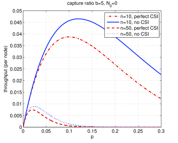
Figure 1: $n$ homogeneous nodes with perfect CSI and no CSI at the Nash equilibrium point under the SINR capture model with the capture ratio $b=5$ and $N_{0}/P_{T}\rightarrow 0$.

This Braess-like paradox is illustrated in Fig. 1 where $b=5$ and $N_{0}/P_{T}\rightarrow 0$. As the figure shows, with the same average transmission probability, the throughput of homogeneous nodes with perfect CSI is never larger than that of homogeneous nodes with no CSI. This means that in order to achieve the same average throughput demand $\rho$, homogeneous nodes with perfect CSI need to have the average transmission probability $p$ (the smaller solution) at the Nash equilibrium point not smaller than that (the smaller solution) with no CSI when $b>1$.

Discussion:

1. This Braess-like paradox is clearly due to the fact that, while improving a node’s received power by transmitting when the channel is better, the threshold strategy also increases the average interference seen by each node. As a result, the SINRs of the nodes are not necessarily higher. Thus, if a node could refrain from taking the best response strategy and be less selfish (e.g., by ignoring the CSI and transmitting with the same probability at all time slots), the other nodes would benefit. If all the nodes could do the same, every node would benefit and the performance would improve. However, for a particular node, doing so would be against its best interest given that it does not know the channels of the other nodes. In addition, an individual node would never be sure if the other nodes would also be altruistic, unless a centralized regularization is applied. Thus, centralized control and/or altruism (or cooperation) are necessary to improve the performance. How the optimal performance can be achieved by centralized control or cooperation is an interesting topic that needs further investigation, but is beyond the scope of this paper.

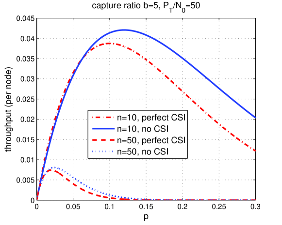
Figure 2: $n$ homogeneous nodes with perfect CSI and no CSI at the Nash equilibrium point under the SINR capture model with the capture ratio $b=5$ and $P_{T}/N_{0}=50$.

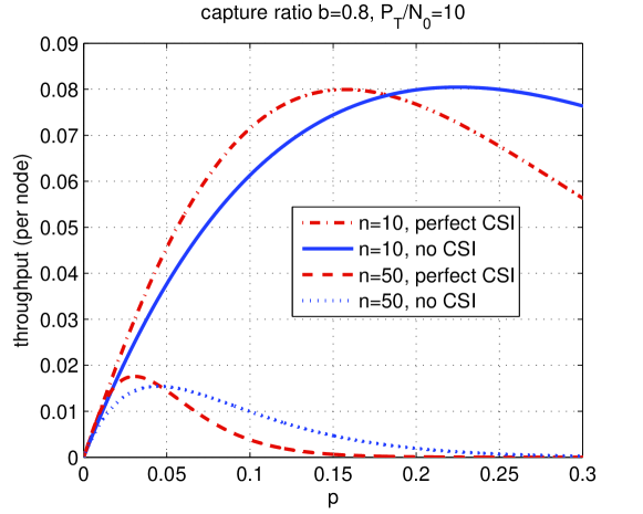
Figure 3: $n$ homogeneous nodes with perfect CSI and no CSI at the Nash equilibrium point under the SINR capture model with the capture ratio $b=0.8$ and $P_{T}/N_{0}=10$.

2. In general (when $N_{0}/P_{T}$ is not sufficiently small), Theorem 2 cannot be applied. The throughput comparison given the same average transmission probability depends on the average transmission probability $p$, the total number of nodes $n$, and the capture ratio $b$. Fig. 2 shows the cases with $b=5$ and $P_{T}/N_{0}=50$. It can be seen that when $n=10$ nodes, the throughput with perfect CSI is slightly higher than the throughput without CSI when the average transmission probability is smaller than 0.05. Fig. 3 is an example with $b=0.8$ and $P_{T}/N_{0}=10$. It is shown that there is no Braess-like paradox.

3. When $N_{0}=0$ and $b=\infty$, we have the collision model. In this case, the throughputs of homogeneous nodes with perfect CSI and without CSI will both be $p(1-p)^{n-1}$ when the average transmission probability is $p$.

4. For the case with heterogeneous nodes, the conditions for the occurrence of Braess-like paradoxes are quite complicated and need to be analyzed case by case. Here, we present a numerical example of a two-node network. Assume $b=5$ and $\frac{N_{0}}{P_{T}}=0.01$.

   • Case (i) $p_{1}=0.52$ and $p_{2}=0.24$: the throughput demands achievable for node 1 and node 2 without CSI availability are $\rho_{1}=0.3957$, $\rho_{2}=0.129$, respectively. With perfect CSI, the throughput demands achievable for node 1 and node 2 are $\rho_{1}=0.3952$, $\rho_{2}=0.118$, respectively. A Braess-like paradox occurs.

   • Case (ii) $p_{1}=0.580$ and $p_{2}=0.088$: the throughput demands achievable for node 1 and node 2 without CSI availability are $\rho_{1}=0.511$, $\rho_{2}=0.04325$, respectively. With perfect CSI, the throughput demands achievable for node 1 and node 2 are $\rho_{1}=0.529$, $\rho_{2}=0.04300$, respectively. The results show that it is possible that node 2 gains while node 1 suffers when CSI is available.

IV Power Capture Model

IV-A Equilibrium point analysis for power capture

We first analyze the case when CSI is not available. Let the PDF and the cumulative density function (CDF) of $|h_{i,k}|^{2}$ be $f(x)$ and $F(x)$, respectively. The received power $P_{i}$ of node $i$ at time $k$ is given by $B_{i,k}P_{T}|h_{i,k}|^{2}$ where $B_{i,k}=1$ if node $i$ transmits at time $k$ and $B_{i,k}=0$ otherwise. Then the average throughput of node $i$ is given by

$$r_{i}(p_{i},\textbf{p}_{-i}) =Pr\left[B_{i,k}|h_{i,k}|^{2}>\max_{j\neq i}\left\{(1+\Delta)B_{j,k}|h_{j,k}|^{2}\right\}\right]$$

$$=p_{i}\int_{0}^{\infty}\prod_{j\neq{}i}\left[\int_{0}^{\frac{{x_{i}}}{1+\Delta}}\!\!f(x_{j})dx_{j}\!+\!(1\!-\!p_{j})\int_{{\frac{{x_{i}}}{1+\Delta}}}^{\infty}\!\!f(x_{j})dx_{j}\right]\!f({x_{i}})d{x_{i}}$$

$$=p_{i}\int_{0}^{\infty}\prod_{j\neq{}i}\left[1-p_{j}\left(1-F\left({\frac{{x_{i}}}{1+\Delta}}\right)\right)\right]\!f({{x_{i}}})d{x_{i}}$$

$$=p_{i}\left\{1-\left(\sum_{j\neq{}i}p_{j}\right)\int_{0}^{\infty}\left(1-F\left(\frac{{x_{i}}}{1+\Delta}\right)\right)f({x_{i}})d{x_{i}}\right.$$

$$+\left(\sum_{(j,k)\in{}I_{-i}}p_{j}p_{k}\right)\int_{0}^{\infty}\left(1-F\left(\frac{{x_{i}}}{1+\Delta}\right)\right)^{2}f({x_{i}})d{x_{i}}$$

$$-\cdots$$

$$\left.+(-1)^{n-1}\left(\prod_{j\neq{}i}p_{j}\right)\int_{0}^{\infty}\left(1-F\left(\frac{{x_{i}}}{1+\Delta}\right)\right)^{n-1}f({x_{i}})d{x_{i}}\right\}$$

where the last equality is obtained by expanding the product terms in the integral, and the notation $(y_{1},y_{2},\ldots,y_{k})\in{}I_{-i}$ means that $y_{1}<y_{2}<\cdots<y_{k}$, all belonging to the node index set $I_{-i}\triangleq\{1,2,\ldots,n\}\setminus\{i\}$.

For Rayleigh fading channels, $f(x)$ is the exponential function, so we have

$$\int_{0}^{\infty}\left(1-F\left(\frac{{x_{i}}}{1+\Delta}\right)\right)^{n}f({x_{i}})d{x_{i}}=\frac{1+\Delta}{1+\Delta+n}.$$

Therefore, if $(p_{1},\ldots,p_{n})$ is a Nash equilibrium point, we have the following set of equations for the corresponding achievable average throughput demands

$$r_{i}(p_{i},\textbf{p}_{-i})=\rho_{i}=p_{i} -\frac{1+\Delta}{2+\Delta}\sum_{j\in{}I_{-i}}p_{i}p_{j}+\frac{1+\Delta}{3+\Delta}\!\sum_{(j,k)\in{}I_{-i}}\!\!p_{i}p_{j}p_{k}$$

$$-\cdots+(-1)^{n-1}\frac{1+\Delta}{n+\Delta}\prod^{n}_{j=1}p_{j},~{}~{}\forall{}i=1,\ldots,n,$$ (15)

and the resultant total achievable average throughput demand

$$\sum^{n}_{i=1}\rho_{i} \!=\!\sum^{n}_{i=1}p_{i}\!-\!\frac{2+2\Delta}{2+\Delta}\sum_{(i,j)\in{}I}p_{i}p_{j}\!+\!\frac{3+3\Delta}{3+\Delta}\sum_{(i,j,k)\in{}I}p_{i}p_{j}p_{k}$$

$$\hskip 32.52127pt-\cdots+(-1)^{n-1}\frac{n+n\Delta}{n+\Delta}\prod^{n}_{i=1}p_{i},$$ (16)

where the notation $(y_{1},y_{2},\ldots,y_{k})\in{}I$ means that $y_{1}<y_{2}<\cdots<y_{k}$, all belonging to the node index set $I\triangleq\{1,2,\ldots,n\}$.

Example 1 ($\Delta=\infty$)

The set of equations for a Nash equilibrium point become $\rho_{i}=p_{i}\prod_{j\neq i}(1-p_{j})$, i.e., the case $\Delta=\infty$ corresponds to the collision model, and there exist exactly two Nash equilibrium points for any throughput demands within the feasible region [12].

Example 2 ($\Delta=0$)

For the special case where $\Delta=0$, i.e., perfect power capture model, we have

$$\rho_{i}=p_{i} -\frac{1}{2}\sum_{j\in{}I_{-i}}p_{i}p_{j}+\frac{1}{3}\!\sum_{(j,k)\in{}I_{-i}}\!\!p_{i}p_{j}p_{k}$$

$$-\cdots+\frac{(-1)^{n-1}}{n}\prod^{n}_{j=1}p_{j},$$ (17)

and the total achievable average throughput demand

$$\sum^{n}_{i=1}\rho_{i} =\sum^{n}_{i=1}p_{i}-\sum_{(i,j)\in{}I}p_{i}p_{j}+\sum_{(i,j,k)\in{}I}p_{i}p_{j}p_{k}$$

$$\ \ \ -\cdots+(-1)^{n-1}\prod^{n}_{i=1}p_{i}$$

$$=1-\prod^{n}_{i=1}(1-p_{i}).$$ (18)

The following theorem shows that there exists a unique Nash equilibrium point:

Theorem 3

Under the perfect power capture model ($\Delta=0$) with no CSI available to all nodes, there exists a unique Nash equilibrium point for the average throughput demands $(\rho_{1},\ldots,\rho_{n}),\rho_{i}\geq{}0,\forall{}i$, if and only if

$$\sum^{n}_{i=1}\rho_{i}\leq{}1$$

Proof:

In Appendix -A.

∎

In the case when perfect CSI is available to all nodes, a particular node $i$ will transmit only when its CSI is larger than a threshold $T_{i}$. $T_{i}$ must satisfy $\int^{\infty}_{T_{i}}f(x_{i})dx_{i}=e^{-T_{i}}=p_{i}$, where $p_{i}$ is the average transmission probability of node $i$, and $f(\cdot)$ is the exponential PDF for Rayleigh fading channels. The average throughput of node $i$ can be computed as

$$r_{i}(p_{i},\textbf{p}_{-i}) =\int_{T_{i}}^{\infty}\prod_{j\neq{}i}\left[\int_{0}^{T_{j}}\!\!f(x_{j})dx_{j}\!+\!\int_{T_{j}}^{\max\left\{\frac{x_{i}}{1+\Delta},~{}T_{j}\right\}}\!\!f(x_{j})dx_{j}\right]\!f(x_{i})dx_{i}$$

$$=\int_{T_{i}}^{\infty}\prod_{j\neq{}i}\left[\max\left\{1-p_{j},~{}1-e^{-\frac{x_{i}}{1+\Delta}}\right\}\right]\!f(x_{i})dx_{i}.$$ (19)

This expression depends on the specific values of the thresholds (hence the average transmission probabilities and the average throughput demands) of individual nodes.

In the following, we will only consider the case with homogeneous nodes. Let the throughput demands be $(\rho,\ldots,\rho)$ and the Nash equilibrium point $(p_{1},\ldots,p_{n})=(p,\ldots,p)$. When CSI is not available to all nodes, from (IV-A) we have

$$r_{i}(p,\ldots,p)=\rho=p\!-\!{{n-1}\choose{1}}\frac{1+\Delta}{2+\Delta}p^{2}\!+\!\cdots\!+\!(-1)^{n-1}{{n-1}\choose{n-1}}\frac{1+\Delta}{n+\Delta}p^{n}.$$ (20)

In the case when perfect CSI is available to all nodes, a node will transmit only when its CSI is larger than a threshold $T$. $T$ must satisfy $\int^{\infty}_{T}f(x)dx=e^{-T}=p$, where $p$ is the average transmission probability. For this case, denote the average throughput demand achievable at the Nash equilibrium point $(p,\ldots,p)$ as $\rho^{\prime}$. We have

$$r_{i}(p,\ldots,p)=\rho^{\prime}= \int^{(1+\Delta)T}_{T}\left[\prod_{j\neq i}\int^{T}_{0}f(x_{j})dx_{j}\right]f({x_{i}})d{x_{i}}$$

$$+\int^{\infty}_{(1+\Delta)T}\left[\prod_{j\neq i}\int^{\frac{{x_{i}}}{1+\Delta}}_{0}f(x_{j})dx_{j}\right]f({x_{i}})d{x_{i}}$$

$$= \left[p(1-p)^{n-1}(1-p^{\Delta})\right]\!+\!\Big{[}p^{1+\Delta}-{{n-1}\choose{1}}\frac{1+\Delta}{2+\Delta}p^{2+\Delta}$$

$$+\cdots+(-1)^{n-1}{{n-1}\choose{n-1}}\frac{1+\Delta}{n+\Delta}p^{n+\Delta}\Big{]}.$$ (21)

The Nash equilibrium can be analyzed as follows when perfect CSI is available to homogeneous nodes. From (IV-A), we have $\frac{dr_{i}}{dp}=(1-p)^{n-2}\left[1-np+(n-1)p^{1+\Delta}\right]$, and

$$\frac{d}{dp}\left(1-np+(n-1)p^{1+\Delta}\right)=-n+(n-1)(1+\Delta)p^{\Delta}.$$ (22)

Note that $1-np+(n-1)p^{1+\Delta}=1$ if $p=0$, and $1-np+(n-1)p^{1+\Delta}=0$ if $p=1$. We consider two cases: $0\leq\Delta\leq\frac{1}{n-1}$ and $\Delta>\frac{1}{n-1}$ separately in the following.

• Case (i) $0\leq\Delta\leq\frac{1}{n-1}$: From (22), $1-np+(n-1)p^{1+\Delta}$ is a decreasing function for $p\in[0,1]$, so $\frac{dr_{i}}{dp}\geq 0$ when $0\leq\Delta\leq\frac{1}{n-1}$. This means that $r_{i}$ is an increasing function in $p$, so there exists a unique Nash equilibrium point if the throughput demand is achievable under the case $0\leq\Delta\leq\frac{1}{n-1}$.

• Case (ii) $\Delta>\frac{1}{n-1}$: $1-np+(n-1)p^{1+\Delta}$ has a minimum at $p^{*}=\left[\frac{n}{(n-1)(1+\Delta)}\right]^{\frac{1}{\Delta}}\in(0,1)$, and $1-np+(n-1)p^{1+\Delta}$ is decreasing in $(0,p^{*})$ and increasing in $(p^{*},1)$. Therefore, $1-np+(n-1)p^{1+\Delta}$ has exactly two zeros $z_{1}$, $z_{2}(=1)$ in $[0,1]$. It follows that $\frac{dr_{i}}{dp}\geq 0$ in $[0,z_{1}]$ and $\frac{dr_{i}}{dp}\leq 0$ on $[z_{1},1]$. In other words, $r_{i}$ increases to the maximum $\rho^{\prime}_{max}$ when the transmission probability $p$ is from $p=0$ to $p=z_{1}$ and then decreases when $p>z_{1}$. This means that there exist at most two Nash equilibrium points if the throughput demand is achievable (i.e., $\rho^{\prime}\leq\rho^{\prime}_{max}$) under the case $\Delta>\frac{1}{n-1}$.

IV-B Braess-like paradox for power capture

We present analytically a Braess-like paradox for the case with homogeneous nodes by the following theorem.

Theorem 4

With the same average transmission probability $p$ (or average power investment), the achievable average throughput demand of homogeneous nodes with perfect CSI is not larger than that of homogeneous nodes without CSI under the power capture model.

Proof:

We want to show $\rho^{\prime}\leq\rho$, where $\rho^{\prime}$ and $\rho$ are given in (20) and (IV-A), respectively. We have

$$\rho^{\prime}= (1-p^{\Delta})p(1-p)^{n-1}+p^{\Delta}\rho$$

$$\leq \max\{p(1-p)^{n-1},\rho\}$$

$$\leq \rho,$$

where the first inequality is deduced from the convex combination of $p(1-p)^{n-1}$ and $\rho$, and the second inequality is due to the fact that $p(1-p)^{n-1}$ equals to the throughput for $\Delta=\infty$ (when CSI is not available) and the throughput decreases as $\Delta$ increases. The proof is complete. ∎

Similarly, this theorem implies a Braess-like paradox that for the same achievable average throughput demand $\rho$, homogeneous nodes with perfect CSI have the average transmission probability $p$ (or average power investment) at the Nash equilibrium point not smaller than that of the case without CSI.

V Distributed Algorithms

In a network, each node can usually estimate its average throughput through, for example, the acknowledgement of successful packet reception from the BS. Let $\hat{\rho}_{i}$ denote node $i$’s throughput estimate. We can set node $i$’s initial (i.e., at the $0$th iteration) transmission probability $p_{i}(0)=\rho_{i}$, as the transmission probability needs to be at least $\rho_{i}$ to fulfill the throughput demand. We provide one most common distributed mechanism converging to the Nash equilibrium point. The readers are referred to [8][14][12] for more discussions on the use of various distributed algorithms to achieve the equilibrium points in random access games.

At the ($m+1$)th iteration, each node updates its transmission probability by

$$p_{i}(m+1)=p_{i}(m)+\epsilon(m)\left[\min\left(1,\frac{\rho_{i}}{\hat{\rho}_{i}(m)}p_{i}(m)\right)-p_{i}(m)\right],$$

where the step size $\epsilon(m)>0$. Usually, $\epsilon(m)\leq 1$, for example, $\epsilon(m)=\frac{1}{1+m}$ and a smaller $\epsilon(m)$ will more likely ensure the convergence to the better Nash equilibrium point (i.e., $\sum p_{i}\leq\frac{b+1}{b}$) under the SINR capture model, and to the unique Nash equilibrium under the power capture model. However, it also takes a longer time for convergence. When CSI is available, the threshold $T_{i}(m+1)$ can be uniquely determined from $p_{i}(m+1)$ and vice versa if the channel characteristics are known. Note that the time between two consecutive iterations of a node does not have to be the same as that of the other nodes. The nodes can update their transmission probabilities synchronously or asynchronously.

Issues such as infeasible throughput demands, and the design tradeoff of $\epsilon(m)$ between ensuring convergence and the convergence time, are beyond the scope of this paper.

We present some simulation results in Fig. 4 and Fig. 5, where the channels are i.i.d. Rayleigh fading, and the reception model is SINR capture. We consider a three-node network with throughput demands $\rho_{1}=0.10$, $\rho_{2}=0.05$, $\rho_{3}=0.01$, the capture ratio $b=5$, and $\frac{P_{T}}{N_{0}}=10$. The cases with no CSI and perfect CSI are considered, and node $i$ estimates its $\hat{\rho}_{i}$ by the number of successfully transmitted packets divided by number of time slots that have elapsed. For the case with no CSI, the dynamic of the transmission probabilities is plotted in Fig. 4. For the case with perfect CSI, we have the threshold $T_{i}(m+1)=-\ln p_{i}(m+1)$, and node $i$ will transmit only if its channel gain is larger than the threshold $T_{i}$. The dynamic of the thresholds is plotted in Fig. 5. Three realizations are shown for each case, and the figures illustrate that they indeed converge to the same equilibrium.

VI Conclusion

In this paper, we used a game-theoretic approach to study the Nash equilibrium point of CSI-dependent transmission probabilities for selfish random access nodes in fading channels with capture. The analysis revealed that under the power capture and SINR capture models, there are at most two Nash equilibrium points in the feasible region of throughput demands. For the collision channel, which is a special case of both the power capture and SINR capture models, there are exactly two Nash equilibrium points within the feasible region. On the other hand, there is one unique Nash equilibrium point under the perfect power capture model when CSI is not available to selfish nodes. Our work extends the existing works in the literature. Moreover, we pointed out that, in some situations, performance degradation may occur when CSI is available to selfish random access nodes as compared to when CSI is not available. We called this phenomenon a Braess-like paradox. In particular, we analytically showed that for homogeneous nodes, Braess-like paradoxes occur in the power capture model and in the SINR capture model with the capture ratio larger than one and noise to signal ratio sufficiently small.

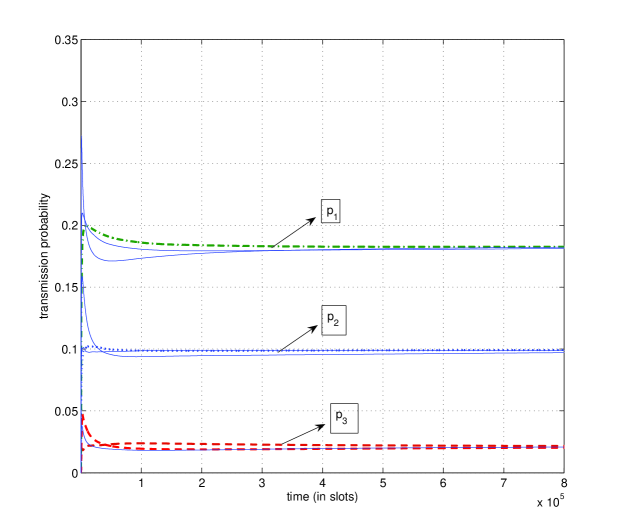
Figure 4: Dynamic of transmission probabilities in a three-node network with no CSI under the SINR capture model. The capture ratio $b=5$, $\frac{P_{T}}{N_{0}}=10$, and the throughput demands are $\rho_{1}=0.10$, $\rho_{2}=0.05$, $\rho_{3}=0.01$.

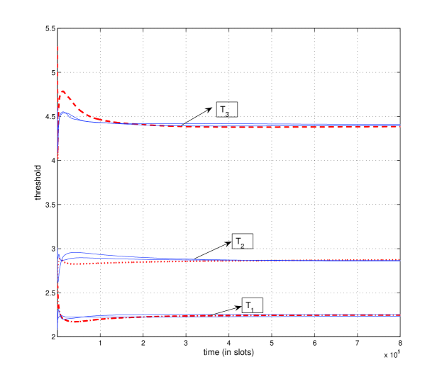
Figure 5: Dynamic of thresholds in a three-node network with perfect CSI under the SINR capture model. The capture ratio $b=5$, $\frac{P_{T}}{N_{0}}=10$, and the throughput demands are $\rho_{1}=0.10$, $\rho_{2}=0.05$, $\rho_{3}=0.01$.

References

- [1] N. Abramson, “The ALOHA system – another alternative for computer communications,” in Proc. AFIPS Conf., 1970.
- [2] L. G. Roberts, “ALOHA packet system with and without slots and capture,” Stanford Res. Inst., Advanced Research Projects Agency, Network Information Center, Stanford, Tech. Rep. ASS Note 8, 1972.
- [3] M. Zorzi, “Mobile radio slotted ALOHA with capture and diversity,” Wireless Networks, vol. 1, no. 2 pp. 227–239, 1995.
- [4] A. B. MacKenzie and S. B. Wicker, “Selfish users in Aloha: a game-theoretic approach,” in Proc. IEEE VTC, Fall 2001.
- [5] M. J. Osborne and A. Rubinstein, A Course in Game Theory, The MIT Press, 1994.
- [6] H. Inaltekin and S. B. Wicker, “The analysis of nash equilibria of the one-shot random-access game for wireless networks and the behavior of selfish nodes,” IEEE/ACM Trans. Netw., vol. 16, no. 5, pp. 1094–1107, Oct. 2008.
- [7] A. B. MacKenzie and S. B. Wicker, “Game theory and the design of self-configuring, adaptive wireless networks,” IEEE Commun. Mag., pp. 126–131, Nov. 2001.
- [8] T. Cui, L. Chen, and S. H. Low, “A game-theoretic framework for medium access control,” IEEE J. Sel. Areas Commun., vol. 26, no. 7, pp. 1116–1127, Sept. 2008.
- [9] J.-W. Lee, A. Tang, J. Huang, M. Chiang, and A. R. Calderbank, “Reverse-engineering MAC: a non-cooperative game model,” IEEE J. Sel. Areas Commun., vol. 25, no. 6, pp. 1135–1147, Aug. 2007.
- [10] D. Braess, A. Nagurney, and T. Wakolbinger, “On a paradox of traffic planning” Transp. Sci., vol. 39, no. 4, pp. 446–450, Nov. 2005.
- [11] Y. Jin and G. Kesidis “Equilibria of a noncooperative game for heterogeneous users of an Aloha network,” IEEE Comm. Letters, vol. 6, no. 7, pp. 282–284, 2002.
- [12] I. Menache and N. Shimkin, “Rate-based equilibria in collision channels with fading,” IEEE J. Sel. Areas Commun., vol. 26, no. 7, pp. 1070–1077, Sept. 2008.
- [13] I. Menache and N. Shimkin, “Decentralized rate regulation in random access channels,” in Proc. IEEE INFOCOM, 2008.
- [14] E. Sabir, R. El-Azouzi, V. Kavitha, Y. Hayel, and E.-H. Bouyakhf, “Stochastic learning solution for constrained Nash equilibrium throughput in non saturated wireless collision channels,” in Proc. ICST/ACM GameComm (in conjunction with ValueTools), 2009.
- [15] M. H. Ngo and V. Krishnamurthy, “Game theoretic cross-layer transmission policies in multipacket reception wireless networks,” IEEE Trans. Signal Process., vol. 55, no. 5, pp. 1911–1926, May 2007.
- [16] S. Ghez, S. Verdú, and S. Schwartz, “Stability properties of slotted-Aloha with multi-packet reception capability,” IEEE Trans. Automat. Contr., vol. 33, no. 7, pp. 640–649, July 1988.
- [17] V. Naware, G. Mergen, and L. Tong, “Stability and delay of finite-user slotted ALOHA with multipacket reception,” IEEE Trans. Inf. Theory, vol. 51, no. 7, pp. 2636–2656, July 2005.
- [18] J. Sun and E. Modiano, “Opportunistic power allocation for fading channels with non-cooperative users and random access,” in Proc. BroadNets, 2005.
- [19] I. Menache and N. Shimkin, “Noncooperative power control and transmission scheduling in wireless collision channels,” in Proc. ACM SIGMETRICS, 2008.
- [20] P. Gupta and P. R. Kumar, “The Capacity of Wireless Networks,” IEEE Trans. Inf. Theory, vol. 46, no. 2, pp. 388–404, Mar. 2000.
- [21] J. E. Cohen and C. Jeffries, “Congestion resulting from increased capacity in single-server queueing networks,” IEEE/ACM Trans. Netw., vol. 5, no. 2, pp. 305–310, Apr. 1997.
- [22] Y. A. Korilis, A. A. Lazar, and A. Orda, “Avoiding the Braess paradox in non-cooperative networks,” J. Appl. Prob., vol. 36, pp. 211–222, 1999.
- [23] H. Kameda, E. Altman, T. Kozawa, and Y. Hosokawa, “Braess-like paradoxes in distributed computer systems,” IEEE Trans. Automat. Contr., vol. 45, no. 9, pp. 1687–1691, Sept. 2000.
- [24] H. Kameda and O. Pourtallier, “Paradoxes in distributed decisions on optimal load balancing for networks of homogeneous computers,” J. ACM, vol. 49, No. 3, pp. 407–433, May 2002.
- [25] A. Tang, J. Wang, and S. H. Low, “Counter-intuitive throughput behaviors in networks under end-to-end control,” IEEE/ACM Trans. Netw., vol. 14, no. 2, pp. 355–368, Apr. 2006.
- [26] E. Altman, V. Kamble, and H. Kameda, “A Braess type paradox in power control over interference channels,” in Proc. WiOpt, 2008.
- [27] A. B. MacKenzie and S. B. Wicker, “Stability of multipacket slotted Aloha with selfish users and perfect information,” in Proc. IEEE INFOCOM, 2003.
- [28] J. G. Proakis, Digital Communications, McGraw-Hill Company, 4th ed., 2001.
- [29] D. J. Goodman and N. B. Mandayam, “Power control for wireless data,” IEEE Personal Commun. Mag., vol. 7, no. 2, pp. 48–54, Apr. 2000.
- [30] A. Dua, “Random access with multi-packet reception,” IEEE Trans. Wireless Comm., vol. 7, no. 6, pp. 2280–2288, June 2008.