Quantum and thermal Casimir interaction between a sphere and a plate:
Comparison of Drude and plasma models

Abstract

We calculate the Casimir interaction between a sphere and a plate, both described by the plasma model, the Drude model, or generalizations of the two models. We compare the results at both zero and finite temperatures. At asymptotically large separations we obtain analytical results for the interaction that reveal a non-universal, i.e., material dependent interaction for the plasma model. The latter result contains the asymptotic interaction for Drude metals and perfect reflectors as different but universal limiting cases. This observation is related to the screening of a static magnetic field by a London superconductor. For small separations we find corrections to the proximity force approximation (PFA) that support correlations between geometry and material properties that are not captured by the Lifshitz theory. Our results at finite temperatures reveal for Drude metals a non-monotonic temperature dependence of the Casimir free energy and a negative entropy over a sizeable range of separations.

I Introduction

The past decade has witnessed rapid progress in the precision of Casimir force measurements Lamoreaux (1997); Mohideen and Roy (1998); Harris et al. (2000); Decca et al. (2005, 2007); Klimchitskaya et al. (2009). The measurement precision that is expected in the near future demands accurate theoretical calculations of the Casimir force for the geometries and materials used in experiments. While Casimir’s original calculation for perfect metal plates Casimir (1948) and Lifshitz’s formula for dielectric slabs Dzyaloshinskii et al. (1961) only apply to planar, parallel surfaces, recent measurements have set limits on geometry induced corrections in the most frequently used sphere-plate geometry Krause et al. (2007). The geometry dependence of Casimir forces is intriguing as it can vary substantially with the shape and relative orientation of the objects Emig et al. (2009); Rahi et al. (2009); Bordag et al. (2009). Material dependence in the form of dissipation in metals has been experimentally confirmed to have an effect on the Casimir force Decca et al. (2007); Chen et al. (2007). It is thus important that the geometry and material dependence be carefully investigated for the experimentally most important sphere-plate configuration.

In order to compare the experimental results to theory, the Derjaguin or proximity force approximation (PFA) Parsegian (2005) has commonly been used. This approximation neglects the non-additivity of Casimir forces by estimating the interaction between curved surfaces in terms of the planar surface interaction between infinitesimal and parallel surface elements. Its validity is hence limited to the singular limit of vanishingly small separations between the surfaces. A systematic extension to larger separations is not possible within such approximations.

The first exact computation of the Casimir interaction energy for a perfectly reflecting sphere and plate was presented in Ref. Emig (2008). Recently, corrections that come from using the plasma or Drude model were computed at zero temperature Canaguier-Durand et al. (2009) and at $T=300^{\circ}K$ Canaguier-Durand et al. (2010). Other open geometries with curvature such as a cylinder above a plate have been studied for perfect metals Emig et al. (2006). Corrections to the PFA in the case of perfect metals for a cylinder above a plate and a sphere above a plate have been obtained using path integral approaches Bordag (2006); Bordag and Nikolaev (2009) and for scalar fields employing a world line formalism Gies and Klingmuller (2006).

Here we show that Casimir forces reveal a rich interplay between geometry (radius of the sphere and object’s separation), optical properties of metals and thermal fluctuations. We study this in detail by calculating the Casimir interaction for different sphere radii and separations using the (i) the Drude model, (ii) a generalized Drude model, (iii) the plasma model and (iv) a generalized plasma model at different temperatures. The study of these combined effects is of utmost importance since Casimir force measurements continue to be carried out using this geometry and an increasing accuracy is expected. Hence, the experimental findings will begin to show sensitivity to the material and temperature effects, which we take into account here. Furthermore, the unabated controversy whether the plasma or the Drude model is more appropriate for describing the optical properties of metals in Casimir calculations compels us to provide results for both models so that experimentalists can build on them when studying this problem further. The plasma model is a high-frequency description of the optical properties and the divergence $\sim 1/\omega^{2}$ of its dielectric function for small $\omega$ is unphysical for metals. The Drude model provides a proper low-frequency description for metals with a $1/\omega$ divergence of the dielectric function for small $\omega$. At large frequencies, both models become identical.

Below, we supply numerical results for the Casimir interaction at arbitrary separations as well as analytic formulas for the asymptotic interaction at large separations. Depending on the model under consideration, the asymptotic results show universal or non-universal (i.e., material-independent or -dependent) behavior, a feature which is not present for the simple case of two parallel metal plates and hence results from the interplay of finite object sizes and material properties.

II General expression for the interaction

To calculate the interaction of a metallic sphere of radius $R$ and a metallic plate with a separation $d$ between the center of the sphere and the plate, we employ a scattering approach for Casimir interactions, which is described in detail in Ref. Rahi et al. (2009). The Casimir free energy of this system at temperature $T$ is given by

$$E=k_{B}T{\sum_{n=0}^{\infty}}^{\prime}\log\det[1-Y(\kappa_{n})]\,,$$ (1)

with Matsubara wave numbers $\kappa_{n}=2\pi nk_{B}T/\hbar c$. The primed sum indicates that the contribution for $n=0$ is to be weighted by a factor of $1/2$. At zero temperature the sum is replaced by an integral along the imaginary frequency axis Rahi et al. (2009),

$$E=\frac{\hbar c}{2\pi}\int_{0}^{\infty}d\kappa\log\det[1-Y(\kappa)]\,,$$ (2)

where the matrix $Y$ is given by the product

$$Y^{\alpha\beta}_{lml^{\prime}m^{\prime}}=T_{s,lm}^{\alpha}U_{lml^{\prime}m}^{\alpha\beta}\delta_{mm^{\prime}}$$ (3)

of the T-operator $T_{s}$ of the sphere and an operator $U$ that describes the propagation of waves between the plate and the sphere and the scattering of them at the plate (see below). We represent these operators in a vector basis of spherical waves, where $\alpha$, $\beta$=E, M denote electric or magnetic multipoles and $l$, $m$ label the spherical waves. For a sphere of radius $R$ with uniform permittivity $\epsilon(\omega)$ and permeability $\mu(\omega)$ the T-matrix elements for M-multipoles are given by

$$T^{\textsc{m}}_{s,lm}=\frac{\pi}{2}\frac{\eta I_{l+{1\over 2}}(\kappa R)\left[I_{l+{1\over 2}}(n\kappa R)+2n\kappa RI^{\prime}_{l+{1\over 2}}(n\kappa R)\right]-nI_{l+{1\over 2}}(n\kappa R)\left[I_{l+{1\over 2}}(\kappa R)+2\kappa RI^{\prime}_{l+{1\over 2}}(\kappa R)\right]}{\eta K_{l+{1\over 2}}(\kappa R)\left[I_{l+{1\over 2}}(n\kappa R)+2n\kappa RI^{\prime}_{l+{1\over 2}}(n\kappa R)\right]-nI_{l+{1\over 2}}(n\kappa R)\left[K_{l+{1\over 2}}(\kappa R)+2\kappa RK^{\prime}_{l+{1\over 2}}(\kappa R)\right]}\,,$$ (4)

with $n=\sqrt{\epsilon(i\kappa)\mu(i\kappa)}$, $\eta=\sqrt{\epsilon(i\kappa)/\mu(i\kappa)}$. The T-matrix elements for E-multipoles, $T^{\textsc{e}}_{s,lm}$, are obtained from Eq. (4) by interchanging $\epsilon$ and $\mu$ and by changing the overall sign. By taking $\epsilon(i\kappa)\to\infty$ at an arbitrarily fixed $\mu(i\kappa)$ in Eq. (4), the limit of a perfectly reflecting sphere and plate is obtained. Then the matrix elements become independent of $\mu$,

$$T^{\textsc{m}}_{s,lm} =\frac{\pi}{2}\frac{I_{l+{1\over 2}}(\kappa R)}{K_{l+{1\over 2}}(\kappa R)}$$ (5a)

$$T^{\textsc{e}}_{s,lm} =-\frac{\pi}{2}\frac{I_{l+{1\over 2}}(\kappa R)+2\kappa RI^{\prime}_{l+{1\over 2}}(\kappa R)}{K_{l+{1\over 2}}(\kappa R)+2\kappa RK^{\prime}_{l+{1\over 2}}(\kappa R)}\,.$$ (5b)

These matrix elements scale for small $\kappa$ as $\kappa^{2l+1}$. It is interesting to compare this behavior to the scaling of the general matrix elements of Eq. (4) for the dielectric functions of the Drude and plasma model. For both models the $T^{\textsc{e}}_{s,lm}\sim\kappa^{2l+1}$ behavior is unchanged for E-multipoles. The coefficients become material (plasma frequency) dependent for the plasma model but retain the universal values of a prefect reflector for the Drude model. However, for M-multipoles only the plasma model shows this universal behavior while the Drude model yields a different scaling $T^{\textsc{m}}_{s,lm}\sim\kappa^{2l+2}$ with non-universal conductivity dependent coefficients.

The operator $U$ can also be expressed in a spherical wave basis. It describes the propagation of waves from the sphere to the plate, a reflection at the plate and the propagation back to the sphere. The reflection of waves at a dielectric plane is described most easily in a plane wave basis with in-plane wave vector $k_{\|}$. The T-matrix elements of the plane are then given by the usual Fresnel coefficients. The conversion from plane to spherical waves and simultaneous translation from the sphere to the plane is obtained by multiplying the plane’s T-matrix from left and right by a matrix $D^{\alpha\beta}_{lm}(k_{\|})$. After defining $z=k_{\|}/\kappa$, the matrix multiplication runs over the continuous variable $z$ and the elements of the operator $U$ can be written as

$$U_{lml^{\prime}m}^{\alpha\beta}\!=\!\!\!\int_{0}^{\infty}\!\!\frac{zdz}{4\pi}\frac{e^{-2d\kappa\sqrt{1+z^{2}}}}{\sqrt{1+z^{2}}}\!\!\sum_{\gamma}\!D^{\alpha\gamma}_{lm}(z)T_{p}^{\gamma}(\kappa,z){D_{l^{\prime}m}^{\beta\gamma}}^{*}(z)\,,$$ (6)

where the plate’s diagonal T-matrix, $T_{p}^{\gamma}(\kappa,z)$, for polarization $\gamma$ are given by

$$T_{p}^{\textsc{M}} =-\frac{\mu(i\kappa)\sqrt{1+z^{2}}-\sqrt{\epsilon(i\kappa)\mu(i\kappa)+z^{2}}}{\mu(i\kappa)\sqrt{1+z^{2}}+\sqrt{\epsilon(i\kappa)\mu(i\kappa)+z^{2}}}\,,$$ (7a)

$$T_{p}^{\textsc{E}} =\frac{\epsilon(i\kappa)\sqrt{1+z^{2}}-\sqrt{\epsilon(i\kappa)\mu(i\kappa)+z^{2}}}{\epsilon(i\kappa)\sqrt{1+z^{2}}+\sqrt{\epsilon(i\kappa)\mu(i\kappa)+z^{2}}}\,.$$ (7b)

The exponential factor in Eq. (6) describes the translation from the sphere to the plane and back by a total distance $2d$ in the plane wave basis. The elements of the matrix that converts between plane and spherical waves are given by

$$D^{\textsc{MM}}_{lm} =D^{\textsc{EE}}_{lm}=\sqrt{\frac{4\pi(2l+1)(l-m)!}{l(l+1)(l+m)!}}z{P_{l}^{m}}^{\prime}\left(\sqrt{1+z^{2}}\right)\,,$$ (8a)

$$D^{\textsc{EM}}_{lm} =-D^{\textsc{ME}}_{lm}=\sqrt{\frac{4\pi(2l+1)(l-m)!}{l(l+1)(l+m)!}}\frac{im}{z}P_{l}^{m}\left(\sqrt{1+z^{2}}\right),$$ (8b)

where $P_{l}^{m}$ is the associated Legendre polynomial of order $l$, $m$. These elements have the following symmetries under complex conjugation,

$${D^{\alpha\alpha}_{lm}}^{*} =(-1)^{m}D^{\alpha\alpha}_{lm}\,$$ (9a)

$${D^{\textsc{ME}}_{lm}}^{*} =(-1)^{m+1}D^{\textsc{ME}}_{lm}\,.$$ (9b)

In what follows we employ Eqs. (1), (2) to obtain the Casimir interaction for perfectly reflecting bodies and also for metals described by the plasma and Drude model at zero and finite temperatures.

III Large distance interaction at $T=0$

In this section we consider the zero temperature Casimir interaction at large separations for different dielectric functions.

III.1 Perfect reflector

In the limit of perfect reflectivity of the plate, one finds from Eq. (7) with $\epsilon\to\infty$ the simple T-matrix elements $T_{p}^{\textsc{M}}=T_{p}^{\textsc{E}}=1$. With this simplification, the integration over $z$ in Eq. (6) can be performed analytically. We find for the elements of $U$ the same result that was obtained before, using the method of images Emig (2008),

$$U^{\textsc{MM}}_{lml^{\prime}m} = U^{\textsc{EE}}_{lml^{\prime}m}=(-1)^{l+l^{\prime}+1}\sum_{l^{\prime\prime}=|l-l^{\prime}|}^{l+l^{\prime}}\frac{(-1)^{l^{\prime\prime}}}{2}\left[l(l+1)+l^{\prime}(l^{\prime}+1)-l^{\prime\prime}(l^{\prime\prime}+1)\right]\sqrt{\frac{(2l+1)(2l^{\prime}+1)}{l(l+1)l^{\prime}(l^{\prime}+1)}}(2l^{\prime\prime}+1)$$ (10)

$$\times\begin{pmatrix}l^{\prime}&l&l^{\prime\prime}\\ 0&0&0\end{pmatrix}\begin{pmatrix}l^{\prime}&l&l^{\prime\prime}\\ m&-m&0\end{pmatrix}\frac{K_{l^{\prime\prime}+1/2}(2\kappa d)}{\sqrt{\pi\kappa d}}$$

$$U^{\textsc{ME}}_{lml^{\prime}m} = -U^{\textsc{EM}}_{lml^{\prime}m}=(-1)^{l+l^{\prime}+1}2i\kappa dm\sum_{l^{\prime\prime}=|l-l^{\prime}|}^{l+l^{\prime}}(-1)^{l^{\prime\prime}}\sqrt{\frac{(2l+1)(2l^{\prime}+1)}{l(l+1)l^{\prime}(l^{\prime}+1)}}(2l^{\prime\prime}+1)$$ (11)

$$\times\begin{pmatrix}l^{\prime}&l&l^{\prime\prime}\\ 0&0&0\end{pmatrix}\begin{pmatrix}l^{\prime}&l&l^{\prime\prime}\\ m&-m&0\end{pmatrix}\frac{K_{l^{\prime\prime}+1/2}(2\kappa d)}{\sqrt{\pi\kappa d}}\,.$$

Using this result and the T-matrix elements of Eq. (5) we obtain for the interaction energy the large distance expansion

$$E=-\frac{\hbar c}{\pi}\left(\frac{9}{16}\frac{R^{3}}{d^{4}}+\frac{25}{32}\frac{R^{5}}{d^{6}}+{\cal O}(R^{6}/d^{7})\right)$$ (12)

at zero temperature Emig (2008).

III.2 Plasma model

We now assume that both the sphere and the plate are described by the plasma model which on the imaginary frequency axis has the dielectric function

$$\epsilon_{p}(ic\kappa)=1+\left(\frac{2\pi}{\lambda_{p}\kappa}\right)^{2}$$ (13)

The plasma wavelength $\lambda_{p}$ is related to the plasma frequency $\omega_{p}$ by $\lambda_{p}=2\pi c/\omega_{p}$. Note that the plasma model provides a high-frequency description of optical properties and ignores dissipation. Hence it is not expected to capture the low frequency response of a metal. To understand the physical meaning of the results for the Casimir interaction presented below, it is interesting to realize that the dielectric function of Eq. (13) appears also in the wave equation for the magnetic field in a superconductor when it is described by the London theory. The second London equation and the Maxwell equations yield $\epsilon_{p}$ with the penetration depth $\lambda_{p}=\sqrt{m_{e}c^{2}/(16\pi^{3}n_{s}e^{2})}$ for superfluid carriers of density $n_{s}$, charge $e$ and mass $m_{e}$.

To obtain the large distance behavior of the Casimir energy, we need to expand the T-matrices for small $\kappa$. To this end, we set $\kappa=u/d$ and expand the relevant expressions in powers of $1/d$. The T-matrix elements of the sphere scale as $\kappa^{2l+1}$ for $\kappa\to 0$ for both E and M polarizations. In the case of the E polarization the coefficients are universal and are given by the perfect reflector result which corresponds to

$$T^{\textsc{E}}_{s,lm}=\frac{l+1}{l}\frac{1}{(2l+1)!!(2l-1)!!}(uR/d)^{2l+1}+\ldots\,.$$ (14)

However, for the M polarization the coefficients are not universal and depend on the plasma wave length as follows

$$T^{\textsc{M}}_{s,lm}=\frac{I_{l+{3\over 2}}(2\pi R/\lambda_{p})}{I_{l-{1\over 2}}(2\pi R/\lambda_{p})}\frac{1}{(2l+1)!!(2l-1)!!}(uR/d)^{2l+1}+\ldots\,.$$ (15)

In the limit of a small plasma wavelength, $\lambda_{p}\ll R$, the elements of this matrix approach the perfect reflector limit with is given by

$$T^{\textsc{M}}_{s,lm}=\frac{1}{(2l+1)!!(2l-1)!!}(uR/d)^{2l+1}+\ldots\,.$$ (16)

For a large plasma wavelength, $\lambda_{p}\gg R$, the elements are not universal and reduced by a factor $(R/\lambda_{p})^{2}$ compared to the perfect reflector limit,

$$T^{\textsc{M}}_{s,lm}=\frac{(2\pi R/\lambda_{p})^{2}}{(2l+1)!!(2l+3)!!}(uR/d)^{2l+1}+\ldots\,.$$ (17)

The latter result can be understood in terms of the London superconductor interpretation of the plasma model. If the penetration depth $\lambda_{p}$ becomes much larger than the radius, the sphere becomes almost transparent for the magnetic field and the T-matrix elements are reduced to small values $\sim R^{2l+3}/\lambda_{p}^{2}$.

The T-matrix elements of the plate with $\epsilon_{p}(ic\kappa)$ of Eq. (13) depend also on the lateral wave vector ${\bf k}_{\|}$. To obtain the large distance expansion, we set $k_{\|}=v/d$ and expand the T-matrix for large $d$ with $z=k_{\|}/\kappa=v/u$ fixed. This yields the expansion of the plate’s T-matrix elements,

$$\begin{split}T^{M}_{p}&=1-\frac{\sqrt{z^{2}+1}u\lambda_{p}}{\pi d}+\frac{\left(z^{2}+1\right)u^{2}\lambda_{p}^{2}}{2\pi^{2}d^{2}}+{\cal O}\left(u^{3}\right)\\ T^{E}_{p}&=1-\frac{u\lambda_{p}}{\pi d\sqrt{z^{2}+1}}+\frac{u^{2}\lambda_{p}^{2}}{2\pi^{2}d^{2}\left(z^{2}+1\right)}+{\cal O}\left(u^{3}\right)\,.\end{split}$$ (18)

With this expansion, the integral over $z$ in Eq. (6) can be performed analytically, and one obtains an expansion in $1/d$ of the matrix elements of $U$ which depend on $u$ and $\lambda_{p}/d$ only. When we substitute the matrix elements of Eqs. (14), (15) and (18) into Eq. (3) and expand the energy of Eq. (1) in powers of $1/d$, we obtain the interaction to order $1/d^{6}$ by including $l=2$ partial waves. The result can be written as

$${\mathcal{E}}=-\frac{\hbar c}{\pi}\left[f_{4}(\lambda_{p}/R)\frac{R^{3}}{d^{4}}+f_{5}(\lambda_{p}/R)\frac{R^{4}}{d^{5}}+f_{6}(\lambda_{p}/R)\frac{R^{5}}{d^{6}}+{\cal O}(d^{-7})\right]$$ (19)

with the functions

$$f_{4}(z) =\frac{9}{16}+\frac{9}{64\pi^{2}}z^{2}-\frac{9}{32\pi}z\coth\frac{2\pi}{z}\,,$$ (20a)

$$f_{5}(z) =-\frac{13}{20\pi}z-\frac{21}{80\pi^{3}}z^{3}+\frac{21}{40\pi^{2}}z^{2}\coth\frac{2\pi}{z}\,,$$ (20b)

$$f_{6}(z) =\frac{1}{1792(2\coth(2\pi/z)-z/\pi)}\left[\left(2800+\frac{2595}{\pi^{4}}z^{4}+\frac{10072}{\pi^{2}}z^{2}\right)\coth(2\pi/z)\right.$$

$$-\left.\frac{z/\pi}{\sinh^{2}(2\pi/z)}\left(-2100-\frac{285}{\pi^{4}}z^{4}-\frac{223}{\pi^{2}}z^{2}+\left(3780+\frac{285}{\pi^{4}}z^{4}+\frac{3763}{\pi^{2}}z^{2}\right)\cosh(4\pi/z)\right.\right.$$

$$-\left.\left.\frac{1260}{\pi}z\coth(2\pi/z)\right)\right]$$ (20c)

Note the coefficient $f_{4}$ of the leading term depends on $\lambda_{p}$ and hence is not universal. Only in the two limits $\lambda_{p}/R\to 0$ and $\lambda_{p}/R\to\infty$ the coefficient approaches the material independent values $9/16$ and $3/8$, respectively. This behavior is consistent with the two limiting forms of the sphere’s T-matrix of Eqs. (16), (17). The limit $\lambda_{p}/R\to 0$ describes perfect reflection of electric and magnetic fields at arbitrarily low frequencies and hence agrees with the result of Eq. (12) where for dipole fluctuations the E polarization yields twice the contribution of the M polarization, cf. Eq. (14) and Eq. (16) for $l=1$. For $\lambda_{p}/R\to\infty$ the coefficient $f_{4}$ is reduced by a factor $2/3$ since the M polarization does not contribute to the leading term $\sim R^{3}/d^{4}$ due its suppression by $(R/\lambda_{p})^{2}$, cf. Eq. (17). Physically, the non-universal behavior of $f_{4}$ can be understood when the objects are considered as London superconductors. For $\lambda_{p}/R\to 0$ a static magnetic field is perfectly screened and the objects become perfect reflectors. If $\lambda_{p}/R\gg 1$, a static magnetic field can penetrate the entire sphere and hence the M polarization does not contribute to the Casimir energy. From this interpretation it follows that normal metals, which can be penetrated by a static magnetic field, should interact to leading order in $R/d$ only via E polarizations leading to $f_{4}=3/8$. We shall reach the same conclusion when we consider the Drude model below. The coefficient of $R^{4}/d^{5}$ is always positive and varies between $(13/20\pi^{2})(\lambda_{p}/R)$ for $\lambda_{p}/R\to 0$ and $(3/10\pi^{2})(\lambda_{p}/R)$ for $\lambda_{p}/R\to\infty$. The coefficient of $R^{5}/d^{6}$ can be negative (for $\lambda_{p}/R\to 0$) or positive. In SectionV, we compare the exact findings of this Section to our results from a numerical evaluation of Eq. (2) over a wide range of separations.

Finally, it is instructive to compare the above results to the interaction between two parallel and infinite plates that are described by the plasma model. In this case, the large distance expansion applies to $d\gg\lambda_{p}$ and the leading term is given by the universal perfect reflector result. The plasma wavelength appears only in corrections to the leading term that can be expanded in powers of $\lambda_{p}/d$. This universal behavior is a consequence of the (unrealistic) assumption of an infinite lateral size of the plates which removes any finite length scale of the object that could be compared to $\lambda_{p}$. Hence, a finite penetration depth only yields an increased effective separation which for $d\gg\lambda_{p}$ obviously approaches $d$, explaining the universal large-$d$ result.

III.3 Drude model

The Drude model describes the low-frequency response of a metal which depends on its dc conductivity $\sigma$. For large frequencies it becomes identical to the plasma model with plasma wavelength $\lambda_{p}$. On the imaginary frequency axis, the Drude dielectric function is given by

$$\epsilon_{D}(ic\kappa)=1+\frac{(2\pi)^{2}}{(\lambda_{p}\kappa)^{2}+\pi c\kappa/\sigma_{p}}\,,$$ (21)

The conductivity is associated with the length scale $\lambda_{\sigma}=2\pi c/\sigma$. At large distances $d$, we need to consider the limit of small $\kappa$ at fixed $z=k_{\|}/\kappa$ for the plate’s T-matrix, which yields with $\kappa=u/d$

$$T^{M}_{p} =1-\sqrt{\frac{uc}{\pi d\sigma_{p}}}\sqrt{z^{2}+1}+\frac{uc}{2\pi d\sigma_{p}}\left(z^{2}+1\right)+{\cal O}\left(u^{3/2}\right)$$ (22a)

$$T^{E}_{p} =1-\sqrt{\frac{uc}{\pi d\sigma_{p}}}\frac{1}{\sqrt{z^{2}+1}}+\frac{uc}{2\pi d\sigma_{p}}\frac{1}{z^{2}+1}+{\cal O}\left(u^{3/2}\right).$$ (22b)

The approach of unity for both polarizations is a consequence of keeping $k_{\|}/\kappa$ fixed in the limit $\kappa\to 0$. This behavior arises from the fact that the plates are infinitely extended so that arbitrarily small $k_{\|}$ are allowed. The situation is different at finite temperatures where one has to take $\kappa\to 0$ at fixed $k_{\|}$ for the first term of the sum over Matsubara frequencies. In the latter limit the magnetic contribution $T^{M}_{p}$ vanishes.

For the sphere with the Drude dielectric function of Eq. (21) we obtain for the T-matrix elements with $l=1$ the low frequency expansion

$$T_{s,1m}^{M} =\frac{4\pi}{45}\frac{R\sigma_{p}}{c}(uR/d)^{4}+\ldots$$ (23a)

$$T_{s,1m}^{E} =\frac{2}{3}(uR/d)^{3}-\frac{1}{2\pi}\frac{c}{R\sigma_{p}}(uR/d)^{4}+\ldots\,.$$ (23b)

While the leading term of the E polarization agrees with the perfect reflector result, the leading term of the M polarization is reduced by a factor $R\kappa=uR/d$ compared to the perfect reflector case. Therefore, one expects that only the E polarization contributes to the leading term of the interaction at large distances.

With the above expansion of the T-matrix elements the integrations over $u$ and $z$ can be performed and from the dipole contributions with $l=1$ we obtain for the energy the large distance expansion

$$\begin{split}E&=-\frac{\hbar c}{\pi}\left[\frac{3}{8}\frac{R^{3}}{d^{4}}-\frac{77}{384}\frac{R^{3}}{\sqrt{2\sigma/c}\,d^{9/2}}\right.\\ &-\left.\frac{cR^{3}}{8\pi\sigma d^{5}}+\frac{\pi}{20}\frac{\sigma}{c}\frac{R^{5}}{d^{5}}+{\cal O}(d^{-\frac{11}{2}})\right]\,.\end{split}$$ (24)

The leading term in Eq. (24) shows the universal amplitude coming only from the E polarization as expected from the form of the T-matrix elements. This result reproduces the prediction of the plasma model in the limit where $\lambda_{p}\gg R$, see the discussion below Eq. (20a). This limit describes the situation where a static magnetic field can fully penetrate the sphere and hence describes a normal metal. The correlations between material and shape become obvious when one compares the above result to the interaction between two parallel and infinite plates that are described by the Drude model. For this geometry the large distance expansion applies to $d\gg c/\sigma$. The leading term of this expansion is identical to the prefect reflector result, as for the plasma model. The dc conductivity appears only in corrections to the leading term that can be expanded in integer powers of $\sqrt{c/\sigma d}$. Since the frequently used PFA for the sphere-plate geometry is based on the two-plate energy, it would predict at sufficiently large $d$ for both the plasma and the Drude model the perfect reflector result which has equal contributions from E and M polarization. However, it is known that the PFA does not apply to large distances. It should be noted that the result of Eq. (24) cannot be applied to an arbitrarily large dc conductivity $\sigma$ since then the term $\sim R^{5}$, which comes from the M polarization of the sphere, diverges. The condition for the validity of Eq. (24) can be written as $d\gg R$, $\lambda_{\sigma}$, $R^{2}/\lambda_{\sigma}$. Below we shall study the validity range of this expansion further by comparing it to numerical results.

IV High temperature limit

In this section, we study the high temperature limit of the sphere-plate interaction for the plasma and Drude model. In this case, the interaction is given by the first term of the Matsubara sum of Eq. (1). Hence we have to compute the matrix elements of $Y(\kappa_{0}=0)$. This zero-frequency result will turn out to be also useful when computing the Casimir energy at zero and finite temperatures below since the limit $\kappa\to 0$ is numerically unstable due to the divergence of certain Bessel functions.

IV.1 Plasma model

Here we have to consider the limit $\kappa\to 0$ at fixed $k_{\|}$ of the T-matrix of the plate since we are interested in arbitrary separations $d$. In this limit the T-matrix elements are given by

$$T_{p}^{M}=-\frac{|k_{\|}|-\sqrt{4\pi^{2}/\lambda_{p}^{2}+k_{\|}^{2}}}{|k_{\|}|+\sqrt{4\pi^{2}/\lambda_{p}^{2}+k_{\|}^{2}}}\,,\quad T_{p}^{E}=1\,.$$ (25)

The elements for the M polarization are non-universal and vary between $1$ for $\lambda_{p}\to 0$ (perfect reflector) and $0$ for $\lambda_{p}\to\infty$. The latter limit can be interpreted as a London superconductor with diverging penetration depth such that the plate is transparent to a static magnetic field.

For $\lambda_{p}\to 0$ the U-matrix of Eq. (6) can be obtained for $\kappa\to 0$ from Eq. (10). To obtain the U-matrix for $\kappa\to 0$ at non-zero but small $\lambda_{p}\ll d$, we set $k_{\|}=v/d$ and expand $T_{p}^{M}$ of Eq. (25) in $\lambda_{p}/d$ so that the integral of Eq. (6) can be performed analytically. Since we are interested in the limit $\kappa\to 0$, we only need the conversion matrix elements $D^{\alpha\gamma}_{lm}(z)$ for large arguments $z$. At large $z$ the associated Legendre poynomials $P_{lm}(z)$ assume the limiting form $(-i)^{m}(2l-1)!!z^{l}/(l-m)!$. Using the integral $\int_{0}^{\infty}e^{-2v}v^{n}dv=n!/2^{n+1}$ we obtain to leading order for small $\kappa$ the matrix elements

$$U^{EE}_{lml^{\prime}m} =\sqrt{\frac{l(2l+1)l^{\prime}(2l^{\prime}+1)}{(l+1)(l^{\prime}+1)}}\frac{(2l-1)!!(2l^{\prime}-1)!!(l+l^{\prime})!}{\sqrt{(l+m)!(l-m)!(l^{\prime}+m)!(l^{\prime}-m)!}}\frac{1}{(2\kappa d)^{l+l^{\prime}+1}}$$ (26a)

$$U^{MM}_{lml^{\prime}m} =U^{EE}_{lml^{\prime}m}\left[1-\frac{l+l^{\prime}+1}{2\pi}\frac{\lambda_{p}}{d}+{\cal O}\left((\lambda_{p}/d)^{2}\right)\right]\,.$$ (26b)

The matrix elements $U^{EM}_{lml^{\prime}m}$, $U^{ME}_{lml^{\prime}m}$ scale for small $\kappa$ as $(\kappa d)^{-l-l^{\prime}}$ and hence can be ignored. The T-matrix elements of the sphere for $\kappa\to 0$ are given by Eqs. (14), (15) and hence scale as $\kappa^{2l+1}$. The low-$\kappa$ scaling of the matrix elements of $U$ and $T_{s}$ shows that the elements of the matrix $Y$ scale as $Y^{EE}_{lml^{\prime}m}\sim Y^{MM}_{lml^{\prime}m}\sim\kappa^{l-l^{\prime}}$ and $Y^{EM}_{lml^{\prime}m}\sim Y^{ME}_{lml^{\prime}m}\sim\kappa^{l-l^{\prime}+1}$. Hence for $\kappa\to 0$ the coupling of E and M polarization does not contribute to the energy. We set again $\kappa=u/d$ and introduce the rescaled matrix $\tilde{Y}$ with elements $\tilde{Y}_{lml^{\prime}m}=u^{-l}Y_{lml^{\prime}m}u^{l^{\prime}}$ so that divergences for $u\to 0$ are removed and in that limit all elements of $\tilde{Y}^{MM}$ and $\tilde{Y}^{EE}$ assume non-zero finite values that depend on $R/d$ and $\lambda_{p}/d$, and all elements of $\tilde{Y}^{ME}$ and $\tilde{Y}^{EM}$ vanish. The rescaling does not change the determinant of Eq. (1) so that $\det Y=\det\tilde{Y}$. In the high temperature limit the energy can then be written as

$$E=\frac{k_{B}T}{2}\log\det\begin{pmatrix}1-\tilde{Y}^{MM}(u\to 0)&0\\ 0&1-\tilde{Y}^{EE}(u\to 0)\end{pmatrix}\,,$$ (27)

where the matrix elements of $\tilde{Y}$ are given by Eqs. (3), (14), (15) and (26). By truncating the matrix $\tilde{Y}$ at lowest order $l=1$ we get the high-temperature free energy

$$\begin{split}E&=-k_{B}T\left\{\left[\frac{3}{8}+\frac{3}{32\pi^{2}}\frac{\lambda_{p}^{2}}{R^{2}}-\frac{3}{16\pi}\frac{\lambda_{p}}{R}\coth\left(2\pi\frac{R}{\lambda_{p}}\right)\right]\frac{R^{3}}{d^{3}}\right.\\ &\left.-\left[\frac{3}{16\pi}\frac{\lambda_{p}}{R}+\frac{9}{64\pi^{3}}\frac{\lambda_{p}^{3}}{R^{3}}-\frac{9}{32\pi^{2}}\frac{\lambda_{p}^{2}}{R^{2}}\coth\left(2\pi\frac{R}{\lambda_{p}}\right)\right]\frac{R^{4}}{d^{4}}\right.\\ &+{\cal O}\left((R/d)^{5}\right)\Bigg{\}}\end{split}$$ (28)

which applies for $d\gg R$, $\lambda_{p}$, $\lambda_{T}=\hbar c/k_{B}T$. Notice that this energy is not universal in the sense that the leading term depends on the plasma wave length. For $\lambda_{p}\ll R$, the amplitude of the leading term becomes $-3/8$, in agreement with the high-temperature result for perfect reflectors Canaguier-Durand et al. (2010). For $\lambda_{p}\gg R$, the amplitude of the leading term approaches $-1/4$ which is identical to the result for the Drude model (see Eq. (27) below). The behavior in these two limits is consistent with the corresponding limits of the zero-temperature result of Eq. (19).

IV.2 Drude model

For this model, the T-matrix of the plane for $\kappa\to 0$ at fixed $k_{\|}$ behaves differently from Eq. (22). While $T_{p}^{\textsc{E}}\to 1$, the magnetic part vanishes, $T_{p}^{\textsc{M}}\to 0$. Eq. (6) shows that to leading order for small $\kappa$, the matrix elements $U^{EE}_{lml^{\prime}m}$ are given by Eq. (26). In fact, we do not need to find the other matrix elements of $U$: the elements coupling unlike polarizations are reduced by a factor $\kappa$, and the elements $U^{MM}_{lml^{\prime}m}$ are multiplied by $T^{M}_{s,lm}$ of the sphere, which scales as $\kappa^{2l+2}$ for small values of $\kappa$, and are thus smaller by a factor $\kappa$ also. The (universal) elements of $T^{E}_{s,lm}$ for small $\kappa$ are given by Eq. (14). This shows that only the E polarization contributes to the energy at high temperatures and from Eqs. (26) and (14) follows the explicit result for the elements of the rescaled matrix $\tilde{Y}^{EE}$,

$$\lim_{u\to 0}\tilde{Y}^{EE}_{lml^{\prime}m}(u)=\frac{l+1}{l}\frac{1}{2^{l+l^{\prime}+1}}\sqrt{\frac{l(2l+1)l^{\prime}(2l^{\prime}+1)}{(l+1)(l^{\prime}+1)}}\frac{(2l^{\prime}-1)!!(l+l^{\prime})!}{(2l+1)!!}\frac{(R/d)^{2l+1}}{\sqrt{(l+m)!(l-m)!(l^{\prime}+m)!(l^{\prime}-m)!}}\,.$$ (29)

In the high temperature limit the energy is then given by

$$E=\frac{k_{B}T}{2}\log\det[1-\tilde{Y}^{EE}(u\to 0)]\,.$$ (30)

Notice that this result is universal at all separations since the matrix $\tilde{Y}$ depends only on $R/d$. The absence of magnetic contributions is in agreement with the high temperature interaction between two parallel plates that are described by the Drude model. A truncation of the matrix $\tilde{Y}$ at $l=2$ and expansion of Eq. (30) for small $R/d$ yields the large distance result

$$E=-k_{B}T\left[\frac{1}{4}\left(\frac{R}{d}\right)^{3}\!\!+\frac{1}{4}\left(\frac{R}{d}\right)^{5}\!\!+\frac{3}{128}\left(\frac{R}{d}\right)^{6}\!\!+{\cal O}\left(\frac{1}{d^{7}}\right)\right]$$ (31)

which applies when $d\gg R$, $\lambda_{T}$.

V Numerics

In this section, we evaluate the Casimir energy based on Eq. (2) for zero temperature and Eq. (1) for finite temperatures. Our results are obtained by numerical computation of the determinant, the integral over $\kappa$ (or sum over $n$) and the integral over $z$ of Eq. (6). The matrix $Y$ is truncated at a finite partial wave order, $\ell_{max}$. We chose $\ell_{max}$ such that the result for the energy changes by less than a factor of $1.0001$ upon increasing $\ell_{max}$ by $10$. The required value of $\ell_{max}$ depends on the separation between the plate and sphere. As the separation decreases, $\ell_{max}$ increases. For example for $R/d<0.75$, we used $\ell_{max}=24$, whereas for $R/d=0.8$ and $0.85$, one needs $\ell_{max}=34$ and for $R/d=0.9$ the value $\ell_{max}=54$.

The numerical computation of the determinant, the integrals and sum poses no principle problem. However, it is important to consider the determinant of Eq. (2) or Eq. (1) carefully for $\kappa\to 0$. In Sect. IV we have already seen that the matrix elements $Y_{lml^{\prime}m}$ for small $\kappa$ scale as $\kappa^{l-l^{\prime}}$ or $\kappa^{l-l^{\prime}+1}$. This shows that for small $\kappa$ the matrix elements with $l\gg l^{\prime}$ become extremely small whereas those with $l\ll l^{\prime}$ increase rapidly. For large values of $l_{max}$ this behavior makes the computation of the determinant at $\kappa=0$ numerically ill-conditioned. However, the analytical results presented in Sect. IV allow us to calculate the $n=0$ term in Eq. (1) or the integrand of Eq. (2) at $\kappa=0$ for $\ell_{max}=100$ and even larger. In fact, as the value of $R/d$ is increased beyond $0.9$, larger values $\ell_{max}>60$ must be used in order to accurately calculate the energy. For sufficiently high temperatures, the second Matsubara wave vector $\kappa_{1}=2\pi k_{B}T/\hbar c$ in Eq. (1) becomes sufficiently large and hence poses no numerical problem for the computation of the energy. For example, for $T=300^{\circ}K$ the Casimir energy can be calculated for $R/d=0.95$ with $\ell_{max}=72$. As $\ell_{max}$ increases, the interval in the vicinity of $\kappa=0$ in which the integrand cannot be obtained with sufficient precision numerically increases too. Due to this behavior, we restrict the calculation of the Casimir energy at $T=0$ to $R/d\leq 0.9$.

V.1 Casimir interaction at $T=0$

In this section, we calculate the Casimir energies for the usual Drude and plasma model given in Eqs. (13) and (21), respectively, for parameters of gold as given below. There are three dimensionless parameters which we choose as $d/R$, $\lambda_{p}/R$ and $\lambda_{p}/\lambda_{\sigma}$. The first two parameters can be controlled for a given material by changing the separation $d$ and the radius $R$ of the sphere. In order to avoid strong finite size effects in the electronic response, we assume that $\lambda_{\sigma}$, $\lambda_{p}<R$.

In Sections III.2 and III.3, using $\ell_{max}=2$ partial waves, we obtained an asymptotic expansion of the Casimir energy for both plasma and Drude model at large separations, see Eqs. (19) and (24). In Fig. 1, we compare the analytical results to the exact numerical results that were obtained as described before. The graph shows the exact energies for the Drude and the plasma model normalized to the exact energies for perfect reflecting surfaces, taken from Ref.Emig (2008). For the plasma model we used $\lambda_{p}/R=0.05$ and $0.5$, respectively, and for the Drude model the same two values for $\lambda_{p}/R$ and we set $\lambda_{p}/\lambda_{\sigma}=27.4$. The figure illustrates the material dependence of the Casimir energies. For large separations, the ratios for the plasma model approach values slightly smaller than one, which is consistent with the $\lambda_{p}/R$-dependent asymptotic form predicted by Eq. (19). For the case of the Drude model, the ratio tends to the universal number $2/3$ at large separations, as predicted by Eqs. (12), (24). In the case of the plasma model, the asymptotic result describes the energy up to $R/d\approx 0.4$ nicely. For the Drude model, however, the agreement between the analytical and numerical findings is limited to extremely small $R/d\lesssim 10^{-4}$. This example clearly indicates distinct correlations between material and geometry. Our result shows that for the Drude model a larger number of partial waves than for the plasma model is necessary to accurately calculate the Casimir energy.

We also compare the exact numerical results with the Casimir energy obtained by the PFA for both the plasma and the Drude model. The PFA energy is obtained by integrating the PFA force $F=2\pi RE_{\rm plates}(d-R)$ with respect to $d$, where $E_{\rm plates}(d-R)$ is the energy of two parallel plates at distance $d-R$ as given by the Lifshitz formula Lifshitz (1956) with the corresponding dielectric function. Fig. 2 shows the exact Casimir energy calculated numerically for the plasma model with plasma wavelength $\lambda_{p}=0.05$ and $\lambda_{p}=0.5$, respectively. The figure shows also the PFA energy for the same values of $\lambda_{p}$. As expected, the discrepancy between the exact and PFA energy decreases as $R/d$ increases and is expected to vanish for $d\to R$. This is clearly visible from Fig. 3 which shows the relative corrections to the PFA energy at short separations. Interestingly, the dependence of the corrections on $\lambda_{p}$ is not fully described by the Lifshitz theory since the data for different $\lambda_{p}$ do not collapse onto a single curve. This demonstrates correlations between geometry and material properties that are not described by the PFA. For example, for $\lambda_{p}/R=0.5$ and $\lambda_{p}/R=0.05$ we find at the shortest studied separation of $d-R=0.11R$ the exact energy to be $85\%$ and $87\%$ of the PFA energy, respectively. For perfect reflectors the reduction was found to be $\approx 87\%$ at the same distance Emig (2008). We find similar results using the Drude model. The energies associated with the Drude model are not shown here since they collapse onto the data for the plasma model at short separations.

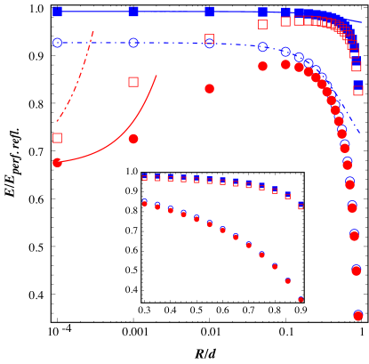
Figure 1: $E/E_{\rm perf.refl.}$ against $R/d$ for the plasma model for $\lambda_{p}/R=0.5$, $0.05$ (open circles and filled squares respetively), and the Drude model for the same values of $\lambda_{p}/R$ (filled circles and open squares, respectively) and $\lambda_{p}/\lambda_{\sigma}=27.4$. The solid and dashed lines represent the asymptotic results of Eqs. (19), (24) for the plasma and the Drude model, respectively. Inset: Magnification of the short distance range.

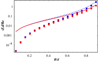
Figure 2: Numerical result for $-Ed/\hbar c$ against $R/d$ for the plasma model at $\lambda_{p}/R=0.05$ (squares) and at $\lambda_{p}/R=0.5$ (circles). The lines represent the PFA energy at $\lambda_{p}/R=0.05$ (dashed) and at $\lambda_{p}/R=0.5$ (solid).

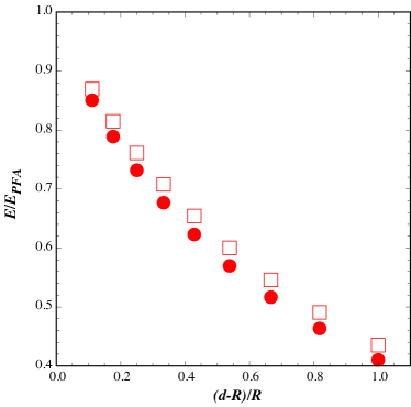
Figure 3: Ratio of the numerical results for the Casimir energy shown in Fig. 2 and the PFA energy based on the Lifshitz theory for the plasma model with $\lambda_{p}/R=0.05$ (squares) and $\lambda_{p}/R=0.5$ (circles). The ratio is shown as a function of the surface-to-surface distance $d-R$.

V.2 Casimir interaction at $T\neq 0$

The Casimir free energy at finite temperatures $T$ depends on the thermal wavelength $\lambda_{T}=\hbar c/k_{B}T$. This additional length scale introduces an additional dimensionless parameter $\lambda_{T}/R$. To investigate the influence of temperature, we calculated the Casimir free energy at two different values of this parameter. We have chosen the values $\lambda_{T}/R=1.52$, $5.94$ since they correspond, e.g., to a sphere of radius $R=5\mu m$, which is small but still relevant to experiments. The temperature is chosen as $T=300^{\circ}K$ and $T=77^{\circ}K$, yielding $\lambda_{T}=7.6\mu$m and $\lambda_{T}=29.7\mu$m, respectively. These two temperatures, corresponding to room temperature and the boiling point of molecular nitrogen N₂ respectively, can readily be accessed in experiments.

Below, we employ more detailed models for the material response to calculate the Casimir energies at higher temperatures. More specifically, we consider generalized plasma and Drude models, which take into account the interband transitions of core electrons that are described by a set of oscillators with nonzero resonant frequencies. The generalized plasma model has the dielectric permittivity

$$\epsilon_{p}(ic\kappa)=1+\left(\frac{2\pi}{\lambda_{p}\kappa}\right)^{2}+\epsilon_{c}(ic\kappa)$$ (32)

and the generalized Drude is described by

$$\epsilon_{p}(ic\kappa)=1+\frac{(2\pi)^{2}}{(\lambda_{p}\kappa)^{2}+\pi c\kappa/\sigma_{p}}+\epsilon_{c}(ic\kappa)$$ (33)

with

$$\epsilon_{c}(ic\kappa)=\sum_{j=1}^{K}\frac{f_{j}}{\omega_{j}^{2}+(c\kappa)^{2}+g_{j}c\kappa}$$ (34)

Here $K$ is the number of oscillators, $f_{j}$ are the oscillator strengths, $g_{j}$ are the relaxation frequency and $\omega_{j}\neq 0$ are the resonant frequencies of the core electrons. Typical parameters for gold are given by $\omega_{p}=9$eV for the plasma frequency and $\gamma=35$meV for the relaxation rate Canaguier-Durand et al. (2009). These parameters correspond to the length scales $\lambda_{p}=2\pi c/\omega_{p}=137$nm and $\lambda_{\gamma}=2\pi c/\gamma=35.4\mu$m. For these parameters, the dc conductivity $\sigma=\omega_{p}^{2}/(4\pi\gamma)$ is $184.2$eV, corresponding to the length scale $\lambda_{\sigma}=2\pi c/\sigma=6.7$nm. Note that electron scattering is not described by the usual plasma model. However, as can be seen from Eq. (32), dissipation is included in the generalized plasma model due to the interband transition of core electrons. To calculate the Casimir energy, we use the oscillator parameters of gold which are presented in Table 1. These parameters have been calculated Decca et al. (2007) based on the 6-oscillator model fitted to the tabulated optical data given in Ref. Palik (1985).

$j$	$\omega_{j}\,[eV]$	$g_{j}\,[eV]$	$f_{j}\,[eV^{2}]$
$1$	$3.05$	$0.75$	$7.091$
$2$	$4.15$	$1.85$	$41.46$
$3$	$5.4$	1.0	$2.700$
$4$	$8.5$	$7.0$	$154.7$
$5$	$13.5$	$6.0$	$44.55$
$6$	$21.5$	$9.0$	$309.6$

Table 1: Oscillator parameters for gold. Calculated in Ref. Decca et al. (2007) by fitting 6 oscillators to tabulated optical data Palik (1985).

We first calculated the $n=0$ term of the sum of Eq. (1) analytically, based on the expressions given in Section IV and then calculate the other terms numerically as explained previously. This allows us to calculate the Casimir free energy for very short separations. As explained above, large values of $\ell_{max}$ should be used at short separations but in this limit the numerical evaluation of the determinant in Eq. (1) is cumbersome. This problem disappears as the temperature in increased because then the second Matsubara wave vector $\kappa_{1}$ becomes larger and thus no calculation for too small values of $\kappa>0$ will be necessary. For the purpose of this paper, we calculate the relevant energies for distances as short as $R/d=0.95$ at the two different temperatures using the generalized form of the Drude and the plasma model, see Eqs. (32), (33).

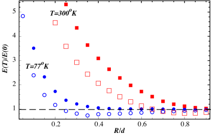
Figure 4: Ratio of the Casimir free energy to the energy at $T=0$ against $R/d$ for the generalized Drude model (open symbols) and the generalized plasma model (filled symbols) at $T=300^{\circ}K$ (squares) and at $T=77^{\circ}K$ (circles) for a sphere of radius $R=5\mu$m.

Fig. 4 shows the ratio of the Casimir free energy to the energy at $T=0$ for the generalized plasma model and for the generalized Drude model at $T=300^{\circ}K$ and $T=77^{\circ}K$. While the Casimir free energy at $T=300^{\circ}K$ is always larger than at $T=77^{\circ}K$ for the plasma model, we find that for the Drude model the Casimir free energies at $T=77^{\circ}K$ and $T=300^{\circ}K$ cross each other around $R/d=0.7$. For $R/d\gtrsim 0.7$, the Casimir free energy corresponding to $T=77^{\circ}K$ becomes larger than the one for $T=300^{\circ}K$. For the sphere plate geometry, indications of negative entropy have recently been reported Canaguier-Durand et al. (2010). The ratio shown in Fig. 4 can be expressed as $E(T)/E(0)=1-TS/E(0)$ where $S$ is the entropy associated with the Casimir free energy $E(T)$. Hence, a ratio $E(T)/E(0)<1$ implies a negative entropy since $E(0)<0$. Our results clearly show that for the Drude model the entropy indeed becomes negative for sufficiently small separations. However, for the plasma model our results of Fig. 4 indicate a positive entropy.

Above we showed that at large separations the ratio of the Casimir energy for the plasma and the Drude model varies between $3/2$ (for small $\lambda_{p}/R$) and $1$ (for large $\lambda_{p}/R$) for zero and finite temperatures. At shorter separations the ratio is expected to tend to one since at high frequencies the plasma and Drude model become identical. It is interesting to observe how the ratio tends to one with decreasing separation as a function of temperature. Fig. 5 shows the Casimir free energy for the plasma model divided by that for the Drude model at $T=300^{\circ}K$, $T=77^{\circ}K$ and $T=0^{\circ}K$. Since $\lambda_{p}/R=0.0274$ is small compared to one, the ratio tends to almost $3/2$ at large separations. As shown in the figure, with decreasing separation the ratio drops towards one very fast for $T=0$. However, for $T=300^{\circ}K$ the ratio is larger than $3/2$ for $R/d\lesssim 0.7$, goes through a maximum around $R/d=0.6$ and finally starts dropping to one. The curve for $T=77^{\circ}K$ also displays a slight maximum close to $R/d=0.15$. A similar behavior with an extrema has been observed also in Ref. Canaguier-Durand et al. (2010) for a sufficiently large sphere at $T=300^{\circ}K$. The maxima occur at a distance that approximately corresponds to the thermal wavelength $\lambda_{T}$ with $R/\lambda_{T}=0.66$ and $R/\lambda_{T}=0.17$ for $T=300^{\circ}K$ and $T=77^{\circ}K$, respectively. Since thermal photons of wavelength $\lambda_{T}$ mostly contribute to the energy at a separation $d\approx\lambda_{T}$, the position of the maxima suggests that thermal effects less strongly enhance the Drude energy than the plasma energy, presumably due to dissipation.

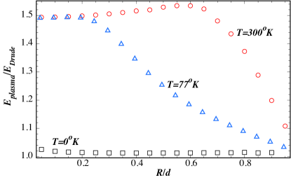
Figure 5: The ratio of Casimir free energies for the generalized plasma and generalized Drude model at $T=300^{\circ}K$ (circles), $T=77^{\circ}K$ (triangles) and $T=0$ (squares).

VI Conclusion

We have shown in detail how the scattering approach for Casimir interactions can be applied to study correlations between effects due to geometry, material properties and finite temperature. The experimentally most relevant geometry of a sphere and plate reveals interesting properties of the Casimir interaction that are absent for parallel plates and hence in the proximity force approximation. These findings demonstrate an interplay between material properties and the finite size of the sphere. Our main results are as follows. At large separations we observe both at zero and finite temperatures for the amplitude of the leading term of the energy different results for perfect reflectors, Drude and plasma metals. The plasma model yields a non-universal amplitude that depends on the ratio of plasma wavelength to sphere radius. For the perfect reflector and Drude model the amplitudes are universal but for the latter it is reduced by a factor of $2/3$. This result is distinct from the interaction of two parallel plates, which at zero temperature is asymptotically identical for the three material descriptions. The identification of the plasma wavelength with the penetration depth of a London superconductor explains why the plasma model yields the asymptotic interaction for perfect reflectors and a Drude metals as limiting cases.

Our numerical computations of the energy at smaller separations demonstrate further important differences between the plasma and Drude model and generalizations thereof. We observe full agreement of the numerical results with the asymptotic expansion at large separations that, however, is limited for the Drude model to extremely large distances. Hence, we conclude that for the Drude model higher order multipoles are more important than for the plasma model. At small separations the observed dependence of the difference between the exact and the PFA energies on the plasma wavelength demonstrates that geometry and material effects are correlated. Our results at finite temperatures show that the Casimir energy for Drude metals changes non-monotonically with temperature, leading to a larger energy at $T=77^{\circ}$K than at $T=300^{\circ}$K at sufficiently small separations. We observe a negative entropy associated with the Casimir free energy for the Drude model over a range of distances. This range increases when the temperature is decreased. Both non-monotonic temperature dependence and negative entropy are not observed for the plasma model in the range of studied parameters. At finite temperatures, we find that the Casimir free energy for plasma metals is approximately $3/2$ times the energy for Drude metals for separations $d\gtrsim\lambda_{T}$.