Factorization in exclusive quarkonium production

Abstract

We present factorization theorems for two exclusive heavy-quarkonium production processes: production of two quarkonia in $e^{+}e^{-}$ annihilation and production of a quarkonium and a light meson in $B$-meson decays. We describe the general proofs of factorization and supplement them with explicit one-loop analyses, which illustrate some of the features of the soft-gluon cancellations. We find that violations of factorization are generally suppressed relative to the factorized contributions by a factor $v^{2}m_{c}/Q$ for each $S$-wave charmonium and a factor $m_{c}/Q$ for each $L$-wave charmonium with $L>0$. Here, $v$ is the velocity of the heavy quark or antiquark in the quarkonium rest frame, $Q=\sqrt{s}$ for $e^{+}e^{-}$ annihilation, $Q=m_{B}$ for $B$-meson decays, $\sqrt{s}$ is the $e^{+}e^{-}$ center-of-momentum energy, $m_{c}$ is the charm-quark mass, and $m_{B}$ is the $B$-meson mass. There are modifications to the suppression factors if quantum-number restrictions apply for the specific process.

I Introduction

A crucial step in the calculation of the amplitudes for hard-scattering hadronic processes is the separation of the effects of the strong interactions into short-distance and long-distance contributions. The short-distance contributions are, by virtue of asymptotic freedom in quantum chromodynamics (QCD), perturbatively calculable, while the long-distance contributions are parametrized in terms of inherently nonperturbative quantities. These separations are usually embodied in factorization theorems for the processes. In the case of hard-scattering processes that involve heavy-quarkonium states, it has been proposed that the effective theory nonrelativistic QCD (NRQCD) could be used to describe the separation of perturbative effects that produce a heavy-quark pair from the nonperturbative effects that bring about the evolution of the heavy-quark pair into the quarkonium bound state Bodwin:1994jh . Recently, progress has been made in understanding factorization issues in inclusive heavy-quarkonium production processes Nayak:2005rt ; Nayak:2005rw ; Nayak:2007mb ; Nayak:2007zb . However, a proof of factorization to all orders in QCD perturbation theory is still lacking for inclusive quarkonium production. In the present paper we discuss factorization for exclusive quarkonium production.

The exclusive production of double-charmonium states in $e^{+}e^{-}$ annihilation has provided an important testing ground in which to compare predictions of theoretical models of charmonium production with experimental measurements. Measurements of the cross sections for double-charmonium production by the Belle Abe:2004ww and BABAR Aubert:2005tj collaborations have, in several instances, disagreed with theoretical predictions Braaten:2002fi ; Liu:2002wq ; Hagiwara:2003cw ; Bodwin:2007ga and have led to a re-examination of the bases for those predictions.

The exclusive decays of $B$ mesons into a light meson plus a charmonium state are also of interest, partly because they could provide new constraints on the Cabibbo-Kobayashi-Maskawa (CKM) matrix and enhance our understanding of the origins of CP violation. However, the nonperturbative effects of the strong interactions are significant in such processes and must be taken into account in order to make reliable QCD-based calculations of the process rates. Factorization theorems for these processes would provide a first-principles framework within which to take into account the strong-interaction effects. In the case of exclusive decays of $B$ mesons into a light meson plus a charmonium state, several factorization theorems have been proposed Beneke:2000ry ; Chay:2000xn ; Bobeth:2007sh .

In this paper, we present proofs, valid to all orders in QCD perturbation theory, of factorization theorems for the exclusive quarkonium-production processes mentioned above, giving details of the proofs that were summarized in Ref. Bodwin:2008nf . These are the first proofs of factorization theorems for quarkonium production. We also present explicit calculations at one-loop order that illustrate key features of the general arguments. Although our analyses are for the specific cases of $B$ decays and $e^{+}e^{-}$ annihilation, the techniques that we describe should apply to other exclusive quarkonium-production processes, and may also shed light on factorization in inclusive quarkonium production. However, we note that, because we consider exclusive two-body quarkonium-production processes, rather than inclusive quarkonium production, we avoid the issues raised in Ref. Nayak:2005rw ; Nayak:2005rt concerning light particles that are comoving with a quarkonium and the issues raised in Ref. Nayak:2007mb ; Nayak:2007zb concerning the color-transfer-enhancement mechanism that appears when an additional heavy quark is comoving with a quarkonium.

In the analysis of Ref. Bodwin:2008nf , it was assumed that gluons cannot have transverse momentum components that are smaller than the QCD scale, $\Lambda_{\rm QCD}$. The possibility that external on-shell lines can emit gluons of arbitrarily low energy was discussed in detail in Ref. Bodwin:2009cb , and it will be considered here as well. The factorization theorems stated in Ref. Bodwin:2008nf remain unchanged.

In the case of the exclusive production of double-charmonium states in $e^{+}e^{-}$ annihilation, we will argue that the production amplitude can be written in the following factorized form:

$$\mathcal{A}\left(e^{+}e^{-}\to\gamma^{*}\to H_{1}+H_{2}\right)=\sum_{ij}A_{ij}\left<H_{1}|\mathcal{O}_{i}|0\right>\left<H_{2}|\mathcal{O}_{j}|0\right>.$$ (1)

The factors $\left<H_{n}|\mathcal{O}_{i}|0\right>$ are NRQCD matrix elements, which describe the nonperturbative evolution of the charm-quark and the charm-antiquark ($c\bar{c}$) pair into a charmonium state $H_{n}$. The sum over the matrix elements is organized as an expansion in powers of $v$, the relative velocity between the $c$ and the $\bar{c}$ in the charmonium rest frame. (For charmonium, $v^{2}\approx 0.3$.) The quantity $A_{ij}$ is a short-distance coefficient, which contains the amplitude for an $e^{+}e^{-}$ pair to annihilate through a virtual photon into two $c\bar{c}$ pairs in the color and angular-momentum states of the NRQCD operators $\mathcal{O}_{i}$ and $\mathcal{O}_{j}$.

In the case of $e^{+}e^{-}$ annihilation, we define the hard-scattering scale $Q\equiv\sqrt{s}$ to be the center-of-momentum (CM) energy of the $e^{+}e^{-}$ pair. We will argue that the factorized form in Eq. (1) holds up to corrections of relative order $f_{1}f_{2}$, where $f_{l}=v^{2}m_{c}/Q$ for an $S$-wave charmonium $H_{l}$, $f_{l}=m_{c}/Q$ for an $L$-wave charmonium $H_{l}$ with $L>0$, and $m_{c}$ is the charm-quark mass. As we will discuss in detail, these suppression factors are modified if quantum-number restrictions apply for the specific process.

In the case of exclusive decays of $B$ mesons into a light meson plus a charmonium state, we will argue that the decay amplitude can be written in the following factorized form:

$$\mathcal{A}\left(B\to H_{1}+K\right)=\sum_{ife}F^{B\to K}_{f(i,e)}(M_{1}^{2})A_{ie}\langle H_{1}|\mathcal{O}_{i}|0\rangle+\sum_{ije}A^{\prime}_{ije}\otimes\Phi_{Kj}\otimes\Phi_{B1}\langle H_{1}|\mathcal{O}_{i}|0\rangle.$$ (2)

Again, the factors $\left<H_{1}|\mathcal{O}_{i}|0\right>$ are the NRQCD matrix elements, which describe the nonperturbative evolution of the $c\bar{c}$ pair into a charmonium state $H_{1}$. The quantities $F_{f}^{B\to K}$, $\Phi_{Kj}$, and $\Phi_{B1}$ are also nonperturbative objects, which we describe below. The quantities $A_{ie}$ and $A^{\prime}_{ije}$ are short-distance coefficients. They contain the amplitude for the electroweak vertex to produce a $c\bar{c}$ pair in the color and angular-momentum state of $\mathcal{O}_{i}$. We approximate the electroweak vertex as a local four-fermion vertex. The sum over $e$ is over the various operators in the electroweak effective action. The sum over $f$ is over the allowed form factors that result from shrinking the hard subdiagram (to be described later) to a local vertex with respect to the $B$-meson-to-light-meson transition process. The symbol $\otimes$ represents the convolution of a short-distance coefficient with the light-cone distributions of the light meson and the $B$ meson.

The first term of Eq. (2) contains a $B$-meson-to-light-meson form factor

$$F^{B\to K}_{f(i,e)}(M_{1}^{2})=\langle K|\bar{\Psi}_{l}\Gamma_{f(i,e)}\Psi_{b}|B\rangle.$$ (3)

Here, $B$ and $K$ denote the $B$ meson and the light meson, respectively, and $M_{1}$ is the charmonium mass. The quantity $\Gamma_{f(i,e)}$ is the product of a Dirac matrix and a color matrix that arises when one shrinks the hard-scattering subdiagram to a point with respect to the $B$-meson-to-light-meson transition amplitude. It is understood that the fields $\bar{\Psi}_{l}$ and $\Psi_{b}$ are in a color-singlet state. Following Ref. Beneke:2000ry , we define $F_{f}^{B\to K}$ in the first term in Eq. (2) to be the “physical” meson form factor, which contains both hard and soft contributions. Then, in the second term in Eq. (2), one must omit from the short-distance coefficients the hard contributions that are already contained in the first term in Eq. (2).

The second term of Eq. (2) involves the light-cone distribution amplitude(s) of the light meson $\Phi_{Kj}$, which are defined by the expression

$$\frac{p_{K}^{-}}{\pi}\int_{-\infty}^{+\infty}dx^{+}{\rm exp}[-i(2y-1)p_{K}^{-}x^{+}]\langle K(p_{K})|\bar{\Psi}_{\alpha}(x^{+})P[x^{+},-x^{+}]\Psi_{\beta}(-x^{+})|0\rangle$$

$$\quad\quad\equiv\sum_{j}\Phi_{Kj}(y)\left[\Gamma_{Kj}\right]_{\alpha\beta},$$ (4)

and the light-cone distribution of the $B$ meson $\Phi_{B1}$, which is defined by the expression

$$\frac{p_{B}^{+}}{2\pi}\int_{-\infty}^{+\infty}dx^{-}{\rm exp}[i\xi p_{B}^{+}x^{-}]\langle 0|\bar{\Psi}_{l\beta}(x^{-})P[x^{-},0]\Psi_{b\alpha}(0)|B(p_{B})\rangle$$

$$\quad\quad\equiv\sum_{m}\Phi_{Bm}(\xi)\left[\Gamma_{Bm}\right]_{\alpha\beta}$$

$$\quad\quad\approx-\frac{if_{B}}{4}\left\{(/\!\!\!p_{b}+m_{b})\gamma_{5}\left[\Phi_{B1}(\xi)+/\!\!\!n_{-}\Phi_{B2}(\xi)\right]\right\}_{\alpha\beta}.$$ (5)

Here, $\Psi$ is the quark field, $\alpha$ and $\beta$ are Dirac indices, $\bar{\Psi}$ and $\Psi$ in each matrix element are understood to be in a color-singlet state, and the $\Gamma_{Kj}$ and the $\Gamma_{Bm}$ are Dirac-matrix structures for the light meson and the $B$ meson, respectively. We define light-cone variables $k=(k^{+},k^{-},\bm{k}_{\perp})$ in terms of Cartesian components as $k^{+}=(1/\sqrt{2})(k^{0}+k^{z})$ and $k^{-}=(1/\sqrt{2})(k^{0}-k^{z})$. In Eq. (I), $n_{-}$ is the vector $n_{-}=\sqrt{2}(0,1,\bm{0}_{\perp})$, and we have retained only the leading-twist $B$ meson light-cone distributions. We take the spatial components of $p_{K}$ to lie along the minus $z$ direction, and we take the $B$ meson to be at rest. The expression $[y,x]$ in Eqs. (I) and (I) is the exponentiated line integral of the gauge field:

$$[y,x]=\exp\left[\int_{x}^{y}igT_{a}A_{\mu}^{a}dx^{\mu}\right].$$ (6)

$P$ indicates path ordering, $T_{a}$ is a generator of color SU(3), and $A_{\mu}^{a}$ is the gluon field.

In the case of $B$-meson decays, we define the hard-scattering scale $Q$ to be the $B$-meson mass $m_{B}$. We will argue that the factorized form in Eq. (2) holds up to corrections of relative order $f_{1}$, where $f_{1}=v^{2}m_{c}/Q$ for an $S$-wave quarkonium $H_{1}$ and $f_{1}=m_{c}/Q$ for an $L$-wave quarkonium $H_{1}$ with $L>0$. As in the $e^{+}e^{-}$-annihilation case, these suppression factors are modified if quantum-number restrictions apply for the specific process. This result was suggested previously in Ref. Beneke:2000ry . However, there it was conjectured only that the violations of factorization vanish in the limit $m_{c}\to 0$.

The remainder of this paper is organized as follows. In Sec. II, we specify models for the production amplitudes. In Sec. III, we outline the proofs of factorization for the processes under consideration. There we describe the momentum regions that are leading in the hard-scattering scale, the momentum regions in which loop integrands become singular, the diagrammatic topologies of the leading and singular regions, the approximations that are appropriate to contributions involving momenta that are soft or collinear, the factorization of the soft and collinear singular regions, the subsequent construction of the factorized form, and the corrections to the factorized form. We illustrate general features of the factorization proof with explicit one-loop examples in Sec. IV. In Sec. IV.1 we describe the implementation of the soft approximation at the one-loop level. Sections IV.2 and IV.3 contain one-loop examples for $e^{+}e^{-}$ annihilation and $B$ decays, respectively. We summarize and discuss our results in Sec. V. The Appendix contains the expressions for the quark-antiquark spin-projection operators that we use in Sec. IV.

II Model for the amplitude

We carry out our analyses in the rest frame of the $B$ meson and in the CM frame of the $e^{+}e^{-}$ pair, choosing the three-momentum of the quarkonium $H_{1}$ to be in the positive $z$ direction and choosing the three-momentum of the light meson $K$ or the quarkonium $H_{2}$ to be in the negative $z$ direction. We take the constituents of each meson and quarkonium to be on the mass shell. We also assume that, for each meson and quarkonium, there is an integration over the relative momentum of the constituents, weighted by a meson wave function, and subject to the mass-shell constraints.

We model the $B$ meson as an on-shell “active” bottom quark, which participates in the electroweak interaction, and an on-shell “spectator” light antiquark, which does not participate in the electroweak interaction. We take the quark and antiquark to be in a color-singlet state. We take the bottom quark to have momentum $p_{b}$ and mass $m_{b}$, with (in Cartesian coordinates)

$$p_{b}=\left(\sqrt{m_{b}^{2}+\bm{q}_{B}^{2}},\bm{q}_{B}\right)\sim\left(m_{b},\Lambda_{\rm QCD}\right).$$ (7)

We take the spectator antiquark to have momentum $p_{l}$, with

$$p_{l}=\left(|\bm{q}_{B}|,-\bm{q}_{B}\right)\sim\left(\Lambda_{\rm QCD},\Lambda_{\rm QCD}\right).$$ (8)

The momentum of the $B$ meson, $p_{B}$, is given by the sum of $p_{b}$ and $p_{l}$:

$$p_{B}=p_{b}+p_{l}=\left(m_{B},\bm{0}\right)=\left(\sqrt{m_{b}^{2}+\bm{q}_{B}^{\;2}}+|\bm{q}_{B}|,\bm{0}\right)\sim\left(m_{b},\bm{0}\right).$$ (9)

Similarly, we model the light meson $K$ as an on-shell active light quark and an on-shell spectator light antiquark, with the quark and antiquark in a color-singlet state. We can write the quark momentum, $p_{k_{q}}$, and the antiquark momentum, $p_{k_{\bar{q}}}$, as

$$p_{k_{q}} = \frac{1}{2}p_{K}+r_{k},$$ (10a)

$$p_{k_{\bar{q}}} = \frac{1}{2}p_{K}-r_{k},$$ (10b)

with $p_{K}\cdot r_{k}=0$. In the rest frame of the light meson, we denote the vectors that are associated with the light meson with a hat. Then, we have

$$\hat{p}_{K} = \left(m_{K},\bm{0}\right)=\left(2|\hat{\bm{r}}_{k}|,\bm{0}\right),$$ (11a)

$$\hat{r}_{k} = (0,\hat{\bm{r}}_{k}),$$ (11b)

$$\hat{p}_{k_{q}} = \left(|\hat{\bm{r}}_{k}|,\hat{\bm{r}}_{k}\right),$$ (11c)

$$\hat{p}_{k_{\bar{q}}} = \left(|\hat{\bm{r}}_{k}|,-\hat{\bm{r}}_{k}\right).$$ (11d)

The quantity $\hat{\bm{r}}_{k}$ is of order $\Lambda_{\rm QCD}$.

The boosts from the light-meson rest frame to the $B$-meson rest frame are given, for an arbitrary momentum $k$, by

$$\hat{k}^{+} \to \frac{E_{K}-P_{\rm CM}}{m_{K}}\,\hat{k}^{+},$$ (12a)

$$\hat{k}^{-} \to \frac{E_{K}+P_{\rm CM}}{m_{K}}\,\hat{k}^{-},$$ (12b)

$$\hat{k}_{\perp} \to \hat{k}_{\perp}.$$ (12c)

Here, $P_{\rm CM}$ is the magnitude of the three-momentum of either $H_{1}$ or $K$ in the $B$-rest frame,

$$P_{\rm CM} = \frac{\lambda^{1/2}(s,M_{1}^{2},m_{K}^{2})}{2\sqrt{s}}\sim m_{b}\;,$$ (13a)

$$\lambda(x,y,z) = x^{2}+y^{2}+z^{2}-2(xy+yz+zx)\;,$$ (13b)

$E_{K}$ is the energy of the meson $K$,

$$E_{K}=\sqrt{P_{\rm CM}^{2}+m_{K}^{2}}\sim m_{b}\;.$$ (14)

$M_{1}\sim m_{c}$ in Eq. (13a) is the heavy-quarkonium mass, which we will define in our model below. Therefore, in the $B$-meson rest frame we have

$$p_{K} = \left(\frac{1}{\sqrt{2}}\left[E_{K}-P_{\rm CM}\right],\frac{1}{\sqrt{2}}\left[E_{K}+P_{\rm CM}\right],\bm{0}_{\perp}\right)\sim\left(\frac{\Lambda_{\rm QCD}^{2}}{m_{b}},m_{b},\bm{0}_{\perp}\right),$$ (15a)

$$r_{k} = \left(\frac{\hat{r}_{k}^{z}}{\sqrt{2}}\,\frac{E_{K}-P_{\rm CM}}{m_{K}},-\frac{\hat{r}_{k}^{z}}{\sqrt{2}}\,\frac{E_{K}+P_{\rm CM}}{m_{K}},\hat{\bm{r}}_{k\perp}\right)\sim\left(\frac{\Lambda_{\rm QCD}^{2}}{m_{b}},m_{b},\Lambda_{\rm QCD}\right).$$ (15b)

It is now convenient to define a momentum fraction $y$ and a vector $q_{k}$ that has zero minus component. In terms of these quantities, the momenta of the quark and the antiquark are

$$p_{k_{q}} = yp_{K}+q_{k},$$ (16a)

$$p_{k_{\bar{q}}} = (1-y)p_{K}-q_{k}\equiv\bar{y}p_{K}-q_{k}.$$ (16b)

$y$ is the fraction of minus component of the momentum of the meson that is carried by the quark:

$$y=\frac{1}{2}+\frac{r_{k}^{-}}{p_{K}^{-}}.$$ (17)

Hence,

$$q_{k}=\left(\frac{1}{2}-y\right)p_{K}+r_{k}=\left(2\frac{\hat{r}_{k}^{z}}{\sqrt{2}}\,\frac{E_{K}-P_{\rm CM}}{m_{K}},0,\hat{\bm{r}}_{k\perp}\right)\sim\left(\frac{\Lambda_{\rm QCD}^{2}}{m_{b}},0,\Lambda_{\rm QCD}\right).$$ (18)

Finally, we model the charmonium states as an on-shell charm quark and an on-shell charm antiquark in a color-singlet state, with the momentum of the charm quark equal to $p_{iq}$ and the momentum of the charm antiquark equal to $p_{i\bar{q}}$. We take

$$p_{iq} = \frac{1}{2}P_{i}+q_{i},$$ (19a)

$$p_{i\bar{q}} = \frac{1}{2}P_{i}-q_{i},$$ (19b)

where $P_{i}$ is the quarkonium momentum and $P_{i}\cdot q_{i}=0$. In the quarkonium rest frame, we denote vectors that are associated with the quarkonium with a hat. The quantity $\hat{q}_{i}$ has only spatial components, whose magnitudes are of order $m_{c}v$. Hence,

$$\hat{P}_{i} = (M_{i},\bm{0})=\left(2\sqrt{m_{c}^{2}+\hat{\bm{q}}_{i}^{2}},\bm{0}\right),$$ (20a)

$$\hat{q}_{i} = (0,\hat{\bm{q}}_{i}).$$ (20b)

In the case in which the quarkonium $i$ is in a spin-triplet state, we also define a spin-polarization vector $\epsilon_{i}$. In the quarkonium $i$ rest frame, $\epsilon_{i}$ has spatial components of order unity and temporal component zero:

$$\hat{\epsilon}_{i}=(0,\hat{\bm{\epsilon}}_{i}),$$ (21)

which implies that $P_{i}\cdot\epsilon_{i}=0$.

The boost from the rest frame of the quarkonium with momentum $P_{1}$ to the $B$-meson rest frame or the $e^{+}e^{-}$ CM frame is

$$\hat{k}^{+} \to \frac{E_{1}+P_{\rm CM}}{M_{1}}\,\hat{k}^{+},$$ (22a)

$$\hat{k}^{-} \to \frac{E_{1}-P_{\rm CM}}{M_{1}}\,\hat{k}^{-},$$ (22b)

$$\hat{k}_{\perp} \to \hat{k}_{\perp}.$$ (22c)

The boost from the rest frame of the quarkonium with momentum $P_{2}$ to the $e^{+}e^{-}$ CM frame is

$$\hat{k}^{+} \to \frac{E_{2}-P_{\rm CM}}{M_{2}}\,\hat{k}^{+},$$ (23a)

$$\hat{k}^{-} \to \frac{E_{2}+P_{\rm CM}}{M_{2}}\,\hat{k}^{-},$$ (23b)

$$\hat{k}_{\perp} \to \hat{k}_{\perp}.$$ (23c)

Here,

$$E_{i} = \sqrt{P_{\rm CM}^{2}+M_{i}^{2}}\sim Q\;,$$ (24a)

$$P_{\rm CM} = \frac{\lambda^{1/2}(s,M_{1}^{2},\widetilde{M}_{2}^{2})}{2\sqrt{s}}\sim Q\;,$$ (24b)

$$M_{i} = 2\sqrt{m_{c}^{2}+\hat{\bm{q}}_{i}^{2}}.$$ (24c)

$\widetilde{M}_{2}=M_{2}$ in the case of $e^{+}e^{-}$ annihilation into two quarkonia, and $\widetilde{M}_{2}=m_{K}$ in the case of $B$-meson decays. It then follows that, in the $e^{+}e^{-}$ CM frame or the $B$-meson rest frame,

$$\begin{array}[]{lcl}P_{1}^{+}\sim Q,&&P_{2}^{+}=2\frac{m_{c}^{2}-q_{2}^{2}}{P_{2}^{-}}\sim\frac{m_{c}^{2}}{Q},\\ P_{1}^{-}=2\frac{m_{c}^{2}-q_{1}^{2}}{P_{1}^{+}}\sim\frac{m_{c}^{2}}{Q},&&P_{2}^{-}\sim Q,\\ {\bm{P}}_{1\perp}=0,&&{\bm{P}}_{2\perp}=0,\\ q_{1}^{+}\sim vQ,&&q_{2}^{+}\sim\frac{vm_{c}^{2}}{Q},\\ q_{1}^{-}\sim\frac{vm_{c}^{2}}{Q},&&q_{2}^{-}\sim vQ,\\ \epsilon_{1}^{+}\sim\frac{Q}{m_{c}},&&\epsilon_{2}^{+}\sim\frac{m_{c}}{Q},\\ \epsilon_{1}^{-}\sim\frac{m_{c}}{Q},&&\epsilon_{2}^{-}\sim\frac{Q}{m_{c}},\\ \bm{q}_{i\perp}\sim m_{c}v,&&\bm{\epsilon}_{i\perp}\sim 1.\end{array}$$ (25)

III Proof of factorization

III.1 Strategy

If we dress the lowest-order decay and production amplitudes in our models with additional gluons, then certain regions of integration of the gluon momenta yield contributions that are leading in powers of the large momentum scale, $Q$. We will describe these regions in Sec. III.2 below. We wish to isolate the contributions from the loop integrations that can be calculated in perturbation theory from those that cannot. That is, we wish to isolate contributions in which propagators have large virtuality, of order $Q$, from contributions with lower virtualities. We call the large-virtuality part of the amplitude the “hard” part. In order to establish factorization, we will show that the low-virtuality contributions either cancel or can be absorbed into nonperturbative functions. The nonperturbative functions are the NRQCD matrix elements for the charmonia and, in the case of $B$-meson decays, the $B$-meson-to-light-meson form factor, the light-cone distribution amplitude for the $B$ meson, and the light-cone distribution amplitude for the light meson. We will first demonstrate a factorization involving quarkonium distribution amplitudes. Then, we will argue that the distribution amplitudes can be straightforwardly decomposed into a sum over NRQCD matrix elements multiplied by short-distance coefficients. After the factorization of low-virtuality contributions, the remaining hard part will depend only on the momenta and spins of the quarks and antiquarks that enter into the leading-order process and will be independent of the low-virtuality properties of the external mesons.

The low-virtuality contributions arise from regions of loop integration that are logarithmically enhanced. In these logarithmically enhanced regions, loop integrations have logarithmic power counts and can lead to actual infrared (IR) divergences or would-be IR divergences that are cut off by scales smaller than $Q$, such as quark masses. In the case of a would-be divergence that arises from the emission of a gluon that is nearly collinear to one of the external charm quarks, the minimum virtuality of the quark propagator is of order $m_{c}^{2}|\bm{k}|/(2|\bm{p}|)$, where $k$ is the gluon momentum and $p$ is the charm-quark momentum. Hence, the virtuality can be much less than $Q^{2}$, and even of order $\Lambda_{\rm QCD}^{2}$. Therefore, we must factor such contributions from the hard part in order to arrive at a perturbatively calculable contribution.

One could, in principle, deal with the low-virtuality contributions by devising a suitable subtraction scheme for the contributions that would appear order by order in perturbation theory. That would be a formidable task, as one would need to ensure that all such contributions are accounted for in an arbitrarily complicated Feynman diagram, with no double counting of contributions.

For our purposes, we can take a simpler approach. We consider the singularities that appear in the limit $m_{c}\to 0$ with $q_{i}$ fixed. First, we establish that the contributions from infinitesimal neighborhoods of these singularities can be factored into nonperturbative functions. Then, we restore $m_{c}$ to its physical value and extend the regions contained in the nonperturbative functions from the infinitesimal neighborhoods of the singularities to regions of finite size. Then the hard part, which is defined to be the remainder of the amplitude, contains no logarithmically enhanced contributions.

The factorization proofs entail the use of soft and collinear approximations, which are exact at the singular points. These approximations are described in Secs. III.5 and III.6. The actual factorization is achieved through the use of decoupling relations, which are based on the graphical Ward identities of QCD. These decoupling relations are described in Sec. III.7.

We note that, because our models make use of on-shell external quarks and antiquarks, it is possible to emit collinear and nearly collinear gluons of arbitrarily low energy from the external lines. This situation is discussed in detail in Ref. Bodwin:2009cb . It is unphysical since, in a meson, confinement cuts off gluon energies at values of order $\Lambda_{\rm QCD}$. Nevertheless, it is important to establish factorization in the on-shell case in order to guarantee the consistency of perturbative calculations of the hard part, which are usually carried out in the context of on-shell amplitudes. Because the logarithmically enhanced contributions in the presence of a cutoff of order $\Lambda_{\rm QCD}$ are a subset of the logarithmically enhanced contributions in the case of on-shell external lines, the factorization argument that we will present also applies in the simpler case of a model with a cutoff. As we will see, the methods that we use to prove factorization apply to models in which the external particles are off their mass shells, provided that the models maintain gauge invariance. For example, one could model the $B$ meson as an elementary, color-singlet pseudoscalar that produces the constituent quark and antiquark off their mass shells through a pointlike pseudoscalar-interaction vertex that is proportional to $\gamma_{5}$.

III.2 Leading momentum regions

In describing the regions of loop momenta that yield contributions that are leading in powers of the large scale $Q$, we make use of the nomenclature of Ref. Bodwin:2009cb . We first describe the various regions of momentum space, and then, in Sec. III.2.5, we specify the conditions that must be fulfilled in order for these regions to give leading contributions to an amplitude. In a Feynman diagram, we call a gluon or quark, or, generically, a line that carries momentum of type $X$ an “$X$ gluon,” “$X$ quark,” or “$X$ line.”

III.2.1 Hard, soft, and collinear regions

The hard ($H$), soft ($S$), collinear-to-plus ($C^{+}$), and collinear-to-minus ($C^{-}$) momenta have components with the following orders of magnitude:

$$H:\,\,\, Q(1,1,\bm{1}_{\perp}),$$ (26a)

$$S:\,\,\,\, Q\epsilon_{S}(1,1,\bm{1}_{\perp}),$$ (26b)

$$C^{+}: Q\epsilon^{+}[1,(\eta^{+})^{2},\bm{\eta}^{+}_{\perp}],$$ (26c)

$$C^{-}: Q\epsilon^{-}[(\eta^{-})^{2},1,\bm{\eta}^{-}_{\perp}].$$ (26d)

The energy scales of the various types of momenta are determined by the parameters $\epsilon_{S}$, $\epsilon^{+}$, and $\epsilon^{-}$. The soft region of momentum space is defined by the condition

$$\epsilon_{S}\ll 1.$$ (27)

The collinear regions of momentum space are defined by the conditions

$$\epsilon^{\pm} \lesssim 1,$$

$$\eta^{\pm} \ll 1.$$ (28)

In the case of $B$-meson decays, there is also a leading region that is associated with momenta that are nearly collinear to the light-quark momentum $p_{l}$. We call this region $C^{l}$. It is characterized by momenta that scale as

$$C^{l}:\,\,\,Q\epsilon^{l}[{e}_{l}+(\eta^{l})^{2}\bar{e}_{l}+\eta^{l}e_{l}^{T}],$$ (29)

where ${e}_{l}$, is a unit vector that is parallel to the lightlike vector $p_{l}$, $\bar{e}_{l}$ is the parity inverse of ${e}_{l}$, and $e_{l}^{T}$ is a unit vector that is transverse to $e_{l}$ and $\bar{e}_{l}$. The $C^{l}$ region is defined by

$$\epsilon^{l} \lesssim \Lambda_{\rm QCD}/Q,$$

$$\eta^{l} \ll 1.$$ (30)

We assume that $p_{l}$ does not lie exactly in the plus or minus direction. In order to simplify the discussion to follow, we often do not mention $C^{l}$ momenta explicitly. In these instances, it may be assumed that the lines carrying $C^{l}$ momenta may be treated analogously to the lines carrying $C^{\pm}$ momenta.

We note that soft and collinear contributions lie in restricted regions of phase space. Were it not for enhancements that arise from propagators with low virtuality, soft contributions would be suppressed by a phase-space factor $\epsilon_{S}^{4}$ and collinear contributions would be suppressed by a phase-space factor $(\epsilon^{\pm})^{4}(\eta^{\pm})^{4}$. The low-virtuality propagators associated with these contributions lead to loop integrals that have a logarithmic power count and to contributions that behave as $\epsilon_{S}^{0}$ and $(\epsilon^{\pm})^{0}(\eta^{\pm})^{0}$. We refer to such contributions as soft and collinear logarithmic enhancements.

The definitions given above for the $H$, $S$, and $C^{i}$ momentum regions do not specify unambiguously the boundaries between them. For instance, if the $\eta^{i}$ parameters in the collinear regions take on values that are not too different from one, then the $C^{i}$ momenta are not distinguished from the $S$ momenta; i.e., it would not be clear if a $C^{i}$ momentum with $\eta^{i}$ close to 1 belongs to the $C^{i}$ region or to the $S$ region. Hence, the possibility of double counting arises. Analogous issues appear at the other boundaries between the $H$, $S$, and $C^{i}$ regions. However, as we have mentioned previously, this is not a problem for our proof of factorization, which will be presented later, because the proof focuses on the singularities and would-be singularities, rather than on the momentum regions. The heuristic description of regions presented here is intended only to set the stage for the subsequent discussions of the singular regions.

In contrast with the corresponding momentum regions, the soft and collinear singularities are distinct. The soft singularities appear in the limit $\epsilon_{S}\to 0$ or $\epsilon^{i}\to 0$ and the collinear singularities appear in the limits $\eta^{i}\to 0$. A double (soft and collinear) singularity can arise if $\epsilon^{i}\to 0$ and $\eta^{i}\to 0$ at the same time.

III.2.2 Endpoint region

In the case of $B$-meson decays, there is a leading contribution from the so-called “endpoint” region Beneke:2000ry . This contribution is associated with a gluon that connects the $B$-meson and light-meson antiquarks to the remainder of the amplitude. The contribution in the endpoint region arises from a would-be infrared divergence that corresponds to the singular point at $\bar{y}=0$. The divergence is cut off by $q_{k}$, the residual momentum of light-meson antiquark, and by $p_{l}$, the momentum of the $B$-meson antiquark, both of which are of order $\Lambda_{\rm QCD}$. That is, the divergence is cut off at $\bar{y}\sim\Lambda_{\rm QCD}/m_{b}$. In our model, the explicit diagrammatic factors yield a linearly divergent power count, but the would-be divergence is moderated by a factor $\bar{y}$ from the light-meson wave function and is actually logarithmic. The gluon that is associated with the endpoint region carries $S$ momentum of order $\Lambda_{\rm QCD}$.

If the gluon that is associated with the endpoint region attaches to an active-quark line from the $B$ meson or the light meson or to a heavy-quark or heavy-antiquark line from the charmonium, then its momentum causes the propagators of those lines to be off shell by an amount of order $m_{b}\Lambda_{\rm QCD}$. We call such lines “semihard” lines. Contributions from these lines can be calculated in perturbation theory. We treat the semihard region as part of the hard region, and we include lines carrying semihard momenta in the hard subdiagram that we will describe below.

III.2.3 Glauber region

The “Glauber” region is also leading in power counting Bodwin:1994jh ; Bodwin:1984hc . In this region, $|k^{+}|\ll|k_{\perp}|$, $|k^{-}|\ll|k_{\perp}|$, and $k_{\perp}^{2}\ll Q^{2}$. In processes with two incoming hadrons, such as Drell-Yan lepton-pair production, pinch singularities can develop in the Glauber region for the $k^{+}$ and $k^{-}$ contours of integration on a diagram-by-diagram basis Bodwin:1984hc ; Collins:1985ue ; Collins:1989gx . The pinches arise when a gluon connects a spectator parton in one initial-state hadron with a spectator parton in the other initial-state hadron. (Here, in contrast with the terminology that is used to discuss exclusive $B$-meson decays, “spectator parton” means a parton that does not participate in the hard-scattering process.) The pinches appear because the momentum of a gluon that attaches to a spectator-parton line must route through the hadron wave function and the active-parton line from that hadron to the hard process. If the gluon’s momentum in the active-parton line is in the same direction as the momentum of the active parton, then, in the spectator-parton line, it is in the direction opposite to the momentum of the spectator parton. Consequently, there is a pinch in the light-cone variable that is conjugate to the direction of the momentum of the hadron. In contrast, in exclusive processes, all of the partons in a hadron are connected in the lowest-order process, either through the hard subprocess or, possibly through a soft gluon in the case of $B$-meson decays. (See the discussion of the endpoint region above.) Thus, if an additional gluon carrying soft momentum attaches to a parton, one can always route that momentum through a leading-order connection to the hard part, avoiding routings through other partons in the hadron that could produce a pinch. Because of this, the $k^{+}$ and $k^{-}$ contours of integration are not pinched in the Glauber region in exclusive processes, and it is possible to deform them out of the Glauber region on a diagram-by-diagram basis. Therefore, we ignore the Glauber region in the remainder of our discussion.

III.2.4 Threshold region

In the case of a quarkonium, there are “threshold enhancements” that are associated with the exchange of a gluon between the quark and the antiquark. (See Ref. Bodwin:1994jh for examples.) In the quarkonium rest frame, the enhancement occurs when the exchanged gluon has momentum components $\hat{k}^{0}\sim m_{c}v^{2}$ and $|\hat{\bm{k}}|\sim m_{c}v$. The enhancement produces a power infrared divergence that is cut off by the relative momentum of the quark and antiquark $\hat{\bm{q}}\sim m_{c}v$. The divergence is proportional to $m_{c}/|\hat{\bm{q}}|\sim 1/v$. Now let us consider the momentum of the exchanged gluon in the $e^{+}e^{-}$ CM frame in the case of $e^{+}e^{-}$ annihilation and in the $B$-meson rest frame in the case of $B$-meson decays. In these frames, as can be seen from the boosts in Eqs. (22) and (23), an exchanged gluon in the quarkonium with momentum $P_{1}$ has momentum $k\sim(Qv,m_{c}^{2}v/Q,m_{c}\bm{v}_{\perp})$, and an exchanged gluon in the quarkonium with momentum $P_{2}$ has momentum $k\sim(m_{c}^{2}v/Q,Qv,m_{c}\bm{v}_{\perp})$. Therefore, the exchanged gluons associated with threshold enhancement have $C^{+}$ or $C^{-}$ momentum, and, in our analysis, we do not distinguish them from other gluons with $C^{+}$ or $C^{-}$ momentum. Because the threshold enhancements involve the gluons and heavy quarks in a single quarkonium, in each Feynman diagram they are a priori compatible with the factorized forms. Therefore, it will not be necessary to manipulate the threshold contributions or to identify them by considering the limit $v\to 0$.

III.2.5 Leading momentum configurations in Feynman diagrams

Next we identify the configurations of momentum types that can yield leading contributions in the Feynman diagrams. By “leading”, we mean contributions that are not suppressed as powers of ratios of momentum components. We follow the analysis presented in Ref. Bodwin:2009cb . Here, and throughout this paper, we work in the Feynman gauge.

We start with a basic diagram that is just the amplitude of lowest order that involves the external quark and antiquark from each meson. Then we add gluons, one at a time, determining for each gluon the momentum types that produce leading contributions. The added gluons can contain quark, gluon, and ghost vacuum-polarization loops.

Because there are many redundant ways to obtain a given momentum configuration in a diagram, it is useful to define a convention for the way in which we add gluons. In order to do that, we first define combination momenta $\tilde{C}^{\pm}$ and $CC$. A $\tilde{C}^{\pm}$ momentum arises from the sum of a $C^{\pm}$ momentum and an $S$ momentum with $\epsilon_{S}\sim\epsilon^{\pm}\eta^{\pm}$ or from the sum of a $C^{\pm}$ momentum and a $C^{\mp}$ momenta with $\epsilon^{\pm}(\eta^{\pm})^{2}\ll\epsilon^{\mp}\ll\epsilon^{\pm}$. A $CC$ momentum arises from the sum of a $C^{\pm}$ momentum and a $C^{\mp}$ momentum with $\epsilon^{+}\sim\epsilon^{-}$. These combination momenta have the following orders of magnitude:

$$\tilde{C}^{+}: Q\epsilon^{+}(1,\tilde{\eta}^{+},\bm{\eta}^{+}_{\perp}),$$ (31a)

$$\tilde{C}^{-}: Q\epsilon^{-}(\tilde{\eta}^{-},1,\bm{\eta}^{-}_{\perp}),$$ (31b)

$$CC: Q\epsilon_{CC}(1,1,\bm{\eta}_{CC\perp}),$$ (31c)

where

$$1\gg\tilde{\eta}^{\pm}\gg(\eta^{\pm})^{2}.$$ (32)

Analogous combination momenta may be defined for combinations of $C^{l}$ momenta with other momenta. A $\tilde{C}^{l}$ momentum has dominant component in the $e_{l}$ direction. A $CC^{l}$ momentum, which arises from the sum of a $C^{l}$ momentum and a $C^{\pm}$ momentum with $\epsilon^{l}\sim\epsilon^{\pm}$, has at least two components of order $\epsilon^{l}$.

Now we define our convention for adding gluons to the basic diagram. We say that a gluon with momentum $l$ can attach to a line with momentum $p$ only if the energy scale of the momentum $p+l$ is of the same order as the $\epsilon$ parameter of the momentum $p$ and one of the following conditions is fulfilled:

1. The momentum $p+l$ is of the same type as the momentum $p$;

2. The momentum $p$ is $C^{i}$ and $p+l$ is $\tilde{C}^{i}$;

3. The momentum $p$ is $C^{i}$ or $\tilde{C}^{i}$ and $p+l$ is $CC$.

$k$ $\backslash$ $p$          $S$           $C^{\pm}$           $\tilde{C}^{\pm}$    $S$ $\epsilon_{S_{k}}\sim\epsilon_{S_{p}}$ $\epsilon_{p}^{\pm}(\eta^{\pm}_{p})^{2}\lesssim\epsilon_{S_{k}}\ll\epsilon_{p}^{\pm}$ $\epsilon_{p}^{\pm}\tilde{\eta}_{p}^{\pm}\lesssim\epsilon_{S_{k}}\ll\epsilon_{p}^{\pm}$

$k$ $\backslash$ $p$          $S$          $C^{\mp}$          $\tilde{C}^{\mp}$          $CC$    $C^{\pm}$ $\epsilon^{\pm}_{k}\sim\epsilon_{S_{p}}$ $\epsilon_{p}^{\mp}(\eta^{\mp}_{p})^{2}\lesssim\epsilon^{\pm}_{k}\lesssim\epsilon^{\mp}_{p}$ $\epsilon^{\mp}_{p}\tilde{\eta}^{\mp}_{p}\lesssim\epsilon^{\pm}_{k}\lesssim\epsilon^{\mp}_{p}$ $\epsilon^{\pm}_{k}\sim\epsilon_{{CC}_{p}}$ $CC$ $\epsilon_{CC_{k}}\sim\epsilon_{S_{p}}$ $\epsilon_{p}^{\mp}(\eta^{\mp}_{p})^{2}\lesssim\epsilon_{CC_{k}}\ll\epsilon^{\mp}_{p}$ $\epsilon^{\mp}_{p}\tilde{\eta}^{\mp}_{p}\lesssim\epsilon_{CC_{k}}\ll\epsilon^{\mp}_{p}$ $\epsilon_{CC_{k}}\sim\epsilon_{CC_{p}}$

Table 1: Conditions that a gluon with momentum $k$ must fulfill in order to attach to a line with momentum $p$. These conditions guarantee that the resulting attachment is allowed according to the convention described in the text and that it results in a leading contribution. Here, “leading” means that the contribution is not suppressed as powers of ratios of momentum components. In each table, the left-hand column gives the momentum type of the gluon with momentum $k$, and the top row gives the momentum type of the line with momentum $p$. The symbol “$\sim$” means that quantities are of the same order. For purposes of power counting, an $H$ line behaves as a soft line with $\epsilon_{S}\sim 1$. The rules for attachment when $k$ is $\tilde{C}^{\pm}$ are the same as the rules for attachment when $k$ is $C^{\pm}$. If $k$ is $S$, and the lines to which it attaches have momentum $p_{i}$ and $p_{j}$, then $p_{i}$ and $p_{j}$ cannot both be $C^{+}$ or $C^{-}$. If $k$ is $C^{\pm}$, then at least one of $p_{i}$ and $p_{j}$ is $C^{\pm}$. Analogous conditions exist for the attachments of gluons with $C^{l}$ momenta.

The analysis in Ref. Bodwin:2009cb shows that, if we consider only the terms $2p\cdot l$ in propagator denominators, then the gluons that we add to the basic diagram must be $S$, $C^{+}$, $C^{-}$, or $C^{l}$ in order to obtain a leading contribution. The combination momenta defined above, arise when we add $S$, $C^{\pm}$, and $C^{l}$ momenta. If we consider, as well, the terms $p^{2}$ and $l^{2}$ in propagator denominators, then contributions are subleading unless

$$k\cdot p \gtrsim k^{2},$$

$$k\cdot p \gtrsim p^{2}.$$ (33)

The constraints in Eq. (33) lead to additional restrictions on the momentum combinations that yield leading contributions. These restrictions, combined with our conventions for adding gluons to a diagram, result in the rules for the attachments that yield leading contributions that are given in Table 1. The rules in Table 1 also apply when the gluon attaches to one of the fermion lines that begins as an external quark or antiquark. In that case, one sets $\eta^{\pm}=0$ for the external quark or antiquark. We have not displayed the rules for the attachments of gluons with $C^{\pm}$ or $\tilde{C}^{\pm}$ momenta to lines with $C^{\pm}$ or $\tilde{C}^{\pm}$ momenta because the rules for such attachments are complicated and cannot be characterized simply in terms of the magnitudes of the momentum components. For our purposes, it suffices to note that necessary conditions for such attachments are given in Eq. (33).

Some of the allowed attachments in Table 1 change the type of the momentum in the top row, for example, when we add an $S$ gluon to a $C^{\pm}$ gluon with $\epsilon_{S}\sim\eta^{\pm}\epsilon^{\pm}$. That change can propagate through the Feynman diagram. In those cases one must check that the rules in Table 1 still allow the attachments of all the vertices that are affected by the change.

The constraints in Eq. (33) imply that an attachment of a gluon to a given line is allowed only if the virtuality that it produces on that line is of order or greater than the virtuality that is produced by the gluons that attach to that line to the outside of the attachment in question. If a gluon with momentum $k$ of type $C^{\pm}$, $\tilde{C}^{\pm}$, $S$, $C^{\mp}$, or $CC$ attaches to a $C^{\pm}$ line from an on-shell external quark or antiquark, then it adds virtuality $Q^{2}\epsilon_{k}^{\pm}(\eta_{k}^{\pm})^{2}$, $Q^{2}\epsilon_{k}^{\pm}\tilde{\eta}_{k}^{\pm}$, $Q^{2}\epsilon_{S_{k}}$, $Q^{2}\epsilon_{k}^{\mp}$, or $Q^{2}\epsilon_{CC_{k}}$, respectively.

III.3 Topologies of the leading regions

Now let us specify the diagrammatic topology that corresponds to the leading regions.

The topology of the leading regions for $e^{+}e^{-}$ annihilation into two quarkonia is shown in Fig. 1. In this topology, there is a hard subdiagram that includes the lowest-order process, a soft subdiagram, and a jet subdiagram for each of the two collinear regions, which correspond to the two quarkonia. In the hard subdiagram, all propagator denominators are of order $s$. The soft subdiagram includes gluons with soft momenta and loops involving quarks and ghosts with soft momenta. The soft subdiagram attaches to the jet subdiagrams through any number of soft-gluon lines. Each jet subdiagram contains the quark and antiquark lines for a given quarkonium, as well as gluons and loops involving quarks and ghosts with momenta collinear to the meson or quarkonium. The $J^{\pm}$ subdiagram attaches to the hard subdiagram through the quark and antiquark lines and through any number of $C^{\pm}$ gluons. As was pointed out in Ref. Bodwin:2009cb , because gluons with $C^{\pm}$ momenta of arbitrarily low energy can contribute at leading power in $Q$, the $J^{\pm}$ subdiagram also attaches to the soft and $J^{\mp}$ subdiagrams through any number of $C^{\pm}$ gluons.

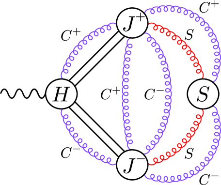
Figure 1: Leading regions for double-charmonium production in $e^{+}e^{-}$ annihilation. The wavy line represents the virtual photon.

There are two distinct topologies in the case of $B$-meson decays: one in which the $B$-meson and light-meson spectators participate in the hard interaction and another in which they do not. These two topologies are shown in Figs. 2(a) and 2(b), respectively. The topology of Fig. 2(a) is appropriate when the light-meson-antiquark momentum is outside the endpoint region, and the topology of Fig. 2(b) is appropriate when the light-meson-antiquark momentum is in the endpoint region.

In each topology in Fig. 2, there is a hard subdiagram that includes the lowest-order parton-level process, there is a soft subdiagram, and there is a jet subdiagram for each of the two collinear regions, which correspond to the light meson and the quarkonium. In the hard subdiagram, all propagator denominators are of order $m_{b}^{2}$ or $m_{b}\Lambda_{\rm QCD}$. The soft subdiagram includes gluons with soft momenta and loops involving quarks and ghosts with soft momenta. The soft subdiagram attaches to the jet subdiagrams and to the $B$-meson quark and antiquark quark lines through any number of soft gluon lines. The $J^{+}$ subdiagram contains the quarkonium quark and antiquark lines; the $J^{-}$ subdiagram contains the light-meson quark and antiquark lines; the $J^{l}$ subdiagram contains the $B$-meson spectator-quark line. In addition, the jet subdiagrams contain gluons and loops involving quarks, gluons, and ghosts with momenta in the $C^{\pm}$, or $C^{l}$ regions. Each jet subdiagram contains the active- and spectator-quark lines for a given meson or quarkonium as well as gluons and loops involving quarks, gluons, and ghosts with momenta collinear to the meson or quarkonium. A $J^{\pm}$ or $J^{l}$ subdiagram attaches to the hard subdiagram through the active- and spectator-quark lines in the topology of Fig. 2(a), through the active-quark lines in the topology of Fig. 2(b) and through any number of gluons. (We have not shown explicitly the attachments of the $J^{l}$ jet subdiagram that involve gluons with $C^{l}$ momenta.) As we have already mentioned, because gluons with $C^{i}$ momenta of arbitrarily low energy can contribute at leading power in $Q$, the $J^{\pm}$ subdiagram also attaches to the soft, $J^{\mp}$, and $J^{l}$ subdiagrams through any number of $C^{\pm}$ gluons, and the $J^{l}$ subdiagram also attaches to the soft and $J^{\pm}$ subdiagrams through any number of $C^{l}$ gluons Bodwin:2009cb .

In the case of the topology of Fig. 2(b), we show explicitly a gluon that is marked with an asterisk. This is the gluon that was mentioned in our discussion of the endpoint region in Sec. III.2.2. We choose the momentum routing so that it always carries the momentum of the $B$-meson antiquark and the (endpoint) momentum of the light-meson antiquark, both of which are of order $\Lambda_{\rm QCD}$. Therefore, we consider this gluon to be part of the soft subdiagram. However, we single it out because it must be present in our model in order for the light antiquarks (spectators) to be connected to the remainder of the diagram and because its momentum is fixed by the $B$-meson and light-meson antiquark momenta. Soft gluons and low-energy $C^{\pm}$ gluons can connect to the marked gluon, although we have not shown these connections explicitly. We show the marked gluon connecting to the hard subdiagram because its allowed connections to the jet subdiagrams or the $b$-quark line result in propagators with semihard virtualities, of order $m_{b}\Lambda_{\rm QCD}$, which are part of the hard subdiagram. As we have said, the topology of Fig. 2(b) applies to the endpoint region, in which the marked gluon has virtuality of order $\Lambda_{\rm QCD}^{2}$. Away from the endpoint region, the marked gluon itself has virtuality of order $m_{b}\Lambda_{\rm QCD}$ and can be incorporated into the hard subdiagram, resulting in the topology of Fig. 2(a).

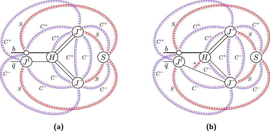
Figure 2: Leading regions for the $B$-meson-decay case. The collinear region $J^{+}$ corresponds to the charmonium and collinear region $J^{-}$ corresponds to the light meson.

III.4 Topologies of the Singular Regions

In the massless sector of QCD, there are singularities that are associated with soft and collinear divergences. (See, for example, Refs. Sterman:1978bi ; Sterman:1978bj ; Collins:1985ue ; Collins:1989gx .) In the present case, the masses of charm quarks and antiquarks cut off some of the collinear divergences. Some potential soft divergences are also cut off because they are associated with a gluon that attaches to a line that cannot go precisely to its mass shell because a quark mass cuts off a collinear divergence. Nevertheless, as we have mentioned, we wish to consider not only actual divergences, but also divergences that appear only in the limit $m_{c}/Q\to 0$ with $q_{i}$ fixed, because such divergences are associated with logarithmic enhancements. These divergences are associated with singularities in the domain of integrations. We call the infinitesimal neighborhoods of such singularities “singular regions.” In the remainder of the discussion of the factorization of the contributions of the singular regions, we assume that we have taken the limit $m_{c}/Q\to 0$ with $q_{i}$ fixed.

The topologies of the singular regions follow from the power-counting rules that are given in Sec. III.2. These topologies have been discussed in Ref. Bodwin:2009cb . Here, we recapitulate that discussion, describing the relationships of the topologies of the singular regions to the topologies of the leading regions in Figs. 1, 2(a), and 2(b).

The $C^{i}$ singular region is situated in the outermost part of the $J^{i}$ subdiagram. (Here, “out” means toward the external fermion lines.) We call this part of the $J^{i}$ subdiagram the $\tilde{J}^{i}$ subdiagram. (We denote the part of the $J^{i}$ subdiagram that excludes the $\tilde{J}^{i}$ subdiagram as the $J^{i}-\tilde{J}^{i}$ subdiagram.) The $S$ singular region is situated in the outermost part of the $S$ subdiagram. We call the $S$ singular part of the $S$ subdiagram the $\tilde{S}$ subdiagram. (We denote the part of the $S$ subdiagram that excludes the $\tilde{S}$ subdiagram as the $S-\tilde{S}$ subdiagram.) $S$ singular gluons connect the $\tilde{S}$ subdiagram only to the $\tilde{J}^{i}$ subdiagrams and to the external $b$-quark line. The gluon that is marked with an asterisk in the topology of Fig. 2(b) is not part of the $\tilde{S}$ subdiagram because its momentum components are fixed to be of order $\Lambda_{\rm QCD}$. That is, it is $S$ but not $S$ singular. The $\tilde{J}^{i}$ subdiagrams connect to the $J^{i}$, $S$, and $H$ subdiagrams via $C^{i}$ gluons. We denote by $\tilde{H}$ the union of all of the subdiagrams in our topology except for $\tilde{S}$, $\tilde{J}^{+}$, $\tilde{J}^{-}$, and $\tilde{J}^{l}$. We note that the connections of the $\tilde{J}^{\pm}$ subdiagrams to the $\tilde{S}$ subdiagram via $C^{i}$ gluons were not considered in the discussions in Refs. Collins:1985ue ; Collins:1989gx . Otherwise, the general structure of the topologies of the singular regions that we consider are the same as in Refs. Collins:1985ue ; Collins:1989gx , provided that we identify the hard subdiagram in those references with $\tilde{H}$.

III.5 Collinear approximation

We now describe the collinear approximations, which are useful in factoring the $C^{i}$ singular contributions. We follow the notation of Ref. Bodwin:2009cb .

Suppose that there is a gluon with momentum in the $C^{i}$ singular region that attaches to a line that is not in $\tilde{J}^{i}$. Then, we can apply a collinear approximation to that gluon Bodwin:1984hc ; Collins:1985ue ; Collins:1989gx without loss of accuracy. The $C^{i}$ approximation consists of replacing $g_{\mu\nu}$ in the gluon-propagator numerator as follows:

$$g_{\mu\nu}\,\,\longrightarrow\,\,\left\{\begin{array}[]{ll}\displaystyle\frac{k_{\mu}\tilde{n}_{1\nu}}{k\cdot\tilde{n}_{1}-i\varepsilon}&(C^{+}),\\[8.61108pt] \displaystyle\frac{k_{\mu}\tilde{n}_{2\nu}}{k\cdot\tilde{n}_{2}+i\varepsilon}&(C^{-}),\\[8.61108pt] \displaystyle\frac{k_{\mu}\tilde{n}_{l\nu}}{k\cdot\tilde{n}_{l}-i\varepsilon}&(C^{l}).\end{array}\right.$$ (34)

Here, the index $\mu$ corresponds to the attachment of the gluon to the line with momentum not in the $C^{i}$ singular region, and the index $\nu$ corresponds to the attachment of the gluon to the $J^{i}$ subdiagram. We always use the convention that $k$ flows out of a $C^{+}$ or $C^{l}$ line and into a $C^{-}$ line. There is a large amount of freedom in choosing the auxiliary vectors $\tilde{n}_{1}$, $\tilde{n}_{2}$ and $\tilde{n}_{l}$ in Eq. (34). We need only have $\tilde{n}_{1}\cdot p_{1q}>0$ (or $\tilde{n}_{1}\cdot p_{1\bar{q}}>0$), $\tilde{n}_{2}\cdot p_{2q}>0$ (or $\tilde{n}_{2}\cdot p_{2\bar{q}}>0$), and $\tilde{n}_{l}\cdot p_{l}>0$ in order to reproduce the amplitude in the collinear singular region. Our choice is to take $\tilde{n}_{1}$, $\tilde{n}_{2}$, and $\tilde{n}_{l}$ to be lightlike vectors in the minus, plus, and minus directions, respectively:

$$\tilde{n}_{1} = \bar{n}_{1}\equiv(1/\sqrt{2})(0,1,\bm{0}_{\perp}),$$ (35a)

$$\tilde{n}_{2} = \bar{n}_{2}\equiv(1/\sqrt{2})(1,0,\bm{0}_{\perp}),$$ (35b)

$$\tilde{n}_{l} = \bar{n}_{1}.$$ (35c)

In order for the $C^{i}$ approximation to be exact in the $C^{i}$ limit, $j\cdot k$ must be equal to $j^{\mp}k^{\pm}$, where $j$ is the current to which the $\mu$ index of the gluon with momentum $k$ attaches and $n_{i}$ is a unit lightlike vector in the $C^{i}$ direction. This requirement is met provided that the gluon does not attach with its $\mu$ index to a line that is also carrying momentum in the $C^{i}$ singular region. That is, the $C^{i}$ approximation holds in the collinear limit if $j$ is a current in any of the subdiagrams except for the $\tilde{J}^{i}$ subdiagram. We note that, in the $C^{i}$ approximation, the gluon’s polarization is longitudinal, i.e., proportional to the gluon’s momentum. This fact is essential to the application of graphical Ward identities to derive decoupling relations. We note also that the collinear approximation is exact, not only for the collinear singularity, but also for the associated collinear logarithmic enhancement.

III.6 Soft approximation

We now describe the soft approximation, which is useful in factoring the $S$ singular contributions. Again, we follow the notation of Ref. Bodwin:2009cb .

Suppose that there is a gluon with momentum $k$ in the $S$ singular region that attaches to a line carrying momentum $p$ that lies outside the $S$ singular region. Then we can apply the soft approximation to that gluon without loss of accuracy. The soft approximation Grammer:1973db ; Collins:1981uk consists of replacing $g_{\mu\nu}$ in the gluon-propagator numerator as follows:

$$g_{\mu\nu}\,\,\longrightarrow\,\,\frac{k_{\mu}p_{\nu}}{k\cdot p},$$ (36)

where the index $\mu$ corresponds to the attachment of the gluon to the line with momentum $p$.

Unlike the collinear approximation, the soft approximation depends on the momentum of the line to which the gluon attaches. However, it is convenient to apply the same soft approximation to all of the lines in the $\tilde{J}^{\pm}$ subdiagram. The lines in the $\tilde{J}^{\pm}$ subdiagram are collinear either to the momentum of the quark or the momentum of the antiquark in the jet. In the case of the light-quark jet, the quark and antiquark momenta are parallel, up to corrections of relative order $\Lambda_{\rm QCD}/Q$. In the case of the quarkonium jet(s), the quark and antiquark momenta $p_{iq}$ and $p_{i\bar{q}}$ are parallel up to corrections of relative order $m_{c}v/Q$. In both cases, we neglect the difference between the quark and antiquark momenta and define a “modified soft approximation” for each jet that corresponds to the soft approximation for the average of the quark and antiquark momenta. The leading errors that arise in applying the modified soft approximation to the light-meson, charmonium-1, and charmonium-2 jets are of relative order $\bm{q}_{k\perp}/p_{K}^{-}\sim\Lambda_{\rm QCD}/Q$, $\bm{q}_{1\perp}/P_{1}^{+}\sim m_{c}v/Q$, and $\bm{q}_{2\perp}/P_{2}^{-}\sim m_{c}v/Q$, respectively.

It is convenient, for purposes of discussing the decoupling relations in Sec. III.7, to choose lightlike vectors for the soft approximation that correspond to the average of the quark and antiquark momenta in the limits $\Lambda_{\rm QCD}/Q\to 0$ and $m_{c}/Q\to 0$. In making this choice, we introduce an error of relative order $\Lambda_{\rm QCD}^{2}/Q^{2}$ in the case of the light-meson jet and of relative order $m_{c}^{2}/Q^{2}$ in the case of the quarkonium jet(s). These errors are negligible in comparison with the errors that we make in neglecting the difference between the quark and antiquark momenta. Then, for both the light-meson and quarkonium jets we have the same soft approximations.

For the attachment of the gluon with momentum $k$ to any line with momentum in the $C^{+}$ ($C^{-}$) singular region, the (modified) soft approximation consists of the following replacements in the gluon-propagator numerator:

$$g_{\mu\nu} \longrightarrow \frac{k_{\mu}n_{1\nu}}{k\cdot n_{1}+i\varepsilon}(S^{+}),$$ (37a)

$$g_{\mu\nu} \longrightarrow \frac{k_{\mu}n_{2\nu}}{k\cdot n_{2}-i\varepsilon}(S^{-}),$$ (37b)

where $n_{1}$ is a lightlike vector that is proportional to $P_{1}$ and $n_{2}$ is a lightlike vector that is proportional to $P_{2}$ or $p_{K}$. We normalize $n_{1}$ and $n_{2}$ so that they are the parity inverses of the vectors $\bar{n}_{1}$ and $\bar{n}_{2}$ in Eq. (35), respectively:

$$n_{1} \equiv (1/\sqrt{2})(1,0,\bm{0}_{\perp}),$$ (38a)

$$n_{2} \equiv (1/\sqrt{2})(0,1,\bm{0}_{\perp}).$$ (38b)

The index $\mu$ contracts into the line carrying the momentum of type $C^{+}$ ($C^{-}$). As we have mentioned, the modified soft approximation in Eq. (37) accounts for the contributions in the $S$ singular region up to corrections of relative order $\Lambda_{\rm QCD}/Q$ in the case of the light-meson jet and up to corrections of relative order $m_{c}v/Q$ in the case of quarkonium jets. We note also that the soft approximation is valid at this accuracy not only for the soft singularity, but also for the associated soft logarithmic enhancement.

We do not apply soft approximations to the $B$ meson because the eikonal vectors that are associated with soft approximations for $J^{l}$ and the $b$-quark line are not approximately proportional to each other. That is, a common soft approximation cannot be applied to the $B$ meson. In consequence, the cancellations of the soft contributions that apply in the case of the quarkonia and the light meson (described in Sec. III.9.1) fail in the case of the $B$ meson.

III.7 Decoupling relations

Once we have implemented a collinear approximation or a soft approximation, the associated gluons are longitudinally polarized. This allows us to make use of decoupling relations to factor gluons with momenta in the soft or collinear singular regions from certain parts of the amplitude. The general graphical form of the decoupling relations for longitudinally polarized gluons is shown in Fig. 3.

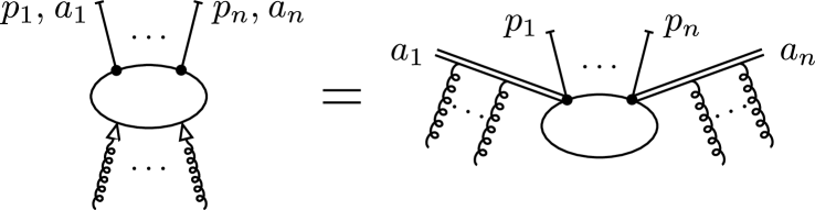
Figure 3: Graphical representation of the decoupling relations for collinear gluons and the decoupling relations for soft gluons. The applicability of these decoupling relations is described in the text. The relations show the decoupling of longitudinally polarized gluons, which are represented by curly lines. The longitudinally polarized gluon lines are to be attached in all possible ways to the Green’s function that is represented by an oval. The factors $k^{\mu}\bar{n}_{i}^{\nu}/(k\cdot\bar{n}_{i})$ [$k^{\mu}n_{i}^{\nu}/(k\cdot n_{i})$] that appear in the collinear (soft) approximations are represented by the arrows on the gluon lines. The external lines with hash marks are truncated. In addition, the subdiagram can include any number of untruncated on-shell external legs, provided that the polarizations of the on-shell gluons are orthogonal to their momentum. The $p_{i}$ are momenta, and the $a_{i}$ are color indices. The double lines are $C^{+}$, $C^{-}$, $S^{+}$, or $S^{-}$ eikonal lines, as is described in the text.

A decoupling relation of this form applies when any number of longitudinally polarized gluons attach to a subdiagram in all possible ways, provided that the gluon momenta are all proportional to each other.

If the external gluons all have momenta in one of the $C^{i}$ singular regions, then the gluon momenta are all proportional to each other, and a decoupling relation of the form in Fig. 3 holds, once the $C^{i}$ approximation has been implemented to render the gluon polarizations longitudinal. The subdiagram can have any number of truncated legs and any number of untruncated on-shell external legs (not shown in the figure), provided that the polarizations of the untruncated on-shell gluons are orthogonal to their momentum. The eikonal (double) lines in this decoupling relation have the Feynman rules in the $C^{+}$, $C^{-}$, or $C^{l}$ cases that a vertex is $\mp igT_{a}\bar{n}_{1\mu}$, $\pm igT_{a}\bar{n}_{2\mu}$, or $igT_{a}\bar{n}_{l\mu}$ and a propagator is $i/(k\cdot\bar{n}_{1}-i\varepsilon)$, $i/(k\cdot\bar{n}_{2}+i\varepsilon)$, $i/(k\cdot\bar{n}_{l}-i\varepsilon)$, respectively, where the upper (lower) sign in the vertex is for eikonal lines that attach to quark (antiquark) lines. Here, $T_{a}$ is an $SU(3)$ color matrix in the fundamental representation. (Our convention is that a QCD gluon-quark vertex is $igT_{a}\gamma_{\mu}$.) We call these eikonal lines “$C^{i}$ eikonal lines.” The Feynman rules for the eikonal lines in these decoupling relations are summarized in the first, second, and third lines of Table 2.

If the external gluons all have momenta in the $S$ singular region, then the decoupling requirement that the gluon momenta be proportional to each other is not necessarily satisfied. However, if the subdiagram into which the $S$ singular gluons enter is a $\tilde{J}^{+}$ ($\tilde{J}^{-}$) subdiagram, then a soft momentum $k$ entering that subdiagram contracts only into currents proportional to $n_{1}$ ($n_{2}$), up to corrections of relative order $\bm{q}_{k2}/p_{K}^{-}\sim\Lambda_{\rm QCD}/Q$ for a light-meson jet and relative order $\bm{q}_{1\perp}/P_{1}^{+}\sim\bm{q}_{2\perp}/P_{2}^{-}\sim m_{c}v/Q$ for a charmonium jet. Consequently, at these levels of accuracy, we can make the replacement

$$k\to\tilde{k}_{1}=\bar{n}_{1}\frac{n_{1}\cdot k}{n_{1}\cdot\bar{n}_{1}}$$ (39a)

in the $$\tilde{J}^{+}$$ subdiagram and associated soft approximation and the replacement

$$k\to\tilde{k}_{2}=\bar{n}_{2}\frac{n_{2}\cdot k}{n_{2}\cdot\bar{n}_{2}}$$ (39b)

in the $\tilde{J}^{-}$ subdiagram and associated soft approximation Collins:1985ue ; Collins:1989gx . Since

$$n_{1}\cdot\tilde{k}_{1} = n_{1}\cdot k,$$ (40a)

$$n_{2}\cdot\tilde{k}_{2} = n_{2}\cdot k,$$ (40b)

these replacements do not change the amplitude, up to corrections of relative order $m_{c}/Q$ and $\Lambda_{\rm QCD}/Q$. In subsequent discussions, we consider these replacements to be part of the modified soft approximation. After these replacements have been made, the gluon momenta entering the $\tilde{J}^{+}$ ($\tilde{J}^{-}$) subdiagram are all proportional to each other, and a decoupling relation of the form in Fig. 3 holds. In these decoupling relations, the eikonal lines have the Feynman rules that a vertex is $\pm igT_{a}n_{1\mu}$ ($\mp igT_{a}n_{2\mu}$) and a propagator is $i/(k\cdot n_{1}+i\varepsilon)$ [$i/(k\cdot n_{2}-i\varepsilon)$] when the subdiagram is $C^{+}$ ($C^{-}$). These rules follow from Eq. (40). We call these eikonal lines $S^{+}$ and $S^{-}$ eikonal lines, respectively. The Feynman rules for the eikonal lines in the soft decoupling relations are summarized in the fourth and fifth lines of Table 2, respectively.

Type	Vertex	Propagator
$C^{+}$	$\mp igT_{a}\bar{n}_{1\mu}$	$\displaystyle\frac{i}{k\cdot\bar{n}_{1}-i\varepsilon}$
$C^{-}$	$\pm igT_{a}\bar{n}_{2\mu}$	$\displaystyle\frac{i}{k\cdot\bar{n}_{2}+i\varepsilon}$
$C^{l}$	$igT_{a}\bar{n}_{l\mu}$	$\displaystyle\frac{i}{k\cdot\bar{n}_{l}-i\varepsilon}$
$S^{+}$	$\pm igT_{a}n_{1\mu}$	$\displaystyle\frac{i}{k\cdot{n}_{1}+i\varepsilon}$
$S^{-}$	$\mp igT_{a}n_{2\mu}$	$\displaystyle\frac{i}{k\cdot{n}_{2}-i\varepsilon}$

Table 2: Feynman rules for the collinear ($C^{\pm}$ and $C^{l}$) and soft ($S^{\pm}$) eikonal lines. The upper (lower) sign is for the eikonal line that attaches to a quark (antiquark) line.

III.8 Factorization of the singular regions

Now we summarize the factorization of the singular regions. We refer the reader to Ref. Bodwin:2009cb for detailed arguments.

In analyzing the singular regions, we wish to identify the momentum configurations that yield singular contributions. We can do so by making use of the power-counting rules that we have outlined in Sec. III.2 and invoking the following specific interpretations of those rules: the symbol $\sim$ and the phrase “of the same order” mean that quantities differ by a finite factor, while the phrases “much less than” and “much greater than” mean that quantities differ by an infinite factor. It follows that, for gluons in the singular regions, our convention that an allowed attachment of a gluon cannot change the essential nature of the momentum of the line to which it attaches has the following meaning: The attaching gluon cannot have an energy that is greater by an infinite factor than the energy of the line to which it attaches.

The rules in Sec. III.2 lead to complicated relationships between the allowed momenta of gluons in a given diagrammatic topology. However, there is a general principle, which we have already mentioned, that allows us to organize the discussion: The attachments of gluons to a given line must be ordered so that a given attachment produces a virtuality along the line that is of order or greater than the virtualities that are produced by the attachments that lie to the outside of it. In particular, the virtuality that a $C^{i}$, or $S$ singular gluon produces on a $C^{j}$ line with $j\neq i$ or an $S$ line is of order the energy of gluon times the energy of the line to which it attaches.

Our goal is to factor $C^{\pm}$ contributions from all subdiagrams except $\tilde{J}^{\pm}$, to factor all $C^{l}$ singular contributions from all subdiagrams except $\tilde{J}^{l}$ and the external $b$-quark line and to factor all $S$ singular contributions from the $\tilde{J}^{\pm}$ subdiagrams. We will show that the factored soft contributions that are associated with the external-quark and external-antiquark lines in $\tilde{J}^{\pm}$ ultimately cancel.

Note that we do not factor $S$ singular contributions from $\tilde{J}^{l}$ or from the external $b$-quark line. Nor do we factor $C^{l}$ singular contributions from the external $b$-quark line in the $B$-meson subdiagram. In principle, we could carry out such factorizations. However, because the soft approximations are different for the $b$ quark and the light antiquark in the $B$ meson, we do not expect the factored soft contributions that are associated with the $b$-quark and light-antiquark lines to cancel. Furthermore, it will prove convenient, for purposes of expressing our results in terms of a $B$-meson light-cone distribution, not to factor the $C^{l}$ singular contributions from the $b$-quark line in the $B$-meson subdiagram.

In the singular limits $\epsilon_{S}\to 0$, $\eta^{i}\to 0$, $\epsilon^{i}\to 0$, an infinite hierarchy of energy scales emerges. The energy scales of the various levels in the hierarchy are separated by infinite factors. We characterize each level in the hierarchy by the energy scale of the $S$ singular gluons in that level. We call this scale the nominal energy scale of that level. Collinear singular gluons in a level may have energies that are of the nominal energy scale or energies that are infinitely larger than the nominal scale, but still infinitesimal in comparison with the nominal energy scale of the next higher level. We call the latter gluons “large-scale collinear singular gluons.” We carry out the factorization iteratively, starting with the level with the largest nominal energy scale. As we shall see, this ordering of the factorization procedure is convenient because it allows us to apply the decoupling relations rather straightforwardly to decouple gluons whose connections lie toward the inside of the Feynman diagrams before we decouple gluons whose connections lie to the outside of the Feynman diagrams.

We will illustrate the factorization of the large-scale collinear gluons and the nominal-scale soft and collinear gluons for the case of double-charmonium production in $e^{+}e^{-}$ annihilation by referring to the diagram that is shown in Fig. 4. In this diagram, we have suppressed gluons with energies that are much less than the nominal scale. These gluons have connections that lie to the outside of the connections of the gluons that are shown explicitly. In the diagram in Fig. 4, each gluon represents any finite number of gluons, including zero gluons. For clarity, we have suppressed the antiquark lines in each meson and we have shown explicitly only the connections of the gluons to the quark line in each meson and only a particular ordering of those connections. However, we take the diagram in Fig. 4 to represent a sum of many diagrams, which include all of the connections that we specify in the arguments below of the singular gluons to the quark and antiquark in each meson, to other singular gluons, and to the $\tilde{H}$ subdiagram.

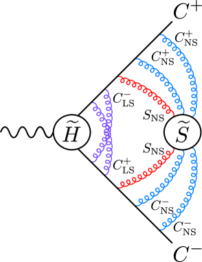
Figure 4: Diagram to illustrate the factorization of large-scale collinear gluons and nominal-scale soft and collinear gluons for the case of double-charmonium production in $e^{+}e^{-}$ annihilation. $C^{i}_{\textrm{LS}}$ denotes a large-scale $C^{i}$ singular gluon, $C^{i}_{\textrm{NS}}$ denotes a nominal-scale $C^{i}$ singular gluon, and $S_{\textrm{NS}}$ denotes a nominal-scale $S$ singular gluon.

III.8.1 Factorization of the large-scale $C^{i}$ singular gluons

First, we factor the large-scale $C^{i}$ singular gluons. In the first step of the iteration, these include gluons with finite energies, as well as infinitesimal energies. In subsequent steps, only gluons with infinitesimal energies are involved. There is a hierarchy in the energy scales of the large-scale $C^{i}$ singular gluons. We factor these gluons iteratively, beginning with the largest energy scale.

We apply the $C^{i}$ approximations and the $C^{i}$ decoupling relations. In applying the $C^{\pm}$ decoupling relations, we include the attachments that are allowed by our conventions to all subdiagrams outside of $\tilde{J}^{\pm}$, and, in applying the $C^{l}$ decoupling relations, we include the attachments that are allowed by our conventions to all subdiagrams outside of $\tilde{J}^{l}$ and the external $b$-quark line. We also include, formally some attachments that may yield vanishing contributions in the singular limits. These are attachments to $\tilde{H}$ and attachments that lie to the inside of the allowed attachments to $\tilde{J^{j}}$ for $j\neq i$. We include in this class attachments to the interior of $C^{j}$ eikonal lines. (“Interior” means to the inside of attachments of $C^{j}$ gluons.)

The outermost allowed attachment of $C^{i}$ gluon to a $C^{j}$ singular line in $\tilde{J}^{j}$ ($i\neq j$) generally lies to the inside of attachments of additional gluons that have infinitesimally smaller energy scales. While the propagator immediately to the outside of the outermost allowed attachment of $C^{i}$ gluon is not precisely on the mass shell, it is on the mass shell, up to relatively infinitesimal corrections. Furthermore, if it is a gluon propagator, then its polarization is orthogonal to its momentum, up to relatively infinitesimal corrections. Therefore, when we apply the $C^{+}$ decoupling relation, no eikonal-line contribution appears at this point.

The result of the application of the $C^{i}$ decoupling relations to the large-scale $C^{i}$ singular gluons with the largest energies is that the connections of these gluons to subdiagrams other than $\tilde{J}^{i}$ and the $b$-quark line are replaced with connections to $C^{i}$ eikonal lines. The $C^{\pm}$ eikonal lines attach to the $C^{\pm}$ external-fermion lines just to the outside of $\tilde{H}$. (Here, and in subsequent discussions, “external-fermion lines” denote the fermion lines that originate in the external quarks and antiquarks that are associated with the mesons in our model.) The $C^{l}$ eikonal lines attach to the external $b$-quark line and the external light-quark line from the $B$ meson just to the outside of $\tilde{H}$.

We can iterate this procedure for large-scale $C^{i}$ singular gluons with successively lower energy scales. After each iteration, there is a new $C^{i}$ eikonal line that attaches to each $C^{i}$ external-fermion line just to the inside of the $C^{i}$ eikonal line from the previous iteration. It is easy to see that, for each external-fermion line, the new eikonal line can be combined with the eikonal line from the previous iteration to form a single eikonal line, on which the $C^{i}$ singular gluons with lower energy scale attach to the outside of the $C^{i}$ singular gluons with higher energy scales. Other orderings of the attachments yield vanishing contributions. We continue iteratively in this fashion until we have factored all of the large-scale $C^{i}$ gluons. After this decoupling step, the sum of diagrams represented by Fig. 4 becomes a sum of diagrams represented by Fig. 5.

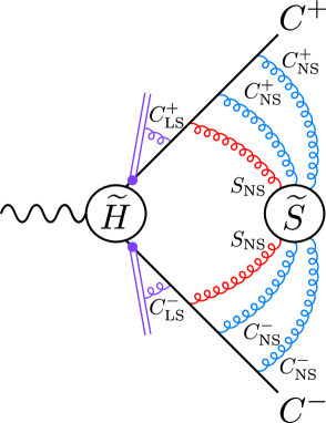
Figure 5: Diagram representing the sum of diagrams that occurs after one applies the decoupling of the large-scale collinear gluons that is described in Sec. III.8.1.

III.8.2 Initial factorization of the nominal-scale $C^{i}$ gluons

Next, we factor the nominal-scale $C^{i}$ singular gluons. In addition to the attachments enumerated in the case of the large-scale $C^{i}$ gluons, we include attachments to the nominal-scale $S$ gluons. Then, the application of the $C^{\pm}$ decoupling relations leads to $C^{\pm}$ eikonal lines that attach to the following locations: to the $C^{\pm}$ external-fermion lines just to the inside of the large-scale $C^{\pm}$ eikonal lines from the previous step; to the nominal-scale $S$ singular gluon lines just to the inside of the connections of those lines to the $C^{\pm}$ external-fermion lines. After this decoupling step, the sum of diagrams represented by Fig. 5 becomes a sum of diagrams represented by Fig. 6. Application of the $C^{l}$ decoupling relation leads to $C^{l}$ eikonal lines that attach to the following locations: to the external-fermion lines from the $B$ meson just to the inside of the large-scale $C^{l}$ eikonal lines from the previous step; to the nominal-scale $S$ singular gluon lines just to the inside of the connections of those lines to the external-fermion lines from the $B$ meson. The $C^{l}$ eikonal line that attaches to a given external-fermion line from the $B$ meson can be combined with the large-scale $C^{l}$ eikonal line from the previous step to form a single $C^{l}$ eikonal line.

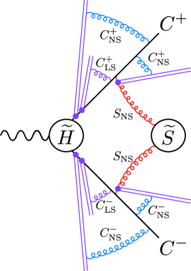
Figure 6: Diagram representing the sum of diagrams that occurs after one applies the initial decoupling of the nominal-scale collinear gluons that is described in Sec. III.8.2.

III.8.3 Factorization of the nominal-scale $S$ gluons

We now wish to apply the soft decoupling relations to factor the nominal-scale soft gluons. In order to do this, we implement the $S^{\pm}$ approximations for the allowed attachments of the soft gluons to $\tilde{J}^{\pm}$. (Recall that we do not apply the soft approximations or the soft decoupling relations to the attachments of the soft gluons to the external $b$-quark line or to $\tilde{J}^{l}$.) On the connections to the $\tilde{J}^{\pm}$ subdiagrams, we modify the soft approximation in the following way: We combine the momentum of the nominal-scale soft gluon with the total momentum of the attached nominal-scale $C^{\pm}$ eikonal line from the previous step. Then, when we implement the $S^{\pm}$ decoupling relations, the nominal-scale $C^{\pm}$ eikonal lines are carried along with the nominal-scale soft-gluon attachments. We apply the $S^{\pm}$ decoupling relations to the allowed attachments of the soft gluons to $\tilde{J}^{\pm}$. We also include vanishing connections of the nominal-scale soft gluons to the interior of the large-scale $C^{\pm}$ eikonal lines Collins:1985ue . The propagator that lies to the outside of the outermost allowed connection of a nominal-scale soft gluon to a line in $\tilde{J}^{\pm}$ is on shell, up to relative corrections of infinitesimal size. Furthermore, if it is a gluon propagator, its polarization is transverse to its momentum, up to relative corrections of infinitesimal size. Therefore, when we apply the $S^{\pm}$ decoupling relations, no $S^{\pm}$ eikonal lines appear at those points.

The result of applying the $S^{\pm}$ decoupling relations is that soft gluons attach to $S^{\pm}$ eikonal lines, to the external $b$-quark line and to $\tilde{J}^{l}$. The $S^{\pm}$ eikonal lines attach to the $C^{\pm}$ external-fermion lines just to the outside of the nominal-scale $C^{\pm}$ eikonal lines and just to the inside of the large-scale $C^{\pm}$ eikonal lines. Associated with each connection of a nominal-scale soft gluon to an $S^{\pm}$ eikonal line is a $C^{\pm}$ eikonal line. Associated with each connection of a nominal-scale soft gluon to the external $b$-quark line or to $\tilde{J}^{l}$ is a $C^{l}$ eikonal line. Our sample diagram is now given by Fig. 7.

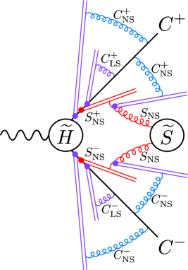
Figure 7: Diagram representing the sum of diagrams that occurs after one applies the decoupling of the nominal-scale soft gluons that is described in Sec. III.8.3.

III.8.4 Further factorization of the nominal-scale $C^{\pm}$ gluons

We next factor the nominal-scale $C^{\pm}$ gluons from the $S^{\pm}$ eikonal lines. In order do this, we include formally the vanishing contributions that arise when one connects the nominal-scale $C^{\pm}$ gluons to all points on the $S^{\pm}$ eikonal lines that lie to the inside of the outermost connection of the nominal-scale soft gluons. We also make use of the following facts: a nominal-scale $C^{\pm}$ eikonal line that attaches to one of the $C^{\pm}$ external-fermion lines is identical to the eikonal line that one would obtain by applying the $C^{\pm}$ decoupling relation to the attachments of the nominal-scale $C^{\pm}$ gluons to an on-shell fermion line (that does not have exactly $C^{\pm}$ momentum); a nominal-scale $C^{\pm}$ eikonal line that attaches to a nominal-scale gluon is identical to the eikonal line that one would obtain by applying the $C^{\pm}$ decoupling relation to the attachments of nominal-scale $C^{\pm}$ gluons to an on-shell nominal-scale soft-gluon line. Then, applying the $C^{\pm}$ decoupling relation, we find that the nominal-scale $C^{\pm}$ gluons attach to $C^{\pm}$ eikonal lines that attach to the external-fermion lines just to the inside of the large-scale $C^{\pm}$ eikonal lines. This situation is represented by the diagram that is shown in Fig. 8.

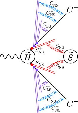
Figure 8: Diagram representing the sum of diagrams that occurs after one applies the further decoupling of the nominal-scale collinear gluons that is described in Sec. III.8.4.

The nominal-scale $C^{\pm}$ eikonal lines can then be combined with the large-scale $C^{\pm}$ eikonal lines. After performing those steps we arrive at the final factorized form for our sample diagram, which is given in Fig. 9.

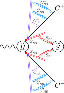
Figure 9: Diagram representing the sum of diagrams that occurs after one completely decouples the large-scale collinear gluons and the nominal-scale soft and collinear gluons.

III.8.5 Completion of the factorization

Now we can iterate the procedure that we have given in Secs. III.8.1–III.8.4, taking the nominal scale to be the next smaller soft-gluon scale. In these subsequent iterations, we include the connections of soft and collinear gluons that have already been described. In addition, we include formally, in the steps of Secs. III.8.1 and III.8.2, the vanishing contributions from the connections of the large-scale and nominal-scale $C^{i}$ gluons to the soft gluons of higher energies and to the $S^{\pm}$ eikonal lines that are associated with those soft gluons.

Proceeding iteratively through all of the soft-gluon scales, we produce new nominal-scale $S^{\pm}$ eikonal lines at each step that connect to the external $C^{\pm}$ fermion lines just to the outside of the existing $S^{\pm}$ eikonal lines. Each gluon that attaches to a nominal-scale $S^{\pm}$ eikonal line has attached to it a $C^{\pm}$ eikonal line. In addition, there are nominal-scale $C^{\pm}$ eikonal lines from the steps of Sec. III.8.2 that attach to the $C^{\pm}$ external-fermion lines just to the inside of the nominal-scale $S^{\pm}$ eikonal lines. After the further factorization of the nominal-scale $C^{\pm}$ gluons that is described in Sec. III.8.4, both of the $S^{\pm}$ eikonal lines that attach to a given external-fermion line can be combined into a single $S^{\pm}$ eikonal line.

At each step in the iteration, new $C^{l}$ eikonal lines appear that attach to the external-fermion lines from the $B$ meson just to the inside of the $C^{l}$ eikonal lines from the previous step. For each external-fermion line, the new $C^{l}$ eikonal line can be combined with the $C^{l}$ eikonal line from the previous step to form a single eikonal line. Similarly, at each step in the iteration, new $C^{l}$ eikonal lines appear that attach to the nominal-scale $S$ singular gluon lines that attach to the external fermion lines from the $B$ meson. These new $C^{l}$ eikonal lines attach just to the inside of the $C^{l}$ eikonal lines from the previous iteration. Again, for each external-fermion line, the new $C^{l}$ eikonal line can be combined with the previous $C^{l}$ eikonal line to form a single $C^{l}$ eikonal line.

Following this procedure, we arrive at the factorized form for the singular contributions. The $\tilde{S}$ subdiagram now connects only to $S^{\pm}$ eikonal lines, to the external $b$-quark line, and to $\tilde{J}^{l}$. The $S^{\pm}$ eikonal lines attach to the $C^{\pm}$ external-fermion lines just outside of $\tilde{H}$. All of the $C^{\pm}$ singular contributions are contained in the $J^{\pm}$ subdiagram and the associated $C^{\pm}$ eikonal lines, which attach to the $C^{\pm}$ external-fermion lines just outside of the $S^{\pm}$ eikonal lines. All of the $C^{l}$ contributions are contained in the $\tilde{J}^{l}$ subdiagram and associated $C^{l}$ eikonal lines. These $C^{l}$ eikonal lines attach to the external-fermion lines from the $B$ meson just to the outside of the $\tilde{H}$ subdiagram and to $S$ singular gluon lines just to the inside of the connections of those lines to the $b$-quark line and to $\tilde{J}^{l}$. This factorization is illustrated, for the case of $e^{+}e^{-}$ annihilation, in Fig. 10.

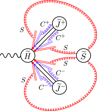
Figure 10: Illustration of the factorization for the case of $e^{+}e^{-}$ annihilation. After the use of the decoupling relations, gluons with momenta in the $S$ singular region attach to $S^{\pm}$ eikonal lines and gluons with momenta in the $C^{\pm}$ singular regions attach to $C^{\pm}$ eikonal lines.

III.9 Forms of the $\tilde{S}$ and $\tilde{J^{\pm}}$ functions and cancellations of eikonal lines

III.9.1 Cancellations of the soft eikonal lines

At this point, in the case of $e^{+}e^{-}$ annihilation into two quarkonia, the $\tilde{S}$ subdiagram and associated soft eikonal lines, which we call $\bar{S}$, take the form of the vacuum-expectation value of a time-ordered product of four eikonal lines:

$$\bar{S}(x_{1q},x_{1\bar{q}},x_{2q},x_{2\bar{q}})=\langle 0|T\{[x_{1\bar{q}},\infty^{+}][\infty^{+},x_{1q}]\otimes[x_{2\bar{q}},\infty^{-}][\infty^{-},x_{2q}]\}|0\rangle_{S},$$ (41)

where $x_{iq}$ and $x_{i\bar{q}}$ are the points at which the eikonal lines attach to the quark and antiquark external lines from meson 1 and meson 2, respectively. $[y,x]$ is the eikonal line that is defined in Eq. (6), $\infty^{+}=(\infty,0,\bm{0}_{\perp})$, and $\infty^{-}=(0,\infty,\bm{0}_{\perp})$. The symbol $\otimes$ indicates a direct product of the color factors that are associated with the soft-gluon attachments to meson 1 and the soft-gluon attachments to meson 2. The $S$ subscript on the matrix element indicates that only the contributions from the $S$ singular region are kept.

In the case of $B$-meson decays, the $\tilde{S}$ subdiagram is still connected to the $B$ meson and takes the form

$$\bar{S}_{B}(x_{1q},x_{1\bar{q}},x_{2q},x_{2\bar{q}})=\left<0|T\{[x_{1\bar{q}},\infty^{+}][\infty^{+},x_{1q}]\otimes[x_{2\bar{q}},\infty^{-}][\infty^{-},x_{2q}]\}\bar{\Psi}_{l}\Gamma_{Bm}\Psi_{b}|B\right>_{S}.$$ (42)

Here, we have suppressed the $C^{l}$ eikonal lines that are associated with the $B$ meson. No soft gluons attach to those lines.

Because the $\tilde{H}$ subdiagram is insensitive to a momentum in the $S$ singular region that flows through it, one can ignore the difference between $x_{1q}$ and $x_{1\bar{q}}$ and the difference between $x_{2q}$ and $x_{2\bar{q}}$. Therefore, in consequence of the fact that the external mesons are color singlets, the $S^{+}$ quark and antiquark eikonal lines cancel, and the $S^{-}$ quark and antiquark eikonal lines cancel. In the case of $e^{+}e^{-}$ annihilation into two quarkonia, this cancellation implies that the $\tilde{S}$ subdiagram is completely disconnected, and, therefore, can be ignored. In the case of $B$-meson decays, the remaining $\tilde{S}$ subdiagram now connects only to the external $b$-quark line and to $\tilde{J}^{l}$.

III.9.2 Rearrangement of the $B$-meson singular contributions

As we have noted, there are $C^{l}$ eikonal lines associated with the $B$ meson. These $C^{l}$ eikonal lines attach to the external-fermion lines from the $B$ meson just to the outside of the $\tilde{H}$ subdiagram and to $S$ singular gluon lines just to the inside of the connections of those lines to the external $b$-quark line and to $\tilde{J}^{l}$. We can now remove the latter class of eikonal lines as follows. We note that, because the $\tilde{S}$ subdiagram now connects only to the external $b$-quark line and to $\tilde{J}^{l}$, the $C^{l}$ eikonal lines that attach to the $S$ singular gluons are precisely the $C^{l}$ eikonal lines that would appear if one were to factor connections of $C^{l}$ singular gluons from $\tilde{S}$. (One can carry out the factorization iteratively, level-by-level, factoring the nominal-scale $C^{l}$ gluons from the nominal-scale $S$ singular gluons.) Therefore, we restore the connections of the $C^{l}$ singular gluons to $\tilde{S}$ and drop the $C^{l}$ eikonal lines that attach to $S$ singular gluons.

III.9.3 Forms of the meson distributions

We make a Fierz rearrangement to decouple the color structures of the $\tilde{J}^{\pm}$ subdiagrams, the $b$-quark and $\tilde{J}^{l}$ subdiagram, and their associated collinear eikonal lines. Then, these subdiagrams and their eikonal lines are given by the following matrix elements:

$$\bar{J}_{\alpha\beta}^{+}(\bar{q}_{1})=\int_{-\infty}^{+\infty}d^{4}(2x)\exp[-2i\bar{q}_{1}\cdot x]\langle H_{1}(P_{1})|\bar{\Psi}_{\alpha}(x)T\{[x,\infty^{-}][\infty^{-},-x]\}\Psi_{\beta}(-x)|0\rangle_{C^{+}}$$ (43)

for the $C^{+}$ quarkonium,

$$\bar{J}_{\alpha\beta}^{-}(\bar{q}_{2})=\int_{-\infty}^{+\infty}d^{4}(2x)\exp[-2i\bar{q}_{2}\cdot x]\langle H_{2}(P_{2})|\bar{\Psi}_{\alpha}(x)T\{[x,\infty^{+}][\infty^{+},-x]\}\Psi_{\beta}(-x)|0\rangle_{C^{-}}$$ (44)

for the $C^{-}$ quarkonium,

$$\bar{J}_{K\alpha\beta}(\bar{r}_{k})=\int_{-\infty}^{+\infty}d^{4}(2x)\exp[-2i\bar{r}_{k}\cdot x]\langle K(p_{K})|\bar{\Psi}_{\alpha}(x)T\{[x,\infty^{+}][\infty^{+},-x]\}\Psi_{\beta}(-x)|0\rangle_{C^{-}}$$ (45)

for the light meson, and

$$\bar{J}_{B\alpha\beta}(\bar{p}_{l})=\int_{-\infty}^{+\infty}d^{4}x\exp[i\bar{p}_{l}\cdot x]\langle 0|\bar{\Psi}_{l\beta}(x)T\{[x,\infty^{-}][\infty^{-},0]\}\Psi_{b\alpha}(0)|B(p_{B})\rangle_{S,C^{l}}.$$ (46)

for the $B$ meson. In Eqs. (43)–(46), $\alpha$ and $\beta$ are Dirac indices. It is understood that the fields $\Psi$ and $\bar{\Psi}$ in each matrix element are in a color-singlet state. In these distributions, the arguments $\bar{q}_{1}$, $\bar{q}_{2}$, and $\bar{r}_{k}$ are each half the difference between the quark momentum and the antiquark momentum at the points at which they enter $\tilde{H}$, and the argument $\bar{q}_{l}$ is the antiquark momentum at the point at which it enters $\tilde{H}$. We have suppressed the dependences on the total meson momenta $P_{1}$, $P_{2}$, $p_{K}$, and $p_{B}$ in the arguments on the left sides of Eqs. (43)–(46). The subscripts $S$, $C^{+}$, $C^{-}$ and $C^{l}$ on the matrix elements indicate that we are retaining only the $S$, $C^{+}$, $C^{-}$, and $C^{l}$ singular contributions.

III.9.4 Light-cone distributions and cancellations of the collinear eikonal lines

Away from the endpoint region, we can simplify the factorized expression further.

In $\tilde{H}$, away from the endpoint region, we can approximate the momenta of the quark and antiquark in the light meson by their minus components. The leading relative errors in this approximation are of order $q_{k}/p_{K}\sim\Lambda_{\rm QCD}/Q$. Then, integrating $\bar{J}_{K}$ over $\bar{r}_{k}^{+}$ and $\bar{\bm{r}}_{k\perp}$, we obtain

$$\bar{J}_{K\alpha\beta}(y) \equiv \frac{p_{K}^{-}}{2\pi}\int_{-\infty}^{+\infty}\frac{d\bar{r}_{k}^{+}\,d^{2}\bar{\bm{r}}_{k\perp}}{(2\pi)^{3}}\,\bar{J}_{K\alpha\beta}(\bar{r}_{k})$$ (47)

$$= \frac{p_{K}^{-}}{\pi}\int_{-\infty}^{+\infty}dx^{+}\exp[-i(2y-1)p_{K}^{-}x^{+}]$$

$$\qquad\times\,\langle K(p_{K})|\bar{\Psi}_{\alpha}(x^{+})T\{[x^{+},\infty^{+}][\infty^{+},-x^{+}]\}\Psi_{\beta}(-x^{+})|0\rangle_{C^{-}}.$$

The quantity $\tilde{H}$ has been analyzed in the context of soft-collinear effective theory (SCET) for the case of $B$-meson decays into a lepton pair plus a photon Bosch:2003fc and for the contribution to $B$-meson decays into two light mesons that arises away from the endpoint region Beneke:2003pa . The conclusion of these analyses is that $\tilde{H}$ is given, to leading order in $\Lambda_{\rm QCD}/Q$, by a matrix element of a SCET operator that depends only on the plus component of the momentum of the light antiquark in the $B$ meson. Furthermore, the SCET operator has a Dirac-matrix structure such that only the $B$-meson light-cone distribution $\Phi_{B1}$ contributes. We assume that a similar SCET analysis holds in the case of $B$ meson decays to a quarkonium plus a light meson away from the endpoint region. Then, integrating $\bar{J}_{B}$ over $p_{l}^{-}$ and $\bm{p}_{l\perp}$, we obtain

$$\bar{J}_{B\alpha\beta}(\xi) \equiv \frac{p_{B}^{+}}{2\pi}\int_{-\infty}^{+\infty}\frac{dp_{l}^{-}\,d^{2}\bar{\bm{p}}_{l\perp}}{(2\pi)^{3}}\,\bar{J}_{B\alpha\beta}(p_{l})$$ (48)

$$= \frac{p_{B}^{+}}{2\pi}\int_{-\infty}^{+\infty}dx^{-}\exp[i\xi p_{B}^{+}x^{-}]$$

$$\qquad\times\,\langle 0|\bar{\Psi}_{l\beta}(x^{-})T\{[x^{-},\infty^{-}][\infty^{-},0]\}\Psi_{b\alpha}(0)|B(p_{B})\rangle_{C^{+}},$$

where $\xi=p_{l}^{+}/Q$.

We do not approximate the momenta of the heavy-quark and heavy antiquark in the quarkonia by their dominant momentum components because, in so doing, we would introduce errors of relative order $m_{c}v/Q$ for each quarkonium. As we will explain in Sec. III.11, such an error would be larger than the errors that arise from the approximations that we have used to derive the factorization result.

Now, we can see that there is a partial cancellation of the $C^{-}$ quark and antiquark eikonal lines in Eq. (47) and a partial cancellation of the $C^{l}$ quark and antiquark eikonal lines in Eq. (48). The cancellations would be complete, were it not for the fact that the $\tilde{H}$ subdiagram is sensitive the routing of collinear momenta through it. This sensitivity corresponds to the separation in space-time of the points $x^{+}$ and $-x^{+}$ in Eq. (47) and the points $x^{-}$ and $0$ in Eq. (48). The quark and antiquark eikonal lines in Eqs. (47) and (48) cancel where they overlap, leaving an eikonal line that runs directly between the quark and the antiquark:

$$\bar{J}_{K\alpha\beta}(y) = \frac{p_{K}^{-}}{\pi}\int_{-\infty}^{+\infty}dx^{+}\exp[-i(2y-1)p_{K}^{-}x^{+}]\langle K(p_{K})|\bar{\Psi}_{\alpha}(x^{+})P[x^{+},-x^{+}]\Psi_{\beta}(-x^{+})|0\rangle_{C^{-}}$$ (49a)

$$\equiv \sum_{j}\Phi_{Kj}(y)\left[\Gamma_{Kj}\right]_{\alpha\beta},$$

$$\bar{J}_{B\alpha\beta}(\xi) = \frac{p_{B}^{+}}{2\pi}\int_{-\infty}^{+\infty}dx^{-}\exp[i\xi p_{B}^{+}x^{-}]\langle 0|\bar{\Psi}_{l\beta}(x^{-})P[x^{-},0]\Psi_{b\alpha}(0)|B(p_{B})\rangle_{C^{+}}$$ (49b)

$$\equiv \sum_{m}\Phi_{Bm}(\xi)\left[\Gamma_{Bm}\right]_{\alpha\beta},$$

where we have written the time-ordered product of the exponentiated line integral as a path-ordered product. The expressions in Eqs. (49) have the form of the conventional light-meson and $B$-meson light-cone distributions, but, at this stage, they contain only the singular contributions to those light-cone distributions. Since the integrations over $y$ and $\xi$ have a finite range of support in $\tilde{H}$, the typical separation of the points $x^{+}$ and $-x^{+}$ in Eq. (49a) and the points $x^{-}$ and $0$ in Eq. (49b) is of order $1/Q$.

III.10 Factorized form

III.10.1 Factorization of the logarithmic enhancements

At this point, we have established that the contributions from the soft singular region decouple completely from the $\tilde{J}^{\pm}$ subdiagrams (leaving no residual eikonal lines). We have also established that the contributions from the collinear singular regions factor from the $\tilde{H}$ subdiagram and are contained entirely in the $\bar{J}^{\pm}$, $\bar{J}_{K}$ and $\bar{J}_{B}$ subdiagrams. As we have mentioned, in the case of $e^{+}e^{-}$ annihilation into two quarkonia, the $\tilde{S}$ subdiagram is now completely disconnected, and can be ignored. In the case of $B$-meson decays, the $\tilde{S}$ subdiagram is still connected to the external $b$-quark line and to $\tilde{J}_{l}$ (i.e., to $\bar{J}_{B}$).

Now let us restore $m_{c}$ to its nonzero physical value. Then, some of the soft and collinear singularities become would-be soft and collinear singularities. However, the would-be singularities are still contained in the $\bar{J}^{\pm}$, $\bar{J}_{K}$ and $\bar{J}_{B}$ subdiagrams. Therefore, there are no actual or would-be collinear singularities in the $\tilde{H}$ subdiagram. Furthermore, there are no actual or would-be soft singularities in the $\tilde{H}$ subdiagram. In the case of $B$-meson decays, there are, however, soft contributions from the endpoint region in the $S-\tilde{S}$ subdiagram, and, hence, in the $\tilde{H}$ subdiagram. As we have emphasized, these endpoint contributions are associated with the topology of Fig. 2(b).

Next let us redefine $\bar{J}^{\pm}$, $\bar{J}_{K}$ and $\bar{J}_{B}$ by extending the ranges of integration from the infinitesimal $C^{\pm}$, $C^{l}$ singular regions and, in the case of $\bar{J}_{B}$, the $S$ singular region, to finite regions that are defined by an ultraviolet cutoff $\mu_{F}\sim Q$ on the logarithmic integrals. $\tilde{H}$ is then redefined to be the remainder of the amplitude. One can think of $\mu_{F}$ as an infrared cutoff on the soft and collinear enhancements in $\tilde{H}$. This redefinition has the effect of absorbing the collinear logarithmic enhancements that are associated with the collinear singularities into $\bar{J}^{\pm}$, $\bar{J}_{K}$ and $\bar{J}_{B}$. It also has the effect of absorbing soft enhancements that are associated with soft singularities into $\bar{J}_{B}$.

One might worry that, in making such an extension, we could introduce new singularities and logarithmic enhancements in $\bar{J}^{\pm}$, $\bar{J}_{K}$ and $\bar{J}_{B}$ that are associated with their collinear eikonal lines. The lightlike eikonal lines that are parametrized by the vectors $\bar{n}_{1}$, $\bar{n}_{2}$, and $\bar{n}_{l}$ could, in principle, be sources of gluons that are collinear to the minus, plus, and $\bar{e}_{l}$ directions, respectively, as well as sources of soft gluons. In fact, this does not happen in the case of the light-meson light-cone distribution [Eq. (49a)] or the $B$-meson light-cone distribution [Eq. (49b)]. As we have noted, there is a partial cancellation between the quark and antiquark eikonal lines in these light-cone distributions. The remaining eikonal-line segment is typically of length $1/Q$. Therefore, only modes with virtuality of order $Q$ can propagate along it, and no collinear or soft singularities or logarithmic enhancements are associated with it.

In the case of the $\bar{J}^{\pm}$ distributions in Eqs. (43) and (44) and the $\bar{J}_{K}$ and $\bar{J}_{B}$ distributions in Eqs. (45) and (46), which are appropriate when the light-meson momentum is in the endpoint region, we make use of a trick to prevent collinear singularities and enhancements from developing along the eikonal lines: In each case, we replace the lightlike eikonal lines with spacelike eikonal lines. That is, we replace the eikonal-line vectors $\bar{n}_{1}$, $\bar{n}_{2}$, and $\bar{n}_{l}$ with a vector $n_{z}=(1/\sqrt{2})(1,-1,\bm{0}_{\perp})$, which points in the $z$ direction. Because of the freedom in choosing the collinear eikonal vectors that we described in Sec. III.5, this replacement has no effect on the $C^{+}$, $C^{-}$, and $C^{l}$ singular contributions in $\bar{J}^{+}$, $\bar{J}^{-}$, $\bar{J}_{K}$, and $\bar{J}_{B}$, respectively. Furthermore, the soft singularities (and enhancements) that arise from soft-gluon attachments to the quark and antiquark eikonal lines in Eqs. (43), (44), (45), and (46) cancel. This cancellation derives from the following facts: The $S$-singular attachments lie to the exterior of any non-$S$-singular attachments to the eikonal lines; any non-$S$-singular attachments are within $1/Q$ of the eikonal-line endpoints; the endpoints $-x$ and $x$ in Eqs. (43), (44), and (45) and $0$ and $x$ in Eq. (46) are within $1/Q$ of each other. Hence, one can argue, as in Sec. III.9.1, that the segments of the quark and antiquark eikonal lines that contain $S$-singular-gluon attachments cancel.

We have argued that there are neither soft nor collinear logarithmic enhancements in the $\tilde{H}$ subdiagram. Therefore, in the cases of $e^{+}e^{-}$ annihilation and $B$-meson decay in the topology of Fig. 2(a), the $\tilde{H}$ subdiagram involves only momenta of order $Q$. The lower-virtuality momenta are contained in the distributions $\bar{J}^{\pm}$ in Eqs. (43) and (44), $\Phi_{K}$ in Eq. (49a), and $\Phi_{B}$ in Eq. (49b).

III.10.2 Further factorization of the endpoint contributions

In the case of $B$-meson decays in the topology of Fig. 2(b), the $\tilde{H}$ subdiagram is also free of soft and collinear logarithmic enhancements, but it still contains gluons with momenta of order $\Lambda_{\rm QCD}$ that arise from the endpoint region. These gluons consist of the gluon that is marked with an asterisk in Fig. 2(b) and gluons that are radiated from it. They are the part of $S-\tilde{S}$ that remains after $\tilde{S}$ has been extended to include soft enhancements. They can connect to active-quark or active-antiquark lines (those that participate in the weak interaction). However, they cannot connect to any part of the $\bar{J}^{+}$ or $\bar{J}^{-}$ subdiagrams, which reside to the outside of the connections of the soft gluons to the active-quark or active-antiquark lines. Because these soft gluons connect the $B$ meson and light meson to the quarkonia, they potentially violate the factorized form in the second term of Eq. (2).

However, we can make a further decoupling of the connections of the endpoint soft gluons from the active-quark and active-antiquark lines in the quarkonium. We apply a modified soft approximation to these gluons. Because the soft gluons have a finite soft momentum of order $\Lambda_{\rm QCD}$, rather than a soft singular momentum, there are errors associated with the application of the soft approximation to the quark or antiquark line that are order $\Lambda_{\rm QCD}/Q$. These errors are negligible in comparison with the errors that are associated with the modified soft approximation for the average of the quark and antiquark momenta. Next we apply the $S^{+}$ decoupling relation. Then, the soft gluons attach to eikonal lines that attach to the heavy-quark and heavy-antiquark lines just outside the $\tilde{H}$ subdiagram. Because the remaining part of $\tilde{H}$ is insensitive to routing of the soft momenta through it, the quark and antiquark eikonal lines cancel, up to corrections of order $\Lambda_{\rm QCD}/Q$. Then, the endpoint contributions are contained entirely in a subdiagram $BK$, which consists of $S-\tilde{S}$ (after $\tilde{S}$ has been extended to include soft enhancements), the parts of the $B$-meson and light-meson quark and antiquark lines to which $S-\tilde{S}$ attaches, $\bar{J}_{K}$ in Eq. (45), and $\bar{J}_{B}$ in Eq. (46).. The $\tilde{H}$ subdiagram now contains only momenta of order $Q$. Consequently, we can contract $\tilde{H}$ to a point with respect to the soft interactions in $BK$. Then, decoupling the Dirac and color indices of $BK$ from $\tilde{H}$ by making Fierz rearrangements, we obtain the $B$-meson-to-light-meson form factors in Eq. (3) from $BK$ and short-distance coefficients $\tilde{H}_{e}$ from $\tilde{H}$.

III.10.3 NRQCD decomposition of the quarkonium distribution amplitudes

At this stage, we have achieved the factorized forms of Eqs. (1) and (2), except that the quarkonium factors are expressed in terms of quarkonium distribution amplitudes, instead of NRQCD matrix elements. We now argue that the quarkonium distribution amplitudes can be expanded as a sum of products of NRQCD matrix elements times short-distance coefficients.

The $\bar{J}^{\pm}$ distribution amplitude describes the local creation of a quark-antiquark pair, followed by its evolution, through QCD interactions, into a quarkonium. The gluons in the $\bar{J}^{\pm}$ distribution amplitude, which have $C^{\pm}$ momentum in the $e^{+}e^{-}$ CM frame or the $B$-meson rest frame, have hard, soft, and threshold (potential) momenta in the quarkonium rest frame. If the $\bar{J}^{\pm}$ distribution amplitude involved only a heavy quark, a heavy antiquark, and any number of gluons and light-quark-antiquark pairs, then it is clear that it could be written as a standard NRQCD decomposition of a full QCD amplitude. That is, it could be written as a sum over products of short-distance coefficients times matrix elements of local NRQCD operators. Lines with virtualities of order $m_{c}$ or greater lie to the inside of the lower virtuality lines, and could be integrated out to yield the local NRQCD operators times short-distance coefficients. Lines with virtualities less than of order $m_{c}$ are well described by NRQCD and would be accounted for by the NRQCD matrix elements of these local operators between the vacuum state and the quarkonium state.

A complication to this picture arises because the distribution amplitudes also contain eikonal lines, which are not a part of QCD. However, the attachments of the eikonal lines to the external heavy-quark and heavy-antiquark lines at the points $x_{iq}$ and $x_{i\bar{q}}$ are separated in space-time by a distance of order $1/Q$. Hence, only high-virtuality modes can propagate on these lines. Therefore, they too can be integrated out to yield local operators times short-distance coefficients. These operators would involve the gauge field, as well as the quark and antiquark fields.

Therefore, we can write

$$\bar{J}^{+}(\bar{q}_{1}) = \sum_{i}a_{1i}(\bar{q}_{1})\langle H_{1}|{\cal O}_{i}|0\rangle,$$ (50a)

$$\bar{J}^{-}(\bar{q}_{2}) = \sum_{i}a_{2i}(\bar{q}_{2})\langle H_{2}|{\cal O}_{i}|0\rangle,$$ (50b)

where $a_{1i}$ and $a_{2i}$ are short-distance coefficients. $a_{1i}$ and $a_{2i}$ each have two Dirac indices, corresponding to the quark line and the antiquark line in $\bar{J}^{+}$ and $\bar{J}^{-}$, respectively. We suppress those indices. We then make the following identifications for the cases of $e^{+}e^{-}$ annihilation, $B$ decay in the topology of Fig. 2(a), and $B$ decay in the topology of Fig. 2(b), respectively:

$$A_{ij} = \int\frac{d^{4}\bar{q}_{1}}{(2\pi)^{4}}\,\frac{d^{4}\bar{q}_{2}}{(2\pi)^{4}}\,\tilde{H}(\bar{q}_{1},\bar{q}_{2})\,a_{1i}(\bar{q}_{1})\,a_{2j}(\bar{q}_{2}),$$ (51a)

$$A^{\prime}_{ije}(y,\xi) = \int\frac{d^{4}\bar{q}_{1}}{(2\pi)^{4}}\,\tilde{H}_{je}(\bar{q}_{1},y,\xi)\,a_{1i}(\bar{q}_{1}),$$ (51b)

$$A_{ie} = \int\frac{d^{4}\bar{q}_{1}}{(2\pi)^{4}}\,\tilde{H}_{e}\,a_{1i}(\bar{q}_{1}).$$ (51c)

Here, we have also suppressed the Dirac indices on $\tilde{H}$, which are contracted into the (suppressed) Dirac indices on $a_{1i}$ and $a_{2j}$. The identifications in Eq. (51) lead directly to the factorization formulas in Eqs. (1) and (2).

III.11 Corrections to factorization

Now let us discuss the corrections to the factorized form. The most important corrections to the factorized form arise because of the approximate nature of the cancellations of the couplings of soft-singular gluons to the color-singlet quarkonia. These cancellations hold only up to the errors in the modified soft approximation. We wish to compare the sizes of these errors relative to the factorized contributions. In some cases, the contributions from the modified soft approximation, which ultimately cancel, simply scale with $m_{c}$, $Q$, and $v$ in the same way as the factorized contribution. However, there can be exceptions to this scaling because of the specific quantum numbers of the final states in a given process. We give some examples of such exceptions below.

Note that, in the case of $e^{+}e^{-}$ annihilation into two quarkonia, violations of factorization arise only in contributions involving the corrections to the modified soft approximation for both quarkonia. The reason for this is that, if the $\tilde{S}$ subdiagram decouples from quarkonium $i$, but not from quarkonium $j$, then the $\tilde{S}$ subdiagram can be absorbed into the definition of the $\tilde{J}$ subdiagram for meson $j$. (See Ref. Bodwin:2009cb for a more detailed discussion of this point.)

Now let us discuss the dependence of the relative size of the corrections to factorization on the orbital angular momenta of the produced quarkonia. The leading errors in the modified soft approximation are proportional to $\bm{q}_{i\perp}/P_{i}\sim m_{c}v/Q$. Because of their proportionality to $\bm{q}_{i\perp}$, the leading errors in the modified soft approximation contribute one unit of orbital angular momentum. Consequently, in order to yield a $Q\bar{Q}$ pair in the quarkonium angular-momentum state, they must be accompanied by an additional factor $\bm{q}_{i\perp}/m_{c}\sim v$ from the short-distance production process in the case of an $S$-wave quarkonium and an additional factor $(\bm{q}_{i\perp}/m_{c})^{L-1}\sim v^{L-1}$ from the short-distance production process in the case of an $L$-wave quarkonium with $L>0$. The factorized contributions contain a factor $v^{L}$ for each $L$-wave quarkonium. Therefore, the factorization-violating contributions are suppressed, relative to the factorized contributions, by a factor $f_{i}\sim m_{c}v^{2}/Q$ for each quarkonium $i$ in an $S$-wave state and by a factor $f_{i}\sim m_{c}/Q$ for each quarkonium $i$ in a higher orbital-angular-momentum state. The suppressions of the factorization-violating contributions that we find here are consistent with those that were found in Ref. Bodwin:2008nf . However, in Ref. Bodwin:2008nf , powers of $v$ in the factorization-violating contributions were ignored.

The relative sizes of the corrections to factorization can depend on additional quantum numbers, beyond the orbital angular momenta of the quarkonia. Let us mention a few examples. In the case of production of $S$-wave quarkonia, the factorized production process can be suppressed by powers of $m_{c}/Q$ if it involves a helicity flip. (See, for example Ref. Braaten:2002fi .) However, we expect such a helicity suppression to apply to the factorization-violating contributions, as well, and so it should not affect the relative size of the factorization-violating contributions. In order $\alpha_{s}^{0}$, $B$-meson decays do not produce a $\chi_{c0}$ or $\chi_{c2}$ charmonium (a $J=0$ or $J=2$ $P$-wave state). Those processes are allowed only in order $\alpha_{s}$. On the other hand, the factorization-violating corrections to $B$-meson decays do produce $\chi_{c0}$ and $\chi_{c2}$ charmonia in order $\alpha_{s}^{0}$. Therefore, the factorized process for $\chi_{c0}$ or $\chi_{c2}$ production is suppressed by a power of $\alpha_{s}$, relative to the factorization-violating process, and may not be dominant. Since the factorization-violating contributions arise from diagrams in which at least one gluon has been added to the leading-order process, there can also be a dependence of the relative size of the factorization-violating contributions on the color structure of the hard subprocess.

In perturbation theory, the factorization-violating contributions may be enhanced by logarithms of $Q^{2}/m_{c}^{2}$. Furthermore, they are infrared divergent. In reality, these infrared divergences are cut off by nonperturbative effects associated with confinement. Our analysis does not determine the size of these factorization-violating contributions: It only shows that they vanish as one or two powers of $f$ as $f$ approaches zero. One might use the small parameter $f$ as an estimate of the size of the factorization-violating contributions. However, the size of the factorization-violating contributions is an issue that, at present, must be settled through experiment or, perhaps, lattice simulations.

We note that, at lowest order in $v$, one sets $q_{i}=0$, and the cancellation of the couplings of soft-singular gluons to each quarkonium is exact. At lowest order in $v$, only $S$-wave quarkonium production is possible. An explicit calculation of the one-loop corrections to $S$-wave quarkonium production in $B$-meson decays at lowest order in $v$ Chay:2000xn confirms our expectation that these corrections are free of infrared divergences. In the case of double quarkonium production in $e^{+}e^{-}$ annihilation, the exact cancellation of the couplings of soft-singular gluons holds for each quarkonium that is treated at lowest order in $v$. If only one quarkonium is treated at lowest order in $v$, then $\tilde{S}$ can be absorbed into a re-definition of the distribution function of the remaining quarkonium, and the cancellation of factorization-violating infrared divergences is expected to be exact. This expectation is confirmed by an explicit calculation of the one-loop corrections to $\sigma[e^{+}e^{-}\to J/\psi+\chi_{cJ}]$, where the $J/\psi$ is treated at lowest order in $v$ Zhang:2008gp . Even in the case of $S$-wave quarkonium production, we expect infrared divergence to appear at higher orders in $v$, accompanied by a suppression factor $f$, as discussed above.

Finally, we mention that we could have written the collinear functions $\bar{J}^{\pm}$ that are associated with each quarkonium in terms of light-cone distributions instead of NRQCD matrix elements. The derivation of this result would entail the use of collinear approximations for the momenta of the heavy-quark and heavy-antiquark in meson 1 (2) in which one neglects the minus (plus) and transverse components in comparison with the plus (minus) components. These approximations introduce an error of relative order $f_{i}$ for each quarkonium, and, in the case of double-quarkonium production, these errors must be added, rather than multiplied, in order to obtain the error for the complete amplitude. In the resulting factorized expression, no power-suppressed soft divergences would appear in $\tilde{H}$ because, when the quark and antiquark momenta in each quarkonium are taken to be collinear to each, the cancellation of soft divergences between the quark and antiquark in each quarkonium is exact. In contrast, in the factorized expressions involving NRQCD matrix elements that we have presented, power-suppressed soft divergences do appear in $\tilde{H}$ and must be discarded in order to obtain the factorized expression. However, as we have said, these divergences are suppressed as $f_{i}f_{j}$ (rather than $f_{i}+f_{j}$) in double-quarkonium production. Hence, in the case of double-quarkonium production, a factorized expression involving light-cone distributions for the quarkonia would be less accurate than the expression involving NRQCD matrix elements that we have presented.

IV One-loop examples

In this section, we illustrate some of the features of the factorization result by presenting some one-loop examples for double-charmonium production in $e^{+}e^{-}$ annihilation and for production of a charmonium and a light meson in $B$-meson decay. In our examples, we wish only to identify the soft divergences, and so we consider the loop gluon to be soft, and we make use of the soft approximation in our calculations.

IV.1 Soft approximation

In the general factorization argument, we have taken the soft approximation to be the replacement

$$g_{\mu\nu}\,\,\longrightarrow\,\,\frac{k_{\mu}p_{\nu}}{k\cdot p},$$ (52)

in the gluon-propagator numerator. Recall that $k$ is the soft-gluon momentum, that $p$ is the momentum of the line in the collinear subdiagram, and that $\mu$ and $\nu$ correspond to the attachments of the gluon to the collinear and soft subdiagrams, respectively. Consider now, for instance, an initial-state quark with momentum $p$ that absorbs a gluon with soft momentum $k$. Then, we can make use of the graphical Ward identity (Feynman identity) to rewrite the soft approximation:

$$\left(\frac{k_{\mu}p_{\nu}}{k\cdot p+i\varepsilon}\right)\frac{\left(p\!\!\!/+k\!\!\!/\right)+m}{\left(p+k\right)^{2}-m^{2}+i\varepsilon}\gamma_{\mu}u(p)$$

$$\qquad=\frac{p_{\nu}}{k\cdot p+i\varepsilon}\frac{\left(p\!\!\!/+k\!\!\!/\right)+m}{\left(p+k\right)^{2}-m^{2}+i\varepsilon}\left[p\!\!\!/+k\!\!\!/-m-\left(p\!\!\!/-m\right)\right]u(p)=\left(\frac{p_{\nu}}{k\cdot p+i\varepsilon}\right)u(p).$$

(53)

Since we are interested only in identifying the soft divergences, we eliminate any ultraviolet divergences in loop integrals, without affecting the soft divergences, by reintroducing the $k^{2}$ terms in the quark and antiquark denominators. That is, we make the substitution

$$2k\cdot p+i\varepsilon\to k^{2}+2k\cdot p+i\varepsilon$$ (54)

in the denominator of the last line of Eq. (53). This is the form of the soft approximation that we will use. Therefore, if a quark or antiquark line with physical momentum $p_{i}$ absorbs a gluon with soft momentum $k$, color $a$, and vector index $\mu$, then the full amplitude is approximated as

$$\mathcal{A}[Q(p_{i})+g(k)]\approx g_{s}T^{a}\frac{2b_{i}p_{i}^{\mu}}{k^{2}+2a_{i}k\cdot p_{i}+i\varepsilon}\mathcal{A}[Q(p_{i})],$$ (55)

where

$$a_{i} = \begin{cases}+1&\textrm{initial-state particle}\\ -1&\textrm{final-state particle}\end{cases},$$ (56a)

$$b_{i} = \begin{cases}+1&\textrm{quark}\\ -1&\textrm{antiquark}\end{cases}.$$ (56b)

Some of the calculations that we present below involve soft-gluon loop corrections in which a gluon can be emitted or absorbed by two particles, each of which can be a quark or an antiquark. [See Figs. 11 and 12(a)–(d)]. If we choose the sense of the loop momentum $k$ such that it is absorbed by the line with momentum $p_{i}$, then application of Eq. (55) yields the soft loop factor

$$I(p_{i},p_{j})=-ig_{s}^{2}\int\frac{d^{d}k}{(2\pi)^{d}}\frac{4b_{i}b_{j}p_{i}\cdot p_{j}}{[k^{2}+2a_{i}k\cdot p_{i}+i\varepsilon][k^{2}-2a_{j}k\cdot p_{j}+i\varepsilon][k^{2}+i\varepsilon]},$$ (57)

where we have regulated the soft divergence by using dimensional regularization, with $d=4-2\epsilon$. The infrared-divergent part of the multiplicative correction factor from this soft loop factor is given by

$$I(p_{i},p_{j})=\frac{\alpha_{s}}{4\pi\epsilon_{\textrm{IR}}}\frac{a_{i}a_{j}b_{i}b_{j}}{\bar{\beta}_{ij}}\Big{[}\ln\left(\frac{1-\bar{\beta}_{ij}}{1+\bar{\beta}_{ij}}\right)+2\pi i\theta_{ij}\Big{]},$$ (58)

where $p_{i}$ is the physical momentum of the particle $i$,

$$\bar{\beta}_{ij} \equiv \bar{\beta}\left(p_{i},p_{j}\right)=\sqrt{1-\frac{p_{i}^{2}p_{j}^{2}}{(p_{i}\cdot p_{j})^{2}}},$$ (59a)

$$\theta_{ij} = \frac{1}{2}(1+a_{i}a_{j}).$$ (59b)

(See also Ref. Nayak:2007zb ).

IV.2 Exclusive double quarkonium production

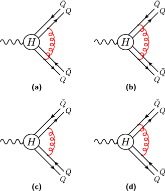
Figure 11: One-gluon corrections to the double-quarkonium production amplitude. The blob labeled $H$ represents the lowest-order hard-scattering process in which two heavy quark-antiquark pairs are created.

In this section we consider double quarkonium production in $e^{+}e^{-}$ annihilation, $\gamma^{*}\to H_{1}(P_{1})+H_{2}(P_{2})$. $H_{1}$ and $H_{2}$ are the produced quarkonium states. For definiteness, we will assume that the produced quarkonia are charmonium states.

Recall that there are QCD and QED contributions to the Born-level hard-scattering process for double-quarkonium production in $e^{+}e^{-}$ annihilation. (See Ref. Braaten:2002fi for details.) However, since this is an exclusive process, only color-singlet $Q\bar{Q}$ pairs can contribute. Therefore, the soft-gluon loop corrections to the QED diagrams are zero at one loop. Nonvanishing corrections to the QED diagrams appear only at two-loop order.

We now write the amplitude as

$$\mathcal{A}_{1}^{\textrm{soft}}=R_{H_{1}+H_{2}}\mathcal{A}_{0}\textrm{C},$$ (60)

where C is the appropriate color factor and $R_{H_{1}+H_{2}}$ is the soft loop factor, which is given by

$$R_{H_{1}+H_{2}}=I(p_{1q},p_{2q})+I(p_{1\bar{q}},p_{2q})+I(p_{1q},p_{2\bar{q}})+I(p_{1\bar{q}},p_{2\bar{q}}).$$ (61)

We obtain $I(p_{1i},p_{2j})$ from Eq. (58). Retaining only those terms with one or fewer factors of $q_{1}$ or $q_{2}$ and discarding terms containing two or more powers of $z=4m_{c}^{2}/s$, we obtain

$$I(p_{1i},p_{2j}) = \frac{\alpha_{s}}{4\pi\epsilon_{\rm IR}}$$

$$\hbox{}\hskip-50.00008pt\times\left[2b_{i}b_{j}\pi i+b_{i}b_{j}\left(2\ln z+4z\right)-4b_{i}\frac{P_{1}\cdot q_{2}}{P_{1}\cdot P_{2}}-4b_{j}\frac{P_{2}\cdot q_{1}}{P_{1}\cdot P_{2}}-8\frac{q_{1}\cdot q_{2}}{P_{1}\cdot P_{2}}+8\frac{P_{1}\cdot q_{2}P_{2}\cdot q_{1}}{(P_{1}\cdot P_{2})^{2}}\right],$$

(62)

where $b_{i}$ is defined in Eq. (56b).

Now let us evaluate the various scalar products that appear in Eq. (62). From Eqs. (20), (22), and (23), we have

$$P_{1}\cdot P_{2} = \frac{1}{2}(s-M_{1}^{2}-M_{2}^{2}),$$ (63a)

$$P_{1}\cdot q_{2} = -\frac{Q}{M_{2}}P_{\rm CM}\hat{q}_{2}^{z},$$ (63b)

$$P_{2}\cdot q_{1} = +\frac{Q}{M_{1}}P_{\rm CM}\hat{q}_{1}^{z},$$ (63c)

$$q_{1}\cdot q_{2} = -\left[(P_{\rm CM}^{2}+E_{1}E_{2})\frac{\hat{q}_{1}^{z}\hat{q}_{2}^{z}}{M_{1}M_{2}}+\bm{q}_{1\perp}\cdot\bm{q}_{2\perp}\right]$$ (63d)

$$= -P_{1}\cdot P_{2}\frac{\hat{q}_{1}^{z}\hat{q}_{2}^{z}}{M_{1}M_{2}}-\bm{q}_{1\perp}\cdot\bm{q}_{2\perp},$$

where

$$P_{\rm CM}^{2}=\frac{1}{4s}[(s-M_{1}^{2}-M_{2}^{2})^{2}-4M_{1}^{2}M_{2}^{2}].$$ (64)

Thus, we see that all of the invariants are of order $Q^{2}=s$ and that the various terms in Eq. (62) are of order $(m_{c}/Q)^{0}$. If we add the contributions of Figs. 11(a) and 11(b) or Figs. 11(c) and 11(d), then the first, second, and third terms in Eq. (62) cancel. Similarly, if we add the contributions of Figs. 11(a) and 11(c) or Figs. 11(b) and 11(d), then the first, second, and fourth terms in Eq. (62) cancel. Therefore, we obtain

$$R_{H_{1}+H_{2}}=\frac{8\alpha_{s}}{\pi\epsilon_{\textrm{IR}}}\left[-\frac{q_{1}\cdot q_{2}}{P_{1}\cdot P_{2}}+\frac{q_{1}\cdot P_{2}q_{2}\cdot P_{1}}{(P_{1}\cdot P_{2})^{2}}\right].$$ (65)

Now,

$$-\frac{q_{1}\cdot q_{2}}{P_{1}\cdot P_{2}} = \frac{\hat{q}_{1}^{z}\hat{q}_{2}^{z}}{M_{1}M_{2}}+\frac{2\bm{q}_{1\perp}\cdot\bm{q}_{2\perp}}{s-M_{1}^{2}-M_{2}^{2}},\hskip 28.45274pt$$ (66a)

$$\frac{q_{1}\cdot P_{2}q_{2}\cdot P_{1}}{(P_{1}\cdot P_{2})^{2}} = -\frac{\hat{q}_{1}^{z}\hat{q}_{2}^{z}}{M_{1}M_{2}}\frac{4sP_{\rm CM}^{2}}{[s-M_{1}^{2}-M_{2}^{2}]^{2}}.$$ (66b)

Therefore, we have

$$R_{H_{1}+H_{2}} = \frac{16\alpha_{s}}{\pi\epsilon_{\textrm{IR}}}\Big{[}\frac{\bm{q}_{1\perp}\cdot\bm{q}_{2\perp}}{s-M_{1}^{2}-M_{2}^{2}}+\hat{q}_{1}^{z}\hat{q}_{2}^{z}\frac{2M_{1}M_{2}}{[s-M_{1}^{2}-M_{2}^{2}]^{2}}\Big{]}$$ (67)

$$\approx \frac{16\alpha_{s}}{\pi\epsilon_{\textrm{IR}}}\frac{\bm{q}_{1\perp}\cdot\bm{q}_{2\perp}}{M^{2}}z\sim\frac{(m_{c}v)^{2}}{s},$$

where we have used the fact that the components of $\bm{q}_{i\perp}$ are of order $m_{c}v$. Equation (67) shows explicitly the suppression of the soft divergence that is expected from the factorization proof.

We can see that the soft divergent terms are proportional to one power of $q_{1}$ and one power of $q_{2}$. Therefore, double-$S$-wave production ($\gamma^{*}\to J/\psi+\eta_{c}$) and $S$-wave/$P$-wave production ($\gamma^{*}\to J/\psi+\chi_{c},$ $\eta_{c}+h_{c}$) at one-loop and at leading order in $v$ are free of soft divergences. This is confirmed by the explicit one-loop calculations of Refs. Zhang:2005cha ; Zhang:2008gp , for the $J/\psi+\eta_{c}$ and $J/\psi+\chi_{c}$ cases.

Note that, if we consider only the contributions from the diagrams of Figs. 11(a) and 11(b) or Figs. 11(c) and 11(d), then the fourth term in Eq. (62) survives. Similarly, if we consider only the contributions from the diagrams of Figs. 11(a) and 11(c) or Figs. 11(b) and 11(d), then the third term in Eq. (62) survives. Each of these terms are of order $(m_{c}/Q)^{0}$. At first sight, this seems puzzling, since we expect soft divergences to cancel up to terms of order $m_{c}/Q$ when we add the contributions from the connections of a soft gluon to the quark and antiquark in a quarkonium. The failure of that cancellation in the present case can be understood because the soft approximation that we have taken contains enhancements that arise when the gluon momentum is nearly collinear to either of the quarkonia momenta. Actual collinear divergences (logarithms of $m_{c}$) are absent in the third and fourth terms in Eq. (62) because, in the one-loop case, they appear with equal strength in the contributions in which the gluon connects to the quark or the antiquark in a quarkonium. However, a residual finite piece of the collinear enhancement survives because the soft approximations for the quark and antiquark lines are not equal when the gluon momentum is in the collinear region. This failure of the soft cancellation when the soft function contains collinear enhancements was noted in Ref. Bodwin:2009cb . In the proof of factorization that we have given, such collinear enhancements are removed from the soft function $S$ and reside in the $J^{\pm}$ functions and associated eikonal lines. In our one-loop example, we have neglected the dependence of the hard function on the momentum of the gluon. Therefore, the $C^{+}$ eikonal lines that arise from the $C^{+}$ enhancements in the diagrams of Figs. 11(a) and 11(c) or Figs. 11(b) and 11(d) cancel, and the $C^{-}$ eikonal lines that arise from the $C^{-}$ enhancements in the diagrams of Figs. 11(a) and 11(b) or Figs. 11(c) and 11(d) cancel. The sum of all four diagrams in Fig. 11 is therefore free of collinear enhancements that could spoil the soft cancellation and is in accord with the results of the factorization proof.

IV.3 $\bm{B}$-meson decays

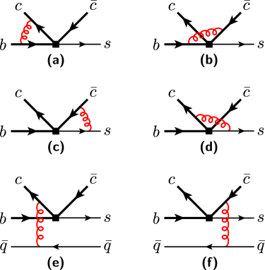
Figure 12: One-gluon corrections to the lowest-order $B$ decay amplitude. The black square represents the electroweak interaction.

In this section we consider decay of a $B$ meson into a light meson plus a charmonium state. For definiteness, we take the light meson to be a $K$ meson. Therefore we have the process $B(p_{B})\to H(P_{1})+K(p_{K})$. $H$ is the produced charmonium state, which we take to be a ${}^{3}P_{J}$ state. The one-soft-gluon corrections to the lowest-order decay amplitude are represented in Fig. 12. We refer to diagrams (a)–(d) as vertex corrections and to diagrams (e) and (f) as spectator contributions.

IV.3.1 Vertex corrections

In discussing soft contributions to the vertex corrections, we assume that the light quark has a small mass $m_{s}$, and we work in the limit $m_{s}\to 0$. In order to make contact with the results in Ref. Song:2003yc , we neglect $q_{k}=-yp_{K}+p_{k_{q}}$ in comparison with $p_{K}$, and we neglect $\bm{q}_{B}\sim\Lambda_{\rm QCD}$ in comparison with $m_{b}$. We keep terms containing zero or one power of $q_{1}$.

For the vertex corrections in which the soft gluon attaches to the light-quark line [Figs.12(c) and 12(d)], we obtain

$$\bar{\beta}\Big{(}p_{k_{q}},p_{1q(\bar{q})}\Big{)}=1-8\frac{m_{c}^{2}m_{s}^{2}}{y^{2}\left(m_{b}^{2}-4m_{c}^{2}\right)^{2}}\left(1\mp 8\frac{p_{b}\cdot q_{1}}{m_{b}^{2}-4m_{c}^{2}}\right).$$ (68)

The upper sign corresponds to the quark with momentum $p_{1q}$, and the lower sign corresponds to the antiquark with momentum $p_{1\bar{q}}$. The soft loop factor is then given by

$$I\left(p_{k_{q}},p_{1q(\bar{q})}\right)=\pm\frac{\alpha_{s}}{4\pi\epsilon_{\textrm{IR}}}\left[\ln\left(8\frac{m_{c}^{2}m_{s}^{2}}{y^{2}\left(m_{b}^{2}-4m_{c}^{2}\right)^{2}}\right)\mp 8\frac{p_{b}\cdot q_{1}}{\left(m_{b}^{2}-4m_{c}^{2}\right)}+2\pi i\right].$$ (69)

This expression contains collinear divergences, which manifest themselves when we take $m_{s}=0$. The divergences arise because the soft expressions contain contributions from $C^{-}$ momentum. However, as we have explained in Sec. IV.2, at one-loop order, the collinear divergences cancel when one sums over the connections to the quark and the antiquark in the charmonium. Computing that sum, we obtain

$$I\left(p_{k_{q}},p_{1q}\right)+I\left(p_{k_{q}},p_{1\bar{q}}\right)=-\frac{16\alpha_{s}}{4\pi\epsilon_{\textrm{IR}}}\frac{p_{b}\cdot q_{1}}{\left(m_{b}^{2}-4m_{c}^{2}\right)}=-\frac{16\alpha_{s}}{4\pi\epsilon_{\textrm{IR}}}\frac{p_{b}\cdot q_{1}}{m_{b}^{2}\left(1-z\right)},$$ (70)

where, again, $z=4m_{c}^{2}/m_{b}^{2}$.

For the vertex corrections in which the soft gluon attaches to the $b$-quark line [Figs. 12(a) and 12(b)], we obtain

$$\bar{\beta}\Big{(}p_{b},p_{1q(\bar{q})}\Big{)}=\beta_{1}(1\pm\delta_{1}),$$ (71)

with

$$\beta_{1}=\frac{m_{b}^{2}-4m_{c}^{2}}{m_{b}^{2}+4m_{c}^{2}},\;\delta_{1}=\frac{64m_{c}^{2}m_{b}^{2}p_{b}\cdot q_{1}}{(m_{b}^{2}+4m_{c}^{2})(m_{b}^{2}-4m_{c}^{2})^{2}}.$$ (72)

The corresponding soft loop factors are given by

$$I\Big{(}p_{b},p_{1q(\bar{q})}\Big{)} = \frac{\alpha_{s}}{4\pi\epsilon_{\textrm{IR}}}\!\left\{\pm\frac{1}{\beta_{1}}\ln\left(\frac{1+\beta_{1}}{1-\beta_{1}}\right)\right.$$

$$\left.+\frac{\delta_{1}}{\beta_{1}}\!\!\left[\!\ln\!\left(\frac{1-\beta_{1}}{1+\beta_{1}}\right)\!+\frac{2\beta_{1}}{1-\beta_{1}^{2}}\right]\right\}\!.$$

Summing over both diagrams in Figs. 12(a) and 12(b), we obtain

$$I\left(p_{b},p_{1q}\right)+I\left(p_{b},p_{1\bar{q}}\right) = \frac{2\alpha_{s}}{4\pi\epsilon_{\textrm{IR}}}\frac{\delta_{1}}{\beta_{1}}\left[\!\ln\!\left(\frac{1-\beta_{1}}{1+\beta_{1}}\right)\!+\frac{2\beta_{1}}{1-\beta_{1}^{2}}\right]$$ (74)

$$= \frac{16\alpha_{s}}{4\pi\epsilon_{\textrm{IR}}}\frac{p_{b}\cdot q_{1}}{m_{b}^{2}}\frac{2z}{(1-z)^{3}}\left(\ln z+\frac{1-z^{2}}{2z}\right).$$

As we have explained in Sec. IV.2, it is necessary to add the contributions of all four diagrams in order obtain the suppression of the infrared-divergent terms because the soft expressions contain $C^{+}$ contributions that spoil the soft cancellation. Those $C^{+}$ contributions, which correspond to $C^{+}$ eikonal lines in the general factorization proof, cancel at one-loop order when one sums over the connections to the $b$ quark and the light quark. When we add the contributions of all four diagrams, i.e., Eqs. (70) and (74), the leading term does indeed cancel, and we obtain

$$I\left(p_{k_{q}},p_{1q}\right)+I\left(p_{k_{q}},p_{1\bar{q}}\right)+I\left(p_{b},p_{1q}\right)+I\left(p_{b},p_{1\bar{q}}\right)=\frac{16\alpha_{s}}{4\pi\epsilon_{\textrm{IR}}}\frac{p_{b}\cdot q_{1}}{m_{b}^{2}}2z\frac{1-z+\ln z}{(1-z)^{3}}.$$ (75)

The remaining infrared-divergent terms are suppressed at least as $z\ln z$. We generally expect a suppression of the factorization-violating contributions by only a factor $\sqrt{z}$. However, as we have mentioned in Sec. III.11, the suppression factor can become $z$ for production of $P$-wave quarkonia if one neglects the transverse momenta of the constituents of the $B$ meson and the light meson, as we are doing in the present example. As was noted in Ref. Song:2003yc , the expression in Eq. (75) gives a nonvanishing contribution to the production of a ${}^{3}P_{J}$ charmonium only if $J=0$ or $J=2$. The Born-level cross section to produce a ${}^{3}P_{J}$ charmonium with $J=0$ or $J=2$ vanishes, and so the violations of factorization are suppressed only as $z\ln z/\alpha_{s}$ with respect to the leading factorizing terms.

Finally, we mention that, when we include the Born factors in the amplitude, along with the soft factor, and decompose $q_{1}$ and the quarkonium spin polarization $\epsilon^{\star}$ into the $J=0$ and $J=2$ angular-momentum tensors, then we obtain agreement with the results in Eqs. (14) and (16) of Ref. Song:2003yc .

IV.3.2 Spectator contributions

In the spectator contributions of Figs. 12(e) and 12(f), we initially assume that $p_{l}$, $q_{k}$ and $\bar{y}p_{K}$ are all of order $\Lambda_{\rm QCD}$. Then, because the gluon in Figs. 12(e) and 12(f) carries momentum $p_{k_{\bar{q}}}-p_{l}\sim\Lambda_{\rm QCD}$, the heavy-quark or heavy-antiquark propagator is off shell by order $m_{b}\Lambda_{\rm QCD}$. That is, its momentum is in the semihard region. Therefore, in this example, we are discussing the further factorization of the gluons with endpoint soft momenta that was described in Sec. III.10.2. Eventually, we wish to make contact with the results in Ref. Song:2003yc . In that work, $q_{k}=\bar{y}p_{K}-p_{k_{\bar{q}}}$ was neglected in comparison with $\bar{y}p_{K}$. Neglecting $q_{k}$ generates endpoint divergences in $\bar{y}$ that are cut off in our model when $\bar{y}p_{K}\sim q_{k}\sim\Lambda_{\rm QCD}$. Our discussion in this example also applies to the cancellation of those endpoint divergences.

Since the gluon in Figs. 12(e) and 12(f) carries momentum of order $\Lambda_{\rm QCD}$ or less, we can apply the soft approximation to the connections of the gluon to the heavy-quark and heavy-antiquark lines. Keeping terms up to order $q_{1}$, we find that the soft factor for the heavy quark and antiquark lines for sum of the diagrams in Figs. 12(e) and 12(f) is

$$S_{\mu}=\frac{1}{(p_{k_{\bar{q}}}-p_{l})^{2}}\frac{4}{P_{1}\cdot(p_{k_{\bar{q}}}-p_{l})}q_{\mu}^{\prime},$$ (76)

where

$$q^{\prime}=q_{1}-P_{1}\frac{q_{1}\cdot(p_{k_{\bar{q}}}-p_{l})}{P_{1}\cdot(p_{k_{\bar{q}}}-p_{l})},$$ (77)

and we have included the factor $1/(p_{k_{\bar{q}}}-p_{l})^{2}$ from the gluon propagator in $S_{\mu}$. We note that $S_{\mu}$ is proportional to $q\sim m_{c}v$. We will concern ourselves only with the contributions to the production a $P$-wave quarkonium at leading order in $v$. Therefore, we can retain only terms of leading order in $v$ in the remaining factors that are associated with the heavy quarkonium.

In computing the remaining factors in the spectator amplitudes, we make use of the quark-antiquark spin-projection operators that are given in the Appendix. In the projector for heavy quark and antiquark, we take the spin-triplet case, which corresponds to the calculation for the $\chi_{cJ}$ in Ref. Song:2003yc . The projector for a charm-quark pair production can be obtained by setting $m_{q}=m_{\bar{q}}=m_{c}$ and $E_{q}+E_{\bar{q}}=2\sqrt{m_{c}^{2}+\hat{\bm{q}}_{i}^{2}}$ in Eq. (100b). Retaining only the terms of leading order in $v$ and using relativistic normalization, we have

$$\bar{\Pi}_{3}^{\rm onium}\approx-\frac{1}{2\sqrt{2}}\,\epsilon\!\!\!/^{\star}(/\!\!\!\!P_{1}+2m_{c}).$$ (78)

We obtain the $B$-meson projector by setting $m_{q}=m_{b}$, $E_{q}=m_{b}$, $m_{\bar{q}}=m_{l}$, and $E_{\bar{q}}=E_{l}$ in Eq. (97) and retaining the terms of leading order in $\Lambda_{\rm QCD}$. Using relativistic normalization, we have

$$\Pi_{1}^{B}\approx C_{B}(p\!\!\!/_{b}+m_{b})\gamma_{5}\left(1-\frac{p\!\!\!/_{l}}{m_{l}}\right),$$ (79)

where the light-antiquark mass $m_{l}$ is of order $\Lambda_{\rm QCD}$ and the factor $C_{B}$ is defined by

$$C_{B}=\frac{1}{2}\sqrt{\frac{m_{l}}{m_{b}(1+E_{l}/m_{l})}}.$$ (80)

Similarly, we obtain the $K$-meson projector by retaining the terms in Eq. (100a) of leading order in $\Lambda_{\rm QCD}$. Using relativistic normalization, we have

$$\Pi_{1}^{K}\approx C_{K}\left\{\left[1+\left(\frac{m_{\bar{q}}}{m_{q}}-1\right)y\right]p\!\!\!/_{K}\gamma_{5}-\frac{1}{m_{q}}p\!\!\!/_{K}q\!\!\!/_{k}\gamma_{5}\right\},$$ (81)

where we have retained small masses $m_{q}$ and $m_{\bar{q}}$ of order $\Lambda_{\rm QCD}$ for the quark and antiquark, respectively. The coefficient $C_{K}$ is defined by

$$C_{K}=\frac{m_{q}(E_{q}+m_{q}+E_{\bar{q}}+m_{\bar{q}})}{2\sqrt{2(E_{q}+m_{q})(E_{\bar{q}}+m_{\bar{q}})}(E_{q}+E_{\bar{q}})}.$$ (82)

Now, the trace over the heavy quark and antiquark lines is

$$U_{\rho}={\rm Tr}[\Pi_{3}^{\rm onium}\gamma_{\rho}(1-\gamma_{5})]\approx-2\sqrt{2}m_{c}\epsilon^{\star}_{\rho}.$$ (83)

The factor $\gamma_{\rho}(1-\gamma_{5})$ comes from the $V-A$ weak vertex. The trace over the $B$-meson and light-meson quark and antiquark lines is

$$L_{\rho}^{\mu} = \mathrm{Tr}\left[\Pi_{1}^{K}\gamma_{\rho}\left(1-\gamma_{5}\right)\Pi_{1}^{B}\gamma^{\mu}\right]$$ (84)

$$\approx C_{B}C_{K}\mathrm{Tr}\left[\left(p\!\!\!/_{K}\gamma_{5}-\frac{1}{m}p\!\!\!/_{K}q\!\!\!/_{k}\gamma_{5}\right)\gamma_{\rho}\left(1-\gamma_{5}\right)\left(p\!\!\!/_{b}+m_{b}\right)\gamma_{5}\left(1-\frac{p\!\!\!/_{l}}{m}\right)\gamma^{\mu}\right],$$

where the factor $\gamma_{\rho}(1-\gamma_{5})$ comes from the $V-A$ weak vertex, and, for simplicity, we have set $m_{q}=m_{\bar{q}}=m_{l}=m$. The complete amplitude corresponding to the diagrams in Figs. 12(e) and 12(f) is

$$A^{\rm spectator} = \frac{-ig^{2}C_{F}C_{\rm EW}}{N_{c}^{3/2}}S_{\mu}U^{\rho}L_{\rho}^{\mu}$$ (85)

$$\approx \frac{-ig^{2}C_{F}C_{B}C_{K}C_{\rm EW}}{N_{c}^{3/2}}\frac{8\sqrt{2}m_{c}}{(p_{l}-p_{k_{\bar{q}}})^{2}P_{1}\cdot(p_{k_{\bar{q}}}-p_{l})}$$

$$\times\mathrm{Tr}\left[\left(-p\!\!\!/_{K}\gamma_{5}+\frac{p\!\!\!/_{K}q\!\!\!/_{k}\gamma_{5}}{m}\right)\epsilon\!\!\!/^{*}\left(1-\gamma_{5}\right)\left(p\!\!\!/_{b}+m_{b}\right)\gamma_{5}\left(1-\frac{p\!\!\!/_{l}}{m}\right)q\!\!\!/^{\prime}\right].$$

Here, $C_{\rm EW}=(G_{F}/\sqrt{2})[V_{cb}V_{cs}^{*}C_{1}-V_{tb}V_{ts}^{*}(C_{4}+C_{6})]$, where $G_{F}$ is the Fermi constant, the $V_{q_{1}q_{2}}$ are the CKM matrix elements, and the $C_{i}$ are the Wilson coefficients of the effective electroweak Hamiltonian. (See, for example, Ref. Song:2003yc for details.)

In Eq. (85), the terms proportional to the spatial components of $p_{l}$ vanish upon integration over the angles that are associated with those spatial components. Then, using the fact that $\gamma_{0}\approx p\!\!\!/_{b}/m_{b}$, up to terms of relative order $\Lambda_{\rm QCD}/m_{b}$, we can write

$$A^{\rm spectator} \approx \frac{-ig^{2}C_{F}C_{B}(1+E_{l}/m)C_{K}C_{\rm EW}}{N_{c}^{3/2}}\frac{8\sqrt{2}m_{c}}{(p_{k_{\bar{q}}}-p_{l})^{2}P_{1}\cdot(p_{k_{\bar{q}}}-p_{l})}$$ (86)

$$\times\mathrm{Tr}\left[\left(-p\!\!\!/_{K}\gamma_{5}+\frac{p\!\!\!/_{K}q\!\!\!/_{k}\gamma_{5}}{m}\right)\epsilon\!\!\!/^{*}\left(1-\gamma_{5}\right)(p\!\!\!/_{b}+m_{b})\gamma_{5}q\!\!\!/^{\prime}\right].$$

The gamma-matrix factors in this expression that are associated with the $B$ meson correspond to the leading-twist $B$-meson light-cone $\Phi_{B1}$ in Eq. (I). Expanding terms inside the trace, we have

$$A^{\rm spectator} \approx \frac{-ig^{2}C_{F}C_{B}(1+E_{l}/m)C_{K}C_{\rm EW}}{N_{c}^{3/2}}\frac{8\sqrt{2}m_{c}}{(p_{k_{\bar{q}}}-p_{l})^{2}P_{1}\cdot(p_{k_{\bar{q}}}-p_{l})}$$ (87)

$$\times\left\{-\mathrm{Tr}\left[p\!\!\!/_{K}\epsilon\!\!\!/^{*}\left(1-\gamma_{5}\right)p\!\!\!/_{b}q\!\!\!/^{\prime}\right]-(m_{b}/m)\mathrm{Tr}\left[p\!\!\!/_{K}q\!\!\!/_{k}\epsilon\!\!\!/^{*}\left(1-\gamma_{5}\right)q\!\!\!/^{\prime}\right]\right\}$$

$$\equiv \frac{-ig^{2}C_{F}C_{B}(1+E_{l}/m)C_{K}C_{\rm EW}}{N_{c}^{3/2}}\frac{8\sqrt{2}m_{c}}{(p_{k_{\bar{q}}}-p_{l})^{2}P_{1}\cdot(p_{k_{\bar{q}}}-p_{l})}(T_{1}+T_{2}).$$

In evaluating the sizes of the contributions to $A^{\rm spectator}$, we make use of the orders of magnitude of the components of the various four vectors in the $B$-meson rest frame. Some of these are given in Eqs. (15a), (18), (25), and (88). In the case of $q^{\prime}$, we see from Eq. (22) that, in the $B$-meson rest frame,

$$(q^{\prime})^{+} \sim vm_{c},$$ (88a)

$$(q^{\prime})^{-} \sim vm_{c}^{2}/m_{b},$$ (88b)

$$\bm{q}^{\prime}_{\perp} \sim vm_{c}.$$ (88c)

This is in contrast with either $P$ or $q$, which, as can be seen from Eq. (25), have plus components that are of order $m_{b}$ and $vm_{b}$, respectively. The suppression of the plus component of $q^{\prime}$ is a consequence of the soft cancellation.

Now consider the contribution of $T_{1}$ in Eq. (87). $T_{1}$ comes from the $-p\!\!\!/_{K}\gamma_{5}$ term in the first parenthesis in Eq. (86), which corresponds to the leading-twist light-meson light-cone distribution. The contribution of $T_{1}$ is proportional to the one that was considered in Ref. Song:2003yc . Evaluating the trace in $T_{1}$, we obtain

$$T_{1}=-4\left(p_{K}\cdot\epsilon^{\star}p_{b}\cdot q^{\prime}-p_{K}\cdot p_{b}\epsilon^{\star}\cdot q^{\prime}+p_{K}\cdot q^{\prime}\epsilon^{\star}\cdot p_{b}-i\epsilon^{\alpha\rho\beta\mu}p_{k\alpha}\epsilon^{\star}_{\rho}p_{b\beta}q_{\mu}^{\prime}\right),$$ (89)

where we have used the convention $\textrm{Tr}[\gamma_{5}/\!\!\!a/\,\!\!\!b\,/\!\!\!c\,/\!\!\!d]=4i\epsilon_{\alpha\beta\gamma\delta}a^{\alpha}b^{\beta}c^{\gamma}d^{\delta}$, with $\epsilon_{0123}=-\epsilon^{0123}=1$. It is now easily seen that the terms in Eq. (89) are of order $vm_{b}^{3}$, $vm_{c}m_{b}^{2}$, $vm_{b}^{3}$, and $vm_{c}m_{b}^{2}$, respectively. We can compare this contribution with the individual contributions that appear before we apply the soft cancellation or with the contributions in which the gluon in Figs. 12(e) and 12(f) attaches at its upper end to the quark lines from the $B$ meson or the $K$ meson. In the cancelling contributions, $q^{\prime}$ in $T_{1}$ is replaced with $P$, and $T_{1}$ becomes of order $m_{b}^{4}/m_{c}$. Thus, we see that Eq. (89) is suppressed as $vm_{c}/m_{b}$ relative to the cancelling contributions, in agreement with what we expect for the soft cancellation from the general factorization proof. In the contributions in which the gluon in Figs. 12(e) and 12(f) attaches at its upper end to the quark lines from the $B$ meson or the $K$ meson, which are factorizing contributions that contribute to the $B$-meson-$K$-meson form factor, $q^{\prime}$ in $T_{1}$ is replaced with $p_{b}$ or $p_{K}$. With this replacement, $T_{1}$ is again of order $m_{b}^{4}/m_{c}$. However, as we have mentioned, the Born-level factorizing contributions to the production of a ${}^{3}P_{J}$ charmonium with $J=0$ or $J=2$ vanish, and so the contributions of Eq. (89) are suppressed as $m_{c}v/(\alpha_{s}m_{b})$ relative to the leading factorizing contributions.

Next consider the contribution of $T_{2}$ in Eq. (87), which comes from the $p\!\!\!/_{K}q\!\!\!/_{k}\gamma_{5}/m$ term in the first parenthesis in Eq. (86). The leading contributions in $T_{2}$ are of order $vm_{b}^{3}$ and are suppressed by a factor $m_{c}v/(\alpha_{s}m_{b})$ relative to the factorizing terms. However, the leading contributions in $T_{2}$ are proportional to the transverse components of $q_{k}$. Upon integration of $T_{2}$ over the angles of the transverse components of $q_{k}$, these leading contributions vanish. From Eq. (18), we see that the minus component of $q_{k}$ vanishes and that the plus component of $q_{k}$ is suppressed by a factor $\Lambda_{\rm QCD}/m_{b}$ relative to the transverse components. Hence, the contributions of $T_{2}$ are suppressed by a factor $\Lambda_{\rm QCD}m_{c}v/(\alpha_{s}m_{b}^{2})$ relative to the factorizing terms, and are negligible in comparison with the other factorization-violating contributions.

Now let us retain only the leading contribution to $A^{\rm spectator}$, which is proportional to $T_{1}$. As we have mentioned, this contribution is the one that was considered in Ref. Song:2003yc . In that calculation, light-quark masses were taken to be zero, $q_{k}=\bar{y}p_{K}-p_{k_{\bar{q}}}$ was neglected in comparison with $\bar{y}p_{K}$, and $p_{l}$ was taken to have only a plus component, which is written as $p_{l}^{+}=\xi p_{B}^{+}\approx\xi p_{b}^{+}$. Under these assumptions, $p_{k_{\bar{q}}}=\bar{y}p_{K}$, which has only a minus component that is nonzero, $q^{\prime}=q_{1}-P_{1}(q_{1}\cdot p_{K})/(P_{1}\cdot p_{K})$, and $(q^{\prime})^{+}=0$. Then, the resulting contribution is

$$A^{\rm spectator} \approx \frac{-ig^{2}C_{F}C_{B}(1+E_{l}/m)C_{K}C_{\rm EW}}{N_{c}^{3/2}}\frac{16\sqrt{2}m_{c}}{\xi\bar{y}^{2}p_{K}\cdot p_{b}P_{1}\cdot p_{K}}$$ (90)

$$\times\left(p_{K}\cdot\epsilon^{\star}p_{b}\cdot q^{\prime}-p_{K}\cdot p_{b}\epsilon^{\star}\cdot q^{\prime}-i\epsilon^{\alpha\rho\beta\mu}p_{k\alpha}\epsilon^{\star}_{\rho}p_{b\beta}q_{\mu}^{\prime}\right),$$

which yields an endpoint divergence, owing to the factor $\bar{y}^{2}$ in the denominator. The terms in parentheses in Eq. (90) are all of order $vm_{c}m_{b}^{2}$. That is, there is a suppression factor, relative to the cancelling terms, of order $m_{c}^{2}/m_{b}^{2}$. From the arguments of Sec. III.11, we expect such a suppression because we are neglecting the transverse momenta of the constituents of the $B$ meson and the light meson. In order to make contact with the calculation of Ref. Song:2003yc , we make the replacements $C_{B}(1+E_{l}/m)\to(-i/4)f_{B}\Phi_{B}(\xi)$ and $C_{K}\to(i/4)f_{K}\Phi_{K}(y)$, multiply by a factor $\sqrt{2m_{\chi_{c}}/(2m_{c})^{2}}\approx\sqrt{1/m_{c}}$ to compensate for the normalization of the quarkonium state relative to the normalizations of the quark and antiquark states, multiply by a $P$-wave quarkonium spatial wave function, and integrate over the wave-function momentum. Then, decomposing $q$ and $\epsilon^{\star}$ into $J=0$ and $J=2$ angular-momentum tensors, we obtain agreement between Eq. (90) and the divergent terms in Eqs. (15) and (17) of Ref. Song:2003yc . We find in the $J=1$ case that

$$f_{\rm II}=-\frac{4\sqrt{2}\epsilon^{*}\cdot p_{b}z}{m_{b}^{2}(1-z)^{2}}\int_{0}^{1}d\xi\,\frac{\Phi_{B}(\xi)}{\xi}\,\int_{0}^{1}dy\,\frac{\Phi_{K}(y)}{\bar{y}^{2}},$$ (91)

where $f_{\rm II}$ is defined in Ref. Song:2003yc and we have retained only the infrared-divergent terms.

V Summary and Discussion

In this paper, we have given detailed proofs, valid to all orders in $\alpha_{s}$, of factorization theorems for two exclusive quarkonium-production processes: the production of two quarkonia in $e^{+}e^{-}$ annihilation and the production of a charmonium and a light-meson in $B$-meson decays. We have supplemented our proofs with one-loop examples of the factorization and cancellation of soft singularities. (See Sec. IV.) Proofs of these factorization theorems were sketched in Ref. Bodwin:2008nf . In the present paper, we have provided more detailed arguments. The proofs in Ref. Bodwin:2008nf did not consider the possibility that on-shell lines could emit gluons with arbitrarily small momenta. Such a possibility arises, for example, when one computes short-distance coefficients by making use of on-shell matching conditions. In the present paper, we have shown that factorization still holds when one takes into account this possibility. We have also given more refined estimates of the violations of factorization than were given in Ref. Bodwin:2008nf , by considering the dependence of such violations on the velocity $v$ of the heavy quark or antiquark in the quarkonium rest frame. We note that, although our proofs are demonstrated in models in which external lines are taken to be on the mass shell, the methods of these proofs would apply to off-shell models as well, provided that the models maintain gauge invariance.

In the proofs of factorization, our general strategy has been to identify soft singularities, collinear singularities, and would-be collinear singularities that appear in the limit of zero heavy-quark mass. By demonstrating the factorization of these singularities and would-be singularities, we are able to argue that the associated logarithmic enhancements also factorize. Once the logarithmic enhancements have been removed, the remainder of the production amplitude can depend only on the hard scale and, hence, is perturbatively calculable.

In demonstrating the factorization of singularities and would-be singularities, we have made use of standard techniques (see, for example, Refs. Sterman:1978bi ; Sterman:1978bj ; Collins:1985ue ; Collins:1989gx ), but we have had to augment them in order to deal with the situation in which low-energy collinear gluons attach to soft gluons. For this purpose, we made use of the approach developed in Ref. Bodwin:2009cb in the context of the production of light mesons in $e^{+}e^{-}$ annihilation. The methods of proof that we have given here should, generally, be applicable to proofs of factorization for other exclusive processes in QCD.

Our factorized form for exclusive production of two quarkonia in $e^{+}e^{-}$ annihilation is given in Eq. (1). The expression in Eq. (1) has been used in leading-order and next-to-leading-order calculations of exclusive double-charmonium production. It is generally referred to as the “NRQCD factorization” formula.

Our factorized form for the exclusive production of a charmonium and a light meson in $B$ decays is given in Eq. (2). An expression of the form in Eq. (2) was suggested in Ref. Beneke:2000ry on the basis of an analysis of $B$-meson decays to light mesons. (In Ref. Beneke:2000ry , the factorized form was written in terms of the quarkonium light-cone distribution, rather than in terms of NRQCD matrix elements.) In Ref. Beneke:2000ry , it was conjectured that the violations of factorization should vanish in the limit $m_{c}\to 0$, but a detailed analysis of the scaling of the violations of factorization with $m_{c}$, $m_{b}$, and $v$ was not given.

We find, generally, that the violations of factorization are suppressed by a factor $f_{i}=m_{c}v^{2}/Q$ for each charmonium $i$ in an $S$-wave state and by a factor $f_{i}=m_{c}/Q$ for each charmonium $i$ in a higher orbital-angular-momentum state, where $Q=\sqrt{s}$ is the CM energy in $e^{+}e^{-}$ annihilation and $Q=m_{B}$ in $B$-meson decays. Because the violations of factorization are proportional to $v$, they vanish (up to corrections that are proportional to $\Lambda_{\rm QCD}/Q$) if one works to order $v^{0}$ in one charmonium. This statement has been confirmed in calculations at order $\alpha_{s}$ (Refs. Chay:2000xn ; Zhang:2008gp ).

In the case of $B$-meson decays, the error-suppression factors for $S$-wave and $P$-wave charmonia are $f_{i}=v^{2}m_{c}/m_{b}$ and $f_{i}=m_{c}/m_{b}$, respectively. These are not particularly small, and the violations of factorization may well be comparable to the factorized contributions. In the case of $e^{+}e^{-}$ annihilation, the error-suppression factors are smaller by a factor $m_{b}/\sqrt{s}$ than in the case of $B$-meson decays. Furthermore, there is a suppression factor for each quarkonium in the process. Hence, in the case of $e^{+}e^{-}$ annihilation, the errors are likely to be sufficiently small that the factorization formula would be useful. Since the coefficients of the suppression factors are nonperturbative quantities, their sizes must be determined, at present, through phenomenological studies.

In special cases, the relative sizes of the violations of factorization may be enhanced because of quantum-number considerations. For example, in $B$-meson decays, the production of ${}^{3}P_{0}$ or ${}^{3}P_{2}$ charmonia through factorized contributions is not allowed in order $\alpha_{s}^{0}$. The production of ${}^{3}P_{0}$ or ${}^{3}P_{2}$ charmonia through factorization-violating contributions does occur in order $\alpha_{s}^{0}$. Therefore, in these cases, the violations of factorization are enhanced by a factor $1/\alpha_{s}$ relative to the factorized contributions.

Finally, we mention that we could have written the collinear functions $\bar{J}^{\pm}$ that are associated with each quarkonium in terms of light-cone distributions instead of NRQCD matrix elements. As we have explained in Sec. III.11, such an approach yields a hard-scattering function $\tilde{H}$ that is manifestly free of soft divergences. In contrast, in the factorized expressions involving NRQCD matrix elements that we have presented, power-suppressed soft divergences do appear in $\tilde{H}$ and must be discarded. In the case of double-charmonium production, these soft divergences are suppressed as $f_{i}f_{j}$, while the corrections to the light-cone-distribution factorization formula are suppressed only as $f_{i}+f_{j}$. Therefore, in the case of double-charmonium production, the factorized expression involving NRQCD matrix elements that we have presented is more accurate than a factorized expression involving light-cone distributions for the quarkonia.

Appendix A Spin projectors

In this appendix we derive quark-antiquark spin projectors for the case in which the quark and antiquark have different masses. We take the momentum of the quark to be $p_{q}$ and the momentum of the antiquark to be $p_{\bar{q}}$, with both the quark and the antiquark on shell: $p_{q}^{2}=m_{q}^{2}$, $p_{\bar{q}}^{2}=m_{\bar{q}}^{2}$. Therefore, in the quark-antiquark CM frame we have

$$\hat{p}_{q} = (E_{q},+\hat{\bm{q}}),$$ (92a)

$$\hat{p}_{\bar{q}} = (E_{\bar{q}},-\hat{\bm{q}}),$$ (92b)

where $E_{q}=\sqrt{m_{q}^{2}+\hat{\bm{q}}^{2}}$, $E_{\bar{q}}=\sqrt{m_{\bar{q}}^{2}+\hat{\bm{q}}^{2}}$, and $\hat{\bm{q}}$ is the quark three-momentum in the CM frame. It follows that

$$p_{q} = \frac{E_{q}}{E_{q}+E_{\bar{q}}}P+q,$$ (93a)

$$p_{\bar{q}} = \frac{E_{\bar{q}}}{E_{q}+E_{\bar{q}}}P-q,$$ (93b)

where $P=p_{q}+p_{\bar{q}}$ and, in the CM frame, $P$ and $q$ are given by

$$\hat{P} = (M,\bm{0}),$$ (94a)

$$\hat{q} = (0,\hat{\bm{q}}),$$ (94b)

where $M=E_{q}+E_{\bar{q}}$.

The quark and antiquark spinors are given by

$$u(p_{q},s_{q}) = N_{q}\begin{pmatrix}(E_{q}+m_{q})\xi(s_{q})\\ \bm{q}\cdot\bm{\sigma}\xi(s_{q})\end{pmatrix},$$ (95a)

$$v(p_{\bar{q}},s_{\bar{q}}) = N_{\bar{q}}\begin{pmatrix}-\bm{q}\cdot\bm{\sigma}\eta(s_{\bar{q}})\\ (E_{\bar{q}}+m_{\bar{q}})\eta(s_{\bar{q}})\end{pmatrix},$$ (95b)

where the normalization factors are

$$N_{i}=\left\{\begin{array}[]{l}{[2E_{i}(E_{i}+m_{i})]}^{-\frac{1}{2}}\textrm{nonrelativistic},\\ {[E_{i}+m_{i}]}^{-\frac{1}{2}}\textrm{relativistic},\end{array}\right.,$$ (96)

for $i=q$ or $\bar{q}$. Here, $\xi(s_{q})$ and $\eta(s_{\bar{q}})$ are the two-component spinors for the spin states $s_{q}$ and $s_{\bar{q}}$, respectively, with $\eta$ in a representation that is conjugate to that of $\xi$. It then follows straightforwardly that the spin-singlet projector is given by

$$\Pi_{1}(p_{q},m_{q},p_{\bar{q}},m_{\bar{q}}) = \sum_{s_{q},s_{\bar{q}}}u(p_{q},s_{q})\bar{v}(p_{\bar{q}},s_{\bar{q}})\langle\textstyle{\frac{1}{2}}s_{q},\textstyle{\frac{1}{2}}s_{\bar{q}}|00\rangle$$ (97)

$$= -\frac{N_{q}N_{\bar{q}}}{2(E_{q}+E_{\bar{q}})\sqrt{2}}(p\!\!\!/_{q}+m_{q})(P\!\!\!\!/+E_{q}+E_{\bar{q}})\gamma_{5}(p\!\!\!/_{\bar{q}}-m_{\bar{q}})$$

$$= -\frac{\left(E_{q}+m_{q}+E_{\bar{q}}+m_{\bar{q}}\right)N_{q}N_{\bar{q}}}{2\sqrt{2}(E_{q}+E_{\bar{q}})}\,(p\!\!\!/_{q}+m_{q})\gamma_{5}(p\!\!\!/_{\bar{q}}-m_{\bar{q}}),$$

and the spin-triplet projector is given by

$$\Pi_{3}(p_{q},m_{q},p_{\bar{q}},m_{\bar{q}},\lambda) = \sum_{s_{q},s_{\bar{q}}}u(p_{q},s_{q})\bar{v}(p_{\bar{q}},s_{\bar{q}})\langle\textstyle{\frac{1}{2}}s_{q},\textstyle{\frac{1}{2}}s_{\bar{q}}|1\lambda\rangle$$ (98)

$$= \frac{N_{q}N_{\bar{q}}}{2(E_{q}+E_{\bar{q}})\sqrt{2}}(p\!\!\!/_{q}+m_{q})(P\!\!\!\!/+E_{q}+E_{\bar{q}})\,/\!\!\!\epsilon\,(\lambda)(p\!\!\!/_{\bar{q}}-m_{\bar{q}}),$$

where $\epsilon(\lambda)$ is the polarization vector of the spin-triplet state whose components in the quarkonium rest frame are

$$\bm{\epsilon}(\pm) = \mp\frac{1}{\sqrt{2}}(1,\pm i,0),$$ (99a)

$$\bm{\epsilon}(0) = (0,0,1).$$ (99b)

The results in Eqs. (97) and (98) are equivalent, in the equal-mass case to those in Ref. Bodwin:2002hg .

Note that the spin projectors $\Pi_{i}$ in Eqs. (97) and (98) are for the decay of a $q\bar{q}$ pair. The projectors $\bar{\Pi}_{i}$ for the production of a $q\bar{q}$ pair can be obtained in a similar manner as

$$\bar{\Pi}_{1}(p_{q},m_{q},p_{\bar{q}},m_{\bar{q}}) = \sum_{s_{q},\,s_{\bar{q}}}\langle\tfrac{1}{2}\,s_{q},\,\tfrac{1}{2}\,s_{\bar{q}}|00\rangle v(p_{\bar{q}},s_{\bar{q}})\bar{u}(p_{q},s_{q})$$ (100a)

$$= \frac{N_{q}N_{\bar{q}}}{2(E_{q}+E_{\bar{q}})\sqrt{2}}(p\!\!\!/_{\bar{q}}-m_{\bar{q}})\gamma_{5}(P\!\!\!\!/+E_{q}+E_{\bar{q}})(p\!\!\!/_{q}+m_{q})$$

$$= \frac{\left(E_{q}+m_{q}+E_{\bar{q}}+m_{\bar{q}}\right)N_{q}N_{\bar{q}}}{2\sqrt{2}(E_{q}+E_{\bar{q}})}\,(p\!\!\!/_{\bar{q}}-m_{\bar{q}})\gamma_{5}(p\!\!\!/_{q}+m_{q}),$$

$$\bar{\Pi}_{3}(p_{q},m_{q},p_{\bar{q}},m_{\bar{q}},\lambda) = \sum_{s_{q},\,s_{\bar{q}}}\langle\tfrac{1}{2}\,s_{q},\,\tfrac{1}{2}\,s_{\bar{q}}|1\lambda\rangle v(p_{\bar{q}},s_{\bar{q}})\bar{u}(p_{q},s_{q})$$ (100b)

$$= \frac{N_{q}N_{\bar{q}}}{2(E_{q}+E_{\bar{q}})\sqrt{2}}(p\!\!\!/_{\bar{q}}-m_{\bar{q}})\,/\!\!\!\epsilon^{\,*}(\lambda)(P\!\!\!\!/+E_{q}+E_{\bar{q}})(p\!\!\!/_{q}+m_{q}).$$

The relationship between $\Pi_{i}$ and $\bar{\Pi}_{i}$ is

$$\bar{\Pi}_{i}=\gamma^{0}\Pi_{i}^{\dagger}\gamma^{0}.$$ (101)

References

- (1) G. T. Bodwin, E. Braaten, and G. P. Lepage, Phys. Rev. D 51, 1125 (1995) [Erratum-ibid. D 55, 5853 (1997)] [arXiv:hep-ph/9407339].
- (2) G. C. Nayak, J. W. Qiu, and G. Sterman, Phys. Rev. D 72, 114012 (2005) [arXiv:hep-ph/0509021].
- (3) G. C. Nayak, J. W. Qiu, and G. Sterman, Phys. Lett. B 613, 45 (2005) [arXiv:hep-ph/0501235].
- (4) G. C. Nayak, J. W. Qiu, and G. Sterman, Phys. Rev. Lett. 99, 212001 (2007) [arXiv:0707.2973 [hep-ph]].
- (5) G. C. Nayak, J. W. Qiu, and G. Sterman, Phys. Rev. D 77, 034022 (2008) [arXiv:0711.3476 [hep-ph]].
- (6) K. Abe et al. [Belle Collaboration], Phys. Rev. D 70, 071102 (2004) [arXiv:hep-ex/0407009].
- (7) B. Aubert et al. [BABAR Collaboration], Phys. Rev. D 72, 031101 (2005) [arXiv:hep-ex/0506062].
- (8) E. Braaten and J. Lee, Phys. Rev. D 67, 054007 (2003) [Erratum-ibid. D 72, 099901 (2005)] [arXiv:hep-ph/0211085].
- (9) K. Y. Liu, Z. G. He, and K. T. Chao, Phys. Lett. B 557, 45 (2003) [arXiv:hep-ph/0211181].
- (10) K. Hagiwara, E. Kou, and C. F. Qiao, Phys. Lett. B 570, 39 (2003) [arXiv:hep-ph/0305102].
- (11) G. T. Bodwin, J. Lee, and C. Yu, Phys. Rev. D 77, 094018 (2008) [arXiv:0710.0995 [hep-ph]].
- (12) M. Beneke, G. Buchalla, M. Neubert, and C. T. Sachrajda, Nucl. Phys. B 591, 313 (2000) [arXiv:hep-ph/0006124].
- (13) J. Chay and C. Kim, arXiv:hep-ph/0009244.
- (14) C. Bobeth, B. Grinstein, and M. Savrov, Phys. Rev. D 77, 074007 (2008) [arXiv:0712.1953 [hep-ph]].
- (15) G. T. Bodwin, X. Garcia i Tormo, and J. Lee, Phys. Rev. Lett. 101, 102002 (2008) [arXiv:0805.3876 [hep-ph]].
- (16) G. T. Bodwin, X. Garcia i Tormo, and J. Lee, Phys. Rev. D 81, 114005 (2010) [arXiv:0903.0569 [hep-ph]].
- (17) M. Beneke and L. Vernazza, Nucl. Phys. B 811, 155 (2009) [arXiv:0810.3575 [hep-ph]].
- (18) J. P. Ma and Z. G. Si, Phys. Lett. B 647, 419 (2007) [arXiv:hep-ph/0608221].
- (19) G. Bell and T. Feldmann, JHEP 0804, 061 (2008) [arXiv:0802.2221 [hep-ph]].
- (20) T. Becher, R. J. Hill, and M. Neubert, Phys. Rev. D 69, 054017 (2004) [arXiv:hep-ph/0308122].
- (21) A. V. Manohar and I. W. Stewart, Phys. Rev. D 76, 074002 (2007) [arXiv:hep-ph/0605001].
- (22) M. Beneke and T. Feldmann, Nucl. Phys. B 685, 249 (2004) [arXiv:hep-ph/0311335].
- (23) C. W. Bauer, M. P. Dorsten, and M. P. Salem, Phys. Rev. D 69, 114011 (2004) [arXiv:hep-ph/0312302].
- (24) G. T. Bodwin, Phys. Rev. D 31, 2616 (1985) [Erratum-ibid. D 34, 3932 (1986)].
- (25) J. C. Collins, D. E. Soper, and G. Sterman, Nucl. Phys. B 261, 104 (1985).
- (26) J. C. Collins, D. E. Soper, and G. Sterman, Adv. Ser. Direct. High Energy Phys. 5, 1 (1988) [arXiv:hep-ph/0409313].
- (27) G. Sterman, Phys. Rev. D 17, 2773 (1978).
- (28) G. Sterman, Phys. Rev. D 17, 2789 (1978).
- (29) G. J. Grammer and D. R. Yennie, Phys. Rev. D 8, 4332 (1973).
- (30) J. C. Collins and D. E. Soper, Nucl. Phys. B 193, 381 (1981) [Erratum-ibid. B 213, 545 (1983)].
- (31) S. W. Bosch, R. J. Hill, B. O. Lange and M. Neubert, Phys. Rev. D 67, 094014 (2003) [arXiv:hep-ph/0301123].
- (32) M. Beneke and S. Jager, Nucl. Phys. B 751, 160 (2006) [arXiv:hep-ph/0512351].
- (33) V. Pilipp, Nucl. Phys. B 794, 154 (2008) [arXiv:0709.3214 [hep-ph]].
- (34) N. Kivel, JHEP 0705, 019 (2007) [arXiv:hep-ph/0608291].
- (35) M. Beneke and S. Jager, Nucl. Phys. B 768, 51 (2007) [arXiv:hep-ph/0610322].
- (36) A. Jain, I. Z. Rothstein, and I. W. Stewart, arXiv:0706.3399 [hep-ph].
- (37) Y. J. Zhang, Y. Q. Ma, and K. T. Chao, Phys. Rev. D 78, 054006 (2008) [arXiv:0802.3655 [hep-ph]].
- (38) Y. J. Zhang, Y. J. Gao, and K. T. Chao, Phys. Rev. Lett. 96, 092001 (2006) [arXiv:hep-ph/0506076].
- (39) Z. Z. Song, C. Meng, Y. J. Gao, and K. T. Chao, Phys. Rev. D 69, 054009 (2004) [arXiv:hep-ph/0309105].
- (40) G. T. Bodwin and A. Petrelli, Phys. Rev. D 66, 094011 (2002) [arXiv:hep-ph/0205210].