A delay differential model of ENSO variability, Part 2:
Phase locking, multiple solutions, and dynamics of extrema

Zusammenfassung

We consider a highly idealized model for El Niño/Southern Oscillation (ENSO) variability, as introduced in an earlier paper. The model is governed by a delay differential equation for sea surface temperature $T$ in the Tropical Pacific, and it combines two key mechanisms that participate in ENSO dynamics: delayed negative feedback and seasonal forcing. We perform a theoretical and numerical study of the model in the three-dimensional space of its physically relevant parameters: propagation period $\tau$ of oceanic waves across the Tropical Pacific, atmosphere-ocean coupling $\kappa$, and strength of seasonal forcing $b$. Phase locking of model solutions to the periodic forcing is prevalent: the local maxima and minima of the solutions tend to occur at the same position within the seasonal cycle. Such phase locking is a key feature of the observed El Niño (warm) and La Niña (cold) events. The phasing of the extrema within the seasonal cycle depends sensitively on model parameters when forcing is weak. We also study co-existence of multiple solutions for fixed model parameters and describe the basins of attraction of the stable solutions in a one-dimensional space of constant initial model histories.

Keywords: Delay differential equations, El Niño, Extreme events, Fractal boundaries, Parametric instability.

[Introduction and motivation]

0.1 Key ingredients of ENSO theory

The El-Niño/Southern-Oscillation (ENSO) phenomenon is the most prominent signal of seasonal-to-interannual climate variability. Its crucial role in climate dynamics and its socio-economic importance were summarized in the first part of this study (Ghil et al., 2008b), hereafter Part 1; see also Philander (1990); Glantz et al. (1991); Diaz and Markgraf (1992) and Cane (2005), among others.

An international ten-year (1985–1994) Tropical-Ocean–Global-Atmosphere (TOGA) Program greatly improved the observation (McPhaden et al., 1998), theoretical modeling (Neelin et al., 1994, 1998), and prediction (Latif et al., 1994) of exceptionally strong El Niño events. It has confirmed, in particular, that ENSO’s significance extends far beyond the Tropical Pacific, where its causes lie.

An important conclusion of this program was that — in spite of the great complexity of the phenomenon and the differences between the spatio-temporal characteristics of any particular ENSO cycle and other cycles — the state of the Tropical Pacific’s ocean-atmosphere system could be characterized, mainly, by either one of two highly anticorrelated scalar indices. These two indices are a sea surface temperature (SST) index and the Southern Oscillation Index (SOI): they capture the East–West seesaw in SSTs and that in sea level pressures, respectively; see, for instance, Fig. 1 of Saunders and Ghil (2001).

A typical version of the SST index is the so-called Niño–3.4 index, which summarizes the mean “anomalies– i.e., the monthly-mean deviations from the climatological “normal– of the spatially averaged SSTs over the region (170$\degree$W–120$\degree$W, 5$\degree$S–5$\degree$N) (Hurrell and Trenberth, 1999; Reynolds and Smith, 1994; Trenberth, 1997).

The evolution of this index since 1900 is shown in Fig. 1: it clearly exhibits some degree of regularity, on the one hand, as well as numerous features characteristic of a deterministically chaotic system, on the other. The regularity manifests itself as the rough superposition of two dominant oscillations — quasi-biennial and quasi-quadrennial (Jiang et al., 1995; Ghil et al., 2002) — accompanied by a near-symmetry of the local maxima and minima (i.e., of the positive and negative peaks). The lack of regularity has been associated with the presence of a “Devil’s staircase”(Jin et al., 1994, 1996; Tziperman et al., 1994, 1995) and does not preclude the superposition of stochastic effects as well (Ghil et al., 2008c).

While this study mainly focuses on local extrema (maxima and minima) in our ENSO model, one must recall that the major El Niños of 1982-83 and 1997-98 (see Fig. 1) are, in fact, genuine extremes, i.e. rare events of unusually large magnitude. These climatic extremes and the related hydroclimatological impacts are part of the motivation for studying ENSO in general and for this study in particular. At the moment, the observational record contains too few of these truly extreme events to allow studying them by the methods of classical, i.e. statistical extreme value theory. We hope, therefore that the modeling approach developed in this study might prove useful in obtaining relevant statistical data for better understanding ENSO-related extreme events.

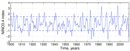
Abbildung 1: Temporal evolution of the NINO3.4 index that summarizes sea surface temperature (SST) anomalies in the region between 170$\degree$W–120$\degree$W and 5$\degree$S–5$\degree$N. The time series is centered and normalized, but the horizontal lines do not represent the standard deviations: instead, they have have ordinates 1.5 and -1; see also Fig. 3.

To simulate, understand and predict such complex phenomena one needs a full hierarchy of models, from “toy” via intermediate to fully coupled general circulation models (GCMs) (Neelin et al., 1998; Ghil and Robertson, 2000). We focus here on a “toy” model, which captures a qualitative, conceptual picture of ENSO dynamics that includes a surprisingly broad range of features. This approach allows one to gain a rather comprehensive understanding of the model’s, and maybe the phenomenon’s, underlying mechanisms and their interplay, at the cost of not capturing a full spatio-temporal picture of ENSO evolution.

We consider the following conceptual ingredients that play a determining role in the dynamics of the ENSO phenomenon: (i) the Bjerknes hypothesis, which suggests a positive feedback as a mechanism for the growth of an internal instability that could produce large positive anomalies of SSTs in the eastern Tropical Pacific (Bjerkness, 1969); (ii) delayed oceanic wave adjustments, realized in the form of eastward Kelvin and westward Rossby waves, that compensate for Bjerknes’s positive feedback (Suarez and Schopf, 1998); and (iii) seasonal forcing (Battisti, 1988; Chang et al., 1994, 1995; Jin et al., 1994, 1996; Tziperman et al., 1994, 1995; Ghil and Robertson, 2000). A more detailed discussion of these ingredients is given by Ghil et al. (2008b) and references therein.

The past 30 years of research have shown that ENSO dynamics is governed, by and large, by the interplay of the above nonlinear mechanisms and that their simplest version can be studied in periodically forced Boolean delay systems (Saunders and Ghil, 2001; Ghil et al., 2008a) and delay differential equations (DDE) (Suarez and Schopf, 1998; Battisti and Hirst, 1989; Tziperman et al., 1994). DDE models provide a convenient paradigm for explaining interannual ENSO variability and shed new light on its dynamical properties. So far, though, DDE model studies of ENSO have been limited to linear stability analysis of steady-state solutions, which are not typical in forced systems; case studies of particular trajectories; or one-dimensional (1-D) scenarios of transition to chaos, where one varies a single parameter while the others are kept fixed. A major obstacle for the complete bifurcation and sensitivity analysis of DDE models lies in the complex nature of DDEs, whose analytical and numerical treatment is considerably harder than that of their ordinary differential equation (ODE) counterparts.

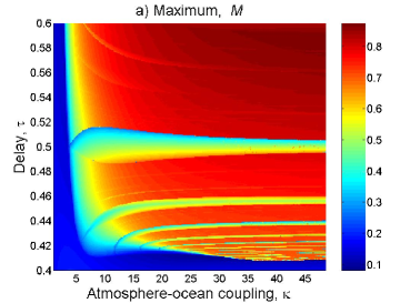
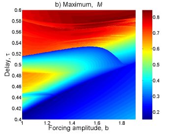
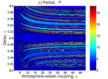
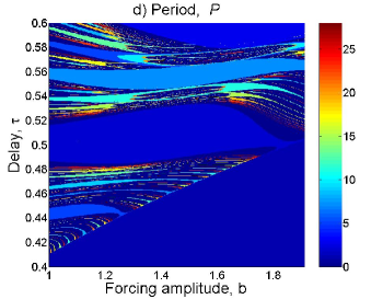
Abbildung 2: Maximum and period maps for a warm initial history, $\phi(t)\equiv 1$. ($a$) Maximum map, $M=M(\kappa,\,\tau)$ at $b=1$; ($b$) Maximum map, $M=M(b,\,\tau)$ at $\kappa=10$; ($c$) Period map, $P=P(\kappa,\,\tau)$ at $b=1$; ($d$) Period map, $P=P(b,\,\tau)$ at $\kappa=10$. Reproduced from Ghil et al. (2008b), with kind permission of Copernicus Publications on behalf of the European Geosciences Union (EGU).

0.2 Part 1 results and their physical interpretation

Ghil et al. (2008b) took several steps toward a comprehensive analysis, numerical as well as theoretical, of a DDE model relevant for ENSO phenomenology. In doing so, they also illustrated the complexity of the structures that arise in its phase-and-parameter space for even such a simple model of climate dynamics. Specifically, the authors formulated a highly idealized DDE model for ENSO variability and focused on the analysis of model solutions in a broad three-dimensional (3-D) domain of its physically relevant parameters. They showed that this model can reproduce many scenarios relevant to ENSO phenomenology, including prototypes of El Niño and La Niña events; spontaneous interdecadal oscillations; and intraseasonal activity reminiscent of Madden-Julian oscillations or westerly wind bursts.

This model was also able to provide a good justification for the observed quasi-biennial oscillation in Tropical Pacific SSTs and trade winds (Philander, 1990; Diaz and Markgraf, 1992; Jiang et al., 1995; Ghil et al., 2002), with the 2–3-year period arising naturally as the correct multiple of the sum of the basin transit times of Kelvin and Rossby waves. An important finding of Ghil et al. (2008b) was the existence of regions of stable and unstable solution behavior in the model’s parameter space; these regions have a complex and possibly fractal distribution of solution properties.

Figure 2 illustrates the model’s sensitive dependence on parameters in a region that corresponds roughly to actual ENSO dynamics. The figure shows the behavior of the global maximum $M$ and period $P$ of model solutions as a function of three parameters: the propagation period $\tau$ of oceanic waves across the Tropical Pacific, the atmosphere-ocean coupling strength $\kappa$, and the amplitude $b$ of the seasonal forcing; for aperiodic solutions we set $P=0$. Although the model is sensitive to each of these three parameters, sharp variations in $M$ and $P$ are mainly associated with changing the delay $\tau$, which is plotted on the ordinate in all four panels of the figure. In other words, the global maximum, in panels (a) and (b), as well as the period, in panels (c) and (d), may change more than twofold in response to a slight variation of $\tau$.

This sensitivity is an important qualitative conclusion since in reality the propagation times of Rossby and Kelvin waves are affected by numerous phenomena that are not related directly to ENSO dynamics. Moreover, the instabilities disappear and the dynamics of the system becomes purely periodic, with period one year, as soon as the atmosphere-ocean coupling $\kappa$ vanishes or the delay $\tau$ decreases below a critical value; see Figs. 2a, b. Finally, the boundary between the domains of stable and unstable model behavior is clearly visible in Fig. 2, in the lower-right part of panels (b) and (d).

The region below and to the right of this boundary contains simple period-one solutions that change smoothly with the values of model parameters. The region above and to the left is characterized by sensitive dependence on parameters. The range of parameters that corresponds to present-day ENSO dynamics lies on the border between the model’s stable and unstable regions. Hence, if the dynamical phenomena found in the model have any relation to reality, Tropical Pacific SSTs and other fields that are highly correlated with them, inside and outside the Tropics, can be expected to behave in an intrinsically unstable manner; they could, in particular, change quite drastically with global warming.

There are basically two approaches to ENSO dynamics (Neelin et al., 1994, 1998), both of which may be useful in extending the results of Part 1 above. The model considered here and in Ghil et al. (2008b) explains the complexities of ENSO dynamics by the interplay of two oscillators: an internal, highly nonlinear one, due to a delayed feedback, and a forced, seasonal one. Our model thus falls within the strongly nonlinear, deterministic approach.

An alternative approach attempts to explain several featureas of ENSO dynamics by the action of fast, “weathernoise on a linear or very weakly nonlinear “slowßystem, composed mainly on the upper ocean near the equator. Boulanger et al. (2004) and Lengaigne et al. (2004), among others, provide a comprehensive discussion of how weather noise could be responsible for the complex dynamics of ENSO, and, in particular, whether wind bursts trigger El Niño events. Saynisch et al. (2006) explore this possibility in a conceptual toy model. Ghil and Robertson (2000) already discussed the arguments about a “stochastic paradigm” for ENSO, with linear or only mildly nonlinear dynamics being affected decisively by weather noise, vs. a “deterministically chaotic paradigm,” with decisively nonlinear dynamics. Ghil et al. (2008c) have recently illustrated a way of combining these two paradigms to obtain richer and more complete insight into climate dynamics in general.

The present paper continues the study initiated in Part 1 and focuses (i) on the multiplicity of model solutions for the same parameter values; and (ii) on the behavior of local extrema in these solutions. In particular, we investigate the distribution in time of the model solutions’ maxima and minima; these extrema are directly connected to the strength and timing of the corresponding El Niño (warm) or La Niña (cold) events. The current analytic theory of DDEs does not allow one to easily answer many practically relevant questions about the behavior of even such apparently simple equations as our Eq. (1) below. The present study combines, therefore, general theoretical results about the existence and continuous dependence of solutions on parameters with extensive numerical investigations.

The rest of the paper is organized as follows. In Section 1, we summarize the model formulation from Part 1, recall basic theoretical results concerning this model’s solutions, and briefly review details of the numerical integration method. Section 2 reports on the phase locking of solutions to the periodic forcing, namely on the tendency for the solutions’ maxima and minima to each occur within a fixed, small interval of the seasonal cycle. Existence of multiple solutions and the attractor basins of the stable solutions are studied in Sect. 3. In Sect. 4 we investigate the behavior of the model’s local extrema, considered as a discrete dynamical system. A discussion of these results in Sect. 5 concludes the paper.

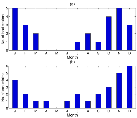
Abbildung 3: Histogram of temporal location of ($a$) warm and ($b$) cold events for the Niño–3.4 index. The event thresholds are shown by the dashed horizontal lines in Fig. 1. Notice the preferential occurrence of both warm and cold events during the boreal winter.

1 Model and numerical integration method

1.1 Model formulation and parameters

Following Part 1, we consider a nonlinear DDE with additive, periodic forcing,

$$h^{\prime}(t)=-a\,\tanh\left[\kappa\,h(t-\tau)\right]+b\,\cos(2\pi\,\omega\,t),$$ (1)

where $h^{\prime}(t)={{\mathrm{d}}h(t)}/{{\mathrm{d}}t}$, $t\geq 0$, and the parameters $a,\tau,\kappa,b,$ and $\omega$ are all real and positive. Equation (1) is a simplified one-delay version of the two-delay model considered by Tziperman et al. (1994); it includes two mechanisms essential for ENSO variability: a delayed, negative feedback via the function $\tanh(\kappa\,z)$, and periodic external forcing. As shown in Part 1, these two mechanisms suffice to generate very rich behavior that includes several important features of more detailed models and of observational data sets.

The function $h(t)$ in (1) represents the thermocline depth deviations from the annual mean in the eastern Tropical Pacific; accordingly, it can also be interpreted roughly as the regional SST, since a deeper thermocline corresponds to less upwelling of cold waters, and hence higher SST, and vice versa. The thermocline depth is affected by the wind-forced, eastward Kelvin and westward Rossby oceanic waves. The waves’ delayed effects are modeled by the function $\tanh\left[\kappa\,h(t-\tau)\right]$; the delay $\tau$ is due to the finite velocity of these waves and it corresponds roughly to their combined basin-transit time.

The particular form of the delayed nonlinearity plays an important role in the behavior of a DDE model. Munnich et al. (1991) provided a physical justification for the monotone, sigmoid nonlinearity we adopt here. The parameter $\kappa$, which is the linear slope of $\tanh(\kappa\,z)$ at the origin, reflects the strength of the atmosphere-ocean coupling. The forcing term represents the seasonal cycle in the trade winds, with the strongest winds occurring in boreal fall.

The DDE model (1) is fully determined by its five parameters: feedback delay $\tau$, atmosphere-ocean coupling strength $\kappa$, feedback amplitude $a$, forcing frequency $\omega$, and forcing amplitude $b$. By an appropriate rescaling of time $t$ and dependent variable $h$, we let $\omega=1$ and $a=1$. The remaining three parameters — $\tau$, $\kappa$, and $b$ — may vary, reflecting different physical conditions of ENSO evolution. We consider here the same parameter ranges as in Part 1 of this study: $0\leq\tau\leq 2$ yr, $0<\kappa<\infty$, $0\leq b<\infty$.

To completely specify model (1) we need to prescribe some initial “history,” i.e. the behavior of $h(t)$ on the interval $[-\tau,\,0)$, cf. Hale (1977). In the numerical experiments of Sect. 2 below we assume, as in Part 1, that $h(t)\equiv 1$, $-\tau\leq t<0$, i.e. we start with a warm year. But in Sect. 3 we turn to a systematic exploration of the effect of the initial histories on the number and stability of solutions.

Abbildung 4: Seasonal phase locking of local extrema for model trajectories: (a–c) with period $P=1$; (d–f) with period $P=7$; and (g–i) aperiodic. The model solutions in panels ($a,d,g$) are shown in the stationary regime, after a sufficiently long transient, and the time axis is shifted so as to start from $t=0$. The parameter values for these solutions are ($a$) $\tau=0.5$, $\kappa=11$, $b=2$; ($d$) $\tau=0.56$, $\kappa=11$, $b=1.4$; and ($g$) $\tau=0.47$, $\kappa=10$, $b=1.0$. The scatterplots of the points $(h(t_{i}),h(t_{i}+1))$ in panels ($b,e,h$) use the values $i=0,1,\dots,500$, which correspond to $t_{0}=2500$ and the parameter settings in panels ($a,d,g$), respectively. The phase locking is illustrated in panels ($c,f,i$), which give the $h$-value of the local extrema — maxima shown as red filled circles and minima as blue squares — as a function of their position within the seasonal cycle, $\varphi=t({\rm mod}\leavevmode\nobreak\ 1)$.

1.2 Main theoretical result

Consider the Banach space $X=C([-\tau,0),\mathbb{R})$ of continuous functions $h\,:\,[-\tau,0)\to\mathbb{R}$ and define the norm for $h\in X$ as

$$\parallel h\parallel=\sup\left\{|h(t)|,\leavevmode\nobreak\ t\in[-\tau,0)\right\},$$

where $|\cdot|$ denotes the absolute value in $\mathbb{R}$ (Hale, 1977; Nussbaum, 1998). For convenience, we reformulate the DDE initial-value problem (IVP) in its rescaled form:

$$h^{\prime}(t) = -\tanh\left[\kappa\,h(t-\tau)\right]+b\,\cos(2\pi\,t),\leavevmode\nobreak\ t\geq 0,$$ (2)

$$\quad h(t) = \phi(t)\leavevmode\nobreak\ \leavevmode\nobreak\ {\rm for\leavevmode\nobreak\ }\leavevmode\nobreak\ t\in[-\tau,\,0),\quad\phi(t)\in X.$$ (3)

Ghil et al. (2008b) proved the following result, which follows from Hale and Verduyn Lunel (1993) and references therein.

Proposition 1

(Existence, uniqueness, continuous dependence) For any fixed positive triplet $(\tau,\,\kappa,\,b)$, the IVP (2)-(3) has a unique solution $h(t)$ on $[0,\,\infty)$. This solution depends continuously on the initial data $\phi(t)$, delay $\tau$ and the right-hand side of (2), considered as a continuous map $f\,:\,[0,T)\times X\to\mathbb{R}$, for any finite $T$.

From Proposition 1 it follows, in particular, that the system (2)-(3) has a unique solution for all time, which depends continuously on the model parameters $(\tau,\,\kappa,\,b)$ for any finite time. This result implies that any discontinuity in the solution profile, as a function of the model parameters, indicates the existence of an unstable solution that separates the attractor basins of two stable solutions. Our numerical experiments suggest, furthermore, that all stable solutions of (2)-(3) are bounded and have an infinite number of zeros.

1.3 Numerical integration

The results in this Part 2 of our study are based on numerical integration of the DDE (2)-(3). We emphasize that there are important differences between the numerical integration of DDEs and ODEs, and that these differences require developing special software; often the problem-specific modification of such software also becomes necessary. We used here the Fortran 90/95 DDE solver dde_solver of Shampine and Thompson (2006), available at http://www.radford.edu/~thompson/ffddes/. Technical details of dde_solver, as well as a brief overview of other available DDE solvers, are given in Appendix C of Part 1.

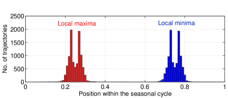
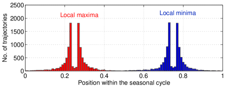
Abbildung 5: Seasonal phase locking of local extrema: cumulative results. Histogram of the phase $\varphi$ of the local maxima (red bars) and minima (blue bars) of model solutions with $\kappa=2.0$ (top panel) and $\kappa=11.0$ (bottom panel). Each panel uses 10 000 individual solutions with parameters $0<\tau\leq 2$ and $0<b\leq 10$; see also Fig. 6.

2 Seasonal phase locking of extrema

A distinctive feature of the extreme ENSO phases — i.e., of the El Niño and La Niña events — is their occurrence during a boreal winter. This phenomenon is illustrated in Fig. 3, which shows the histograms of the monthly positions of unusually warm and unusually cold events, based on the Niño–3.4 index of Fig. 1. In our classification, El Niños (see panel $a$) are those for which NINO3.4 $>1.5$, while La Niñas (see panel $b$) have NINO3.4 $<-1$. This asymmetry in the classification is due to the fact that extreme warm events are more intense but fewer in number than the extreme cold events (Hoerling et al., 1997; Burgers and Stephenson, 1999; Sardeshmukh et al., 2000; Kondrashov et al., 2005). Clearly, the extreme events, both warm and cold, tend to occur during boreal winter.

In discussing extrema, we distinguish between local and global ones. Recall that for a function $h(t)$ specified on the interval $[t_{1},t_{2}]$, its global maximum (minimum) is defined as the point $t$ such that $h(t)$ is above (below) all the other values on that interval: $h(t)\geq h(s)$, respectively $h(t)\leq h(s)$, for all $s\in[t_{1},t_{2}]$. A local maximum (minimum) is a point $t$ such that the corresponding value $h(t)$ is above (below) all the values in a vicinity of $t$; for a sufficiently smooth function, the latter definitions are equivalent to

$${\rm(i)}\quad h^{\prime}(t)=0;\quad{\rm and}\quad{\rm(ii)}\quad h^{\prime\prime}(t)<0\quad{\rm or}\quad h^{\prime\prime}(t)>0,$$

where $h^{\prime\prime}=(h^{\prime})^{\prime}$ is the second derivative of $h(t)$.

In this paper, we work with numerical solutions of the DDE problem (2)-(3) that are available only on a finite time interval $[0,t_{f}]$; in addition, we eliminate the initial transient interval $[0,t_{0})$. We thus consider the global and local extrema of our solutions only on the interval $[t_{0},t_{f}]$. The global extrema thus defined might differ in certain cases from their counterparts on the interval $[0,\infty)$, for which our DDE is formally defined. The difference will only be noticeable for very–long-periodic, highly fluctuating solutions that are relatively rare in our model. Hence, the reduced definitions of the global and local extrema do not affect the main conclusions of our analysis.

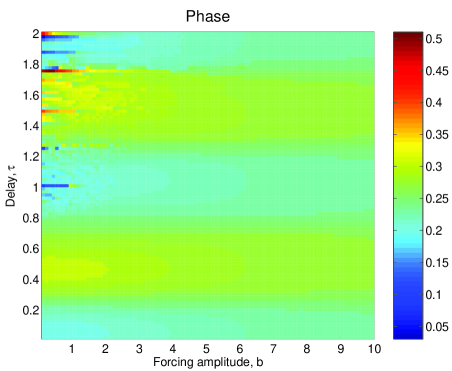
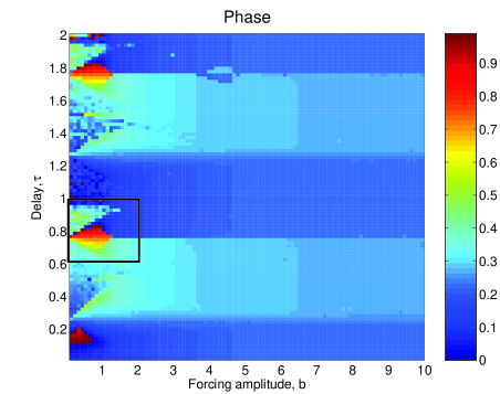
Abbildung 6: Seasonal phase locking of global extrema: parameter dependence. The plots show the phase $\varphi$ of the global maxima of solutions of Eq.  (2) for $\kappa=2.0$ (top panel) and $\kappa=11.0$ (bottom panel); same number of solutions and parameter range as in Fig. 5. The rectangle in the bottom panel highlights the region blown up in Fig. 7.

In this section, we study the phase $\varphi$ of the local maxima and minima of the model solutions that obey (2)-(3). The main result, as we shall see, is that the model’s extrema occur exclusively within a particular season.

We start with several examples that illustrate the analysis in the rest of the section. Figure 4$a$ shows a piece of model solution $h(t)$ for $\tau=0.5$, $\kappa=11$, and $b=2$. This solution has period $P=1$, as illustrated in panel ($b$), which shows the scatterplot of the pairs $(h(t_{i}),h(t_{i}+1))$ for $i=0,1,\dots$ and $t_{i+1}=t_{i}+1$. Given the 1-periodic character of the solution, all the points $(h(t_{i}),h(t_{i}+1))$ coincide. The choice of the starting point $t_{0}$ will only affect the position of a single point in the panel (not shown).

For each time epoch $t$ we define its position $\varphi$ within the seasonal cycle as $\varphi=t({\rm mod}\leavevmode\nobreak\ 1)$; the origin of the seasonal cycle in the forcing is taken in October, when the trade winds are strongest. Panel ($c$) shows the values of the local maxima (filled circles) and minima (squares) of $h(t)$ as a function of their position $\varphi$ within the seasonal cycle. The six other panels in Fig. 4 show the results of a similar analysis for a solution with period $P=7$ (panels $d-f$) and an aperiodic one (panels $g-i$).

In all the examples of Fig. 4, most of the local maxima are located within the first half of the annual cycle, i.e. in boreal winter, while the local minima lie within the second half, i.e. in boreal summer. Moreover, the global maximum, as well as local maxima with large amplitudes, are always located within the $\varphi$-interval $(0.15,0.4)$, while the global minimum, as well as large-amplitude local minima, are always located within the interval $(0.7,0.95)$. We found this characteristic property of the model to hold for most of its solutions.

To verify this model property, we analyzed the positions of the local extrema for a large number of individual solutions of Eq. (2) within the parameter region $(0<\tau\leq 2,0<b\leq 10)$ and at several values of $\kappa$. The representative results are summarized in Figs. 5 and 6, where we used 10 000 individual solutions for each value of $\kappa$. Figure 5 shows histograms of positions of the local extrema within the seasonal cycle, while Fig. 6 plots the position of the global maximum as a function of the model parameters $\tau$ and $b$.

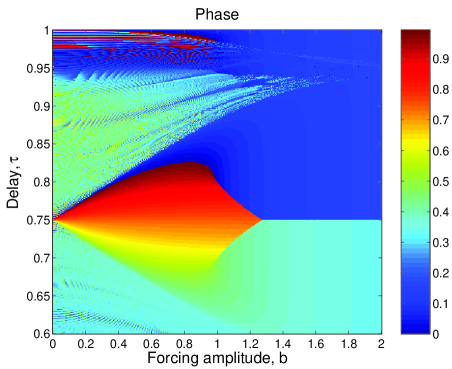
Abbildung 7: Reversal in the phase locking of the maxima. The plot shows the seasonal cycle position $\varphi$ of the global maximum for 250 000 solutions of Eq.  (2), for $\kappa=11.0$; it represents a blow-up of the region marked by a rectangle in the lower panel of Fig. 6.

The phase locking of the extrema to the seasonal cycle is present for most combinations of the physically relevant model parameters. Moreover, the local maxima tend to occur, depending on the value of $\tau$, at either $\varphi=0.23$ or $\varphi=0.27$, while the local minima occur at $\varphi=0.73$ or $\varphi=0.77$. We notice that the cosine-shaped seasonal forcing vanishes at $\varphi=0.25$ and $\varphi=0.75$; hence the local maxima occur in the vicinity of zero forcing when the latter decreases, and the local mimina occur in the vicinity of zero forcing when the latter increases. The offset in the position of the extrema from the point where the external forcing vanishes seems to be independent of the model parameters.

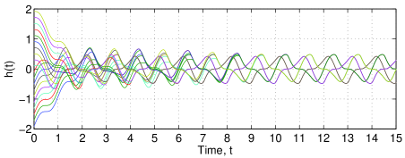
Abbildung 8: Multiple stable solutions. Twenty trajectories that correspond to different initial histories $\phi(t)\equiv\phi_{0}$ collapse, after a transient, onto four stable solutions. Two of these solutions are distinct, and the other two can be obtained from the latter by a time shift. Model parameters are $\tau=0.5$, $\kappa=10$, and $b=1$; see also Fig. 9.

As the atmosphere-ocean coupling parameter $\kappa$ increases, yet another type of sensitive dependence on parameters sets in. Namely at low values of the external forcing, $b<1.5$, “reversals” in the location of the local extrema do occur, with maxima suddenly jumping to boreal summer and minima to boreal winter. In Fig. 7, we zoom into one such reversal region, marked by a rectangle in Fig. 6. The dark and light blue colors that occupy most of the region indicate that the global maximum of a model solution occurs in the first half of the annual cycle, while the red-to-yellow colors that appear around $\tau=0.75$ indicate that, within this “island,the global maximum jumps to the annual cycle’s second half.

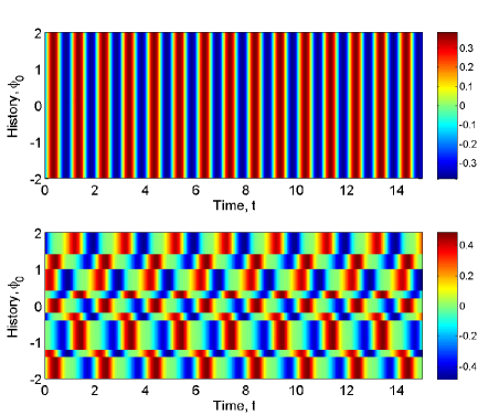
Abbildung 9: Solution profiles for multiple constant histories $\phi(t)=\phi_{0}$. The top panel corresponds to point $A=(\tau=0.4,\kappa=11,b=2)$ in parameter space, where there exists a unique stable solution. The bottom panel corresponds to $B=(\tau=0.5,\kappa=10,b=1)$, the same point as in Fig. 8; here there exist two stable solutions and their attractor basins are bounded by horizontal discontinuity lines in the solution profile. The solutions are shown after a sufficiently long transient, and the origin of the time is shifted to start from zero; color bars indicate solution values, here as well as in Fig. 10.

3 Multiple solutions, stable and unstable

The analysis in the previous section was carried out, as in Part 1, for the model (2)-(3) with a fixed initial history, $\phi(t)\equiv 1$. In this section, we study the model’s solutions for distinct, yet still constant histories $\phi(t)\equiv\phi_{0}$.

Naturally, different initial history values $\phi_{0}$ may result in different model solutions. This is illustrated in Fig. 8 for the parameter values $\tau=0.5$, $\kappa=10$, and $b=1$. To produce this figure we used 20 distinct initial histories, with constant values that are uniformly distributed between $\phi_{0}=-2$ and $\phi_{0}=2$; hence, at time $t=0$ there exist 20 distinct solutions. As time passes, those solutions are attracted by a smaller number of stable solutions so that, by $t=15$, there are only four distinct solutions left, all of which have period $P=2$. We notice furthermore that two of the remaining four solutions can be obtained by shifting the other two by one unit of time.

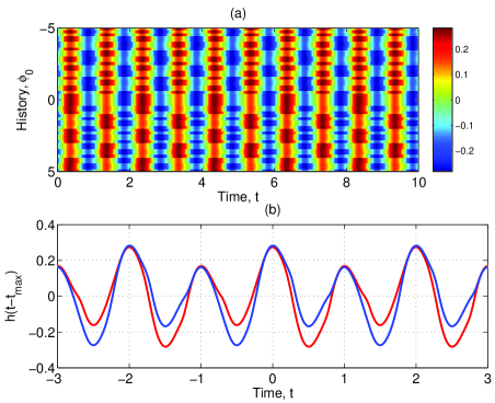
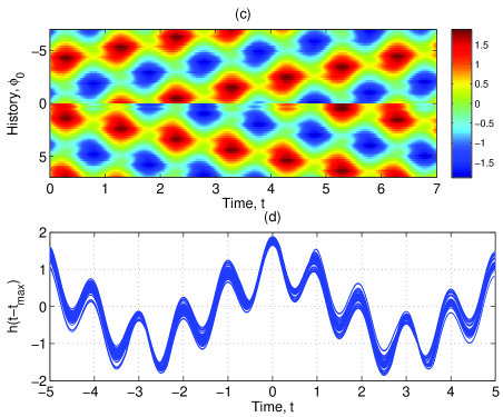
Abbildung 10: Multiple stable solutions. Solution profile for ($a,c$) different initial histories $\phi(t)\equiv\phi_{0}$, and ($b,d$) the corresponding distinct solutions. For visual convenience, the trajectories are shifted to have their global maxima at $t=0$. Panels ($a,b$): model behavior at point $C=(\tau=0.5,\kappa=11,b=1.7842)$, where there exist 2 distinct solutions; and panels ($c,d$): model behavior at point $D=(\tau=1.4579,\kappa=11,b=4)$, where there exist 61 distinct solutions.

In general, it is readily seen that — if the system (2)-(3) has solution $x(t)$ — then $x(t+k)$ with any integer $k$ is also a solution. Hence, if $x(t)$ is a solution with integer period $P=k$, then there are $k-1$ other solutions obtained from $x(t)$ by an integer time shift. We will focus on solutions that cannot be obtained from each other by such a shift. Thus, we call two solutions $x(t)$ and $y(t)$ distinct if $x(t)\not\equiv y(t+k)$ for any positive integer $k\neq P$.

Next we concentrate on the attractor basins of the model’s stable solutions. Figure 9 shows the model’s solution profiles, after a suitable transient, for $-10\leq\phi_{0}\leq 10$, at two points in the model’s parameter space: point $A=(\tau=0.4,\kappa=1,b=2)$ in the top panel, and point $B=(\tau=0.5,\kappa=10,b=1)$ in the bottom panel. Model behavior at point $B$ was illustrated in Fig. 8. At point $A$ the model has a unique stable solution that attracts all transient solutions as time evolves, so that the solution profile becomes constant along any vertical line, i.e. at any $t=t_{0}$ in this type of figure.

The model has two distinct stable solutions at point $B$: the boundary between their attractor basins, as plotted on the real line of initial-history values $\phi_{0}$, corresponds to points of discontinuity in the solution profiles. These points line up into straight horizontal lines in Fig. 9: one can see 8 horizontal lines of discontinuity in the solution profiles and there would thus appear to be 9 attractor basins. These basins correspond, however, as shown in Fig. 8, to only two stable solutions that are distinct from each other.

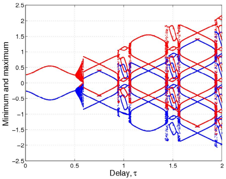
Abbildung 11: Local maxima (red) and minima (blue) of model solutions as a function of delay $\tau$; the other parameter values are fixed at $\kappa=11$ and $b=2$. Notice the aperiodic regimes between periodic windows of gradually increasing period.

Recall from Sect. 1.2 that our solutions lie in the infinite-dimensional Banach space $X=C([-\tau,0),\mathbb{R})$, and that the solutions with constant initial histories do not span this space. By using such a particularly simple type of initial histories, we are merely exploring a 1-D manifold of solutions, parametrized by the scalar $\phi_{0}$, in the full space $X$. The intersection of the boundary between the attractor basins of the two stable solutions with this 1-D manifold gives the 8 lines of discontinuity seen in the bottom panel of Fig. 9.

Proposition 1 also implies that a discontinuity in the solution profile at $\phi_{0}$ suggests that there exists an unstable solution starting from $\phi(t)\equiv\phi_{0}$. Hence, the boundary that separates the two attractor basins from each other is formed by unstable model solutions. This boundary is a manifold of codimension one in $X$, and Figure 9 reveals merely the intersection of this manifold with the 1-D manifold of solutions that have constant initial histories. The presence of 8 such intersections suggests, in turn, that the boundary between the two attractor basins is a highly curved, but still smooth manifold. It is known for finite-dimensional problems that such boundaries can become quite complex and possibly fractal (Grebogi et al., 1987).

Figure 10 shows two slightly more complex situations along the same lines, namely one with still only two distinct solutions, having both period $P=2$, but a more intricate pattern of solution profiles (panels $a,b$), and one with 61 distinct solutions, having all $P=10$ (panels $c,d$). For visual convenience we shift all the solutions so that their global maxima occur at $t=0$.

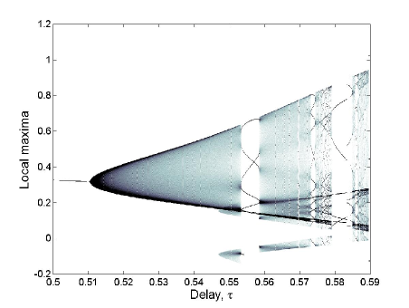
Abbildung 12: Distribution of local maxima as a function of delay $\tau$ within the interval $0.5<\tau<0.59$; the other parameters are as in Fig. 11.

4 Dynamics of local extrema

We focus here on the dynamics of the local extrema in the model solutions. For each solution $h(t)$ we consider the sequence of its local extrema $\{e_{i}\}:=\{h(t_{i})$, $i=1,2,\dots\}$, where $h^{\prime}(t_{i})=0$. The local maxima $\{M_{i}$, $i=1,2,\dots\}$ are characterized by the additional condition that $h^{\prime\prime}(t_{i})<0$, while at the local minima $\{m_{i}$, $i=1,2,\dots\}$ one has $h^{\prime\prime}(t_{i})>0$.

Figure 11 shows the position of the local extrema as a function of delay $0<\tau<2$ for fixed $\kappa=11$ and $b=2$. The figure illustrates convincingly the increase in complexity of model solutions as the delay $\tau$ increases. For small delay values, $0<\tau<0.5$, each solution is a periodic sine-like wave with period $P=1$, which contains a single maximum and a single mimimum within each cycle.

Within the interval $0.6<\tau<0.8$ the solutions become more complex: the solution period here is $P=3$, and each cycle has three local maxima and three local minima. In general, the time elapsed between a local maximum and the next is an integer number; this effect is caused by the seasonal forcing, and the same is true for local minima. Often, the recurrence interval for extrema of the same kind is just unity and the number of local maxima (or minima) coincides with the period $P$ of a given solution.

The period in Fig. 11 increases by jumps of 2, from $P=1$ to $P=3$ and so on, as $P=2k+1$. The transitions from one odd-periodic dynamics to the next are associated each time with a region of aperiodic behavior; e.g. the one from $P=1$ to $P=3$ occurs in the interval $0.51<\tau<0.59$. Thus, as $\tau$ increases, the number of local extrema becomes larger and each increase in the number of extrema is preceded by a region of aperiodic, presumably chaotic behavior.

Figure 12 zooms in on the distribution of local maxima within the first aperiodic region of Fig. 11, namely $0.51<\tau<0.59$. In this region, the $\tau$-intervals of aperiodic behavior alternate with shorter periodic windows: in the former the local maxima are distributed continuously within an interval, while in the latter several distinct local maxima occur within a comparable range of values. This distribution of the maxima resembles the behavior of chaotic dynamical systems in discrete time — e.g., period doubling for smooth maps (Feigenbaum, 1978; Kadanoff, 1983) — and suggests that the model’s aperiodic dynamics is in fact chaotic. An even richer behavior — with multiple, overlapping cascades — seems to emerge for $0.545<\tau$.

5 Concluding remarks

In the present paper we continued our study of a periodically forced delay differential equation (DDE) introduced by Ghil et al. (2008b); the DDE (1) serves as a toy model for ENSO variability. We studied the model solutions numerically in a broad 3-D domain of physically relevant parameters: oceanic wave delay $\tau$, ocean-atmosphere coupling strength $\kappa$, and seasonal forcing amplitude $b$. In this Part 2 of our investigation, we focussed on multiple model solutions as a function of initial histories, and on the dynamics of local extrema.

We found that the system is characterized by phase locking of the solutions’ local extrema to the seasonal cycle (Figs. 4 and  5): solution maxima — i.e., warm events (El Niños) — tend to occur in boreal winter, while local minima — i.e., cold events (La Niñas) — tend to occur in boreal summer. The former model feature is realistic, since observed warm events do occur by-and-large in boreal winter; in fact, this property is one of the main features of the observed El Niño events, having even given rise to the name of the phenomenon (Philander, 1990; Glantz et al., 1991; Diaz and Markgraf, 1992).

The phase locking of cold events in the model to boreal summer is not realistic, since La Niñas also tend to occur in boreal winter, rather than in phase opposition to the warm ones; see again Fig. 3. It is not clear at this point which one of the lacking features of our DDE model gives rise to this unrealistic phase opposition; it might be the lack of a positive feedback mechanism, present with a separate, distinct delay in the Tziperman et al. (1994) model. On the other hand, even GCMs with many more detailed features may have their warm events in entirely the wrong season; see Ghil and Robertson (2000) for a review.

At the same time, for small-to-intermediate seasonal forcing $b$, the position of the global maxima and minima depends sensitively on other parameter values: it may exhibit significant jumps in response to vanishingly small changes in the parameter values (Fig. 6). In particular, an interesting phenomenon of “phase reversalöf the global extrema may occur, cf. Fig. 7.

We explored a 1-D manifold of solutions for a set of given, prescribed points $P=(\tau,\kappa,b)$ in the model’s parameter space. Such a manifold was generated, for each $P$, by solutions with constant initial histories $\phi(t)\equiv\phi_{0}$.

We found multiple solutions coexisting for physically relevant values of the model parameters; see Figs. 8–10. Some of these solutions are generated by shifting a single solution in time, using integer multiples of the period of the forcing, taken here to be unity. We have often found a set of $k$ solutions so obtained from a single solution of period $P=k$.

Typically, each stable solution has a bounded, but infinite-dimensional attractor basin in the solution space $X$ described in Sect. 1.2. This attractor basin is separated from that of another stable solution by a manifold of codimension one, which is generated by unstable solutions (see Proposition 1 and the following remarks). The intersections of such a manifold with the 1-D manifold of solutions explored herein appear as the straight horizontal lines in the solution-profile panels of Figs. 9 and 10.

In Part 1, we found that the solution period generally increases with the oceanic wave delay $\tau$. Figures 11 and 12 here provide much more detailed information: the period $P$ of model solutions increases in discrete jumps, like $\{P=2k+1,k=0,1,2,\dots\,\}$, separated by narrow, apparently chaotic “windowsïn $\tau$. This increase in $P$ is associated with the increase of the number of distinct local extrema, all of which tend to occur at the same position within the seasonal cycle. The distribution of the maxima in Fig. 12 resembles in fact the behavior of chaotic dynamical systems in discrete time (Feigenbaum, 1978; Kadanoff, 1983) and suggests that the model’s aperiodic dynamics is in fact chaotic.

It is quite interesting that, for plausible values of the delay $\tau$, the periods lie roughly between 2 and 7 years, a range that is commonly associated with the recurrence of relatively strong warm events (Philander, 1990; Glantz et al., 1991; Diaz and Markgraf, 1992; Neelin et al., 1998). The sensitive dependence of the period on the model’s external parameters $(\tau,\kappa,b)$ is consistent with the irregularity of occurrence of strong El Niños, and can help explain the difficulty in predicting them (Latif et al., 1994; Ghil and Jiang, 1998).

Acknowledgements We are grateful to our colleagues M. D. Chekroun, J. C. McWilliams, J. D. Neelin and E. Simonnet for many useful discussions; MDC in particular suggested the search for multiple solutions, and JDN provided information on the seasonal cycle in the surface winds. This study was supported by DOE Grants DE-FG02-07ER64439 and DE-FG02-07ER64440 from the Climate Change Prediction Program, and by the European Commission’s No. 12975 (NEST) project “Extreme Events: Causes and Consequences (E2-C2).”