On-shell Recursion in String Theory

Abstract:

We prove that all open string theory disc amplitudes in a flat background obey Britto-Cachazo-Feng-Witten (BCFW) on-shell recursion relations, up to a possible reality condition on a kinematic invariant. Arguments that the same holds for tree level closed string amplitudes are given as well. Non-adjacent BCFW-shifts are related to adjacent shifts through monodromy relations for which we provide a novel CFT based derivation. All possible recursion relations are related by old-fashioned string duality. The field theory limit of the analysis for amplitudes involving gluons is explicitly shown to be smooth for both the bosonic string as well as the superstring. In addition to a proof a less rigorous but more powerful argument based on the underlying CFT is presented which suggests that the technique may extend to a much more general setting in string theory. This is illustrated by a discussion of the open string in a constant B-field background and the closed string on the level of the sphere.

1 Introduction

Recent years have seen many new techniques and insights for the calculation of scattering amplitudes within field theory inspired by Witten’s twistor string proposal [1]. Since field theory arises as the low energy limit of ordinary string theory in a flat background, a natural question is to what extent these advances for fields can be carried over to strings in this setting. This is especially important as much useful information about the string theory can be obtained directly from the amplitudes and vice-versa. In this context it is noteworthy that much of the recent field theory progress is based on the same ‘analytic S-matrix’ type approach which originally led to the birth of string theory [2]. Besides aiming for direct benefits in field theory applications there is an intrinsic interest in understanding string theory better. Although in this article the focus will be mostly on flat backgrounds, a longer term goal of our program is to understand string theory in curved backgrounds as this relates directly to strong coupling field theory through the AdS/CFT correspondence [3].

In this article the Britto-Cachazo-Feng-Witten (BCFW) on-shell recursion relations [4, 5] are studied in the context of string theory. In field theory these useful relations relate tree level amplitudes to a sum over amplitudes with a smaller number of particles, evaluated at complex values of the momenta. The elementary and elegant derivation of the relations [5] involves a complex momentum shift on two particles. Crucially, an absence of certain residues at infinite momentum shifts needs to be shown to make the relations work. Residues at infinite complex momentum are at the least by hand waving related to the UV behavior of the theory under study. This reasoning can be made more precise in field theory [6]. Absence of residues at infinity has been proven in (super)Yang-Mills and Einstein (super)gravity in any dimension from four onwards, see [7], [8] and references therein. Of course, string theory has excellent UV behavior and a natural question is whether string theory amplitudes also obey similar on-shell recursion relations.

The string version of on-shell recursion relations was first investigated by K. Larsen, M. Vonk and two of the present authors in [9], where these relations were shown to hold for all four-particle amplitudes in both the open and the closed string in a flat background and for a certain five-particle amplitude in four dimensions. Already there it was striking how natural on-shell recursion appears in string theory. However, the analysis of [9] was based on fully integrated forms of the amplitude. As these are unknown for larger ($>\sim 5$) numbers of external particles, the approach of [9] is unsuitable for a general analysis. The aim of this paper is to change this situation.

An outline and summary of the main results is as follows. We start in Section 2 by examining adjacent shifts in open string amplitudes based on the integral expressions, up to the determination of a certain kinematic constraint. This constraint is determined explicitly for amplitudes with shifted gluon legs in both the bosonic string as well as the superstring. Non-adjacent shifts are treated in Section 3, based on the monodromy relations for string theory amplitudes first presented in [15] and recently discussed in [16] and [17]. It is shown how these monodromy relations follow directly from the underlying CFT which may be of independent interest. The outlines of a completely CFT-based derivation of the adjacent shift behavior of any amplitude is presented in Section 4. This powerful technique will be applied in two sample cases in Section 5. One is a generalization of our results to open string amplitudes in constant B-field backgrounds. The other is a CFT analysis of the large shift behavior for the closed string. An independent argument based on the Kawai-Lewellen-Tye (KLT) relations [18] is also included there. A discussion, conclusions and some speculations round off the main presentation in Section 6. In Appendix A shifts of the four point gluon amplitude in the bosonic string and the superstring are presented as a worked-out example. Appendix B contains a proof of a technical point. Finally, in Appendix C naive application of a three particle shift originally used to derive the CSW rules in field theory is shown to lead to inconsistent results for four particle superstring amplitudes.

Note added in proof: While this paper was being readied for publication [19] appeared which has a sizeable overlap with the techniques and results presented here, especially in section 4.

2 Recursion relations for the disc: adjacent shifts

2.1 Lightning review of on-shell recursion

The key observation for deriving the on-shell recursion relations is that any tree level scattering amplitude can easily be turned into a rational function of a single complex variable by deforming the momenta [5], requiring that these deformed momenta remain on-shell and obey momentum conservation. The simplest example of this is to take two particles $i$ and $j$ and shift their momenta by a vector $q_{\mu}$

$$p^{\mu}_{i} \rightarrow\hat{p}^{\mu}_{i}=p_{i}^{\mu}+zq^{\mu}\ ,$$

$$p^{\mu}_{j} \rightarrow\hat{p}^{\mu}_{j}=p_{j}^{\mu}-zq^{\mu}\ ,$$ (1)

which preserves momentum conservation. For an example of a more complicated shift see appendix C. For two particle shifts linear in $z$ as in eq. (1), the on-shell constraint is satisfied iff the vector $q$ obeys

$$p^{\mu}_{i}q_{\mu}=p^{\mu}_{j}q_{\mu}=q^{\mu}q_{\mu}=0\ .$$ (2)

These equations do not have a solution for real $q_{\mu}$, but do for complex momenta, as can easily be verified by going to the common lightcone frame.

After the shift any $n$-point amplitude $A_{n}$ becomes a function of a complex variable $A_{n}(z)$, where the amplitude of interest is of course $A_{n}(z=0)$. This can be obtained by an elementary contour integration around a contour which only encompasses the pole at $z=0$,

$$A_{n}(0)=\oint_{z=0}\frac{A_{n}(z)}{z}dz\ .$$ (3)

If the contour is now pulled to the other side of the Riemann sphere one encounters various poles at finite values of $z$ and a possible residue at infinity,

$$A_{n}(0)=\oint_{z=0}\frac{A_{n}(z)}{z}dz=-\left\{\sum\mathrm{Res}_{z=\textrm{finite}}+\mathrm{Res}_{z=\infty}\right\}\ .$$ (4)

The poles at finite values of $z$ correspond to the exchange of physical particles. By tree level unitarity, the residues at these poles must be the product of two tree level amplitudes with each one leg containing the particle being exchanged, summed over all particles at this particular mass level. The residue at infinity does not have a similar physical interpretation. If therefore this residue vanishes then all terms on the right hand side of (4) are known and consist of lower point amplitudes. Therefore in this case a recursion relation is obtained between amplitudes

$$A_{n}(1,2,3\ldots,n)=\sum_{r,h(r)}\sum_{k=2}^{n-2}\frac{A_{k+1}(1,2,\ldots,\hat{i},\ldots,k,\hat{P}_{r})A_{n-k+1}(\hat{P}_{r},k+1,\ldots,\hat{j},\ldots,n)}{\left(p_{1}+p_{2}+\ldots+p_{k}\right)^{2}+m_{r}^{2}}\ ,$$ (5)

where the first sum is over all different mass levels $r$ and over all polarization states at that level, denoted $h(r)$. The momentum $\hat{P}_{r}$ for the ‘extra’ particle and its anti-particle in the amplitude is such that the particle is on-shell. This condition determines the numerical value of $z$. The second sum over $k$ is over all the different ways in which the amplitude can be factorized with the shifted legs on the different amplitudes in the residues. Note that for every different term in the $k$ sum the numerical value of $z$ entering the residue is different.

The challenge in deriving this relation is proof of absence of the residue at infinity. This proof will be provided for all open string theory amplitudes in a flat background in this paper, subject to a kinematic constraint. As the derivation of the BCFW recursion relation involves a limit, the field theory limit of the resulting equations has to be treated with care [9] to avoid ‘order of limits’ problems. Note that any symmetry of the three-point amplitude will imply through the recursion relations a corresponding symmetry of $n$-point amplitudes.

Dimensionality of space-time

Our analysis of on-shell recursion in string theory will hold in principle for any dimensionality of the target space-time. However, in the recursion relations one has to sum over all particles appearing in the theory. Hence in dimensions above the usual critical dimension of the string theory of interest negative norm states have to be included for instance. In dimensions below the critical dimension, one can use a dimensional reduction argument to reduce the amplitude from the critical dimension to fields in the dimension one is interested in. Although it would certainly be interesting to study non-critical string amplitudes this is beyond the scope of the present paper.

Relation to factorization formulae

The recursion relation in eq. (5) has a passing resemblance to factorization formulas as studied in the beginning days of string theory. See for example equation $90$ in [20], or chapter 7 of [21]. One can write any string amplitude in terms of so-called Feynman-like diagrams. Diagrammatically, this corresponds to molding the string world-sheet into the rough shape of a particular Feynman graph with a certain manifest singularity structure. In formulas this reads,

$$A=\langle k_{1}|V_{2}DV_{3}\ldots V_{n-1}|k_{n}\rangle\ ,$$ (6)

where $D$ is the string theory propagator $\frac{1}{L_{0}-1}$. Now one can insert a complete set of states next to one propagator, say the first one,

$$A=\langle k_{1}|V_{2}\left(\sum_{\lambda}|\lambda,P\rangle\langle P,\lambda|\right)\left(\frac{1}{L_{0}-1}\right)\left(\sum_{\lambda^{\prime}}|\lambda^{\prime},P\rangle\langle P,\lambda^{\prime}|\right)V_{3}\ldots V_{n-1}|k_{n}\rangle\ ,$$ (7)

where

$$P=k_{1}+k_{2}\ .$$ (8)

This expression has manifest poles as a function of $P$: these are such that the states are annihilated by $L_{0}-1$. Therefore, precisely at these poles the amplitude factorizes. This is one way to see that string theory amplitudes have the poles required by tree level unitarity. Away from the poles however one has to sum over all states in the Hilbert space of the harmonic oscillators of the string which include unphysical modes. Demonstrating that these modes decouple in physical amplitudes (i.e. in the residue at the pole) was the main objective of the beginning days of string theory. In general however, the momentum in the channel for which the poles are displayed is not on-shell. Hence eq. (7) certainly does not express an amplitude in terms of lower point amplitudes, except in the limit where the sum of the momenta on the left hand side squared approaches its pole value. In contrast, (5) expresses the amplitude for generic momenta as a sum over a subset of the poles of the amplitude, with the residue modified by the shifted momenta.

One can point to more differences between factorization formulas and on-shell recursion. For instance, the formula in eq. (5) is a sum over all the channels for which the shifted momenta appear on the left and right hand side, whereas eq. (7) above displays poles in one channel only. Moreover, eq. (5) involves shifted momenta. That implies for one that the numerical values of the momenta on the amplitudes for both the shifted legs as well as the intermediate channel are different from the above factorization formulae and are different for every different channel in the sum.

2.2 Veneziano revisited

To get an idea for how to proceed, it is instructive to revisit the (ordered) Veneziano amplitude [2] for the scattering of four tachyons in open bosonic string theory,

$$A(s,t)=\frac{\Gamma({\alpha^{\prime}}s-1)\Gamma({\alpha^{\prime}}t-1)}{\Gamma({\alpha^{\prime}}(s+t)-2)}\ ,$$ (9)

where $s$,$t$ and $u$ are the usual Mandelstam variables,

$$s=(p_{1}+p_{2})^{2}\quad t=(p_{1}+p_{4})^{2}\quad u=(p_{1}+p_{3})^{2}\ .$$ (10)

We remind the reader that the full amplitude is the sum over non-cyclic orderings of the above expression, possibly dressed with Chan-Paton factors. In the following all open string amplitudes will be considered to be color ordered. There are three different BCFW-type shifts possible of (9): two of adjacent particles and one of non-adjacent ones. These have been discussed in detail in [9] using the properties of the Gamma function and are related to Regge behavior of the four particle amplitude.

Inspired by the close analogy to Regge behavior and the analysis of this for the five-point amplitude in [22] in this paper the BCFW shift will be studied directly from the well-known integral representation,

$$A(s,t)=\int_{0}^{1}d\,yy^{{\alpha^{\prime}}s-2}\left(1-y\right)^{{\alpha^{\prime}}t-2}\ .$$ (11)

For concreteness, consider the shift for particles $1$ and $4$ for which

$${\alpha^{\prime}}\hat{s}={\alpha^{\prime}}s+z^{\prime}\quad{\alpha^{\prime}}\hat{t}={\alpha^{\prime}}t\quad{\alpha^{\prime}}\hat{u}={\alpha^{\prime}}u-z^{\prime}\ .$$ (12)

holds. Here the change of variables $z^{\prime}=2{\alpha^{\prime}}z(p^{\mu}_{2}q_{\mu})$ has been employed the contour integral. To study the residue at infinity of the resulting expression, the corresponding integral in (11) must be evaluated in the limit of large $z^{\prime}$ in any direction of the complex plane. In the above expression the following change of variables is useful

$$y=\exp\left(-\frac{\beta w}{{\alpha^{\prime}}s-2+z^{\prime}}\right)\ ,$$ (13)

to transform the integral to

$$A(z^{\prime})=\int_{0}^{\infty}\frac{\beta dw}{{\alpha^{\prime}}s-2+z^{\prime}}e^{-\frac{\beta w}{{\alpha^{\prime}}s-2+z^{\prime}}}\left(1-e^{-\frac{\beta w}{{\alpha^{\prime}}s-2+z^{\prime}}}\right)^{{\alpha^{\prime}}t-2}e^{-\beta w}\ .$$ (14)

The boundary values of this integral are correct as long as

$$\mbox{Re~{}}\left(\frac{\beta w}{{\alpha^{\prime}}s-2+z^{\prime}}\right)>0\ .$$ (15)

If $z^{\prime}$ is taken to $-\infty$ along the real axis with $\mbox{Re~{}}(\beta)>0$, it is easy to see that the amplitude can be expanded as a non-holomorphic function times a Laurent series,

$$A(z^{\prime})= -\int_{0}^{\infty}\beta dw\frac{\beta}{z^{\prime}}\left(-\beta w/z^{\prime}\right)^{{\alpha^{\prime}}t-2}e^{-\beta w}$$ (16)

$$\times\left(1+\frac{1}{z^{\prime}}\left(2-{\alpha^{\prime}}s+{\alpha^{\prime}}t({\alpha^{\prime}}s-2+\frac{1}{2}\beta w)\right)+\mathcal{O}\left(\frac{1}{z^{\prime 2}}\right)\right)\ .$$

If

$$\mbox{Re~{}}\left({\alpha^{\prime}}(p_{1}+p_{4})^{2}\right)>1\qquad{\rm and}\qquad\mbox{Re~{}}\left(\beta\right)>0\ ,$$ (17)

the resulting $w$ integral can be performed to yield

$$A(z^{\prime})\rightarrow\left(-\frac{1}{z^{\prime}}\right)^{{\alpha^{\prime}}t-1}\Gamma\left({\alpha^{\prime}}t-1\right)\left(1+\frac{1}{z^{\prime}}({\alpha^{\prime}}t-1)({\alpha^{\prime}}s-2+\frac{1}{2}{\alpha^{\prime}}t)+\mathcal{O}\left(\frac{1}{z^{\prime 2}}\right)\right)\ .$$ (18)

From the analysis it is clear that for every ray in the complex $z^{\prime}$ plane apart from the positive real axis there is a $\beta$ for which $\mbox{Re~{}}(\beta)>0$ such that the amplitude will behave like (18). The integral of the resulting function around a large contour with a point excised on the real axis then vanishes as long as the kinematic constraint

$$\mbox{Re~{}}\left({\alpha^{\prime}}(p_{1}+p_{4})^{2}\right)>1\ ,$$ (19)

is satisfied. This reproduces the result of [9] through a direct integral derivation. To complete the proof of BCFW recursion the excised region must be examined: an infinitesimal contour segment which intersects the positive real axis. Since the function under study is analytic on this line segment, the (absolute value of the) resulting integral vanishes as the length of the segment is taken to zero.

BCFW shifts versus essential singularities

The above argument about large $z$ behavior might seem confusing in the light of the fact that the Beta function in the integrated form of the Veneziano amplitude (9) is known to have an essential singularity if one of the arguments is taken to infinity. This seems in sharp contrast with the behavior for the residue at infinity derived above. The resolution of this point is that the integral contours have to be defined with care. To excise an infinitesimal arc for instance the function under study has to be analytic. This is only true away from the poles in the Gamma function. Similarly, it is assumed implicitly when writing the infinite sum that the contour integrals are well-defined. Both these implicit assumptions are violated if the contours are chosen to be limiting towards the poles, as this is where the essential singularity is located. If the contours are chosen to avoid the poles then no problem arises.

To illustrate this point in the above example, for the Veneziano amplitude a good choice of contours are circles of radius $R_{k}$,

$$R_{k}=k+\frac{1}{2}\quad\quad k\in\mathbb{N}\ .$$ (20)

A bad choice of contours would be circles with radius $R^{\prime}_{k}$

$$R^{\prime}_{k}=k+\frac{1}{k}\quad\quad k\in\mathbb{N}\ .$$ (21)

as these limit toward the poles of the amplitude.

2.3 Adjacent shifts for all multiplicities

2.3.1 Tachyon amplitudes in the bosonic string

The analysis for adjacent shifts of the Veneziano amplitude above can be generalized to the open string tachyon scattering amplitude for all multiplicities which are given by the well-known Koba-Nielsen formula [23],

$$A_{n}=\int_{0\leq y_{n-1}\leq\ldots\leq y_{3}\leq 1}\prod_{2<i<j<n}\left(y_{i}-y_{j}\right)^{2{\alpha^{\prime}}p_{i}p_{j}}\ .$$ (22)

In deriving this expression from the path integral the positions of $3$ vertex operators have been fixed: particles $1$, $2$ and $n$ at $\infty$, $1$ and $0$ respectively. Despite appearances, this expression can be shown to be cyclically symmetric in the external legs. We can therefore shift any two adjacent particles to cover all adjacent shifts and for the above expression it is convenient to choose $n$ and $1$. Through a coordinate transformation (see e.g. the useful review [20])

$$u_{i}=\frac{y_{i+1}}{y_{i}}\quad,\quad 2\leq i\leq n-2\ ,$$ (23)

this expression can be transformed to

$$A_{n}=\left(\prod_{i=2}^{n-2}\int_{0}^{1}du_{i}u_{i}^{{\alpha^{\prime}}s_{i}-2}\right)\left(\prod_{k=2}^{n-2}\prod_{j=k+1}^{n-1}\left(1-\prod_{l=k}^{j-1}u_{l}\right)^{2{\alpha^{\prime}}p_{k}p_{j}}\right)\ ,$$ (24)

with $s_{i}=(\sum_{k=1}^{i}p_{i})^{2}$. From this expression it is easy to see that when particles $1$ and $n$ are shifted one can apply the integral argument given above for the Veneziano amplitude several times to obtain the limiting behavior for $z\rightarrow\infty$.

Concretely, the chosen shift shifts

$$s_{i}\rightarrow\hat{s}_{i}=s_{i}+2zq_{\mu}\left(\sum_{k=2}^{i}p^{\mu}_{i}\right)\equiv s_{i}+\frac{\gamma_{i}}{{\alpha^{\prime}}}z\ .$$ (25)

In line with the analysis above, change coordinates to

$$u_{i}=\exp\left(-\frac{\beta_{i}w_{i}}{{\alpha^{\prime}}s_{i}-2+\gamma_{i}z}\right)\equiv e^{-\tilde{w}_{i}}\ ,$$ (26)

which turns (24) into

$$A_{n}(z)=\left(\prod_{i=2}^{n-2}\int_{0}^{\infty}dw_{i}\left(\frac{-\beta_{i}e^{-\tilde{w}_{i}}}{{\alpha^{\prime}}s_{i}+\gamma_{i}z-2}\right)e^{-\beta_{i}w_{i}}\right)\left(\prod_{k=2}^{n-2}\prod_{j=k+1}^{n-1}(1-e^{-\sum_{l=k}^{j-1}\tilde{w}_{l}})^{2{\alpha^{\prime}}p_{k}p_{j}}\right)\,,$$ (27)

accompanied by the reality conditions

$$\mbox{Re~{}}\left(\frac{\beta_{i}w_{i}}{{\alpha^{\prime}}s_{i}-2+\gamma_{i}z}\right)>0\quad,\quad\ \mbox{Re~{}}\left(\beta_{i}\right)>0\ .$$ (28)

From eq. (27) the large $z$ behavior of the bosonic string tachyon amplitude follows as

$$A_{n}(z)\sim\left(\frac{1}{z}\right)^{{\alpha^{\prime}}(p_{1}+p_{n})^{2}-1}\left(G_{0}+\frac{G_{1}}{z}+\mathcal{O}\left(\frac{1}{z}\right)^{2}\right)\ ,$$ (29)

which is the result from a Laurent expansion around $z=\infty$. In this expression $G_{i}$ denote certain $(n-3)$-fold exponential integrals that we have not been able to integrate exactly, but which do not depend on $z$. This is sufficient for our purposes as the above form completely isolates the large $z$ behavior of the complete amplitude. Using a similar analysis as above, we conclude that for adjacent shifts the Koba-Nielsen amplitude obeys BCFW recursion if

$$\mbox{Re~{}}\left({\alpha^{\prime}}(p_{i}+p_{i+1})^{2}\right)>1\ ,$$ (30)

with $i$ and $i+1$ the labels of the shifted particles. More precisely, $n-3$ points on the contour integral must be excised. It can then be argued that their contribution vanishes because of analyticity of the integrand on the contour. In principle $G_{0}$ could integrate to zero, so the above analysis establishes a bound only. Vanishing coefficients might be a signal of an underlying symmetry.

Gluon amplitudes in the bosonic and super cases

The main difference of the tachyon amplitudes and amplitudes involving other modes of the string are the complications caused by polarization vectors as these must be transverse to the shifted momenta. As a concrete and important example of this, adjacent shifts of the general $n$-point gluon amplitudes in the bosonic and superstring will be considered in this subsection. To solve the complication and obtain concrete expressions it is instructive as was done in [24] to consider the lightcone frame of the two shifted momenta,

$$p_{1}=\frac{1}{\sqrt{2}}(1,1,0,0;\dots 0)\ ,\qquad p_{n}=\frac{1}{\sqrt{2}}(1,-1,0,0;\dots 0)\ ,$$ (31)

where we have set the energy scale by one of the momenta to avoid cluttering formulas later. In this frame the shift vector obeying (2) can be chosen to be

$$q=\frac{1}{\sqrt{2}}(0,0,1,i;\dots 0)\ .$$ (32)

With this shift choice it is convenient to choose the polarization vectors for unshifted momenta as

$$\zeta_{1}^{-}=\zeta_{n}^{+}=q\ ,\qquad\zeta_{1}^{+}=\zeta_{n}^{-}=q^{*}\ ,\qquad\zeta^{T}=(0,0,0,0;\dots,1,\dots,0)\ .$$ (33)

These vectors are given in a lightcone gauge in which the lightcone gauge vector of one leg is the momentum of the other leg. Under a momentum shift

$$p_{1}\rightarrow p_{1}+qz\ ,\qquad p_{n}\rightarrow p_{n}-qz\ ,$$ (34)

the set of transformations that leaves the transversality constraint $\zeta_{i}\cdot p_{i}=0$ invariant reads

$$\begin{array}[]{ccccccc}\zeta_{1}^{-}&=&\zeta_{n}^{+}&=&q&\rightarrow&q\\ &&\zeta_{1}^{+}&=&q^{*}&\rightarrow&q^{*}+zp_{n}\\ &&\zeta_{n}^{-}&=&q^{*}&\rightarrow&q^{*}-zp_{1}\\ &&&&\zeta^{T}&\rightarrow&\zeta^{T}\end{array}\ .$$ (35)

In fact, this can all be phrased covariantly by employing the higher dimensional spinor helicity method developed in [25]. In the above the polarization vectors are in the gauge in which the momentum of the other leg is the lightcone gauge vector. It is easily seen that the space of shift vectors is therefore spanned by the gluon polarization vectors described in [25], with the vector ‘$q$’ of that reference identified with the momentum of the other leg. The vector ‘$q$’ above is identified with one of the polarization vectors in [25]. The BCFW shift in this setup amounts to shifting the pure spinors.

It will be found below that the structure of the argument is remarkably similar in form to the argument in [24]. There it was shown that for adjacent shifts of amplitudes in Yang-Mills theory

$$A_{n}(z)\sim\hat{\zeta}_{1}^{\mu}\left(z\,\eta_{\mu\nu}h_{1}\left(\frac{1}{z}\right)+B_{\mu\nu}h_{2}\left(\frac{1}{z}\right)+\mathcal{O}\left(\frac{1}{z}\right)\right)\hat{\zeta_{2}}^{\nu}\ ,$$ (36)

with some polynomial functions $h_{i}(\frac{1}{z})$ for which $h_{i}(0)$ is a non-trivial constant. The matrix $B$ is anti-symmetric. To discuss behavior under shifts it is useful to note that the on-shell Ward identity for a shifted gluon leg reads

$$\hat{p}_{1}^{\mu}V_{\mu\nu}(z)=0\quad\rightarrow\quad q^{\mu}V_{\mu\nu}(z)=-\frac{1}{z}p_{1}^{\mu}V_{\mu\nu}(z)\ .$$ (37)

This can be used to lower the power of $z$ by $1$ for those polarizations in (35) which are proportional to $q$. Working through the dependence of the external polarization vector on $z$ as was done in [24] now yields Table 1. The difference between the transversal polarizations T2 and T is whether or not $\zeta_{1}^{T}\cdot\zeta_{n}^{T}=0$ respectively. Below the analogue of this table for bosonic string theory and superstring theory will be presented.

$\zeta_{1}\;\backslash\;\zeta_{n}$	$-$	$+$	T
$-$	$+1$	$+1$	$+1$
$+$	$-3$	$+1$	$-1$
T	$-1$	$+1$	$-1$
T2	$-1$	$+1$	$0$

Table 1: The leading power in $z^{-\kappa}$ for large $z$ limit of the adjacent shift of an all gluon amplitude in field theory for all possible polarizations [24].

2.3.2 Gluon amplitudes in the bosonic string

The $n$-point gluon amplitude in the bosonic string is readily computed by exponentiating the polarization dependence into the vertex operator,

$$V(y,\zeta,p)=\exp(ip\cdot X+\frac{1}{\sqrt{2\alpha^{\prime}}}\zeta\cdot\dot{X})\ ,$$ (38)

with the prescription that only the multi-linear part in each of the polarization vectors arising from the expansion of the exponential has a physical meaning [21]. For this vertex operator to have the right conformal dimensions,

$$p_{i}^{2}=\zeta_{i}\cdot p_{i}=0\ ,$$ (39)

must hold, while polarization vectors are identified under arbitrary shifts by the momentum,

$$\zeta_{i}\rightarrow\zeta_{i}+fp_{i}\ ,$$ (40)

for some function $f$.

The $n$-point gluon amplitude in the open bosonic string reads

$$\begin{split}A_{n}=(y_{A}^{0}-y_{B}^{0})(y_{B}^{0}-y_{C}^{0})(y_{A}^{0}-y_{C}^{0})\int_{\Omega}\prod_{i=1}^{n}dy_{i}\,\,\delta(y_{A}-y_{A}^{0})\delta(y_{B}-y_{B}^{0})\delta(y_{C}-y_{C}^{0})\times\\ \times\prod_{i<j}(y_{i}-y_{j})^{2{\alpha^{\prime}}p_{i}\cdot p_{j}}\mathcal{F}(y_{i},\zeta_{i},p_{i})\ ,\end{split}$$ (41)

where $\Omega=\{y_{1}\geq y_{2}\geq\dots\geq y_{n}\}$ is the usual integration domain and

$$\mathcal{F}_{n}(y_{i},\zeta_{i},p_{i})=\exp\sum_{i\neq j}\left(\frac{1}{2}\frac{\zeta_{i}\cdot\zeta_{j}}{(y_{i}-y_{j})^{2}}-\sqrt{2\alpha^{\prime}}\frac{p_{i}\cdot\zeta_{j}}{y_{i}-y_{j}}\right)\ ,$$ (42)

is interpreted with the prescription described above. Note that in this form the $SL(2,\mathbb{C})$ symmetry has not been fixed yet. The multi-linear part of $\mathcal{F}_{n}$ reads (see [26])

$$\mathcal{F}_{n}(y_{i},\zeta_{i})|_{\textrm{multi-linear}}=\sum_{\{i_{s}\}\in P}\Bigg{\{}\sum_{m=1}^{[n/2]}\Bigg{[}\frac{1}{(2m)!!}\frac{1}{(n-2m)!}\sum_{r=1}^{m}\frac{\zeta_{i_{2r-1}}\cdot\zeta_{i_{2r}}}{(y_{i_{2r-1}}-y_{i_{2r}})^{2}}\times\\ \times\prod_{s=2m+1}^{n}\,\left(\sqrt{2\alpha^{\prime}}\sum_{l=1}^{n}\frac{\zeta_{i_{s}}\cdot p_{l}}{y_{i_{s}}-y_{l}}\right)\Bigg{]}\Bigg{\}}\ ,$$ (43)

where the global sum is over all sets $\{i_{s}\}$ of permutations of indices $\{i_{1},i_{2},\dots,i_{n}\}$.

There are several constraints on the kinematical factor arising from (42), mainly coming from fixing the remnant $SL(2,\mathbb{C})$ symmetry. The most useful choice for our purposes is to set $y_{1}=\infty$, $y_{2}=1$ and $y_{n}=0$ which causes the gauge group volume factor in (41) to diverge as $y_{1}^{2}$. Any term of the form

$$\sim\left\{\frac{\zeta_{i}\cdot\zeta_{j}}{(y_{i}-y_{j})^{2}}\right\}_{(m)}\left\{\frac{\zeta_{h}\cdot p_{k}}{y_{h}-y_{k}}\right\}_{(n-2m-1)}\frac{\zeta_{1}\cdot p_{l}}{y_{1}-y_{l}}\ ,$$ (44)

is then potentially dangerous since it does not cancel the $SL(2,\mathbb{C})$ volume completely, giving rise to an integrand that diverges as $y_{1}$. However, momentum conservation guarantees that these terms cancel out in the end, since summing them up for all the different permutations of external momenta multiplying $\zeta_{1}$ and series expanding around $y_{1}=\infty$ to first order gives for the last factor in (44)

$$\frac{\zeta_{1}}{y_{1}}\cdot\sum_{l}p_{l}\left(1+\frac{y_{l}}{y_{1}}\right)=\frac{\zeta_{1}\cdot p_{1}}{y_{1}}+\mathcal{O}\left(\frac{1}{y_{1}^{2}}\right)=\mathcal{O}\left(\frac{1}{y_{1}^{2}}\right)\ ,$$ (45)

To isolate the leading $y_{1}$ dependence of the integrand, note that the function $\mathcal{F}_{n}$ can be expanded in terms of large $y_{1}$ as

$$\mathcal{F}_{n}(y_{i},\zeta_{i},p_{i}) =\left(\mathcal{F}_{n}\setminus\{1\}\right)\left(\exp\sum_{k=2}^{n}\left(\frac{\zeta_{1}\cdot\zeta_{k}}{(y_{1}-y_{k})^{2}}-\sqrt{2\alpha^{\prime}}\frac{p_{1}\cdot\zeta_{k}}{y_{1}-y_{k}}+\sqrt{2\alpha^{\prime}}\frac{p_{k}\cdot\zeta_{1}}{y_{1}-y_{k}}\right)\right)$$ (46)

$$=\left(\mathcal{F}_{n}\setminus\{1\}\right)\left(\exp\sqrt{2\alpha^{\prime}}\sum_{k=2}^{n}\left(\frac{p_{1}\cdot\zeta_{k}}{y_{k}-y_{1}}+\left(\frac{y_{k}p_{k}\cdot\zeta_{1}+\zeta_{1}\cdot\zeta_{k}}{y_{1}^{2}}+\mathcal{O}(\frac{1}{y_{1}^{3}})\right)\right)\right)\ ,$$ (47)

where $\left(\mathcal{F}_{n}\setminus\{1\}\right)$ is $\mathcal{F}_{n}$ with all dependence on $y_{1}$ dropped. Note the written part of $\mathcal{F}$ above also contains the only dependence on $\zeta_{1}$. Isolating the linear term in $\zeta_{1}$ and taking the large $y_{1}$ limit therefore gives

$$A_{n}=\int_{\Omega}\prod_{i=3}^{n-1}dy_{i}\,\,\times\left(\prod_{1<i<j\leq n}(y_{i}-y_{j})^{2{\alpha^{\prime}}p_{i}\cdot p_{j}}\right)\left[\zeta_{1}\cdot\zeta_{n}\left(\mathcal{F}_{n}\setminus\{1,\zeta_{n}\}\right)+\phantom{\sum_{k=2}^{n-1}}\right.\\ +\left.\sum_{k=2}^{n-1}\sqrt{2\alpha^{\prime}}y_{k}p_{k}\cdot\zeta_{1}\left(\mathcal{F}_{n}\setminus\{1\}\right)+\zeta_{1}\cdot\zeta_{k}\left(\mathcal{F}_{n}\setminus\{1,\zeta_{k}\}\right)\right]\ ,$$ (48)

where $\left(\mathcal{F}_{n}\setminus\{1,\zeta_{k}\}\right)$ is shorthand for the factor $\mathcal{F}_{n}$ of eq. (42) with all dependence on the external polarization $\zeta_{k}$ dropped, as well as the dependence on $y_{1}$. Note there is a one term difference between these two operations.

With the explicit shift (35) the effect of the BCFW shift on the amplitude can be examined. The shift singles out two particles, $1$ and $n$. In the change of variables the leading behavior of terms of the form $(y_{i}-y_{j})\sim\frac{1}{z}$, while $(y_{j})\sim 1$. The latter type of term comes from instances where ‘$y_{n}$’ would appear, so it is advantageous to isolate these terms. In the just introduced shorthand this leads to

$$A_{n}=\int_{\Omega}\prod_{i=3}^{n-1}dy_{i}\,\,\times \left(\prod_{1<i<j\leq n}(y_{i}-y_{j})^{2{\alpha^{\prime}}p_{i}\cdot p_{j}}\right)F\ ,$$ (49)

with

$$F=\zeta_{1}\cdot\zeta_{n}\left(\exp\left(\sum_{j=2}^{n-1}\frac{p_{n}\cdot\zeta_{j}}{y_{j}}\right)\right)\left(\mathcal{F}_{n}\setminus\{1,n\}\right)+\left(\sum_{k=2}^{n-1}\sqrt{2\alpha^{\prime}}y_{k}p_{k}\cdot\zeta_{1}\right)\times\\ \times\left(\sum_{j=2}^{n-1}\frac{\zeta_{n}\cdot\zeta_{j}}{(y_{j})^{2}}-\sqrt{2\alpha^{\prime}}\frac{p_{j}\cdot\zeta_{n}}{y_{j}}\right)\left(\exp\left(\sqrt{2\alpha^{\prime}}\sum_{l=2}^{n-1}\frac{p_{n}\cdot\zeta_{l}}{y_{l}}\right)\right)\left(\mathcal{F}_{n}\setminus\{1,n\}\right)+\\ +\sum_{j,\,k=2}^{n-1}\zeta_{1}\cdot\zeta_{k}\left(\frac{\zeta_{n}\cdot\zeta_{j}}{(y_{j})^{2}}-\sqrt{2\alpha^{\prime}}\frac{p_{j}\cdot\zeta_{n}}{y_{k}}\right)\left(\exp\left(\sqrt{2\alpha^{\prime}}\sum_{j=2}^{n-1}\frac{p_{n}\cdot\zeta_{j}}{y_{j}}\right)\right)\left(\mathcal{F}_{n}\setminus\{1,n,\zeta_{k}\}\right)\ ,$$ (50)

where again it is understood that the multi-linear term is extracted. Note that in the above all $z$-dependent external polarizations and momenta are written explicitly. Furthermore, from the combinatorics it is easy to count $(y_{k})$ versus $(y_{i}-y_{j})$ terms which as mentioned before in the change of variables end up with different z-dependence. The leading behavior in large $z$ comes from terms where the maximum of polarizations are accompanied by $\frac{1}{(y_{i}-y_{j})}$. These arise from $\left(\mathcal{F}_{n}\setminus\{1,n\}\right)$. It will be advantageous to choose the gauge

$$q\cdot\zeta_{k}=0\qquad\forall\,k\neq 1,n\qquad\textrm{(gauge choice)}\ ,$$ (51)

which makes $(p_{n}\cdot\zeta_{j})$ independent of $z$ under the shift. Further note that

$$\sum_{j,\,k=2}^{n-1}(y_{j}p^{\mu}_{j})(\frac{p^{\nu}_{k}}{y_{k}})=\sum_{j,\,k=2}^{n-1}(p^{\mu}_{j})(p^{\nu}_{k})+\frac{1}{z}B^{1}_{\mu\nu}+\mathcal{O}\left(\frac{1}{z}\right)^{2}\ ,$$ (52)

for some antisymmetric matrix $B^{1}$.

The $z$-dependence which arises from the ’tachyonic’ part of the integrand and measure can be calculated as before. Leaving for a moment the effect of the shifts of the polarization vectors $\zeta_{1},\zeta_{n}$ the large $z$-dependence can be written as

$$A_{n}\sim\left(\frac{1}{z}\right)^{{\alpha^{\prime}}(p_{1}+p_{2})^{2}}\!\!\!\hat{\zeta}_{1}^{\mu}\left[z\left(g_{\mu\nu}+B^{3}_{\mu\nu}\right)h_{1}\left(\frac{1}{z}\right)+\left(B^{1}_{\mu\nu}+B^{2}_{\mu\nu}\right)h_{2}\left(\frac{1}{z}\right)+\mathcal{O}\left(\frac{1}{z}\right)\right]\hat{\zeta_{n}}^{\nu}\ ,$$ (53)

for the gluon amplitude in the bosonic string. Here the hatted quantities have been shifted and $h_{i}$ are as before polynomial functions of $\frac{1}{z}$ with a non-trivial constant term. Furthermore, $B^{2}$ is the anti-symmetric matrix

$$B^{2}_{\mu\nu}=\sqrt{2\alpha^{\prime}}\sum_{j,\,k=2}^{n-1}\left((\zeta_{j})_{\nu}(p_{k})_{\mu}-(\zeta_{j})_{\mu}(p_{k})_{\nu}\right)\ ,$$ (54)

and $B^{3}$ is the symmetric matrix

$$B^{3}_{\mu\nu}=-2{\alpha^{\prime}}\sum_{j,\,k=2}^{n-1}\left((p_{j})_{\mu}(p_{k})_{\nu}\right)=-2{\alpha^{\prime}}(p_{1}+p_{n})_{\mu}(p_{1}+p_{n})_{\nu}\ ,$$ (55)

which is the main difference compared to the field theory answer in eq. (36).

Structurally the same analysis as for Yang-Mills theory (which followed from eq. (36)) can be applied to the bosonic string gluon amplitude, yielding table 2. A cross-check on this table from the explicit expression of the integrated four-gluon amplitude is given in Appendix A. Compared to the field theory limit the difference of the $++$ and $--$ shifts stands out, which originates in the matrix $B^{3}$. The large $z$ behavior for these is proportional to

$$A(++)\sim{\alpha^{\prime}}\left(\frac{1}{z}\right)^{{\alpha^{\prime}}(p_{1}+p_{n})^{2}-1}\ .$$ (56)

The fact that the leading pole is proportional to ${\alpha^{\prime}}$ for the $++$ shift suggests that it arises in the field theory from a shift involving the ${\alpha^{\prime}}F^{3}$ term in the bosonic string theory effective action. In four dimensions this term gives rise to all-plus and all-minus three point scattering amplitudes which are allowed in this non-supersymmetric theory. In the strict field theory limit the term $B_{3}$, which is linear in ${\alpha^{\prime}}$, can be dropped in equation (53) which reduces the analysis of the polarization dependence of the shift exactly to that in [24].

$\zeta_{1}\;\backslash\;\zeta_{n}$	$-$	$+$	T
$-$	$-1$	$+1$	$+1$
$+$	$-3$	$-1$	$-1$
T	$-1$	$+1$	$-1$
T2	$-1$	$+1$	$0$

Table 2: The leading power in $z^{-{\alpha^{\prime}}(p_{1}+p_{n})^{2}-\kappa}$ for large $z$ limit of the adjacent shift of an all gluon amplitude in the bosonic string for all possible polarizations.

2.3.3 Gluon amplitudes in the superstring

Consider the supersymmetric, color-ordered amplitude for $n$ gluons [21]

$$A_{n}=(y_{A}-y_{B})(y_{B}-y_{C})(y_{A}-y_{C})\int_{\Omega}\prod_{i=1}^{n}dy_{i}d\theta_{i}d\eta_{i}\delta(y_{A}-y_{A}^{0})\delta(y_{B}-y_{B}^{0})\delta(y_{C}-y_{C}^{0})\\ \times\prod_{1\leq i<j\leq n}(y_{i}-y_{j}-\theta_{i}\theta_{j})^{2{\alpha^{\prime}}p_{i}\cdot p_{j}}\mathcal{F}_{n}(y_{i},\theta_{i},\eta_{i},\zeta_{i},p_{i})\ ,$$ (57)

where $\mathcal{F}(y_{i},\theta_{i},p_{i},\zeta_{i})$ is the supersymmetric counterpart of the multi-linear polarization factor in (42)

$$\mathcal{F}_{n}(y_{i},\theta_{i},\eta_{i},\zeta_{i},p_{i})=\text{Exp}\left\{\sum_{i\neq j}\frac{\eta_{j}(\theta_{i}-\theta_{j})p_{i}\cdot\zeta_{j}\sqrt{2\alpha^{\prime}}-\frac{1}{2}\eta_{i}\eta_{j}\zeta_{i}\cdot\zeta_{j}}{y_{i}-y_{j}-\theta_{i}\theta_{j}}\right\}\ ,$$ (58)

written in a manifestly supersymmetric form as a Grassmann integral. For the calculation in this subsection and in Appendix B we will set ${\alpha^{\prime}}=\frac{1}{2}$ to de-clutter the notation, restoring ${\alpha^{\prime}}$ dependence by dimensional analysis in the end.

As the calculation will turn out to be much more involved then the bosonic string case, let us present the line of the argument first. Again the choice $y_{1}=\infty$, $y_{2}=1$ and $y_{n}=0$ will be employed, which again causes a $y_{1}^{2}$ divergence in the $SL(2,\mathbb{C})$ volume factor. The $y_{1}^{2}$ terms in the integrand can be isolated most easily by first integrating out $\eta_{1}$. The simplification brought about by the limit will enable us to integrate out $\theta_{1}$ rather easily. After this the integrand is in a shape which can be evaluated in the large $z$ limit by careful consideration of all the different contributions.

Integrating out $\eta_{1}$ and isolating the $y_{1}$ dependent pieces yields

$$A_{n}=\int_{\tilde{\Omega}}\left(\prod_{1<i<j\leq n}(y_{i}-y_{j}-\theta_{i}\theta_{j})^{p_{i}\cdot p_{j}}\right)\left(\mathcal{F}_{n}\setminus\{1\}\right)\left[\left(\prod_{1<j\leq n}(y_{1}-y_{j}-\theta_{1}\theta_{j})^{p_{1}\cdot p_{j}}\right)\right.\\ \left.\left(e^{\sum_{j=2}^{n}\frac{\eta_{j}(\theta_{1}-\theta_{j})(p_{1}\cdot\zeta_{j})}{y_{1}-y_{j}}}\right)\left(\sum_{i=2}^{n}\frac{(\theta_{i}-\theta_{1})(p_{i}\cdot\zeta_{1})+\eta_{i}(\zeta_{i}\cdot\zeta_{1})}{y_{i}-y_{1}-\theta_{i}\cdot\theta_{1}}\right)\right]\ ,$$ (59)

where $\widetilde{\Omega}$ contains all the intricacies of the integration measure. The three different terms after ’$\left(\mathcal{F}_{n}\setminus\{1\}\right)$’ in the above equation contain all dependence on $y_{1}$ and $\theta_{1}$ of the integrand and can each be expanded in terms of $\frac{1}{y_{1}}$ with the result

I $$=1-\frac{1}{y_{1}}\left(\sum_{k=2}^{n}(p_{1}\cdot p_{k})(y_{k}+\theta_{1}\theta_{k})\right)+\mathcal{O}\left(\left(\frac{1}{y_{1}}\right)^{2}\right)$$ (60)

II $$=1+\frac{1}{y_{1}}\left(\sum_{j=2}^{n}\eta_{j}(\theta_{1}-\theta_{j})(p_{1}\cdot\zeta_{j})\right)+\mathcal{O}\left(\left(\frac{1}{y_{1}}\right)^{2}\right)$$ (61)

III $$=\frac{1}{y_{1}}\left(\sum_{j=2}^{n}(\theta_{1}-\theta_{j})(\zeta_{1}\cdot p_{j})-\eta_{j}(\zeta_{1}\cdot\zeta_{j})\right)+$$

$$\qquad\qquad\qquad\frac{1}{y_{1}^{2}}\left(\sum_{j=2}^{n}y_{j}(\theta_{1}-\theta_{j})(\zeta_{1}\cdot p_{j})-(y_{j}+\theta_{1}\theta_{j})\eta_{j}(\zeta_{1}\cdot\zeta_{j})\right)+\mathcal{O}\left(\left(\frac{1}{y_{1}}\right)^{3}\right)\ .$$ (62)

The leading term in the $y_{1}\rightarrow\infty$ limit in the integrand is proportional to $\frac{1}{y_{1}}$ and can be simplified to

$$\frac{1}{y_{1}}\left(\sum_{j=2}^{n}(\theta_{1}-\theta_{j})(\zeta_{1}\cdot p_{j})-\eta_{j}(\zeta_{1}\cdot\zeta_{j})\right)=-\frac{1}{y_{1}}\left(\sum_{j=2}^{n}(\theta_{j})(\zeta_{1}\cdot p_{j})+\eta_{j}(\zeta_{1}\cdot\zeta_{j})\right)\ ,$$ (63)

by momentum conservation and transversality. However, this term does not contain any dependence on $\theta_{1}$. Since the integrand does not contain any other $\theta_{1}$ at this order, the potentially disastrous $\frac{1}{y_{1}}$ term vanishes by fermionic integration over this variable. The term in the integrand proportional to $\left(\frac{1}{y_{1}}\right)^{2}$ also simplifies quite considerably using the $\theta_{1}$ integration. The end result of this integration and the $y_{1}\rightarrow\infty$ limit reads

$$A_{n}=\int_{\tilde{\Omega}}\left(\prod_{1<i<j\leq n}(y_{i}-y_{j}-\theta_{i}\theta_{j})^{p_{i}\cdot p_{j}}\right)\left(\mathcal{F}_{n}\setminus\{1\}\right)\left(\sum_{j=2}^{n}\left(y_{j}(\zeta_{1}\cdot p_{j})-\theta_{j}\eta_{j}(\zeta_{1}\cdot\zeta_{j})\right)\right.\\ \left.-\sum_{j,k=2}^{n}\left(\theta_{j}(\zeta_{1}\cdot p_{j})+\eta_{j}(\zeta_{1}\cdot\zeta_{j})\right)\left(\eta_{k}(p_{1}\cdot\zeta_{k})+(p_{1}\cdot p_{k})(\theta_{k})\right)\right)\ .$$ (64)

The dependence on $y_{n}$ can be isolated from,

$$\left(\mathcal{F}_{n}\setminus\{1\}\right)=\left(\mathcal{F}_{n}\setminus\{1,2\}\right)\left[\left(\prod_{1<j<n}(y_{j}-y_{n}-\theta_{j}\theta_{n})^{p_{j}\cdot p_{n}}\right)\right.\\ \left.e^{\sum_{j=2}^{n-1}\frac{\eta_{j}(\theta_{n}-\theta_{j})(p_{n}\cdot\zeta_{j})}{y_{j}-y_{n}}}\left(1+\sum_{i=2}^{n-1}\frac{\eta_{n}(\theta_{i}-\theta_{n})(p_{i}\cdot\zeta_{n})-\eta_{i}\eta_{n}(\zeta_{n}\cdot\zeta_{i})}{y_{i}-y_{n}-\theta_{i}\cdot\theta_{n}}\right)\right]\ .$$ (65)

The resulting expressions appear hopelessly complicated. However, in the large $z$ limit much of the structure turns out to be trivial. This is mainly due to the same observation as in the bosonic string case:

$$y_{j}\sim 1+\mathcal{O}\left(\frac{1}{z}\right)\qquad\textrm{so}\qquad(y_{i}-y_{j})\sim\mathcal{O}\left(\frac{1}{z}\right)\qquad\forall i,j\neq n\ .$$ (66)

In the following the same gauge choice will be employed as above, $\zeta_{i}\cdot q=0$ $\forall i\neq 1,n$. It will be convenient to split the analysis into three distinct parts: the tachyonic integral,

$$\int_{\tilde{\Omega}}\left(\prod_{1<i<j\leq n}(y_{i}-y_{j})^{p_{i}\cdot p_{j}}\right)\sim\left(\frac{1}{z}\right)^{(p_{1}\cdot p_{n})}\left(\left(\frac{1}{z}\right)^{n-3}+\mathcal{O}\left(\frac{1}{z}\right)^{n-2}\right)\ ,$$ (67)

terms which contain all dependence on polarization vectors which are not $\zeta_{1}$ or $\zeta_{n}$,

$$\left(\prod_{1<i<j<n}\left(1-(p_{i}\cdot p_{j})\frac{\theta_{i}\theta_{j}}{y_{i}-y_{j}}\right)^{p_{i}\cdot p_{j}}\right)\left(\mathcal{F}_{n}\setminus\{1,2\}\right)\ ,$$ (68)

where an extra factor has been included for convenience and the remaining terms,

$$\left[\sum_{j=2}^{n}\left(y_{j}(\zeta_{1}\cdot p_{j})-\theta_{j}\eta_{j}(\zeta_{1}\cdot\zeta_{j})\right)\right.\\ \left.-\sum_{j,k=2}^{n}\left(\theta_{j}(\zeta_{1}\cdot p_{j})+\eta_{j}(\zeta_{1}\cdot\zeta_{j})\right)\left(\eta_{k}(p_{1}\cdot\zeta_{k})+(p_{1}\cdot p_{k})(\theta_{k})\right)\right]\\ \left[\left(\prod_{1<j<n}\left(1-\frac{\theta_{j}\theta_{n}}{y_{j}-y_{n}}\right)^{p_{j}\cdot p_{n}}\right)\right.\\ \left.e^{\sum_{j=2}^{n-1}\frac{\eta_{j}(\theta_{n}-\theta_{j})(p_{n}\cdot\zeta_{j})}{y_{j}-y_{n}}}\left(1+\sum_{i=2}^{n-1}\frac{\eta_{n}(\theta_{i}-\theta_{n})(p_{i}\cdot\zeta_{n})-\eta_{i}\eta_{n}(\zeta_{n}\cdot\zeta_{i})}{y_{i}-y_{n}-\theta_{i}\cdot\theta_{n}}\right)\right]\ .$$ (69)

These remaining terms contain all the dependence on the shifted polarizations.

The point of this split is that in the large $z$ limit the expression in eq. (68) displays a neat stratification in terms of the number of fermionic variables. Symbolically, this reads

$$\sim\sum_{j=2}^{n}z^{n-j}(\eta)^{n-j}\left(h_{1}\left(\frac{1}{z}\right)(\theta)^{n-j}+\frac{1}{z}h_{2}\left(\frac{1}{z}\right)(\theta)^{n-j-2}+\mathcal{O}\left(\frac{1}{z}\right)\right.\ ,$$ (70)

where $h$ are as before certain polynomials with non-trivial constant term. The rest term is of the form $\sim\textrm{constant}+\frac{1}{z}$. Using the fermionic integration now allows one to isolate the leading and sub-leading terms in the $z\rightarrow\infty$ limit. The leading term arises from those terms in (68) with the maximum amount of $\theta$ and $\eta$ integrations. Hence in the rest term, eq. (69), there cannot be any fermionic variables other than $\theta_{n}$ and $\eta_{n}$ left. This yields

$$(A(z))_{\textrm{leading}}\sim (1+p_{1}\cdot p_{n})\left(\zeta_{1}\cdot\zeta_{n}\right)+\left[(p^{\mu}_{n})(p^{\nu}_{1})-\sum_{j,k=2}^{n-1}\left(y_{j}p^{\mu}_{j}\right)\left(\frac{p^{\nu}_{j}}{y_{k}}\right)\right]$$

$$\sim (1+p_{1}\cdot p_{n})\left(\zeta_{1}\cdot\zeta_{n}\right)+\frac{1}{z}\zeta_{1}^{\mu}B^{1}_{\mu\nu}\zeta^{\nu}_{n}+\mathcal{O}\left(\frac{1}{z}\right)^{2}\ ,$$ (71)

for some anti-symmetric matrix $B^{1}$. The sub-leading terms from eq. (69) can also be calculated. Due to its length this calculation will be deferred to appendix B. With this result in hand the large $z$ behavior for the gluonic amplitude in the superstring can be derived from

$$A_{n}\sim\left(\frac{1}{z}\right)^{2{\alpha^{\prime}}(p_{1}\cdot p_{n})}\hat{\zeta}_{1}^{\mu}\left(z\,h_{1}(1+2{\alpha^{\prime}}p_{1}\cdot p_{n})g_{\mu\nu}+\left(h_{2}B^{1}_{\mu\nu}+h_{3}B^{2}_{\mu\nu}\right)+\mathcal{O}\left(\frac{1}{z}\right)\right)\hat{\zeta}_{n}^{\nu}\ .$$ (72)

In this formula dependence on ${\alpha^{\prime}}$ has been restored through dimensional analysis. The function $h$ are as before polynomial functions of $\left(\frac{1}{z}\right)$ with non-trivial constant term. Importantly, the matrix $B^{2}_{\mu\nu}$ is antisymmetric as is shown in appendix B. By the same analogy to [24] as noted above this leads immediately to Table 3 for the large $z$-behavior of the superstring gluon amplitude. As an explicit example the analysis for the four-gluon amplitude in type I superstring theory is carried out in Appendix A which is a $D$-dimensional consistency check of the calculation in [9].

$\zeta_{1}\;\backslash\;\zeta_{n}$	$-$	$+$	T
$-$	$+1$	$+1$	$+1$
$+$	$-3$	$+1$	$-1$
T	$-1$	$+1$	$-1$
T2	$-1$	$+1$	$0$

Table 3: The leading power in $z^{-{\alpha^{\prime}}(p_{1}+p_{n})^{2}-\kappa}$ for the large $z$ limit of the adjacent shift of an all gluon amplitude in the superstring for all possible polarizations.

Application to known MHV amplitudes up to 6 points

As a check on the general results, it is also interesting to consider the specific case of four-dimensional MHV amplitudes. For the four-point case this was done in [9]. Here, we consider explicitly the five- and six-point case.

Using the results of Stieberger and Taylor and the analysis of generic integrals appearing in $n$-point functions given above, it is straightforward to re-derive the large shift behavior for MHV amplitudes in four dimensions. For five-point MHV amplitudes we find that in the notation of [28] the contributing hypergeometric functions behave under shifts of particles $1$ and $n$ as

$$f_{1}\sim\left(\frac{1}{z}\right)^{{\alpha^{\prime}}(p_{1}+p_{n})^{2}+2}\quad\quad f_{2}=\left(\frac{1}{z}\right)^{{\alpha^{\prime}}(p_{1}+p_{n})^{2}+1}\ .$$ (73)

Combined with the kinematic pre-factors, this exactly reproduces the results found for the four-point function in the supersymmetric case [9].

For the six-point MHV amplitudes in four dimensions there is a six element basis of hypergeometric functions. Several bases are known in the literature, as for instance given in [13] or [28]. For our purposes it is most useful to use the one in [14]. The basis elements shift as

$$\begin{array}[]{lcr}K_{1}\sim\left(\frac{1}{z}\right)^{{\alpha^{\prime}}(p_{1}+p_{n})^{2}+1}&&K_{4}\sim\left(\frac{1}{z}\right)^{{\alpha^{\prime}}(p_{1}+p_{n})^{2}+1}\\ K_{2}\sim\left(\frac{1}{z}\right)^{{\alpha^{\prime}}(p_{1}+p_{n})^{2}+1}&&K_{5}\sim\left(\frac{1}{z}\right)^{{\alpha^{\prime}}(p_{1}+p_{n})^{2}+2}\\ K_{3}\sim\left(\frac{1}{z}\right)^{{\alpha^{\prime}}(p_{1}+p_{n})^{2}+2}&&K_{6}\sim\left(\frac{1}{z}\right)^{{\alpha^{\prime}}(p_{1}+p_{n})^{2}+1}\end{array}\ ,$$ (74)

for the same shift as considered above. The coefficients in the expression for the amplitude scale individually like $z^{1}$, seemingly leading to a different recursion condition. However, the leading poles of the summed expression cancel pairwise between different terms leading again to the constraints of table 3. The expression in [14] is the helicity configuration $\mathinner{\langle{--++++}\rangle}$ only, but the others are related by the supersymmetric Ward identity just as in field theory. In all, this yields the same picture as in the five particle case. The seven-point MHV amplitude, given in Ref. [14], could be analyzed in a similar way at least in principle.

In general the derived large shift behavior of the amplitudes implies interesting cross-relations between basis coefficients in the ‘expand in basis functions’ approach as developed in [14],[28], [29].

General MHV amplitudes in the superstring

In the appendix of Ref. [30], a superspace formula was written which is conjectured to be the full $d=4$ MHV amplitude in the superstring. Again, the integrals are similar to the bosonic case. In view of the results above, it would be interesting to examine this conjectured formula in more detail. In particular, if it can be proven that the formula

• shares the same spectrum as the ordinary superstring amplitude

• shares the same three point couplings as the ordinary superstring amplitude

• obeys the same recursion relations

as the ordinary superstring, then the conjectured formula is indeed the complete amplitude. For the first point to hold, all factorizations of the four, five and six point amplitude in one channel should be studied. The second point can be checked by studying the factorization of the six point function in three channels. The last point can be checked by studying the large $z$-behavior along the lines given above.

2.4 All open string tree amplitudes in a flat background

In [9] it was pointed out that the analysis for the four-point bosonic open string tachyon amplitude generalizes to all four-point string amplitudes in any open string theory in a flat background. This follows simply because any such amplitude will involve sums over integrals of the Veneziano type. By a similar reasoning, the result above for shifts of the $n$-point bosonic string tachyon amplitude extends to any open string theory amplitude in a flat background. These amplitudes therefore all obey on-shell recursion relations. The remaining question to be answered is under which constraints this holds. It is clear that generically for a shift of legs $1$ and $n$ any open string amplitude will scale as

$$A_{n}(z)\rightarrow\left(\frac{1}{z}\right)^{{\alpha^{\prime}}(p_{1}+p_{n})^{2}-\kappa}G\ ,$$ (75)

for some $z$-independent function $G$ and some integer $\kappa$. This reduces the analysis of on-shell recursion in open string theory to the determination of an integer.

In fact, based on the above examples we expect that the integer $\kappa$ is ‘universal’: for a given amplitude it should only depend on the quantum numbers of the two particles being shifted. In other words, we expect that this integer does not depend on the particle content of the rest of the amplitude. In the CFT argument of section 4 this universality property will be manifest.

There are a host of further explicit examples which one could check, including for example string amplitudes with massive particles, RR fields and superstring amplitudes involving fermions using the same technique as above. As the kinematic constraints are expected to be universal as explained above, the four-point function contains valuable information on explicit constraints. A more direct way could be to apply the CFT arguments of Section 4 to these cases. Based on the relation to the field theory limit of the gluon shifts in the superstring, it is easy to formulate an expectation for the shifts of the fermions. Finally we note that the supershift of [7] for massless particles also follows from the above as the behavior under this shift can be derived from the ordinary BCFW shift. The extension of this supershift to massive states is highly interesting.

3 Recursion relations for the disc: non-adjacent shifts

To analyze non-adjacent shifts certain relations between different color orders first discussed in [15] (see [16] and [17] for a more modern perspective) will be used to relate non-adjacent shifts to adjacent ones. These relations will be referred to as monodromy relations for reasons which will become obvious in the course of the discussion.

3.1 Veneziano re-revisited

It is instructive to start the discussion by visiting the Veneziano amplitude yet again. For four particles the monodromy relations read [15]

$$A(1234)+e^{\textrm{i}2\pi{\alpha^{\prime}}p_{1}p_{2}}A(2134)+e^{\textrm{i}2\pi{\alpha^{\prime}}p_{1}(p_{2}+p_{3})}A(2314)=0\quad\mbox{Im~{}}(y)>0\ ,$$ (76)

and

$$A(1234)+e^{-\textrm{i}\pi{\alpha^{\prime}}2p_{1}p_{2}}A(2134)+e^{-\textrm{i}2\pi{\alpha^{\prime}}p_{1}(p_{2}+p_{3})}A(2314)=0\quad\mbox{Im~{}}(y)<0\ ,$$ (77)

where $y$ is the integration variable in (11). These can be derived from the integral representation (11) by extending the boundaries of the integral to (above or below) the complete real $y$-axis and closing the contour. The two half-infinite integrations along the real axis can be related to amplitudes by gauge fixing vertex operators in a different order, picking up phase factors from the branches of the logarithms. For our purposes, these relations allow one to relate a non-adjacent shift to an adjacent one. To do this properly there would appear to be a sign problem though: naively when shifting either the relation (76) or the relation (76) will have divergent behavior. Obviously, they can’t both hold. Let us therefore derive the conditions under which the relations hold.

One source of potential problems is the boundary integral on the half-arc at infinity. For this to be shown to vanish, the behavior of the integrand needs to be studied. In the limit $|y|\rightarrow\infty$ this reads

$$y^{{\alpha^{\prime}}s-2}(1-y)^{{\alpha^{\prime}}t-2}\sim e^{-{\alpha^{\prime}}u\log(|y|)+i({\alpha^{\prime}}s-2)\arg(y)+i({\alpha^{\prime}}t-2)\arg(1-y)}\ .$$ (78)

Hence under the reality condition

$$\mbox{Re~{}}({\alpha^{\prime}}u)>1\ ,$$ (79)

the integrand on the half-arc vanishes in the limit $|y|\rightarrow\infty$. However, this ignores an important subtlety: the relations (76) and (77) will be employed to study the non-adjacent shift of particles $1$ and $3$ in the limit $z^{\prime}\rightarrow\infty$ as in eq. (12). Hence there exists the possibility of an order of limits problem. Under the non-adjacent shift one has

$${\alpha^{\prime}}s\rightarrow{\alpha^{\prime}}s+z^{\prime}\ ,\quad\quad{\alpha^{\prime}}t\rightarrow{\alpha^{\prime}}t-z^{\prime}\ ,$$ (80)

so that the integrand (78) picks up a phase factor on a half-arc of radius $\epsilon$

$$\sim e^{\pm iz^{\prime}(\pi+\mathcal{O}(\epsilon))}\ .$$ (81)

Here the sign depends on whether the contour is closed above $(+)$ or below $(-)$ the real axis. Therefore either (76) or (77) is available as an identity valid in the $z^{\prime}\rightarrow\infty$ limit, in this case without reality conditions. It thus follows that both for $\mbox{Im~{}}(z^{\prime})>0$ and $\mbox{Im~{}}(z^{\prime})<0$ the integrand for the residue integral at infinity vanishes exponentially.

In detail, the large-$z$ behavior of the non-adjacent shift reads,

$$A(1234)\sim e^{iz^{\prime}}(z^{\prime})^{-{\alpha^{\prime}}u-1}\left(G_{0}+\mathcal{O}(\frac{1}{z^{\prime}})\right)\ , \mbox{Im~{}}(z^{\prime})>0$$ (82)

$$A(1234)\sim e^{-iz^{\prime}}(z^{\prime})^{-{\alpha^{\prime}}u-1}\left(\tilde{G}_{0}+\mathcal{O}(\frac{1}{z^{\prime}})\right)\ , \mbox{Im~{}}(z^{\prime})<0\ ,$$ (83)

which confirms what was obtained in [9] by an argument based on the behavior of the Gamma function. The residue at infinity therefore vanishes exponentially by a simple extension of the argument above, after excising the special points on the real $z^{\prime}$ axis and application of the same analyticity argument as before.

Actually in addition to the pole at infinity which might be potential problem for the analysis of the monodromy relations, there are two poles at both $y=0$ and $y=1$ in eq. (11) which deserve some further attention. Using a half-arc integral around the potentially dangerous points yields two further reality conditions,

$$\mbox{Re~{}}({\alpha^{\prime}}s)>1\ ,$$ (84)

and

$$\mbox{Re~{}}({\alpha^{\prime}}t)>1\ ,$$ (85)

again, as long as the arc-integral itself is finite. See below for a physical interpretation of these equations. This completes the analysis of the reality conditions in the four-point case.

3.2 Amplitude monodromy relations from the CFT

The monodromy relations can be generalized to all open string amplitudes by direct examination of the Koba-Nielsen type integral representation, at least in principle. As will be shown here they can also be elegantly derived by appealing directly to the CFT origin of open string amplitudes.

The crucial observation is that the open string vertex operators of string theory in a flat background have simple co-cycle factors

$$:\!V_{1}(z_{1})\!:\,:\!V_{2}(z_{2})\!:\,\equiv\,:\!V_{2}(z_{2})\!:\,:\!V_{1}(z_{1})\!:\,e^{2\pi\textrm{i}{\alpha^{\prime}}\left(p_{1}p_{2}\right)\epsilon({z_{1},z_{2}})}\ ,$$ (86)

where $\epsilon({z_{1},z_{2}})=\pm(z_{1}-z_{2})/|z_{1}-z_{2}|$ (see e.g. [21], equation (7.1.49)). This follows simply from the operator product expansion as the sign arises from a choice of branch cut of the logarithm in the contraction between string fields. As shown below, it is this factor which underlies the monodromy relations.

The color ordered multi-field string amplitude is obtained from CFT correlation functions by the usual prescription,

$$A(1,\ldots,n)=\int^{\prime}\theta(z_{i})\langle 0|:\!V(z_{1})\!:\ldots:\!V(z_{n})\!:|0\rangle\ ,$$ (87)

where $V$ are vertex operators of physical states in the string theory. Furthermore $\int^{\prime}$ is the conformal invariant integration over the insertion points including the measure and $\theta(z_{i})$ enforces the integration domain to be restricted to the ordering of operators along the edge of the disc indicated in the correlation function. By moving $:V(z_{1}):$ through the vertices and tracking the signs from eq. (86) it is easy to see the amplitude is cyclic, but only if the sign choice is universal.

A first example of monodromy relations can be obtained directly from eq. (86) by studying a contour integration of the CFT correlation function over one of the insertion points as

$$\oint_{z_{1}}\langle 0|:\!V(z_{1})\!:\ldots:\!V(z_{n})\!:|0\rangle=0\ .$$ (88)

The contour is located on the interior of the disc (see Figure 1) and since the correlation function is analytic over the interior the integral vanishes. The other vertex operators are assumed to be color ordered. It is easy to see that the expression on the left hand side of this equation is a sum over the integrands of string amplitudes as in eq. (87) - almost. The difference is that the vertex operator for particle one needs to appear ordered in the correlation function. Using the relation (86) this can be done straightforwardly. Hence the equality

$$A(\alpha_{1},1,\beta_{1}\ldots\beta_{k},n)=-\sum_{\sigma\in OP\{\alpha_{1}\}\cup\{\beta\}}e^{\pm(\alpha_{1}1)}\left(\prod_{i=1}^{k}e^{\pm(\alpha_{1}\beta_{i})}\right)A(1,\sigma,n)\ ,$$ (89)

is derived as a first monodromy relation between amplitudes. Here the sum is over all permutations which preserve the order of the subsets and the phase factor

$$e^{\pm(ij)}=\left\{\begin{array}[]{ccl}e^{\pm 2\pi\textrm{i}{\alpha^{\prime}}p_{i}p_{j}}&&\textrm{if}\quad z_{j}<z_{i}\\ 0&&\textrm{else}\end{array}\right.\ ,$$ (90)

depends on the ordering of the particles within the particular amplitude that this factor multiplies. Note that the entire argument only depends on the monodromy relation (86), the topology of the disc and the assumption that there are no poles in the interior. It therefore holds quite generally for open string amplitudes, up to two subtleties mentioned below.

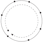
Figure 1: Choice of contour on the interior of the disc.

The sign in the relation derives from the choice of sign in eq. (86). This choice however does not affect the calculation of the amplitudes themselves and hence the relation (89) holds for both choices of sign. Note that the amplitudes are not considered to be real (as in [16, 17]), which is a special choice only available with a definite reality condition on the momenta. As the relations will be used to study BCFW shifts in this paper (which are inherently complex), this is an important property.

Two subtleties

There are two subtleties related to limits within the above argument which will be important in the following. Looking more closely to the process in which the integration contour is taken to the edge of the disc shows that a careful limit argument is necessary, by taking for instance half-arcs around the vertex operator insertions. The integration over these arcs with, say, radius $\epsilon$ can easily be performed by considering the OPE of the ‘stationary’ and the moving vertex operator,

$$\int_{R^{+}_{\epsilon}(z_{i})}dz_{1}\langle:\!V(z_{1})\!::\!V(z_{i})\!:\ldots\rangle =\int_{R_{\epsilon}(z_{i})}\langle\left(z_{1}-z_{i}\right)^{2{\alpha^{\prime}}p_{1}\cdot p_{i}}:\!V(z_{1})V(z_{i})\!:\ldots\rangle$$ (91)

$$=\int_{R_{\epsilon}(z_{i})}dz_{1}\langle\left(z_{1}-z_{i}\right)^{2{\alpha^{\prime}}p_{1}\cdot p_{i}}\sum_{k=0}^{\infty}C_{1ik}(z_{1}-z_{i})^{k}:\!V_{k}\!:\ldots\rangle\ .$$ (92)

Here $C_{1ik}$ are the CFT structure constants. Note that a similar computation yields the leading pole behavior for kinematic limits of particles $1$ and $i$ of the form ${\alpha^{\prime}}(p_{1}+p_{i})^{2}\rightarrow m$ for some integer $m$. The ‘leading singularity’ of the integral is therefore found by considering the coupling of particles $1$ and $i$ to the lowest mass resonance possible in the theory. For bosonic string tachyons for instance this is the tachyon itself.

Since the above formula isolates the singular behavior in the limit $\epsilon\rightarrow 0$ it allows the corresponding integral to be evaluated to give

$$\int_{R^{+}_{\epsilon}(z_{i})}dz_{1}\left(z_{1}-z_{i}\right)^{2{\alpha^{\prime}}p_{1}\cdot p_{i}}\rightarrow\epsilon^{-1-2{\alpha^{\prime}}p_{1}\cdot p_{i}}\int_{0}^{\pi}d\theta e^{\textrm{i}\theta(2{\alpha^{\prime}}p_{1}\cdot p_{i})}\ .$$ (93)

Hence the arc integral vanishes for the open bosonic string tachyon amplitude in the limit $\epsilon\rightarrow 0$ if

$$\mbox{Re~{}}(2{\alpha^{\prime}}p_{1}\cdot p_{i})>1\quad\quad\textrm{if $\theta$ integral finite}\ ,$$ (94)

as long as the angle integral over $\theta$ is finite. In other words, the monodromy relation (89) holds as long as the momentum invariant $p_{1}\cdot p_{i}$ is away from the first resonance that the particles one and $i$ couple to.

Subtlety 1

Based on the above it would seem that the monodromy relation is invalid in the limit where

$$2{\alpha^{\prime}}p_{1}\cdot p_{i}\rightarrow 1\ .$$ (95)

This is exactly the location of the tachyon pole. However, there are two limits here and it might in principle matter in which order they are taken. If first $\epsilon\rightarrow 0$, then the tachyon pole is contained in the string amplitudes since the integration along the edge of the disc is all the way up to the singular point. If first $2{\alpha^{\prime}}p_{1}\cdot p_{i}\rightarrow 1$ is taken, then the pole is in the arc integral and should be accounted for separately. In both cases, the same result is obtained but form different parts of the calculation. Hence there is no order of limits problem for these particular two limits. This is the first of the two subtleties referred to above.

Subtlety 2

A second more serious subtlety has to do with the actual integral over the arc. As referred to above, this integral is assumed to be finite in order to apply the above argument. This assumption can easily be violated when the momenta are taken to (complex) infinity. The result is then a $0$ times $\infty$ type ambiguity. For general BCFW shifts of particle one and $n$ this implies there is only one choice of sign which is allowed, depending on the direction in the complex plane the BCFW limit is taken in. Note that the choice of sign for which the half-arc integrals vanish corresponds to the same choice of sign in the general relations. Hence in general monodromy relations will lead to exponentially suppressed amplitudes for non-adjacent BCFW shifts, without reality conditions. This will be spelled out below.

General monodromy relations

Before studying shifts it is interesting to consider generic applications of the relations. To derive a general result consider

$$\int^{\prime}\prod_{i=1}^{k}\oint_{z_{\alpha_{i}}}H(|z_{\alpha_{i}}-z_{1}|>|z_{\alpha_{i+1}}-z_{1}|)\\ \langle 0|:\!V(z_{\alpha_{1}})\!:\ldots:\!V(z_{\alpha_{k}})\!::\!V_{1}\!::\!V_{\beta_{1}}\!:\ldots:\!V_{\beta_{s}}\!::\!V(z_{n})\!:|0\rangle=0\ ,$$ (96)

and fix the position of operators $1$, $n$ and one of the $\beta$’s. The Heaviside $H$ function forces an ordering of the $\alpha$ particles (operators at $z_{\alpha_{i}}$) with respect to the distance to the first fixed operator. Again, ordering the operators to reproduce the amplitude integrands gives

$$A(\alpha_{1}\ldots\alpha_{r}1\beta_{1}\ldots\beta_{s}n)=\\ (-1)^{r}\left(\prod_{i}e^{\pm(\alpha_{i}1)}\right)\left(\prod_{i>j}e^{\pm(\alpha_{i}\alpha_{j})}\right)\left(\sum_{\sigma\in OP\{\alpha\}^{T}\cup\{\beta\}}\left(\prod_{i=1}^{r}\prod_{j=1}^{s}e^{\pm(\alpha_{i}\beta_{j})}\right)A(1\sigma n)\right)\ ,$$ (97)

in terms of the phase factors in eq. (90). These phase factors depend on the ordering of the particles in the term under study of the sum. The conditions under which this is allowed are unchanged with respect to the analysis above, including the remarks about the subtleties. Note that the same sign should be used for all shuffling operations in the co-cycle factor in eq. (86). This leaves one sign choice in the result (97). These relations show how to express any amplitude into ones with a fixed order of two particles. Using first one sign choice and then the other allows one to find a basis of all amplitudes with three particles in a fixed order. This basis has $(n-3)!$ elements, as shown explicitly in [16].

Derivation by iteration

The same result can also be derived by induction from (89). The possibility of doing this is mentioned in [17]. The base step was proven above. For the induction step assume (97) holds for $(r-1)$ $\alpha$ particles. From (89) the following equation holds by pushing $\alpha_{1}$ through the amplitude,

$$A(\alpha_{1}\ldots\alpha_{r}1\beta_{1}\ldots\beta_{s}n)+e^{\pm(\alpha_{2}\alpha_{1})}A(\alpha_{2}\alpha_{1}\ldots\alpha_{r}1\beta_{1}\ldots\beta_{s}n)+\ldots=\\ -C(\alpha_{1}\ldots\alpha_{r}1\beta_{1}\ldots\beta_{s}n)-e^{\pm(\alpha_{2}\alpha_{1})}C(\alpha_{2}\alpha_{1}\ldots\alpha_{r}1\beta_{1}\ldots\beta_{s}n)+\ldots\ ,$$ (98)

where terms with the same number of particles between $1$ and $n$ have been collected on the left hand side, moving the others to the right. Here $C({\alpha},1,{\beta},n)$ is defined as the right hand side of eq. (97). The terms of the right hand side are split into different orderings of $\alpha_{1}$ amongst the ordered other $\alpha$’s. For every ordering on the right hand side there is a corresponding (inverse) ordering of $\alpha$’s on the left hand side. Indeed, grouping terms shows already (97). By re-labeling the $\alpha$ particles cyclically more equations can be derived, leading to a system of $s$ independent inhomogeneous linear equations in $s$ unknowns. The unique solution of this system reproduces (97). Again, the derivation uses (89) for one choice of sign only.

Extension to fermions

The above argument can also easily be adapted to study monodromy relations for amplitudes which involve fermions. From the field theory point of view examples of these in four dimensions have been discussed in [34]. For this one needs the co-cycle factors

$$:\!V^{f}_{1}(z_{1})\!::\!V^{f}_{2}(z_{2})\!:\equiv-:\!V^{f}_{2}(z_{2})\!::\!V^{f}_{1}(z_{1})\!:e^{i2\pi{\alpha^{\prime}}\left(p_{1}p_{2}\right)\epsilon({z_{1},z_{2}})}\ ,$$ (99)

with an extra minus sign from Fermi statistics, and

$$:\!V_{1}(z_{1})\!::\!V^{f}_{2}(z_{2})\!:\equiv:\!V^{f}_{2}(z_{2})\!::\!V_{1}(z_{1})\!:e^{i2\pi{\alpha^{\prime}}\left(p_{1}p_{2}\right)\epsilon({z_{1},z_{2}})}\ ,$$ (100)

where the superscript indicates if a vertex operator creates a fermionic state or not. The derivation of general relations then proceeds along similar lines to the above, subject to similar reality conditions.

3.3 Non-adjacent shifts from monodromy relations

The study of monodromy relations in the previous section allows an elementary derivation of the non-adjacent shift behavior of string theory amplitudes. For concreteness we first focus on open bosonic string tachyon amplitudes. The first example follows from studying eq. (89) which can be used to shift particles $1$ and $n$ to yield

$$A(\alpha_{1}1\beta_{1}\ldots\beta_{s}n)=e^{\pm\textrm{i}2zqp_{\alpha_{1}}}z^{2{\alpha^{\prime}}p_{1}p_{n}+1}\left(G_{0}+\frac{G_{1}}{z}+\mathcal{O}(z)\right)\ ,$$ (101)

in this expression the $+$ sign should be chosen if $\mbox{Im~{}}(2zqp_{\alpha_{1}})>0$ and the $-$ sign if $\mbox{Im~{}}(2zqp_{\alpha_{1}})<0$. Note that the behavior of the adjacent shift is simply repeated - suppressed by an exponential. In a real sense this equation is an upper limit: the in principle complicated function $G_{0}$ could vanish.

As can be seen from eq. (98) in a case where there are more than $1$ particles between the particles which are shifted, the analysis becomes more complicated. To get a firm grasp of what is needed, let us study the case of two $\alpha$ particles. In this case in principle $4$ types of relations can be derived by pushing either $\alpha_{1}$ or $\alpha_{2}$ through, with two sign choices each. Based on the subtleties mentioned above, only $2$ of these types of relations hold in the large $z$ limit, depending on the sign of the two quantities,

$$\mbox{Im~{}}(2zqp_{\alpha_{1}})\quad,\mbox{Im~{}}(2zqp_{\alpha_{2}})\ .$$

For a fixed choice of sign of these quantities, the two types of relations which do hold involve two unknowns,

$$A(\alpha_{1}\alpha_{2}\hat{1}\beta\hat{n})\quad\textrm{and}\quad A(\alpha_{2}\alpha_{1}\hat{1}\beta\hat{n})\ ,$$ (102)

since the behavior of amplitudes with only one $\alpha$ is known from eq. (101). However, on inspecting it is seen that there are cases where the two equations obtained are degenerate as the large z-shift of the relations read,

$$A(\alpha_{1}\alpha_{2}\hat{1}\beta\hat{n})+e^{\pm_{1}(\alpha_{1}\alpha_{2})}A(\alpha_{2}\alpha_{1}\hat{1}\beta\hat{n})\\ =-e^{\pm_{1}\textrm{i}z2qp_{\alpha_{1}}}e^{\pm_{2}\textrm{i}z2qp_{\alpha_{2}}}z^{2{\alpha^{\prime}}p_{1}p_{n}+1}\left(G_{0}+\frac{G_{1}}{z}+\mathcal{O}(z)\right)\ ,$$ (103)

$$e^{\pm_{2}(\alpha_{2}\alpha_{1})}A(\alpha_{1}\alpha_{2}\hat{1}\beta\hat{n})+A(\alpha_{2}\alpha_{1}\hat{1}\beta\hat{n})\\ =-e^{\pm_{1}\textrm{i}z2qp_{\alpha_{1}}}e^{\pm_{2}\textrm{i}z2qp_{\alpha_{2}}}z^{2{\alpha^{\prime}}p_{1}p_{n}+1}\left(G_{0}+\frac{G_{1}}{z}+\mathcal{O}(z)\right)\ ,$$ (104)

where the choice of signs $(\pm)_{1,2}$ in every contour is such that there is exponential suppression. To get around this the same modification of the integrand as in (97) will yield a relation where the $\alpha_{i}$ particles appear ordered. In particular, there is only one term in the relation with all $\alpha_{i}$ particles between the shifted particles $1$ and $n$, while all the other terms contain adjacent particles $1$ and $n$ only.

This yields for a shift of generically non-adjacent particles $1$ and $j$

$$A(z)\sim e^{2{\alpha^{\prime}}zq\cdot\left(\sum_{i=2}^{j-1}\pm_{i}p_{i}\right)}z^{{\alpha^{\prime}}(p_{1}+p_{j})^{2}}\left(G(z)+\mathcal{O}\left(\frac{1}{z}\right)\right.\ ,$$ (105)

where $G(z)$ starts with the same power of $z$ as the adjacent shift of particles $1$ and $j$ and the signs in the exponential are such that the resulting shift is always exponentially suppressed, regardless of the direction of $z$. This argument holds up to $2((j-1)-1)$ points on the circle at infinity. Excising these and inserting our analyticity argument as before finishes the discussion of non-adjacent shifts, up to one subtlety.

This subtlety has to do with the field theory limit: in this limit the field theory is known to behave one power of $z$ better than the adjacent shift. An argument in the string theory for this which will be substantiated more in the next section is as follows. For the case of one $\alpha$ particle (Next-to-Adjacent shifts) eq. (105) is special. From (101) in the large $z$ limit the non-adjacent shift is related to a sum over terms which look like a monodromy relation again, but now with an ‘effective’ particle made out of the shifted particles, whose momentum is the sum of both. This does not happen for more $\alpha$ particles because of the complicated sign structure. If the leading power can be interpreted as a physical state in the string again, then the leading power of $z$ cancels exactly in this particular case. Below an argument for this from the CFT will be given.

4 OPE derivation of adjacent shifts

The results above for the kinematic constraints for the particle shifts of adjacent gluon legs beg for a more streamlined and above all physical discussion. From the point of view of the string theory, it is natural to suspect that this discussion should be in the language of the underlying CFT. As the analysis for non-adjacent shifts is already in this form, what is needed to complete the CFT picture is the adjacent shift behavior. For four points this is closely related to Regge behavior, which has been analyzed directly from the underlying CFT in [35] for other purposes. Below the approach of that paper is adapted to the case at hand.

4.1 Shifting tachyons

Let us gauge fix operators $2$, $n-1$ and $n$ to $0$, $1$ and $\infty$ respectively for an $n$-particle color-ordered amplitude,

$$A(12\ldots n)\ ,$$ (106)

and consider the shift,

$$p_{1}\rightarrow p_{1}+zq\quad,\quad p_{2}\rightarrow p_{2}-zq\ ,$$ (107)

with the usual constraint (2). The shifted particles will be taken to be tachyons, while the rest of the amplitude is left general. From the OPE of the two open string tachyon vertex operators

$$:\!e^{\textrm{i}\hat{p}_{1}X(y)}\!:\,:\!e^{\textrm{i}\hat{p}_{2}X(0)}\!:=\left(y\right)^{2{\alpha^{\prime}}p_{1}p_{2}}:\!e^{\textrm{i}\left(p_{1}X(y)+p_{2}X(0)\right)+\textrm{i}zq^{\mu}\left(X_{\mu}(y)-X_{\mu}(0)\right)}\!:\ ,$$ (108)

follows which clearly isolates the $z$-dependent part of the integrand. The leading Regge term can [35] be isolated from this expression by Taylor expanding with respect to $y$ in the exponential,

$$:\!e^{\textrm{i}\hat{p}_{1}X(y)}\!:\,:\!e^{\textrm{i}\hat{p}_{2}X(0)}\!:\sim\left(y\right)^{2{\alpha^{\prime}}p_{1}p_{2}}:\!e^{\textrm{i}\left(p_{1}+p_{2}\right)X(0)+\textrm{i}zyq^{\mu}\left(\partial X_{\mu}(0)\right)+\mathcal{O}\left(y^{2}\right)}\!:\ .$$ (109)

Of course, a reasoning is needed to argue that the sub-leading terms in $y$ can be ignored. To obtain the full amplitude the complete correlation function must be calculated and then integrated. One can of course at least formally integrate the above expression directly. From a saddle-point approximation in the expression above a saddle point $y\sim\frac{1}{z}$ is obtained or in other words an effective expansion in terms of $(yz)$. For the purposes of this article this argument will be taken to hold - a more rigorous treatment would be very welcome as this will be our main assumption in this section.

Up to the order indicated the integral over the position of the first particle in the scattering amplitude from $-\infty$ to $0$ can be performed explicitly,

$$\int_{-\infty}^{0}\left(y\right)^{2{\alpha^{\prime}}p_{1}p_{2}} :\!e^{\textrm{i}\left(p_{1}+p_{2}\right)X(0)+\textrm{i}zyq^{\mu}\left(\partial X_{\mu}(0)\right)}\!:\,=$$

$$:\!e^{\textrm{i}\left(p_{1}+p_{2}\right)X(0)}\left(\textrm{i}zq^{\mu}\left(\partial X_{\mu}(0)\right)\right)^{-1-2{\alpha^{\prime}}p_{1}p_{2}}\Gamma(1+2{\alpha^{\prime}}p_{1}p_{2})\!:\ ,$$ (110)

with somewhat abstract reality conditions

$$\mbox{Re~{}}\left({\alpha^{\prime}}p_{1}p_{2}\right)>-1\quad\quad\mbox{Re~{}}(zq\left(\delta X(0)\right))>0\ .$$ (111)

Interestingly the effective operator in eq. (4.1) again looks like a vertex operator for a physical state, apart from the non-familiar exponential. It is not too hard too verify that the operator indeed obeys the physical state conditions as

$$:\!e^{\textrm{i}\left(p_{1}+p_{2}\right)X(0)}\left(\textrm{i}zq^{\mu}\left(\partial X_{\mu}(0)\right)\right)^{-1-2{\alpha^{\prime}}p_{1}p_{2}}\!:|0\rangle\sim\left(q_{\mu}\alpha_{-1}^{\mu}\right)^{-1-2{\alpha^{\prime}}p_{1}p_{2}}|p_{1}+p_{2}\rangle\ ,$$ (112)

This is very similar to the vector excitation in the bosonic string. The physical state conditions reads $q\cdot(p_{1}+p_{2})=0$ which indeed holds. Note that this argument only holds for the leading term in the large $z$ expansion: sub-leading terms will spoil this behavior.

From the above expression the large $z$ behavior of the full amplitude can easily be isolated for the tachyon amplitude in the bosonic string,

$$A_{n}(z)\rightarrow\left(\frac{1}{z}\right)^{{\alpha^{\prime}}(p_{1}+p_{2})^{2}-1}\left(\tilde{G}_{0}+\mathcal{O}\left(\frac{1}{z}\right)\right)\ .$$ (113)

The CFT argument reproduces the adjacent shift behavior found in eq. (30) for adjacent tachyons. Crucially, the evaluation of all remaining contractions in the vacuum expectation value can not depend on $z$. Note that in the CFT argument the shift behavior is manifestly universal: it only depends on the OPE of the shifted vertex operators.

Note also that since the leading term of the large $z$ expansion obeys the physical state condition, it obeys the same braiding relation as in eq. (86). This validates our argument above that non-adjacent shifts are suppressed by one additional power of $z$ compared to the leading one.

4.2 Shifting gluons

The argument above for tachyons can be extended to more general cases such as the shift of adjacent gluons. First this will be analyzed for the bosonic string, after which the RNS formulation of the superstring will be treated. In this subsection we will set ${\alpha^{\prime}}=\frac{1}{2}$, restoring dependence on this parameter by dimensional analysis at the end.

4.2.1 Bosonic string

In the bosonic string the vertex operators for gluons can be written as the part of

$$:\!e^{\textrm{i}p_{1}\cdot X(y_{1})+\zeta_{1}\cdot\partial X(y_{1})}\!:\ ,$$ (114)

which is linear in the external polarization $\zeta_{1}$. The exponential form is convenient for performing contractions, such as for instance for the OPE of two adjacent gluons,

$$:\!e^{\textrm{i}p_{1}\cdot X(y)+\zeta_{1}\cdot\partial X(y)}\!:\,:\!e^{\textrm{i}p_{2}\cdot X(0)+\zeta_{2}\cdot\partial X(0)}\!:\,\quad\sim\quad:\!K\,\,e^{W}\!:\ ,$$ (115)

where in the last line $K$ is the part of the OPE linear in both polarization vectors,

$$K=\zeta_{1}\cdot\partial X(y)\zeta_{2}\cdot\partial X(0)+\frac{\zeta_{1}\cdot\partial X(y)\zeta_{2}\cdot p_{1}-\zeta_{1}\cdot p_{2}\zeta_{2}\cdot\partial X(0)}{y}+\frac{\zeta_{1}\cdot\zeta_{2}+\zeta_{1}\cdot p_{2}\zeta_{2}\cdot p_{1}}{y^{2}}\ ,$$ (116)

and $W$ is the same exponential as in the tachyon case (see eq. (108))

$$W=p_{1}\cdot p_{2}\log y+\textrm{i}\left(p_{1}\cdot X(y)+p_{2}\cdot X(0)\right)\ .$$ (117)

Note that up to this point everything is exact. Now the BCFW shift can be applied as above in eq. (35). The exponential will be Taylor expanded as

$$W\sim p_{1}p_{2}\log y+\textrm{i}\left(p_{1}+p_{2}\right)X(0)+\textrm{i}zyq^{\mu}\left(\partial X_{\mu}(0)\right)+\mathcal{O}\left(y^{2}\right)\ ,$$ (118)

To leading order the integral over $y$ can now be performed explicitly in the same way as above. Therefore for the shift of two adjacent gluons in any open bosonic string amplitude

$$A_{n}(z)=\left(\frac{1}{z}\right)^{2{\alpha^{\prime}}p_{1}p_{2}}\hat{\zeta}_{1}^{\mu}\left[\int_{\textrm{positions}}\langle\Bigg{\{}z\left[\eta_{\mu\nu}+2{\alpha^{\prime}}P_{\mu}P_{\nu}\right]G_{1}+\right.\\ \left.\left[\partial X(0)_{\mu}P_{\nu}-P_{\mu}\partial X(0)_{\nu}\right]G_{2}+\mathcal{O}\left(\frac{1}{z}\right)\Bigg{\}}V_{3}V_{4}\ldots V_{n}\rangle\right]\hat{\zeta}_{2}^{\nu}\ ,$$ (119)

holds, where explicit ${\alpha^{\prime}}$ has been restored. To obtain this expression

$$p_{1}\cdot\zeta_{2}=-P\cdot\zeta_{2}\qquad\qquad p_{2}\cdot\zeta_{1}=-P\cdot\zeta_{1}\ ,$$ (120)

with

$$\sum_{i=3}^{n}p_{i}\equiv P\ ,$$ (121)

was used to eliminate any apparent $z$ dependence in the shifted momenta. The integration in eq. (119) is over the position of particles $3$ through $n-2$. The $G_{i}$ are operator dependent polynomials in $(\frac{1}{z})$ with constant term. The form of eq. (119) is exactly the same as the leading and sub-leading terms in eq. (53). Antisymmetry of the sub-leading term is manifest. Hence the CFT argument reproduces the large shift behavior of Table 2. Again, the CFT argument clearly indicates that the obtained behavior is independent of the particle content of the rest of the amplitude.

Again, the leading term of the large $z$ expansion obeys the physical state condition as above as the leading operator is simply the same. This verifies the claim that non-adjacent shifts are suppressed by one additional power of $z$ compared to the leading one as the full leading behavior is given by this term.

4.2.2 Superstring in the RNS formulation

The vertex operators of the superstring in the RNS formulation can be written as a double Grassmanian integral,

$$V(p,\zeta,y)=\int d\theta d\eta V(\theta,\eta)=\int d\theta d\eta e^{\textrm{i}p_{\mu}X^{\mu}(y)+\eta\theta\zeta_{\mu}\bar{\partial}X^{\mu}(y)+\theta p_{\mu}\psi^{\mu}(y)+\eta\zeta_{\mu}\psi^{\mu}(y)}\ .$$ (122)

The calculation can now be set up completely analogously to the reasoning followed above. Let us first calculate the OPE,

$$:\!V_{1}(p_{1},\zeta_{1},y_{1})\!:\,:\!V_{2}(p_{2},\zeta_{2},y_{2})\!:=\int d\theta_{1}d\eta_{1}d\theta_{2}d\eta_{2}:\!V_{1}(\theta_{1},\eta_{1})V_{2}(\theta_{1},\eta_{1})\!:\\ \exp\left[p_{1}p_{2}\left(\log(y_{2}-y_{1})+\frac{\theta_{1}\theta_{2}}{y_{2}-y_{1}}\right)+\eta_{1}\theta_{1}\eta_{2}\theta_{2}\frac{\zeta_{1}\zeta_{2}}{(y_{2}-y_{1})^{2}}-\eta_{1}\theta_{1}\frac{\zeta_{1}p_{2}}{y_{2}-y_{1}}+\right.\\ \left.\eta_{2}\theta_{2}\frac{p_{1}\zeta_{2}}{y_{2}-y_{1}}+\theta_{1}\eta_{2}\frac{p_{1}\zeta_{2}}{y_{2}-y_{1}}+\eta_{1}\theta_{2}\frac{\zeta_{1}p_{2}}{y_{2}-y_{1}}+\eta_{1}\eta_{2}\frac{\zeta_{1}\zeta_{2}}{y_{2}-y_{1}}\right]\ .$$ (123)

The integrals over the Grassmanian parameters can be performed, which yields the same structure as before,

$$:\!V_{1}(p_{1},\zeta_{1},y_{1})\!:\,:\!V_{2}(p_{2},\zeta_{2},y_{2})\!:=:\!K_{\textrm{susy}}e^{W}\!:\ ,$$ (124)

with $W$ as in eq. (117). The polarization dependent structure can be written as

$$K_{\textrm{susy}}=K_{0}+\frac{K_{1}}{(y_{2}-y_{1})^{1}}+\frac{K_{2}}{(y_{2}-y_{1})^{2}}\ ,$$ (125)

with

$$K_{2} =\left(\zeta_{1}\cdot\zeta_{2}\right)(1+p_{1}p_{2})$$ (126)

$$K_{1} =(\zeta_{1}P)\left[\zeta_{2,\mu}\bar{\partial}X^{\mu}(y_{2})+\zeta_{2,\mu}\psi^{\mu}(y_{2})\left(p_{2,\nu}\psi^{\nu}(y_{2})+p_{1,\nu}\psi^{\nu}(y_{1})\right)\right]-$$

$$\quad\quad(\zeta_{2}P)\left[\zeta_{1,\mu}\bar{\partial}X^{\mu}(y_{1})+\zeta_{1,\mu}\psi^{\mu}(y_{1})\left(p_{1,\nu}\psi^{\nu}(y_{1})+p_{2,\nu}\psi^{\nu}(y_{2})\right)\right]+$$

$$\quad\quad\quad\quad(\zeta_{1}\zeta_{2})\left[p_{1,\mu}p_{2,\nu}\psi^{\mu}(y_{1})\psi^{\nu}(y_{2})\right]+(p_{1}p_{2})\left[\zeta_{1,\mu}\zeta_{2,\nu}\psi^{\mu}(y_{1})\psi^{\nu}(y_{2})\right]$$ (127)

$$K_{0} =\left[\zeta_{1,\mu}\bar{\partial}X^{\mu}(y_{1})+\zeta_{1,\mu}p_{1,\nu}\psi^{\mu}(y_{1})\psi^{\nu}(y_{1})\right]\left[\zeta_{2,\mu}\bar{\partial}X^{\mu}(y_{2})+\zeta_{2,\mu}p_{2,\nu}\psi^{\mu}(y_{2})\psi^{\nu}(y_{2})\right]\ ,$$ (128)

where eq. (120) was used. Compared to the bosonic string the analysis is more complicated since the above expressions contain explicit dependence on $z$ through $p_{1}$ and $p_{2}$. The leading order behavior of the amplitude follows from the above reasoning. The simplest is $K_{2}$. This contributes

$$A(z)_{\textrm{contribution from}K_{2}}\sim\left(\frac{1}{z}\right)^{p_{1}p_{2}-1}\left[\left(\zeta_{1}\cdot\zeta_{2}\right)(1+p_{1}p_{2})\right]\ .$$ (129)

The other two are suppressed with respect to this contribution, $K_{1}$ by $\frac{1}{z}$ and $K_{0}$ by $\frac{1}{z^{2}}$. The strategy now will be to show that leading terms will be proportional to metric contractions between $\zeta_{1}$ and $\zeta_{2}$, while the sub-leading terms are antisymmetric in these two polarizations.

Expanding the integrand in $(y_{2}-y_{1})$ and repeating the integral argument shows that the leading behavior arises from the $K$ factors, evaluated at $y_{2}=y_{1}$. Sub-leading contributions arise from higher order terms in the Taylor expansion in $(y_{2}-y_{1})$. The first two lines of $K_{1}$ are explicitly anti-symmetric. Furthermore, the potentially dangerous $z$-dependence in this factor from the momenta cancels explicitly at leading order in $(y_{2}-y_{1})$. The last line of $K_{1}$ contains one term proportional to the metric which due to the antisymmetry of $\psi\psi$ at leading order in $(y_{2}-y_{1})$ can only contribute at the same order in $z$ as the contribution coming from $K_{2}$. The other term on the last line of $K_{1}$ is explicitly anti-symmetric at leading order in $(y_{2}-y_{1})$.

The remaining $K_{0}$ contribution can only contribute at leading or sub-leading order in $z$ if the $z$ dependence in the momentum would play a role. At leading order in $(y_{2}-y_{1})$ the potentially dangerous terms come from

$$\sim\zeta_{1,\mu}\hat{p}_{1,\nu}\psi^{\mu}\psi^{\nu}\zeta_{2,\kappa}\hat{p}_{2,\rho}\psi^{\kappa}\psi^{\rho}+\zeta_{1,\mu}\bar{\partial}X^{\mu}\zeta_{2,\mu}\hat{p}_{2,\nu}\psi^{\mu}\psi^{\nu}+\zeta_{2,\mu}\bar{\partial}X^{\mu}\zeta_{1,\mu}\hat{p}_{1,\nu}\psi^{\mu}\psi^{\nu}=\\ z\zeta_{1,\mu}\left[\psi^{\kappa}\psi^{\mu}\left(p_{1,\nu}q_{\rho}-q_{\nu}p_{2,\rho}\right)\psi^{\nu}\psi^{\rho}+\left(\bar{\partial}X^{\mu}(q_{\nu}\psi^{\nu})\psi_{\kappa}-\bar{\partial}X^{\kappa}(q_{\nu}\psi^{\nu})\psi_{\mu}\right)\right]\zeta_{2,\kappa}+\mathcal{O}\left(z^{0}\right)\ ,$$ (130)

where the shift has been implemented. These contributions are explicitly anti-symmetric while it can only contribute one order in $z$ higher: at the same level as $K_{1}$. At sub-leading order in $(y_{2}-y_{1})$ the only possible non-zero contribution is anti-symmetric in $\zeta_{1}$ and $\zeta_{2}$ since the derivative has to act on one of the fields contracted into $q_{\mu}\psi^{\mu}$.

Gathering all the terms it is seen that the leading order behavior of the shift of two adjacent gluons in the superstring can be derived from

$$A_{n}\sim\left(\frac{1}{z}\right)^{2{\alpha^{\prime}}(p_{1}\cdot p_{n})}\hat{\zeta}_{1}^{\mu}\left(z\,h_{1}(1+2{\alpha^{\prime}}p_{1}\cdot p_{n})g_{\mu\nu}+\left(h_{2}B_{\mu\nu}\right)+\mathcal{O}\left(\frac{1}{z}\right)\right)\hat{\zeta}_{2}^{\nu}\ ,$$ (131)

where $B$ is an anti-symmetric tensor and $h_{i}$ are some polynomials in $\frac{1}{z}$ with constant finite part. They can be related to certain operators in the CFT as before. In this expression explicit ${\alpha^{\prime}}$ has been restored. The derived formula allows one to reproduce Table 3 from the CFT argument. Just as above, the argument does not depend on the field content of the rest of the amplitude.

As above, for non-adjacent shifts our suppression argument will work as in the bosonic string: the braiding factor is the same. However, here the leading behavior in $z$ is in some cases determined from parts of the effective vertex operator which are either absent or sub-leading in the bosonic string. This happens in those cases which are better behaved compared to the bosonic string. The importance of the sub-leading terms makes it harder to prove the physical state condition in these cases for the superstring. We conjecture, but do not prove, that the same conclusion as there holds: suppression by one power of $z$. Note that this is certainly true in the field theory limit and can be checked to hold for the purely bosonic part.

4.3 Remarks

The CFT argument is seen to yield the same answers as the direct integral analysis as presented in section 2, at least in the cases checked here. The CFT is however remarkably more efficient. Also, in the CFT picture it is obvious that the large $z$ behavior should indeed be universal in string theory in the sense explained above as it only depends on the OPE between the two shifted particles, not on any other leg. The large $z$ behavior of any choice of two species of particle in the open string should also follow most easily from the above CFT argument. This can be seen from the general shape of the DDF vertex operators in the bosonic string [36], as these can be thought of as products of massless vertex operators. For the superstring it would be interesting to see if the OPE argument for the NSR formulation above can be made more straightforwardly in any formulation of the superstring with manifest target space supersymmetry.

Furthermore, non-adjacent shifts are expected to be suppressed with respect to the adjacent shift by application of (89)in general: the leading behavior in $z$ features in effect a universal effective particle made of the adjacent shift of $1$ and $2$. It would be nice to have a general proof of the physical state conditions. This argument yields one power of $z$ suppression however.

5 Sample applications of the CFT argument

5.1 Open strings in a constant B-field background

As mentioned in the introduction, a longer term goal of the research program of which this paper is a part of, is to understand string theory in more general backgrounds than the flat one which was discussed up to now. There is a small but non-trivial list of explicit backgrounds for which string theory can be analyzed completely. An interesting example in this list is open string theory in a non-zero but constant B-field background (see the seminal paper by Seiberg and Witten [37] and references therein).

The results of the present article for disc-level string scattering can easily be generalized to that setting. The crucial observation is that a generic CFT correlation function of open string vertex operators in the nontrivial B-field background can be calculated simply from the flat background case,

$$\langle V_{1}V_{2}\ldots V_{n}\rangle_{B\neq 0}=e^{-\frac{\textrm{i}}{2}\sum_{i<j}p^{\mu}_{i}p_{j}^{\nu}\theta_{\mu\nu}\epsilon(z_{i},z_{j})}\langle V_{1}V_{2}\ldots V_{n}\rangle_{B=0,\eta_{\mu\nu}\rightarrow G_{\mu\nu}}\ .$$ (132)

In this formula the non-commutativity parameter $\theta$ is defined as

$$\theta^{\mu\nu}=-(2\pi{\alpha^{\prime}})^{2}\left(\frac{1}{g+2\pi{\alpha^{\prime}}B}B\frac{1}{g-2\pi{\alpha^{\prime}}B}\right)^{\mu\nu}\ ,$$ (133)

where $g$ is the (flat) closed string metric and $B$ the background B-field. Furthermore, the flat space metric $\eta_{\mu\nu}$ is replaced by the open string metric,

$$G^{\mu\nu}=\left(\frac{1}{g+2\pi{\alpha^{\prime}}B}g\frac{1}{g-2\pi{\alpha^{\prime}}B}\right)^{\mu\nu}\ .$$ (134)

In the field theory limit described in [37] the target space theory reduces to the non-commutative version of Yang-Mills theory. In the limit where $B\rightarrow 0$, the flat space correlation functions are recovered. The string amplitudes follow from the correlation function in the usual way by integration over insertion points as in (87).

Monodromy relations

From the relation to the regular string theory amplitudes it is clear that monodromy relations can be derived for the amplitudes in a non-trivial B-field background. More elegantly, this can be done by deriving the co-cycle factor from the string theory OPE and following the derivation of the monodromy relations above. This yields

$$:\!V_{1}(z_{1})\!:\,:\!V_{2}(z_{2})\!:\equiv:\!V_{2}(z_{2})\!:\,:\!V_{1}(z_{1})\!:e^{\textrm{i}p^{\mu}_{1}p^{\nu}_{2}\left(2\pi{\alpha^{\prime}}G_{\mu\nu}-\theta_{\mu\nu}\right)\epsilon({z_{1},z_{2}})}\ .$$ (135)

Since the co-cycle factor does not depend on the insertion points the derivation in subsection 3.2 can be copied directly. This yields a first monodromy relation between different color-orders as

$$A(\alpha_{1},1,\beta_{1}\ldots\beta_{k},n)_{B}=-\sum_{\sigma\in OP\{\alpha_{1}\}\cup\{\beta\}}e^{\pm(\alpha_{1}1)}\left(\prod_{i=1}^{k}e^{\pm(\alpha_{1}\beta_{i})_{\theta}}\right)A(1,\sigma,n)_{B}\ .$$ (136)

Here we have defined the inner product

$$(\alpha\beta)_{\theta}\equiv\textrm{i}\alpha^{\mu}\beta^{\nu}(2\pi{\alpha^{\prime}}G_{\mu\nu}-\theta_{\mu\nu})\ ,$$ (137)

which enters in the definition (90). Note that similar constraints as above apply for reality conditions of the kinematic invariants for these relations to be valid. Iterating these relations yields the generalization of eq. (97),

$$A(\alpha_{1}\ldots\alpha_{r}1\beta_{1}\ldots\beta_{s}n)=\\ (-1)^{r}\left(\prod_{i}e^{\pm(\alpha_{i}1)_{\theta}}\right)\left(\prod_{i>j}e^{\pm(\alpha_{i}\alpha_{j})_{\theta}}\right)\left(\sum_{\sigma\in OP\{\alpha\}^{T}\cup\{\beta\}}\left(\prod_{i=1}^{r}\prod_{j=1}^{s}e^{\pm(\alpha_{i}\beta_{j})_{\theta}}\right)A(1\sigma n)\right)\ ,$$ (138)

Using both possible choices of sign the amplitude can be ordered further. This expresses any color ordered amplitude in terms of an $(n-3)!$ element basis as in the flat space case. As for the flat space case, the monodromy relations hold for any possible field content of the scattering amplitudes.

On-shell recursion in the presence of a B-field

Recursion relations can be obtained for the string theory amplitudes using the techniques of either section 2 or 4, modulo one subtlety with the phase factor in (132). For a generic BCFW shift this phase factor will diverge wildly. However, the divergence is well-localized in any color ordered amplitude. Shifting particles $i$ and $i+1$, this takes the form

$$\sim e^{zq^{\mu}\theta_{\mu\nu}\left(p_{i}+p_{i+1}\right)^{\nu}}\ .$$ (139)

In other words, consider

$$\oint_{z=0}e^{-zq^{\mu}\theta_{\mu\nu}\left(p_{i}+p_{i+1}\right)^{\nu}}\frac{A(z)}{z}\ ,$$ (140)

instead of eq. (3) as the starting point of the derivation of the BCFW relations. As the exponential is an entire function, this does not introduce additional poles. The behavior of the string amplitudes in the large-$z$ limit is given by the flat space results of Tables 2 and 3, replacing the target space metric by the open string metric $G$ in eq. (134). The analysis is completely parallel, up to and including the fact that only one monodromy relation is valid for a given non-adjacent large-$z$ shift. For this shift the amplitude decays exponentially. Note that the resulting recursion relation simply instructs one to calculate the $B=0$ amplitudes through BCFW recursion, replace the metric by the open string metric and multiply by the phase factor. This reproduces the prescription described in [38].

5.2 Closed strings at the level of the sphere

For string theory in a flat background the vertex operators for the closed string sector are products of left and right moving vertex operators,

$$V^{\textrm{cl}}\left(z,\bar{z},\{p,\xi\}\right)=V_{L}^{\textrm{o}}\left(z,\{p,\zeta^{L}\}\right)V_{R}^{\textrm{o}}\left(\bar{z}\{p,\zeta^{R}\}\right)\ .$$ (141)

Here on the left hand side the $\xi$ are the polarization tensors of the closed string modes, while on the right hand side within the color ordered amplitudes the $\zeta^{L}$ and $\zeta^{R}$ are the polarization tensors of the left and right moving open string modes respectively. These two are related by

$$\xi=\zeta^{L}\otimes\zeta^{R}\ ,$$ (142)

where the symbol $\otimes$ may include algebraic restrictions. For instance for gravitons this simply expresses the graviton polarization tensor in terms of the traceless symmetric product of vector polarizations,

$$h_{\mu\nu}=\frac{1}{2}\left(\zeta^{R}_{\mu}\zeta^{L}_{\nu}+\zeta^{R}_{\nu}\zeta^{L}_{\mu}\right)-\frac{\eta^{\mu\nu}}{D}\left(\zeta^{R}\cdot\zeta^{L}\right)\ .$$ (143)

The above simply shows that for free field theory the spin $2$ representation can be found in the tensor product of $2$ spin $1$ representations. This squaring relation seems special to free field theory. However, as shown by KLT [18] a general relation between closed and open string amplitudes was uncovered which generalizes the free field ’squaring’ relation.

As an example first study four, five and six point amplitudes. The main assumption will be that the KLT relations hold in the form derived in [18] also in the large $z$ limit. Regardless of particle content the KLT relations can be taken to read for four particles,

$$A_{4}^{\textrm{cl}}\left(\{p_{i},\xi_{i}\}\right)=\sin\left(2\pi{\alpha^{\prime}}t\right)\,\,A_{L}^{\textrm{o}}\left(\{p_{1},\zeta^{L}_{1}\},\{p_{2},\zeta^{L}_{2}\},\{p_{3},\zeta^{L}_{3}\},\{p_{4},\zeta^{L}_{4}\}\right)\\ A_{R}^{\textrm{o}}\left(\{p_{1},\zeta^{R}_{1}\},\{p_{3},\zeta^{R}_{3}\},\{p_{2},\zeta^{R}_{2}\},\{p_{4},\zeta^{R}_{4}\}\right)\ .$$ (144)

Hence shifting particles $1$ and $4$ on the closed string amplitude gives immediately the product of the shifts of the two open string amplitudes. If the shifts of the open string amplitudes are known, a precise prediction for the large $z$ behavior is obtained. Note that a shift of particles $1$ and $2$ would lead to the same prediction after using the non-adjacent shift analysis above. For five particles KLT give

$$A_{5}^{\textrm{cl}}\left(\{p_{i},\xi_{i}\}\right)\sim\sin\left(2\pi{\alpha^{\prime}}p_{1}\cdot p_{2}\right)\sin\left(2\pi{\alpha^{\prime}}p_{3}\cdot p_{4}\right)\,\,A_{L}^{\textrm{o}}\left(13245\right)A_{R}^{\textrm{o}}\left(31425\right)+\\ \sin\left(2\pi{\alpha^{\prime}}p_{1}\cdot p_{3}\right)\sin\left(2\pi{\alpha^{\prime}}p_{2}\cdot p_{4}\right)\,\,A_{L}^{\textrm{o}}\left(12345\right)A_{R}^{\textrm{o}}\left(21435\right)\ ,$$ (145)

where the tensor structure in the open string amplitudes has been suppressed for notational clarity on the right hand side. Shifting particles $1$ and $5$ shows as above a nice cancelation of the exponential factors between the sine functions and the amplitudes through the use of the non-adjacent shift of eq. (105). A similar conclusion holds for the six-point formula given in [18]. For arbitrary multiplicity KLT give

$$A_{n}^{\textrm{cl}}\left(\{p_{i},\xi_{i}\}\right)\sim\sum_{P,P^{\prime}}A_{L}^{\textrm{o}}\left(P\right)A_{R}^{\textrm{o}}\left(P\right)e^{\textrm{i}\pi F(P,P^{\prime})}\ ,$$ (146)

where the sum is over all permutations $P$ and $P^{\prime}$ of $1,\ldots n-1$ such that $1$ appears before $n-1$. The phase factor is determined from the ordering between pairs of particles in $P$ and $P^{\prime}$

$$F(P,P^{\prime})=\sum_{i,i^{\prime}=1}^{n-1}f(i,i^{\prime})\ ,$$ (147)

with

$$f(i,i^{\prime})=\left(\begin{array}[]{ccl}0&&\textrm{if particles }\{i,i^{\prime}\}\textrm{ same ordering in }\{P,P^{\prime}\}\\ 2\pi{\alpha^{\prime}}p_{i}\cdot p_{i^{\prime}}&&\textrm{if particles }\{i,i^{\prime}\}\textrm{ different ordering in }\{P,P^{\prime}\}\end{array}\right.\ .$$ (148)

Again assuming that the derivation of the KLT relations is unaltered by the shift, the same conclusion as above follows: the large $z$ behavior of the closed string amplitude is the square of the open string one. Indeed, the only thing which could spoil this is the phase factor which can diverge under a large $z$ shift. Without loss of generality, let us shift particles $1$ and $n$. The only source for a potential divergence is then the case where particle $1$ appears with opposite order in the left and right sector open string amplitudes compared to some other particle, say $j$. Schematically this contribution reads

$$\sim e^{\textrm{i}2\pi{\alpha^{\prime}}p_{i}\cdot p_{1}}A(\ldots 1\ldots j\ldots n)A(\ldots j\ldots 1\ldots n)\ .$$ (149)

The divergent phase is then canceled by the phase factor arising from the non-adjacent shift derived above in eq. (105). This reasoning can be repeated for any particle, completing the derivation. Let us stress that this argument relies on the validity of the KLT relations under the shift. Even disregarding applications to recursions, it would be interesting to find a completely CFT based derivation of the KLT relations along the lines of the derivation of the monodromy relations discussed above.

Shifting gravitons

Up to now these results hold for any Lorentz quantum numbers of the external states. It is interesting to specialize to the case of gravitons. Combining our results for the gluonic amplitudes (tables 2 and 3) tables 4 and 5 are obtained for the shift of two gravitons in the bosonic and superstring cases. These tables are again claimed to be universal and in particular to hold for all multiplicities. Again, the different possibilities for the transverse polarization are related to whether or not the different transverse polarizations in the problem are orthogonal.

$\xi_{1}\;\backslash\;\xi_{n}$	$--$	$-+$	$++$	$-$T	$+$T	TT
$--$	$-2$	$0$	$+2$	$0$	$+2$	$+2$
$-+$	$-4$	$-2$	$0$	$-2$	$0$	$0$
$++$	$-6$	$-4$	$-2$	$-4$	$-2$	$-2$
$-$T	$-2$	$0$	$+2$	$-2/-1$	$0/+1$	$0/+1$
$+$T	$-4$	$-2$	$0$	$-3/-4$	$-2/-1$	$-2/-1$
TT	$-2$	$0$	$+2$	$-2/-1$	$0/+1$	$-2/-1/0$

Table 4: Conjectured leading power in $z^{-2{\alpha^{\prime}}(p_{1}+p_{n})^{2}-\kappa}$ for the large $z$ limit of the shift of two gravitons in the bosonic string for all possible polarizations.

$\xi_{1}\;\backslash\;\xi_{n}$	$--$	$-+$	$++$	$-$T	$+$T	TT
$--$	$+2$	$+2$	$+2$	$+2$	$+2$	$+2$
$-+$	$-2$	$-2$	$+2$	$-2$	$0$	$0$
$++$	$-6$	$-2$	$+2$	$-4$	$0$	$-2$
$-$T	$0$	$0$	$+2$	$0/+1$	$0/+1$	$0/+1$
$+$T	$-4$	$-2$	$0$	$+1$	$0/+1$	$-2/-1$
TT	$-2$	$0$	$+2$	$+1$	$0/+1$	$-2/-1/0$

Table 5: Conjectured leading power in $z^{-2{\alpha^{\prime}}(p_{1}+p_{n})^{2}-\kappa}$ for the large $z$ limit of the shift of two gravitons in the superstring for all possible polarizations.

As an argument for tables 4 and 5, consider the closed string version of the CFT argument for the large z-behavior explored above. This follows from [35] quite directly. For the OPE one considers

$$:\!V^{\textrm{cl}}\left(w_{1},\bar{w}_{1}\right)\!:\,:\!V^{\textrm{cl}}\left(w_{2},\bar{w}_{2}\right)\!:=\left[:\!V_{L}^{\textrm{o}}\left(w_{1}\right)\!:\,:\!V_{L}^{\textrm{o}}\left(w_{2}\right)\!:\right]\,\left[:\!V_{R}^{\textrm{o}}\left(\bar{w}_{1}\right)\!:\,:\!V_{R}^{\textrm{o}}\left(\bar{w}_{2}\right)\!:\right]\ .$$ (150)

The saddle point in the integral is at $z(w_{1}-w_{2})\sim z(\bar{w}_{1}-\bar{w}_{2})\sim 1$. Fixing $w_{2}=0=\bar{w}_{2}$, the remaining integral over $w_{1}$ and $\bar{w}_{1}$ over the full complex plane can be performed on the formal level at least by analytic continuation to disentangle both integrals. However, this will yield simply the product of the open string analysis in both left and right sector performed above. As in the open string case, a full justification of the CFT argument will not be given here.

In the case of shifted gravitons the CFT argument leads to the tables 4 and 5 in the bosonic and superstring respectively. The worse behavior of the bosonic string amplitudes compared to the superstring is just as in the gluon case down to terms proportional to ${\alpha^{\prime}}$. Taking this into account, both have a smooth field theory limit. In the field theory the terms proportional to ${\alpha^{\prime}}$ which appear in the bosonic string probably correspond to the known ${\alpha^{\prime}}R^{2}$ and ${\alpha^{\prime}}^{2}R^{3}$ terms in the effective action which are known to be absent in the superstring. A direct field theory argument here seems difficult however.

6 Discussion and conclusion

In a precise sense, the recursion relations explored in this article show that the integrand in the string theory amplitude is a complete derivative: the full string amplitude can be determined from the singular behavior on the boundary of the moduli space of the amplitude. Interestingly, for a chosen shift only part of the boundary behavior is necessary. Different BCFW shifts which use different parts of the boundary lead to different expressions for the same amplitude. These different expressions are all equivalent, a fact which has recently been discussed in [39] and [40] from the field theory point of view. In string theory, this is not a bug but a feature. The equivalence of these different expressions is an exact expression of old-school Dolen-Horn-Schmid [41] ‘duality’ (sometimes also called crossing symmetry). The proof of the recursion relations depends on the complexified high energy Regge behavior of a pair of particles. On-shell recursion therefore seems to be a consequence of the ‘high energy symmetry algebra’ of the string theory [42].

Knowledge of the full string three-point amplitude and the on-shell recursion relation suffice to calculate higher point amplitudes in a flat background at least in principle. In a sense, the recursion relations must be an associativity condition in a topological theory while the three-point functions are structure constants, perhaps along the lines of [43]. Further thought along these lines might lead one to investigate string field theory, especially Witten’s cubic open bosonic string field theory. Note that off-shell Berends-Giele [44] type recursion relations (which involve a current instead of an amplitude) have been studied for open string field theory in [45] and for closed string field theory in [46]. Relating supersymmetric string field theory to the on-shell recursion relations should be very interesting since on-shell recursion avoids any problems with contact terms.

As a tool for practical calculation the on-shell recursion relations are not effective as of yet. Although in principle three particle interactions are fixed by the usual string analysis, especially at higher mass levels the resulting three-point functions are in their current form not very transparent for our purposes (See e.g. [47] and references therein). It would be very interesting to study these using the four dimensional (massive) spinor helicity formalism or even better its higher dimensional extension [25] (see also [48]). It would also be interesting to use the higher dimensional supersymmetric coherent states constructed in [25] to apply the higher dimensional version of the super-shift [7] to string amplitudes. In four dimensions this can be done straightforwardly for massless particles by application of the results of this article. It would also be very interesting to study the interplay between the large $z$ behavior and the ${\alpha^{\prime}}$ expansion.

There are several broader directions in which the research presented in this article could be pursued further.

General backgrounds?

Since the above is (the beginning of) a CFT understanding of on-shell recursion and a real derivation of amplitude relations solely from the CFT, an immediate question is whether or not these observations generalize to string theories in a different setting such as in other backgrounds. One example of this is a constant Abelian vector field background, which will feature in [49]. More generally, it would be highly interesting to study the AdS background in the superstring: the OPE tool developed above was after all inspired by [35] which mainly focused on Regge behavior in the curved background.

In this vein we would like to make an intriguing observation. In general the open string vertex operators obey a braiding relation,

$$:\!V_{1}(z_{1})\!:\,\,:\!V_{2}(z_{2})\!:\,\,\equiv\,\,:\!V_{2}(z_{2})\!:\,:\!V_{1}(z_{1})\!:\,R_{12}\ ,$$ (151)

which is the generalization of the flat background relation (86) where the matrix $R_{12}$ is simply a phase. Now it is known since [50, 51] that consistency of the three point function requires the matrix $R_{12}$ to obey the Yang-Baxter equation. This is trivially true in a flat background, see e.g. [52] for examples in non-flat backgrounds. That relation was crucial in the derivation of the amplitude relations for different color orders, but apart from this the only ingredient was the generic structure of the integration domains. This observation provides a direct link of amplitudes to integrability issues, and it would be very interesting to explore this link further.

String loops?

The CFT understanding of recursion also begs for the question if similar observations can be extended to the string loop level. In fact, from the CFT argument it is at least ‘hand-wavingly obvious’ this is the case, and it would be exceedingly interesting to make this more precise. The main difference to the tree level case is the appearance of branch cuts in the $z$ plane, in addition to closed string poles. An analyticity argument could be used to excise certain points from the contour at infinity at the tree level, but at loop level this is no longer true. Instead, one obtains integrals around the branch cuts which measure the discontinuity across the branch cut. This can be related to amplitudes with a lower amount of loops or legs at least in principle. Note the close relation of this with the ‘sewing construction’ for the correlation functions of any CFT at higher loops.

Loop level recursion in string theory would certainly be interesting with a view of applications to field theory, where it seems prohibitively difficult to obtain the large $z$ behavior in full generality for the (dimensionally regulated) amplitude. Based on a known field theory example in [53], a tension can be expected between the various limits (${\alpha^{\prime}}\rightarrow 0$, $D\rightarrow 4$ and $z\rightarrow\infty$ ) at least for the non-supersymmetric case.

An amplitude bootstrap?

Related to the previous two points, the equivalence of the different recursion relations for string theory amplitudes at tree level is highly reminiscent of the bootstrap equations in conformal field theory. The analogy of possible recursion relations for amplitudes at loop level to the calculation of CFT correlation functions through the sewing construction was also mentioned above. The difference is that in CFT the bootstrap idea applies to the (un-integrated) correlation functions, while for the amplitudes these functions must be integrated over the moduli space. Still, it would be very interesting to make the analogy to the CFT bootstrap more precise. In its most extreme form it would give an equation for the S-matrix, the solution of which forms the space of all string theory amplitudes.

The B-field example however shows already that some care might be required in order to properly obtain the right formulae. In particular the modification of the derivation in eq. (140) stands out here. A preliminary version of the bootstrap idea as applied to field theory was presented in [54].

Finally,

it is an encouraging sign that the recent spectacular progress in field theory can be matched by the string theory, at least as far as on-shell recursion for tree amplitudes is concerned. After all string theory should be an upgrade of field theory, not a downgrade. This article should be taken as inspiration to further study the fruitful interplay between string and field theory techniques.

Appendix A Four-gluon amplitude in bosonic and superstring theory

As an explicit example and cross-check on our results in this appendix BCFW shifts of the four-gluon amplitude in bosonic and type I superstring theory will be discussed. Particles $1$ and $2$ will be shifted.

The four-gluon amplitude

The four-gluon amplitude in the open bosonic strings can be found in for instance [18]. Introducing standard Mandelstam variables $s=-(p_{1}+p_{2})^{2}$, $t=-(p_{1}+p_{4})^{2}$ and $u=-(p_{1}+p_{3})^{2}$ and restoring ${\alpha^{\prime}}$ factors the amplitude can be written as

$$A_{4}(p_{1},\zeta_{1};p_{2},\zeta_{2};p_{3},\zeta_{3};p_{4},\zeta_{4})=\frac{\Gamma(-{\alpha^{\prime}}s-1)\Gamma(-{\alpha^{\prime}}t-1)}{\Gamma({\alpha^{\prime}}u+2)}\mathcal{K}(p_{1},\zeta_{1};p_{2},\zeta_{2};p_{3},\zeta_{3};p_{4},\zeta_{4})\ .$$ (152)

Here $\mathcal{K}$ is a cumbersome kinematic factor

$$\mathcal{K}(p_{1},\zeta_{1};p_{2},\zeta_{2};p_{3},\zeta_{3};p_{4},\zeta_{4})=\\ ({\alpha^{\prime}}s+1)({\alpha^{\prime}}t+1)({\alpha^{\prime}}u+1)\left[-K^{\text{(sup)}}+K^{(s)}+K^{(t)}+K^{(u)}+K^{(stu)}\right]\ ,$$ (153)

$$\begin{split}K^{\text{(sup)}}&=-{\alpha^{\prime}}^{2}(st\zeta_{1}\cdot\zeta_{3}\zeta_{2}\cdot\zeta_{4}+su\zeta_{2}\cdot\zeta_{3}\zeta_{1}\cdot\zeta_{4}+tu\zeta_{1}\cdot\zeta_{2}\zeta_{3}\cdot\zeta_{4})\\ &+2{\alpha^{\prime}}^{2}s(\zeta_{1}\cdot p_{4}\zeta_{3}\cdot p_{2}\zeta_{2}\cdot\zeta_{4}+\zeta_{2}\cdot p_{3}\zeta_{4}\cdot p_{1}\zeta_{1}\cdot\zeta_{3}+\zeta_{1}\cdot p_{3}\zeta_{4}\cdot p_{2}\zeta_{2}\cdot\zeta_{3}+\zeta_{2}\cdot p_{4}\zeta_{3}\cdot p_{1}\zeta_{1}\cdot\zeta_{4})\\ &+2{\alpha^{\prime}}^{2}t(\zeta_{2}\cdot p_{1}\zeta_{4}\cdot p_{3}\zeta_{3}\cdot\zeta_{1}+\zeta_{3}\cdot p_{4}\zeta_{1}\cdot p_{2}\zeta_{2}\cdot\zeta_{4}+\zeta_{2}\cdot p_{4}\zeta_{1}\cdot p_{3}\zeta_{3}\cdot\zeta_{4}+\zeta_{3}\cdot p_{1}\zeta_{4}\cdot p_{2}\zeta_{2}\cdot\zeta_{1})\\ &+2{\alpha^{\prime}}u^{2}(\zeta_{1}\cdot p_{2}\zeta_{4}\cdot p_{3}\zeta_{3}\cdot\zeta_{2}+\zeta_{3}\cdot p_{4}\zeta_{2}\cdot p_{1}\zeta_{1}\cdot\zeta_{4}+\zeta_{1}\cdot p_{4}\zeta_{2}\cdot p_{3}\zeta_{3}\cdot\zeta_{4}+\zeta_{3}\cdot p_{2}\zeta_{4}\cdot p_{1}\zeta_{1}\cdot\zeta_{2})\ ,\end{split}$$ (154)

$$\begin{split}K^{(s)}&=4{\alpha^{\prime}}^{3}s\Bigg{\{}\zeta_{1}\cdot p_{3}\zeta_{2}\cdot p_{3}(\zeta_{3}\cdot p_{1}\zeta_{4}\cdot p_{1}+\zeta_{3}\cdot p_{2}\zeta_{4}\cdot p_{2})+\frac{1}{3}(\zeta_{1}\cdot p_{2}\zeta_{2}\cdot p_{3}\zeta_{3}\cdot p_{1}-\zeta_{1}\cdot p_{3}\zeta_{2}\cdot p_{1}\zeta_{3}\cdot p_{2})\\ &\times(\zeta_{4}\cdot p_{1}-\zeta_{4}\cdot p_{2})\Bigg{\}}\ ,\end{split}$$ (155)

$$\begin{split}K^{(t)}&=4{\alpha^{\prime}}^{3}t\Bigg{\{}\zeta_{2}\cdot p_{1}\zeta_{3}\cdot p_{1}(\zeta_{1}\cdot p_{3}\zeta_{4}\cdot p_{3}+\zeta_{1}\cdot p_{2}\zeta_{4}\cdot p_{2})+\frac{1}{3}(\zeta_{1}\cdot p_{3}\zeta_{2}\cdot p_{1}\zeta_{3}\cdot p_{2}-\zeta_{1}\cdot p_{2}\zeta_{2}\cdot p_{3}\zeta_{3}\cdot p_{1})\\ &\times(\zeta_{4}\cdot p_{3}-\zeta_{4}\cdot p_{2})\Bigg{\}}\ ,\end{split}$$ (156)

$$\begin{split}K^{(u)}&=4{\alpha^{\prime}}^{3}u\Bigg{\{}\zeta_{1}\cdot p_{2}\zeta_{3}\cdot p_{2}(\zeta_{2}\cdot p_{1}\zeta_{4}\cdot p_{1}+\zeta_{2}\cdot p_{3}\zeta_{4}\cdot p_{3})+\frac{1}{3}(\zeta_{1}\cdot p_{2}\zeta_{2}\cdot p_{3}\zeta_{3}\cdot p_{1}-\zeta_{1}\cdot p_{3}\zeta_{2}\cdot p_{1}\zeta_{3}\cdot p_{2})\\ &\times(\zeta_{4}\cdot p_{3}-\zeta_{4}\cdot p_{1})\Bigg{\}}\ ,\end{split}$$ (157)

$$\begin{split}K^{(stu)}&={\alpha^{\prime}}^{2}st\left[\frac{1}{{\alpha^{\prime}}u+1}(\zeta_{1}\cdot\zeta_{3}-2{\alpha^{\prime}}\zeta_{1}\cdot p_{3}\zeta_{3}\cdot p_{1})(\zeta_{2}\cdot\zeta_{4}-2{\alpha^{\prime}}\zeta_{2}\cdot p_{4}\zeta_{4}\cdot p_{2})-(\zeta_{1}\cdot\zeta_{3}\zeta_{2}\cdot\zeta_{4})\right]\\ &+(3\leftrightarrow 2)+(3\leftrightarrow 4)\ ,\end{split}$$ (158)

The factor $K^{\text{(sup)}}$ is the same as it appears in the analogous type I superstring computation. Note that both $\mathcal{K}$ and $K^{\text{(sup)}}$ are $stu$ symmetric so we do not need to compute every term explicitly.

The contribution of the $\Gamma$ factor in (152) coming from the shift $p_{1}\to p_{1}+zq\,,p_{2}\to p_{2}-zq$ is easily derived by considering that (152) itself is nothing but a shifted Beta function, as we already computed in (18). There are however extra powers of ${\alpha^{\prime}}$ and $z$ here to take care of. They are crucial indeed as they give an effective ${\alpha^{\prime}}z$ expansion

$$\frac{\Gamma(-{\alpha^{\prime}}s-1)\Gamma(-{\alpha^{\prime}}t-1)}{\Gamma({\alpha^{\prime}}u+2)}=\frac{\Gamma(-{\alpha^{\prime}}s-1)\Gamma(-{\alpha^{\prime}}t-1)}{({\alpha^{\prime}}u-2)({\alpha^{\prime}}u-1)({\alpha^{\prime}}u)({\alpha^{\prime}}u+1)\Gamma({\alpha^{\prime}}u-2)}\\ \sim\left(\frac{1}{2{\alpha^{\prime}}zq\cdot p_{4}}\right)^{{\alpha^{\prime}}s-1}\frac{1}{(q\cdot p_{4})^{4}{\alpha^{\prime}}^{4}z^{4}}\left[1+\frac{1}{2}{\alpha^{\prime}}z+\mathcal{O}({\alpha^{\prime}}^{2}z^{2})\right]\Gamma({\alpha^{\prime}}s-1)\ .$$ (159)

Now, shifting particles 1 and 2 according to (35) we get the explicit scaling behavior of the complete kinematic factor for any different choice of the polarization vectors associated with shifted momenta. To actually get the correct contributions, an expansion in powers of ${\alpha^{\prime}}$ is needed as well. Sub-leading contributions (in ${\alpha^{\prime}}$), corresponding in the field theory limit to ${\alpha^{\prime}}F^{3}$ and higher corrections, may also differ from the picture in Table 2. The “good” and “bad” shifts for the bosonic string read

$$\mathcal{K}^{+-}\sim-16{\alpha^{\prime}}^{4}\left(2{\alpha^{\prime}}^{2}(q\cdot q^{*})^{2}-\frac{{\alpha^{\prime}}s}{2}\right)(q\cdot p_{4})^{4}\left(\zeta_{3}\cdot\zeta_{4}-2{\alpha^{\prime}}k_{3}\cdot\zeta_{4}k_{4}\cdot\zeta_{3}\right)z^{6}+\mathcal{O}(z^{5})\ ,$$ (160)

$$\mathcal{K}^{-+}\sim 8{\alpha^{\prime}}^{4}{\alpha^{\prime}}s({\alpha^{\prime}}s-1)(q\cdot p_{4})^{4}\left(\zeta_{3}\cdot\zeta_{4}-2{\alpha^{\prime}}k_{3}\cdot\zeta_{4}k_{4}\cdot\zeta_{3}\right)z^{2}+\mathcal{O}(z)\ .$$ (161)

For $++$ and $--$ additional terms appear carrying a higher power of $z$ than expected. However note that these terms also carry additional powers of ${\alpha^{\prime}}$. Anyway it does not seem to be an order of limit problem, since the field theory limiting behavior of the string theory amplitude is obtained by first taking the zero slope limit and then sending $z\to\infty$. Higher corrections carry extra ${\alpha^{\prime}}$ factors that do not cancel with the denominator of (159), this in turn guarantees that the relations in Table 2 are not spoiled.

$$\begin{split}\mathcal{K}^{++}\sim&-4{\alpha^{\prime}}^{4}s(q\cdot p_{4})^{2}\left(q\cdot q^{*}\zeta_{3}\cdot\zeta_{4}-2p_{2}\cdot\zeta_{3}p_{2}\cdot\zeta_{4}\right)z^{2}\\ &+16s{\alpha^{\prime}}^{6}z^{4}(q\cdot p_{4})^{4}(\zeta_{3}\cdot\zeta_{4})+\mathcal{O}({\alpha^{\prime}}^{6}z^{3})\end{split}\ ,$$ (162)

$$\begin{split}\mathcal{K}^{--}\sim&-4{\alpha^{\prime}}^{4}s(q\cdot p_{4})^{2}\left(q\cdot q^{*}\zeta_{3}\cdot\zeta_{4}-2p_{1}\cdot\zeta_{3}p_{1}\cdot\zeta_{4}\right)z^{2}\\ &+16s{\alpha^{\prime}}^{6}z^{4}(q\cdot p_{4})^{4}(\zeta_{3}\cdot\zeta_{4})+\mathcal{O}({\alpha^{\prime}}^{6}z^{3})\end{split}\ .$$ (163)

For transverse polarization vectors we can pick both $\zeta_{1}$ and $\zeta_{2}$ to be along the same transverse direction, indicated with $T$, or chose different directions $T_{1}$ and $T_{2}$ so that $\zeta_{1}^{T1}\cdot\zeta_{2}^{T2}=0$. As in field theory, the latter shift is better behaved than the former by one power of $z$.

$$\mathcal{K}^{TT}\sim 16{\alpha^{\prime}}^{4}z^{4}(q\cdot p_{4})^{4}\zeta_{1}^{T}\cdot\zeta_{2}^{T}(\zeta_{3}\cdot\zeta_{4}-2{\alpha^{\prime}}p_{3}\cdot\zeta_{4}p_{4}\cdot\zeta_{3})+\mathcal{O}(z^{3})\ ,$$ (164)

$$\mathcal{K}^{T1T2}\sim 16{\alpha^{\prime}}^{4}z^{3}(q\cdot p_{4})^{3}(p_{3}\cdot\zeta_{1}^{T1}p_{4}\cdot\zeta_{2}^{2T}-p_{4}\cdot\zeta_{1}^{T1}p_{3}\cdot\zeta_{2}^{2T})\ .$$ (165)

Type I superstrings

In the type I superstring case the four-gluon amplitude has the same structure as (152) with the restriction on the kinematic coefficient being [56, 18]:

$$\mathcal{K}=-({\alpha^{\prime}}s+1)({\alpha^{\prime}}t+1)({\alpha^{\prime}}u+1)K^{\text{sup}}\ .$$ (166)

The large $z$ scaling behavior of this amplitude can be computed the same way as before and leads to

$$\mathcal{K}^{+-}\sim 8{\alpha^{\prime}}^{5}s(q\cdot p_{4})^{4}({\alpha^{\prime}}s+1)\zeta_{3}\cdot\zeta_{4}z^{6}+\mathcal{O}(z^{5})\ ,$$ (167)

$$\mathcal{K}^{-+}\sim 8{\alpha^{\prime}}^{5}s(q\cdot p_{4})^{4}({\alpha^{\prime}}s+1)\zeta_{3}\cdot\zeta_{4}z^{2}+\mathcal{O}(z)\ .$$ (168)

In both the $++$ and $--$ case there are some cancelations to take into account to get the correct large $z$ behavior of the kinematic factors. Such cancelations are due to our particular choice of a Lorentz frame where $s=2p_{1}\cdot p_{2}=2$ and $q\cdot q^{*}=1$, however this only implies a smart choice of unit of measure, which indeed is always possible. Gathering factors that depend on $s-2q\cdot q^{*}$ the kinematic factor for $++$ polarizations reads

$$\begin{split}\mathcal{K}^{++}\sim&8{\alpha^{\prime}}^{5}(s-2q\cdot q^{*})(q\cdot p_{4})^{3}(p_{2}\cdot\zeta_{3}p_{3}\cdot\zeta_{4}-p_{3}\cdot\zeta_{3}p_{2}\cdot\zeta_{4})z^{3}+\\ &4{\alpha^{\prime}}^{5}(q\cdot p_{4})^{2}\Bigg{[}(s-2qq^{*})(s+3t)(p_{2}\cdot\zeta_{3}p_{3}\cdot\zeta_{4}-p_{2}\cdot\zeta_{4}p_{4}\cdot\zeta_{3})\\ &-2sqq^{*}p_{2}\cdot\zeta_{3}p_{3}\cdot\zeta_{4}-s^{2}p_{2}\cdot\zeta_{4}p_{4}\cdot\zeta_{3}+sup_{1}\cdot\zeta_{3}p_{2}\cdot\zeta_{4}\\ &+stp_{1}\cdot\zeta_{4}p_{2}\cdot\zeta_{3}+s\zeta_{3}\cdot\zeta_{4}(q\cdot p_{4}q^{*}\cdot p_{4}+\frac{1}{4}tu)\Bigg{]}z^{2}+\mathcal{O}(z)\end{split}\ .$$ (169)

Letting $s-2q\cdot q^{*}=0$ the factor proportional to $z^{3}$ cancels and the term in $z^{2}$ also gets simplified. The computation for the $--$ case is completely analogous.

$$\begin{split}\mathcal{K}^{++}\sim&4{\alpha^{\prime}}^{5}(q\cdot p_{4})^{2}\Bigg{[}4p_{3}\cdot\zeta_{4}p_{4}\cdot\zeta_{3}+\zeta_{3}\zeta_{4}(2t+t^{2}-4q\cdot p_{4}q^{*}\cdot p_{4})-4p_{2}\cdot\zeta_{3}p_{3}\cdot\zeta_{4}\\ &+2(t+2)p_{1}\cdot\zeta_{3}p_{2}\cdot\zeta_{4}+2tp_{1}\cdot\zeta_{4}p_{2}\cdot\zeta_{3}+4p_{1}\cdot\zeta_{3}p_{4}\cdot\zeta_{3}\Bigg{]}z^{2}+\mathcal{O}(z)\end{split}\ ,$$ (170)

$$\begin{split}\mathcal{K}^{--}\sim&4{\alpha^{\prime}}^{4}(q\cdot p_{4})^{2}\Bigg{[}4p_{3}\cdot\zeta_{4}p_{4}\cdot\zeta_{3}+\zeta_{3}\zeta_{4}(2t+t^{2}-4q\cdot p_{4}q^{*}\cdot p_{4})-4p_{2}\cdot\zeta_{3}p_{3}\cdot\zeta_{4}\\ &+2(t+2)p_{1}\cdot\zeta_{3}p_{2}\cdot\zeta_{4}+2tp_{1}\cdot\zeta_{4}p_{2}\cdot\zeta_{3}+4p_{1}\cdot\zeta_{3}p_{4}\cdot\zeta_{3}\Bigg{]}z^{2}+\mathcal{O}(z)\end{split}\ .$$ (171)

Again, if we choose transverse polarization vectors for $\zeta_{1}$ and $\zeta_{2}$ not to be the same, say along $T_{1}$ and $T_{2}$ ranging in the subset of $d-4$ transverse directions, the kinematic factor is better behaved by one power of $z$

$$\mathcal{K}^{TT}\sim-16{\alpha^{\prime}}^{4}({\alpha^{\prime}}s+1)z^{4}(q\cdot p_{4})^{4}\zeta_{1}^{T}\cdot\zeta_{2}^{T}\zeta_{3}\cdot\zeta_{4}+\mathcal{O}(z^{3})\ ,$$ (172)

$$\begin{split}\mathcal{K}^{T1T2}\sim&16{\alpha^{\prime}}^{4}({\alpha^{\prime}}s+1)z^{3}(q\cdot p_{4})^{3}\Bigg{(}\zeta_{1}^{T1}\cdot\zeta_{4}\zeta_{2}^{T2}\cdot\zeta_{3}+\zeta_{1}^{T1}\cdot\zeta_{3}\zeta_{2}^{T2}\cdot\zeta_{4}\\ &+{\alpha^{\prime}}(p_{4}\cdot\zeta_{1}^{T1}p_{3}\cdot\zeta_{1}^{T2}+p_{3}\cdot\zeta_{1}^{T1}p_{4}\cdot\zeta_{1}^{T2})\zeta_{3}\cdot\zeta_{4}\Bigg{)}+\mathcal{O}(z^{2})\end{split}\ .$$ (173)

Appendix B Anti-symmetry of sub-leading terms in the superstring

In this appendix it will be shown that the tensor structure $B^{2}_{\mu\nu}$ in (72) is anti-symmetric in the Lorentz labels as advertised. This structure arises from the sub-leading contributions in $z$ in eq. (69). Although the leading terms are easy to isolate, the sub-leading ones require quite some more work. To start, note that any term proportional $\zeta_{1}\cdot\zeta_{n}$ can be dropped at the outset as these can be absorbed immediately into an already known contribution. Both $\eta_{n}$ and $\theta_{n}$ need to be integrated over. Sub-leading ($\frac{1}{z}$ compared to leading) contributions in $\frac{1}{z}$ arise from terms with either $\theta_{i}$ and $\theta_{j}$ or $\eta_{i}$ and $\theta_{j}$, both for $i,j\neq n$. Terms with more $\theta^{\prime}s$ and $\eta^{\prime}s$ can also be dropped. To order the computation, note that four cases can be identified depending on whether $\eta_{n}$ and $\theta_{n}$ appear in either

$$I_{1}(\eta_{n},\theta_{n})\equiv\left[\sum_{j=2}^{n-1}\left(y_{j}(\zeta_{1}\cdot p_{j})-\theta_{j}\eta_{j}(\zeta_{1}\cdot\zeta_{j})\right)\right.\\ \left.-\sum_{j,k=2}^{n}\left(\theta_{j}(\zeta_{1}\cdot p_{j})+\eta_{j}(\zeta_{1}\cdot\zeta_{j})\right)\left(\eta_{k}(p_{1}\cdot\zeta_{k})+(p_{1}\cdot p_{k})\theta_{k}\right)\right]\ ,$$ (174)

or

$$I_{2}(\eta_{n},\theta_{n})\equiv\left[\left(\prod_{1<j<n}\left(1-\frac{\theta_{j}\theta_{n}}{y_{j}}\right)^{p_{j}\cdot p_{n}}\right)e^{\sum_{j=2}^{n-1}\frac{\eta_{j}(\theta_{n}-\theta_{j})(p_{n}\cdot\zeta_{j})}{y_{j}}}\right.\\ \left.\left(1+\sum_{i=2}^{n-1}\frac{\eta_{n}(\theta_{i}-\theta_{n})(p_{i}\cdot\zeta_{n})-\eta_{i}\eta_{n}(\zeta_{n}\cdot\zeta_{i})}{y_{i}-\theta_{i}\cdot\theta_{n}}\right)\right]\ .$$ (175)

These contributions will be treated in turn.

Contribution of $I_{1}\left(\eta_{n},\theta_{n}\right)\,I_{2}\left(0,0\right)$

The contribution of this part of the fermionic integration reads

$$\left[(\zeta_{1}\cdot p_{n})(p_{1}\cdot\zeta_{n})\right]\left[e^{-\sum_{j=2}^{n-1}\frac{\eta_{j}\theta_{j}(p_{n}\cdot\zeta_{j})}{y_{j}}}\right]\ .$$ (176)

Here all contributions proportional to the metric have been dropped as explained above. The order of the fermionic variables will be taken to be $\eta_{n}\theta_{n}$

Contribution of $I_{1}\left(0,0\right)\,I_{2}\left(\eta_{n},\theta_{n}\right)$

The contribution of this part of the fermionic integration reads

$$\left[\sum_{j=2}^{n-1}\left(y_{j}(\zeta_{1}\cdot p_{j})-\theta_{j}\eta_{j}(\zeta_{1}\cdot\zeta_{j})\right)\right.\\ \left.-\sum_{j,k=2}^{n-1}\left(\theta_{j}(\zeta_{1}\cdot p_{j})+\eta_{j}(\zeta_{1}\cdot\zeta_{j})\right)\left(\eta_{k}(p_{1}\cdot\zeta_{k})+(p_{1}\cdot p_{k})\theta_{k}\right)\right]\\ \left(e^{-\sum_{i=2}^{n-1}\frac{\eta_{i}\theta_{i}(p_{n}\cdot\zeta_{i})}{y_{j}}}\right)\left[\sum_{j=2}^{n-1}\left(\frac{(p_{j}\cdot p_{n})\theta_{j}+\eta_{j}(p_{n}\cdot\zeta_{j})}{y_{j}}\right)\right.\\ \left.\left(\sum_{i=2}^{n-1}\frac{\theta_{i}(p_{i}\cdot\zeta_{n})+\eta_{i}(\zeta_{n}\cdot\zeta_{i})}{y_{i}}\right)-\left(\sum_{i=2}^{n-1}\frac{(p_{i}\cdot\zeta_{n})+\eta_{i}\theta_{i}(\zeta_{n}\cdot\zeta_{i})}{y_{i}}\right)\right]\ .$$ (177)

The leading $z$ part of this contribution has no $\eta_{i}$ or $\theta_{j}$ for $i,j\neq n$. The sub-leading terms of interest in this appendix have two of these. The exponential in both this and the previous contribution can be ignored, as the term proportional to $\sim\eta_{i}\theta_{i}$ will combine just as it did for the leading $z$ calculation. Furthermore, at leading order in $z$ $y_{i}=1$, and this can be put in from this point on. This leaves

$$\left(\sum_{j=2}^{n-1}(\zeta_{1}\cdot p_{j})\right)\left(f(k_{1},\zeta_{n})-\left[\sum_{j=2}^{n-1}\theta_{j}\eta_{j}(\zeta_{n}\cdot\zeta_{j})\right]\right)\\ -\left(\sum_{j=2}^{n-1}(p_{j}\cdot\zeta_{n})\right)\left(f(k_{n},\zeta_{1})-\left[\sum_{j=2}^{n-1}\theta_{j}\eta_{j}(\zeta_{1}\cdot\zeta_{j})\right]\right)\ ,$$ (178)

with

$$f(k,\zeta)=-\sum_{j,k=2}^{n-1}\left(\theta_{j}(\zeta\cdot p_{j})+\eta_{j}(\zeta\cdot\zeta_{j})\right)\left(\eta_{k}(p\cdot\zeta_{k})+(p\cdot p_{k})\theta_{k}\right)\ .$$ (179)

Hence it can be seen that at least part of this contribution is anti-symmetric in $\zeta_{1}$ and $\zeta_{n}$ at this order. The terms proportional to $f$ are not antisymmetric.

Contribution of $I_{1}\left(0,\theta_{n}\right)\,I_{2}\left(\eta_{n},0\right)$

The contribution of this part of the fermionic integration reads

$$\left[\left((\zeta_{1}\cdot p_{n})\right)\sum_{k=2}^{n-1}\left(\eta_{k}(p_{1}\cdot\zeta_{k})+(p_{1}\cdot p_{k})\theta_{k}\right)\right.\\ \left.+(p_{1}\cdot p_{n})\sum_{j=2}^{n-1}\left(\theta_{j}(\zeta_{1}\cdot p_{j})+\eta_{j}(\zeta_{1}\cdot\zeta_{j})\right)\right]\\ \left[-\sum_{i=2}^{n-1}\left(\theta_{i}(p_{i}\cdot\zeta_{n})+\eta_{i}(\zeta_{n}\cdot\zeta_{i})\right)\right]\ .$$ (180)

The exponential can be ignored as any non-trivial contribution would involve at the least $4$ fermionic variables of particles $2$ to $n-1$, which would contribute at sub-sub-leading order in $z$. Likewise, all dependence on the variable $y$ can be dropped consistently at this order. Using momentum conservation and the function $f$ from eq. (179) this can be written as

$$-\left[(p_{1}\cdot p_{n})\sum_{j=2}^{n-1}\left(\theta_{j}(\zeta_{1}\cdot p_{j})+\eta_{j}(\zeta_{1}\cdot\zeta_{j})\right)\right]\left[\sum_{i=2}^{n-1}\left(\theta_{i}(p_{i}\cdot\zeta_{n})+\eta_{i}(\zeta_{n}\cdot\zeta_{i})\right)\right]\\ -\left(\sum_{j=2}^{n-1}(\zeta_{1}\cdot p_{j})\right)f(k_{1},\zeta_{n})\ .$$ (181)

The first term in this expression is antisymmetric in $\zeta_{1}$ and $\zeta_{n}$. The remaining term cancels part of the not anti-symmetric terms in the previous contribution in eq. (178).

Contribution of $I_{1}\left(\eta_{n},0\right)\,I_{2}\left(0,\theta_{n}\right)$

The contribution of this part of the fermionic integration reads

$$\left[\sum_{j=2}^{n}\left(\theta_{j}(\zeta_{1}\cdot p_{j})+\eta_{j}(\zeta_{1}\cdot\zeta_{j})\right)\left((p_{1}\cdot\zeta_{n})\right)\right]\left[\sum_{k=2}^{n}\left(\eta_{k}(p\cdot\zeta_{k})+(p\cdot p_{k})\theta_{k}\right)\right]\ .$$ (182)

A term proportional to the metric has been dropped here. The same remarks about exponential and $y_{1}$ apply as in the previous contribution. This term can be written as

$$-\left(\sum_{j=2}^{n-1}(\zeta_{n}\cdot p_{j})\right)f(k_{n},\zeta_{1})\ ,$$ (183)

which cancels the last not-anti-symmetric contribution in (178).

Conclusion

Summing everything gives an anti-symmetric tensor contribution at sub-leading order in large $z$. This is summarized by the anti-symmetric matrix $B_{2}$ in eq. (72).

Appendix C CSW rules for string amplitudes from a Risager shift?

Since as shown in this article BCFW shifts have an interpretation within string theory, a natural question is if more general ‘shifts’ of momenta yield similar results. In field theory one example of this is known: the derivation of the CSW rules for Yang-Mills theory [57] from a shift of $3$ particles [58]. In previous work [9], an analogue of these rules was derived for Abelian string amplitudes from the DBI action in four dimensions. In the Abelian case however, that result only resembles the CSW rules superficially. In this appendix Risager’s shift is applied directly to the four-gluon superstring amplitude and it is shown that this at least does not seem to yield a useful answer.

The color ordered four-point amplitude reads

$$A_{4}(1^{-},2^{-},3^{+},4^{+})=\frac{\langle 12\rangle^{4}}{\langle 12\rangle\langle 23\rangle\langle 34\rangle\langle 41\rangle}\frac{\Gamma(1-{\alpha^{\prime}}s)\Gamma(1-{\alpha^{\prime}}t)}{\Gamma(1+{\alpha^{\prime}}u)}\ .$$ (184)

Risager’s shift was designed to leave the MHV amplitude invariant. Since this amplitude contains holomorphic spinor products only, only anti-holomorphic on-shell spinors should be shifted such that momentum conservation is conserved. This is possible for a three particle shift,

$$\left\{\begin{array}[]{ccc}1_{\alpha}&\rightarrow&1_{\alpha}+z\eta_{\alpha}\mathinner{\langle{23}\rangle}\\ 2_{\alpha}&\rightarrow&2_{\alpha}-z\eta_{\alpha}\mathinner{\langle{13}\rangle}\\ 3_{\alpha}&\rightarrow&3_{\alpha}+z\eta_{\alpha}\mathinner{\langle{12}\rangle}\end{array}\right.\ ,$$ (185)

with an arbitrary $\eta$. This shifts the Mandelstam variables as

$$\left\{\begin{array}[]{ccc}s&\rightarrow&s+z[\eta 4]\mathinner{\langle{34}\rangle}\mathinner{\langle{12}\rangle}\\ t&\rightarrow&t+z[\eta 4]\mathinner{\langle{23}\rangle}\mathinner{\langle{14}\rangle}\\ u&\rightarrow&u-z[\eta 4]\mathinner{\langle{13}\rangle}\mathinner{\langle{24}\rangle}\end{array}\right.\ .$$ (186)

Note that the choice $\eta=4_{\alpha}$ is a special case: for this value of $\eta$ the shift leaves the full amplitude manifestly invariant. In all other cases, the amplitude can be evaluated as a contour integral

$$A(0)=\int_{z=0}\frac{A(z)}{z}\ .$$ (187)

The right hand side of this equation does not depend on $\eta$ after a change of variables $z^{\prime}=[\eta 4]z$,

$$A(0)=\frac{\langle 12\rangle^{4}}{\langle 12\rangle\langle 23\rangle\langle 34\rangle\langle 41\rangle}\int_{z=0}\frac{1}{z}\left(\frac{\Gamma(1-{\alpha^{\prime}}s-z^{\prime}{\alpha^{\prime}}\mathinner{\langle{34}\rangle}\mathinner{\langle{12}\rangle})\Gamma(1-{\alpha^{\prime}}t-z^{\prime}{\alpha^{\prime}}\mathinner{\langle{23}\rangle}\mathinner{\langle{14}\rangle})}{\Gamma(1+{\alpha^{\prime}}u-z^{\prime}{\alpha^{\prime}}\mathinner{\langle{13}\rangle}\mathinner{\langle{24}\rangle})}\right)\ .$$ (188)

Pulling the contour to infinity yields a double infinite sum over the residues and a possible contribution from the contour at infinity,

$$A(0)=A(\infty)+A_{\textrm{tree}}\sum_{i=0}^{\infty}\frac{(-1)^{i}}{\Gamma(i+1)}\left(\frac{1}{1-{\alpha^{\prime}}s+i}\frac{\Gamma\left(1-{\alpha^{\prime}}t-(i+1-{\alpha^{\prime}}s)\frac{\mathinner{\langle{23}\rangle}\mathinner{\langle{14}\rangle}}{\mathinner{\langle{34}\rangle}\mathinner{\langle{12}\rangle}}\right)}{\Gamma\left(-i-{\alpha^{\prime}}t-(i+1-{\alpha^{\prime}}s)\frac{\mathinner{\langle{23}\rangle}\mathinner{\langle{14}\rangle}}{\mathinner{\langle{34}\rangle}\mathinner{\langle{12}\rangle}}\right)}+\right.\\ \left.\frac{1}{1-{\alpha^{\prime}}t+i}\frac{\Gamma\left(1-{\alpha^{\prime}}s-(i+1-{\alpha^{\prime}}t)\frac{\mathinner{\langle{34}\rangle}\mathinner{\langle{12}\rangle}}{\mathinner{\langle{23}\rangle}\mathinner{\langle{14}\rangle}}\right)}{\Gamma\left(-i-{\alpha^{\prime}}s-(i+1-{\alpha^{\prime}}t)\frac{\mathinner{\langle{34}\rangle}\mathinner{\langle{12}\rangle}}{\mathinner{\langle{23}\rangle}\mathinner{\langle{14}\rangle}}\right)}\right)\ .$$ (189)

The resulting sum is reminiscent of a non-adjacent BCFW shift up to the phase factors which permeate the expression. Indeed, if this factor is equal to the imaginary number

$$\frac{\mathinner{\langle{34}\rangle}\mathinner{\langle{12}\rangle}}{\mathinner{\langle{23}\rangle}\mathinner{\langle{14}\rangle}}=\textrm{i}\ ,$$ (190)

the infinite sum equals the original amplitude. In all other cases we were unable to interpret or sum the infinite sum. An ${\alpha^{\prime}}$ expansion of the result also does not seem to converge. If it is true that the infinite sum equals the Beta function inside (184), this constitutes a functional identity which, as far as we are aware, is unknown and we suspect is wrong.

References

• [1] E. Witten, Perturbative gauge theory as a string theory in twistor space, Commun. Math. Phys. 252 (2004) 189–258, [hep-th/0312171].
• [2] G. Veneziano, Construction of a crossing-symmetric, Regge behaved amplitude for linearly rising trajectories, Nuovo. Cim. A57 (1968) 190–197.
• [3] J. M. Maldacena, The large N limit of superconformal field theories and supergravity, Adv. Theor. Math. Phys. 2 (1998) 231–252, [hep-th/9711200].
• [4] R. Britto, F. Cachazo, and B. Feng, New recursion relations for tree amplitudes of gluons, Nucl. Phys. B715 (2005) 499–522, [hep-th/0412308].
• [5] R. Britto, F. Cachazo, B. Feng, and E. Witten, Direct proof of tree-level recursion relation in yang-mills theory, Phys. Rev. Lett. 94 (2005) 181602, [hep-th/0501052].
• [6] D. Forde, Direct extraction of one-loop integral coefficients, Phys. Rev. D75 (2007) 125019, [0704.1835].
• [7] N. Arkani-Hamed, F. Cachazo, and J. Kaplan, What is the simplest Quantum Field Theory?, 0808.1446.
• [8] C. Cheung, On-Shell Recursion Relations for Generic Theories, 0808.0504.
• [9] R. Boels, K. J. Larsen, N. A. Obers, and M. Vonk, MHV, CSW and BCFW: field theory structures in string theory amplitudes, JHEP 11 (2008) 015, [0808.2598].
• [10] R. Medina, F. T. Brandt, and F. R. Machado, The open superstring 5-point amplitude revisited, JHEP 07 (2002) 071, [hep-th/0208121].
• [11] L. A. Barreiro and R. Medina, 5-field terms in the open superstring effective action, JHEP 03 (2005) 055, [hep-th/0503182].
• [12] C. R. Mafra, Simplifying the Tree-level Superstring Massless Five-point Amplitude, JHEP 01 (2010) 007, [0909.5206].
• [13] D. Oprisa and S. Stieberger, Six gluon open superstring disk amplitude, multiple hypergeometric series and Euler-Zagier sums, hep-th/0509042.
• [14] S. Stieberger and T. R. Taylor, Supersymmetry Relations and MHV Amplitudes in Superstring Theory, Nucl. Phys. B793 (2008) 83–113, [0708.0574].
• [15] E. Plahte, Symmetry properties of dual tree-graph n-point amplitudes, Nuovo Cim. A66 (1970) 713–733.
• [16] N. E. J. Bjerrum-Bohr, P. H. Damgaard, and P. Vanhove, Minimal Basis for Gauge Theory Amplitudes, Phys. Rev. Lett. 103 (2009) 161602, [0907.1425].
• [17] S. Stieberger, Open & Closed vs. Pure Open String Disk Amplitudes, 0907.2211.
• [18] H. Kawai, D. C. Lewellen, and S. H. H. Tye, A relation between tree amplitudes of closed and open strings, Nucl. Phys. B269 (1986) 1.
• [19] C. Cheung, D. O’Connell, and B. Wecht, BCFW Recursion Relations and String Theory, 1002.4674.
• [20] P. Di Vecchia, The birth of string theory, Lect. Notes Phys. 737 (2008) 59–118, [0704.0101].
• [21] M. B. Green, J. H. Schwarz, and E. Witten, Superstring Theory. Vol. 1: Introduction. Cambridge, Uk: Univ. Pr., 1987.
• [22] K. Bardakci and H. Ruegg, Reggeized resonance model for the production amplitude, Phys. Lett. B28 (1968) 342–347.
• [23] Z. Koba and H. B. Nielsen, Reaction amplitude for n mesons: A Generalization of the Veneziano-Bardakci-Ruegg-Virasora model, Nucl. Phys. B10 (1969) 633–655.
• [24] N. Arkani-Hamed and J. Kaplan, On Tree Amplitudes in Gauge Theory and Gravity, JHEP 04 (2008) 076, [0801.2385].
• [25] R. H. Boels, Covariant representation theory of the Poincare algebra and some of its extensions, JHEP 01 (2010) 010, [0908.0738].
• [26] M. Ademollo et al., Soft Dilations and Scale Renormalization in Dual Theories, Nucl. Phys. B94 (1975) 221.
• [27] H. Elvang. Private communication.
• [28] S. Stieberger and T. R. Taylor, Multi-gluon scattering in open superstring theory, Phys. Rev. D74 (2006) 126007, [hep-th/0609175].
• [29] S. Stieberger and T. R. Taylor, Complete Six-Gluon Disk Amplitude in Superstring Theory, Nucl. Phys. B801 (2008) 128–152, [0711.4354].
• [30] N. Berkovits and J. Maldacena, Fermionic T-Duality, Dual Superconformal Symmetry, and the Amplitude/Wilson Loop Connection, JHEP 09 (2008) 062, [0807.3196].
• [31] F. Liu, Massive amplitudes of the open superstring, Phys. Rev. D38 (1988) 1334.
• [32] Z. Xiao and C.-J. Zhu, Factorization and unitarity in superstring theory, JHEP 08 (2005) 058, [hep-th/0503248].
• [33] E. Hatefi, On effective actions of BPS branes and their higher derivative corrections, 1003.0314.
• [34] T. Søndergaard, New Relations for Gauge-Theory Amplitudes with Matter, Nucl. Phys. B821 (2009) 417–430, [0903.5453].
• [35] R. C. Brower, J. Polchinski, M. J. Strassler, and C.-I. Tan, The Pomeron and Gauge/String Duality, JHEP 12 (2007) 005, [hep-th/0603115].
• [36] E. Del Giudice, P. Di Vecchia, and S. Fubini, General properties of the dual resonance model, Ann. Phys. 70 (1972) 378–398.
• [37] N. Seiberg and E. Witten, String theory and noncommutative geometry, JHEP 09 (1999) 032, [hep-th/9908142].
• [38] S. Raju, The Noncommutative S-Matrix, JHEP 06 (2009) 005, [0903.0380].
• [39] A. Hodges, Eliminating spurious poles from gauge-theoretic amplitudes, 0905.1473.
• [40] N. Arkani-Hamed, F. Cachazo, C. Cheung, and J. Kaplan, A Duality For The S Matrix, 0907.5418.
• [41] R. Dolen, D. Horn, and C. Schmid, Finite energy sum rules and their application to pi N charge exchange, Phys. Rev. 166 (1968) 1768–1781.
• [42] D. J. Gross, High-Energy Symmetries of String Theory, Phys. Rev. Lett. 60 (1988) 1229.
• [43] R. Brooks, Relating scattering amplitudes in bosonic and topological string theories, Phys. Lett. B289 (1992) 317–320, [hep-th/9203032].
• [44] F. A. Berends and W. T. Giele, Recursive Calculations for Processes with n Gluons, Nucl. Phys. B306 (1988) 759.
• [45] K. Sakai, Recursion relation for string S matrix, Phys. Lett. B255 (1991) 39–45.
• [46] A. Ilderton, Recursive structures in string field theory, Nucl. Phys. B759 (2006) 283–291, [hep-th/0606249].
• [47] P. Di Vecchia, R. Nakayama, J. L. Petersen, J. Sidenius, and S. Sciuto, BRST Invariant N Reggeon Vertex, Phys. Lett. B182 (1986) 164.
• [48] C. Cheung and D. O’Connell, Amplitudes and Spinor-Helicity in Six Dimensions, JHEP 07 (2009) 075, [0902.0981].
• [49] R. H. Boels, No triangles on the moduli space of maximally supersymmetric gauge theory, 1003.2989.
• [50] A. Tsuchiya and Y. Kanie, Vertex operators in conformal field theory on P(1) and monodromy representations of braid group, Adv. Stud. Pure Math. 16 (1988) 297–372.
• [51] G. W. Moore and N. Reshetikhin, A Comment on Quantum Group Symmetry in Conformal Field Theory, Nucl. Phys. B328 (1989) 557.
• [52] M. B. Halpern and N. A. Obers, New semiclassical nonabelian vertex operators for chiral and nonchiral WZW theory, Int. J. Mod. Phys. A12 (1997) 4317–4355, [hep-th/9610081].
• [53] Z. Bern, L. J. Dixon, and D. A. Kosower, On-shell recurrence relations for one-loop QCD amplitudes, Phys. Rev. D71 (2005) 105013, [hep-th/0501240].
• [54] P. Benincasa and F. Cachazo, Consistency Conditions on the S-Matrix of Massless Particles, 0705.4305.
• [55] D. Binosi, J. Collins, C. Kaufhold, and L. Theussl, JaxoDraw: A graphical user interface for drawing Feynman diagrams. Version 2.0 release notes, Comput. Phys. Commun. 180 (2009) 1709–1715, [0811.4113].
• [56] J. H. Schwarz, Superstring Theory, Phys. Rept. 89 (1982) 223–322.
• [57] F. Cachazo, P. Svrček, and E. Witten, MHV vertices and tree amplitudes in gauge theory, JHEP 09 (2004) 006, [hep-th/0403047].
• [58] K. Risager, A direct proof of the CSW rules, JHEP 12 (2005) 003, [hep-th/0508206].