Heating rates for an atom in a far-detuned optical lattice

Abstract

We calculate single atom heating rates in a far detuned optical lattice, in connection with recent experiments. We first derive a master equation, including a realistic atomic internal structure and a quantum treatment of the atomic motion in the lattice. The experimental feature that optical lattices are obtained by superimposing laser standing waves of different frequencies is also included, which leads to a micromotional correction to the light shift that we evaluate. We then calculate, and compare to experimental results, two heating rates, the “total” heating rate (corresponding to the increase of the total mechanical energy of the atom in the lattice), and the ground bande heating rate (corresponding to the increase of energy within the ground energy band of the lattice).

I Introduction

In the field of atomic quantum gases, optical lattices have become a versatile tool to trap atoms in an almost non-dissipative way. This allows one to simulate many-body Hamiltonians originally formulated in condensed matter physics, such as the Hubbard Hamiltonian for bosons and fermions (see Bloch et al. (2008) for a recent review). This also opens promising implementations of quantum logical operations Mandel et al. (2003). For all these applications, decoherence due to residual spontaneous emission of the atoms in the optical lattice has to be kept as low as possible. It was realized recently, on an experimental implementation of the Bose Hubbard model, that a noticeable heating rate of the atoms takes place and has to be included to obtain fair agreement with the theory Trotzky et al. (2009).

In this article, we perform a theoretical analysis of the increase rate of the atomic mechanical energy in a far-detuned optical lattice. Contrarily to earlier laser cooling studies, relying on semiclassical approximations Gordon and Ashkin (1980); Cook (1980); Kazantsev et al. (1981); Dalibard and Cohen-Tannoudji (1985); Berg-Sørensen et al. (1992); Castin et al. (1994), or restricting to the Lamb-Dicke limit Wineland and Itano (1979); Cirac et al. (1992), or considering reduced dimensionalities and simplified level schemes Castin and Dalibard (1991); Berg-Sørensen et al. (1993); Castin et al. (1994), we include the relevant fine and hyperfine atomic structure and fully take into account the quantum motion and tunneling of the atoms in the three-dimensional lattice. We however restrict for simplicity to the single atom problem: We thus miss the photoassociation processes, which mainly produce losses of atoms Xu et al. (2005), and the extra heating due to multiple scattering of fluorescence photons in the atomic gas. Fortunately, as predicted in Cirac et al. (1996); Castin et al. (1998) and observed experimentally in Wolf et al. (2000), this extra heating is small in the so-called festina lente limit, where the fluorescence rate is much smaller than the oscillation frequency of an atom in the lattice, a realistic regime for far-detuned optical lattices.

The article is organized as follows. We present our model for the atomic structure and for the laser field producing the lattice, and we derive a master equation for the ground state atomic density operator in section II. We define and calculate two types of heating rates in sections III and IV. In section III we show analytically that the total heating rate, defined as the time derivative of the total mean mechanical energy of the atom, remarkably is independent of the atomic quantum state and insensitive to the sign, blue or red, of the laser detuning with respect to the atomic resonance. In section IV, we calculate the ground band heating rate, that is the increase rate of the energy within the ground Bloch band of the lattice, for an atom initially in the ground Bloch state; we show that it widely depends on the blue or red nature of the lattice in the tight-binding limit. We conclude in section V.

II Model and ground state master equation

II.1 Atomic structure

Figure 1: The atomic level scheme considered in this work, typical for alkali atoms.

We consider in this article alkali atoms, with an internal level structure shown schematically in Fig. 1. We consider only the ground $s$ state and the first $p$ excited states, and neglect the other excited states in our analysis. We denote by $g$ the ground state manifold, and by $e_{J}$, with $J=1/2$ or $3/2$ labelling the electronic angular momentum, the two excited fine multiplets (leading to the so-called $D_{1}$ and $D_{2}$ lines) separated in energy by an amount $\hbar\omega_{J}$ from the ground state. The fine structure atomic levels are further split by the hyperfine interactions $H_{\rm hf}$, giving rise to hyperfine multiplets with total angular momentum $F=I\pm 1/2$ in the ground $s$ state (denoted by $g_{1}$ and $g_{2}$) and $F^{\prime}=I\pm 1/2$, $F^{\prime}=I\pm 3/2,I\pm 1/2$ in the $e_{1/2}$ and $e_{3/2}$ manifolds, respectively. For order of magnitude estimates to come, we will note $\Delta_{\rm hf}^{g/e}$ typical values for the hyperfine splittings in the ground or excited states, respectively. The atomic density operator $\sigma$ has thus many internal atomic matrix elements, that may be collected in ground state elements, excited state elements and optical coherences, forming the submatrices $\sigma_{gg}\equiv P_{g}\sigma P_{g}$, $\sigma_{e_{J}e_{J^{\prime}}}\equiv P_{e_{J}}\sigma P_{e_{J^{\prime}}}$, and $\sigma_{e_{J}g}\equiv P_{e_{J}}\sigma P_{g}$. Here $P_{g}$ projects onto the ground state manifold (including the hyperfine splitting in the two ground states $g_{1}$ and $g_{2}$), and $P_{e_{J}}$ projects onto the excited state fine multiplet $e_{J}$.

II.2 Laser configuration

In the experiment of Trotzky et al. (2009), a three-dimensional cubic optical lattice was created by superimposing standing waves along $x$, $y$, $z$, with orthogonal linear polarizations and with widely different frequencies. The rapidly oscillating interference terms in the laser intensity between standing waves along orthogonal directions average to zero and the resulting light shift potential is essentially scalar. We include this multichromatic feature in our model: Writing the total laser field as a sum of positive and negative frequency components, $\mathbf{E}(\mathbf{r},t)=\mathbf{E}^{(+)}(\mathbf{r},t)e^{-i\omega_{L}t}+\mathbf{E}^{(-)}(\mathbf{r},t)e^{i\omega_{L}t}$, with $\omega_{L}$ being the carrier frequency, the amplitudes $\mathbf{E}^{(\pm)}(\mathbf{r},t)$ are taken as

$$\mathbf{E}^{(+)}(\mathbf{r},t)=\sum_{\mu=x,y,z}\mathbf{e}_{\mu}\mathcal{E}_{\mu}(\mathbf{r})e^{-i\Delta_{\mu}t}$$ (1)

and $\mathbf{E}^{(-)}(\mathbf{r},t)=\left[\mathbf{E}^{(+)}(\mathbf{r},t)\right]^{*}$, $\mathbf{e}_{\mu}$ being the unit vector along direction $\mu\in\{x,y,z\}$. The modulation frequencies $\Delta_{\mu}$ associated with each axis $\mu=x,y,z$ are assumed to be incommensurate and much smaller than the carrier frequency $\omega_{L}$. We define the detunings from the excited states as

$$\delta_{J}=\omega_{L}-\omega_{J}$$ (2)

where $\omega_{J}$ is the central resonance frequency of the atom on the $g\to e_{J}$ transition, see Fig. 1. For simplicity, we assume that these detunings are much smaller than the atomic resonance frequency, so that the atom-laser coupling can be taken in the rotating wave approximation (RWA). This is consistent with our approximation where only the dominant $s-p$ transition is considered. However, the detunings are assumed larger than any other frequency scale in the problem, including the residual modulation frequencies

$$\Delta_{\rm mod}\ll|\delta|.$$ (3)

Here and in what follows, when estimating orders of magnitude, we will write for simplicity $\delta$ as a typical order of magnitude for the detunings $\delta_{{J}}$ and $\Delta_{\rm mod}$ for the modulation frequencies $\Delta_{\mu}$.

In the rotating frame, the atom-laser coupling in the rotating wave approximation reads

$$V_{\rm AL}(t)=-\mathbf{D}^{(+)}\cdot\mathbf{E}^{(+)}(\mathbf{r},t)+\mbox{h.c.}$$ (4)

where $\mathbf{D}^{(+)}$ is the raising part of the atomic dipole operator. The resulting time-averaged light shift potential is almost scalar, since, for the considered atomic structure, the following ground state “polarizability” operator is scalar,

$$(\mathbf{D}\cdot\mathbf{e}_{L})_{ge_{J}}(\mathbf{D}\cdot\mathbf{e}_{L})_{e_{J}g}=d_{{J}}^{2}P_{g}$$ (5)

where $\mathbf{e}_{L}$ is any unit vector with real components, and $(X)_{e_{J}g}=P_{e_{{J}}}XP_{g}$ is the restriction of any operator $X$ between the manifolds $e_{J}$ and $g$. Eq. (5) may be checked in the fine structure basis from the expression of the Clebsch-Gordan coefficients, where it appears as a well known property of $1/2\to 1/2$ and $1/2\to 3/2$ transitions. From the orbital rotational invariance of $(\mathbf{D})_{eg}\cdot(\mathbf{D})_{ge}=d^{2}P_{e}$, one also deduces the relation

$$\left(\mathbf{D}\right)_{e_{J}g}\cdot\left(\mathbf{D}\right)_{ge_{J^{\prime}}}=d^{2}P_{e_{J}}~{}\delta_{{J}{J^{\prime}}}$$ (6)

where $d$ is the so-called reduced atomic dipole moment for the $s-p$ transition. This finally leads to

$$d_{1/2}^{2}=\frac{d^{2}}{3}\ \ \ \mbox{and}\ \ \ d_{3/2}^{2}=\frac{2d^{2}}{3}.$$ (7)

II.3 Equations of motion

The starting point of our treatment is the fully quantum optical Bloch equation for the atomic density operator $\sigma$ Cohen-Tannoudji (1992), including the hyperfine structure and a quantum treatment of the external atomic variables (center of mass position). We assume the following, typical hierarchy between the different energy scales in the problem:

$$E_{\rm rec},E_{\rm kin},U_{\rm max}\ll\hbar\Gamma\ll|\hbar\delta|.$$ (8)

Here $E_{\rm rec}$ is the atomic recoil energy,

$$E_{\rm rec}=\frac{\hbar^{2}k_{L}^{2}}{2m},$$ (9)

$k_{L}=\omega_{L}/c$ is the laser wavevector, $\Gamma$ is the natural linewidth of the excited states, $E_{\rm kin}$ is the atomic kinetic energy, and $U_{\rm max}\sim|\hbar\Omega^{2}/\delta|$ is the typical depth of the optical lattice potential, with a laser induced Rabi frequency $\Omega$ loosely defined by $V_{\rm AL}\approx\hbar\Omega$. The condition $U_{\rm max}\ll\hbar|\delta|$ implies the weak saturation limit, $\frac{\Omega^{2}}{\delta^{2}}\ll 1$. In these conditions, we can adiabatically eliminate the fast optical coherences and excited state matrix elements, which track the slowly-evolving ground state variables. The large detuning regime Eqs.(3,8) considerably simplifies this elimination, allowing one to perform an expansion of $\sigma_{eg}$ and $\sigma_{ee}$ in powers of $1/\delta$, up to order $1/\delta^{2}$ here.

As detailed in the Appendix A, this treatment leads to an effective equation for the ground state density matrix $\sigma_{gg}$, which is still rather complicated due to the hyperfine Hamiltonian and to the explicit time-dependence introduced by the temporal modulation of the laser electric field at frequencies $\Delta_{\mu}$. The light shifts in particular have a non-scalar part, that also provides a Raman coupling between $g_{1}$ and $g_{2}$ with a Rabi frequency $\approx\Omega^{2}/\delta$. The equations can be further simplified in the experimentally relevant case, where the modulation frequency is much faster than the atomic motion in the optical lattice, but much smaller than the ground state hyperfine splitting (so as to make the hyperfine Raman coupling widely non-resonant),

$$\frac{\Omega^{2}}{\delta}\ll\Delta_{\rm mod}\ll\Delta_{\rm hf}^{g}.$$ (10)

The inequalities in Eq. (10) have two consequences.

First, due to the smallness of the laser induced Raman couplings as compared to the ground state hyperfine splitting, ground state hyperfine coherences will depart from their initial zero value by a small amount, of order $\Omega^{2}/(\delta\Delta_{\rm hf}^{g})$. Their adiabatic elimination (valid in the absence of Raman resonances) leads to a small correction to the light shift of order

$$\delta U_{\rm hf}\approx\frac{\hbar\Omega^{4}}{\delta^{2}\Delta_{\rm hf}^{g}}.$$ (11)

After this second adiabatic elimination, the unknown part of the density operator is now the diagonal part $\sigma_{gg}^{\rm diag}$ of $\sigma_{gg}$, the diagonal part of any ground state operator $X$ being defined as

$$X^{\rm diag}=P_{g_{1}}XP_{g_{1}}+P_{g_{2}}XP_{g_{2}},$$ (12)

where $P_{g_{i}}$ projects onto the ground state $g_{i}$, $i\in\{1,2\}$. Of course, $\sigma_{gg}^{\rm diag}$ still contains Zeeman coherences within the $g_{1}$ and $g_{2}$ manifolds.

Second, due to the time-dependence of the laser field at frequencies $\Delta_{\mu}$, $\sigma_{gg}^{\rm diag}$ can be decomposed as a slowly-evolving, zero frequency component $\bar{\sigma}^{\rm diag}_{gg}$ plus fast oscillating components at harmonics of the modulation frequencies $\Delta_{\mu}$. The latter correspond to an atomic micromotion in the time-dependent optical lattice, similar to the dynamics in Paul-type ion traps Paul (1990). The fast components are typically much smaller than the slow one by a factor $\approx\Omega^{2}/(\delta\Delta_{\rm mod})$. In this regime, a perturbative technique Rahav et al. (2003); Ridinger and Weiss (2009) allows to construct a time-independent effective potential induced on $\bar{\sigma}_{gg}^{\rm diag}$ by this micromotion, which constitutes another small correction to the light shift, explicitly calculated in the Appendix A, and of order of magnitude

$$\delta U_{\rm micro}\approx E_{\rm rec}\frac{\Omega^{4}}{\delta^{2}\Delta_{\rm mod}^{2}}$$ (13)

If $\Delta_{\rm mod}^{2}\gg E_{\rm rec}\Delta_{\rm hf}^{g}$, as is the case in Trotzky et al. (2009), the hyperfine contribution in Eq. (11) dominates over the micromotion contribution in Eq. (13).

The hyperfine (11) and micromotion (13) contributions appear at order $\delta^{-1}$ of the adiabatic elimination of $\sigma_{ee}$ and $\sigma_{eg}$, and originate from a purely conservative (though time-dependent) light shift potential. At order $\delta^{-2}$ in the adiabatic elimination, one obtains non-conservative terms, proportional to the fluorescence rate $\Gamma(\Omega/\delta)^{2}$, and corrections to the light shift potential of order

$$\delta U_{1/\delta^{2}}\approx\left(\frac{\Omega}{\delta}\right)^{2}\hbar\Delta_{\rm hf}^{e,g},\left(\frac{\Omega}{\delta}\right)^{2}\hbar\Delta_{\rm mod}.$$ (14)

All these terms may be directly time averaged, neglecting micromotion corrections at this order.

This procedure results in the final master equation for the zero frequency hyperfine diagonal part of the ground state density operator,

$$\frac{d}{dt}\bar{\sigma}_{gg}^{\rm diag}=\frac{1}{i\hbar}[\frac{\mathbf{p}^{2}}{2m}+U+\delta U,\bar{\sigma}_{gg}^{\rm diag}]-\frac{1}{2}\{W,\bar{\sigma}_{gg}^{\rm diag}\}\\ +\left(\mathcal{L}[\bar{\sigma}_{ee}^{(2)}]\right)^{\rm diag}.$$ (15)

The structure of this equation is familiar from earlier studies on laser cooling. The first commutator corresponds to a Hamiltonian evolution in the light shift potential $U+\delta U$. For our choice of polarizations and detunings, the basic scalar light shift potential $U$ is scalar,

$$U(\mathbf{r})=\left(\sum_{J}\frac{d_{{J}}^{2}}{\hbar\delta_{J}}\right)P_{g}\left(\sum_{\mu}|\mathcal{E}_{\mu}(\mathbf{r})|^{2}\right).$$ (16)

The quantity $\delta U$, whose complete expression is given in the Appendix A, includes all previously discussed corrections in Eq. (11,13,14). As discussed in the caption of Table 1, all these corrections are negligible to a good accuracy for typical experimental parameters.

The part in Eq. (15) involving an anti-commutator with the operator $W$ corresponds formally to an anti-hermitian Hamiltonian, and describes departure from the ground state upon absorption of a laser photon. This part is also scalar as expected,

$$W(\mathbf{r})=\left(\sum_{J}\Gamma\frac{d_{{J}}^{2}}{(\hbar\delta_{J})^{2}}\right)P_{g}\left(\sum_{\mu}|\mathcal{E}_{\mu}(\mathbf{r})|^{2}\right).$$ (17)

Finally, the last “feeding” term in Eq. (15) describes atoms returning to the ground state after an absorption-spontaneous emission cycle. This part involves a Liouvillian operator $\mathcal{L}$ acting on the excited state density operator,

$$\mathcal{L}[\sigma_{ee}]=\frac{3\Gamma}{8\pi d^{2}}\sum_{{J},{J^{\prime}}}\int d^{2}n\sum_{\mbox{\boldmath\scriptsize$\epsilon$}\perp\mathbf{n}}\\ e^{-ik_{0}\mathbf{n}\cdot\mathbf{r}}\left(\mathbf{D}^{(-)}\cdot\mbox{\boldmath$\epsilon$}^{*}\right)_{ge_{J}}\sigma_{e_{J}e_{J^{\prime}}}\left(\mathbf{D}^{(+)}\cdot\mbox{\boldmath$\epsilon$}\right)_{e_{J^{\prime}}g}e^{ik_{0}\mathbf{n}\cdot\mathbf{r}}$$ (18)

where $\Gamma=d^{2}k_{0}^{3}/(3\pi\epsilon_{0}\hbar)$ is the usual spontaneous linewidth, and where the fine energy splitting in the momentum $k_{0}$ of the spontaneously emitted photon was neglected. In (15) $\mathcal{L}$ acts on the zero frequency component of the excited state density operator expressed in terms of $\bar{\sigma}_{gg}$ as

$$\bar{\sigma}_{e_{J}e_{J^{\prime}}}=\frac{1}{\hbar^{2}\delta_{J}\delta_{J^{\prime}}}\sum_{\mu}(D_{\mu})_{e_{J}g}\mathcal{E}_{\mu}\bar{\sigma}_{gg}^{\rm diag}(D_{\mu})_{ge_{J^{\prime}}}\mathcal{E}_{\mu}^{*}.$$ (19)

If one takes the trace over the internal atomic states of this expression, in the case ${J}={J^{\prime}}$, one obtains from Eq. (5) the useful property

$$\mbox{Tr}_{\rm int}(\bar{\sigma}_{e_{J}e_{J}})=\frac{d_{{J}}^{2}}{(\hbar\delta_{J})^{2}}\sum_{\mu}\mathcal{E}_{\mu}(\mathbf{r})\mbox{Tr}_{\rm int}(\bar{\sigma}_{gg}^{\rm diag})\mathcal{E}_{\mu}^{*}(\mathbf{r}).$$ (20)

III Total heating rate

From the master equation Eq. (15), we now calculate the rate of change $dE_{\rm tot}/dt$ of the total mean mechanical energy of the atom:

$$E_{\rm tot}=\mbox{Tr}[(\frac{\mathbf{p}^{2}}{2m}+U+\delta U)\bar{\sigma}_{gg}^{\rm diag}],$$ (21)

where averaging is done on both internal and external degrees of freedom. The first commutator in the right hand side of Eq. (15) does not contribute to $dE_{\rm tot}/dt$. For the other two terms in the right hand side of Eq. (15), we calculate exactly the contribution involving $\mathbf{p}^{2}/2m$ and $U$ in the energy, and we put a simple bound on the contribution involving $\delta U$. Since $\mathbf{p}^{2}/2m$ and $U$ are scalar, all internal traces may be evaluated, and we obtain

$$\frac{d}{dt}E_{\rm tot}=\left(\sum_{{J}=\frac{1}{2},\frac{3}{2}}\Gamma\frac{d_{{J}}^{2}}{(\hbar\delta_{J})^{2}}\right)\sum_{\mu=x,y,z}\Big{\langle}\frac{\hbar^{2}k_{0}^{2}}{2m}|\mathcal{E}_{\mu}(\mathbf{r})|^{2}\\ +\mathcal{E}_{\mu}^{*}(\mathbf{r})\frac{\mathbf{p}^{2}}{2m}\mathcal{E}_{\mu}(\mathbf{r})-\frac{1}{2}\{\frac{\mathbf{p}^{2}}{2m},|\mathcal{E}_{\mu}(\mathbf{r})|^{2}\}\Big{\rangle}\\ +O[\Gamma\left(\Omega/\delta\right)^{2}\delta U],$$ (22)

where $\langle X\rangle=\mbox{Tr}[X\bar{\sigma}_{gg}^{\rm diag}]$ is the expectation value of any ground state observable $X$. To obtain this result, we have taken the sum over $\epsilon$ and the integral over $\mathbf{n}$ in Eq. (18), using $e^{ik_{0}\mathbf{n}\cdot\mathbf{r}}H_{0}e^{-ik_{0}\mathbf{n}\cdot\mathbf{r}}=H_{0}-\mathbf{p}\cdot\hbar k_{0}\mathbf{n}/m+\hbar^{2}k_{0}^{2}/(2m)$, where $H_{0}=\mathbf{p}^{2}/(2m)+U+\delta U$; the term linear in $\mathbf{n}$ is odd and vanishes after integration over $\mathbf{n}$. We also used Eq. (6) and Eq. (20).

The last term in Eq. (22), originating from $\delta U$, is negligible as compared to first term, originating from the recoil due to spontaneous emission, provided that

$$|\delta U|\ll\frac{\hbar^{2}k_{0}^{2}}{2m}.$$ (23)

Using the estimates given in Eqs.(11,13,14) we find that this is extremely well obeyed in Trotzky et al. (2009). Condition Eq. (23) is supposed in what follows to be satisfied.

Eq. (22) can be further transformed, using the fact that Maxwell’s equation imposes $(\Delta_{\mathbf{r}}+k_{L}^{2})\mathcal{E}_{\mu}(\mathbf{r})=0$ where $k_{L}=\omega_{L}/c$ and $\Delta_{\mathbf{r}}$ is the Laplacian operator. Then

$$\frac{d}{dt}E_{\rm tot}=\left(\sum_{{J}}\Gamma\frac{d_{{J}}^{2}}{(\hbar\delta_{J})^{2}}\right)\\ \times\sum_{\mu}\Big{\langle}\frac{\hbar^{2}k_{0}^{2}}{2m}|\mathcal{E}_{\mu}(\mathbf{r})|^{2}+\frac{\hbar^{2}}{2m}|\mathrm{grad}\,\mathcal{E}_{\mu}(\mathbf{r})|^{2}+\mathbf{j}_{\mu}\cdot\mathbf{p}\Big{\rangle}$$ (24)

where the laser field current for the field amplitude $\mathcal{E}_{\mu}$ is $\mathbf{j}_{\mu}=\hbar(\mathcal{E}_{\mu}^{*}\mathrm{grad}\,\mathcal{E}_{\mu}-\mbox{c.c.})/(2im)$ and one also has $|\mathrm{grad}\,\mathcal{E}_{\mu}|^{2}=k_{L}^{2}|\mathcal{E}_{\mu}|^{2}+\Delta_{\mathbf{r}}|\mathcal{E}_{\mu}|^{2}/2$. Furthermore, if each amplitude $\mathcal{E}_{\mu}$ is a simple laser standing wave, $\mathcal{E}_{\mu}(\mathbf{r})=\mathcal{E}_{0,\mu}\cos(\mathbf{k}_{\mu}\cdot\mathbf{r}+\varphi_{\mu})$, and under the reasonable assumption that $k_{0}$ may be identified to the laser wavevector $k_{L}$, one finally obtains

$$\frac{d}{dt}E_{\rm tot}=\frac{\hbar^{2}k_{L}^{2}}{2m}\left(\sum_{J}\Gamma\frac{d_{{J}}^{2}}{(\hbar\delta_{J})^{2}}\right)\left(\sum_{\mu}|\mathcal{E}_{0,\mu}|^{2}\right).$$ (25)

This may be rewritten in terms of the maximal fluorescence rate $\Gamma_{\rm fluo}^{\rm max}$ in the lattice, that is the maximum of $W$:

$$\frac{d}{dt}E_{\rm tot}=\frac{\hbar^{2}k_{L}^{2}}{2m}\Gamma_{\rm fluo}^{\rm max}.$$ (26)

In this form, (26) reproduces in the classical limit the position-independent value of the momentum diffusion of a two-level atom in a weak laser standing wave, obtained from laser cooling theory .

Eq. (25) is one of our main results. It shows the counterintuitive fact that for a given laser intensity distribution, the total atomic heating rate in a far-detuned optical lattice is independent of the atomic external state and of the sign of the atom-laser detuning, provided that each laser standing wave is linearly polarized and the atomic kinetic energy remains small as compared to $\hbar\Gamma$. In particular, trapping the atoms at the nodes of a blue detuned optical lattice, although it reduces the atomic fluorescence rate, does not reduce the total heating rate $dE_{\rm tot}/dt$ with respect to trapping at the antinodes of a red detuned optical lattice with the same absolute value of the detuning and laser intensity.

IV Ground band heating rate

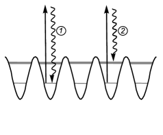
Figure 2: Sketch of the different heating processes in a lattice in the tight-binding limit: intraband processes (1) and interband processes (2).

We now consider the increase rate of energy within the ground band of the optical lattice. For experiments with atomic gases, the physical motivation to do so is twofold: One can imagine observable quantities that depend mainly on the probability amplitudes to find the atoms in the Bloch states of the ground band, and one can also imagine that evaporative-type experimental techniques are developed to continuously eliminate the atoms from the excited energy bands.

Having previously bounded the effect of the light shift correction $\delta U$, we directly neglect it in the master equation Eq. (15), and we define the ground band mean energy as

$$E_{\rm GB}=\frac{\mbox{Tr}[P_{\rm GB}(\frac{\mathbf{p}^{2}}{2m}+U)\bar{\sigma}_{gg}^{\rm diag}]}{\mbox{Tr}[P_{\rm GB}\bar{\sigma}_{gg}^{\rm diag}]}$$ (27)

where $P_{\rm BG}$ projects onto the ground energy band in the periodic potential $U$. The increase rate of $E_{\rm GB}$, contrarily to the total energy increase rate, depends on the atomic state. To make the analytical calculation tractable , we thus restrict to the initial increase rate $\frac{d}{dt}E_{\rm GB}(t=0)$ for an initial atomic state only populating the ground Bloch state, that is the state with zero Bloch vector $\mathbf{q}=\mathbf{0}$ in the ground band (of band indices $\mathbf{0}$). This choice is motivated by the fact that the heating rate of Trotzky et al. (2009) was measured for a Bose-Einstein condensate.

We shall present numerical results in the general case, and then focus on the tight-binding limit, with a modulation depth of the optical potential $U(\mathbf{r})$ much larger than the atomic recoil energy, where analytical results are obtained. It is then convenient to assume that the optical lattice potential has a minimum at the origin $\mathbf{r}=\mathbf{0}$ of the coordinates. We thus take $\mathcal{E}_{\mu}=\mathcal{E}_{0,\mu}\cos(\mathbf{k}_{\mu}\cdot\mathbf{r})$ for a red detuned lattice ($\delta_{J}<0$ $\forall{J}$), and $\mathcal{E}_{\mu}=\mathcal{E}_{0,\mu}\sin(\mathbf{k}_{\mu}\cdot\mathbf{r})$ for a blue detuned lattice ($\delta_{J}>0$ $\forall{J}$).

General results: The initial atomic density operator is:

$$\bar{\sigma}_{gg}^{\rm diag}(t=0)=|\mathbf{0};\mathbf{q}=\mathbf{0}\rangle\langle\mathbf{0};\mathbf{q}=\mathbf{0}|\otimes\sigma_{gg}^{\rm int}.$$ (28)

Here $\sigma_{gg}^{\rm int}$ is any ground internal atomic state (with no hyperfine coherences), $|\mathbf{0};\mathbf{q}\rangle$ is the ground band eigenstate of Bloch vector $\mathbf{q}$, normalized in an arbitrarily large quantization volume commensurate with the lattice spacing, and (for futur reference) $E_{\mathbf{0};\mathbf{q}}$ is the corresponding eigenenergy. Since $\bar{\sigma}_{gg}^{\rm diag}(t=0)$ commutes with $H_{0}=\mathbf{p}^{2}/(2m)+U(\mathbf{r})$ and with the projector $P_{\rm GB}$, the time derivative of the ground band energy at $t=0$ has, from (15), the simple expression involving the feeding term only:

$$\frac{dE_{\rm GB}}{dt}(t=0)=\mbox{Tr}[P_{\rm GB}(H_{0}-E_{\mathbf{0};\mathbf{q}=\mathbf{0}})\mathcal{L}[\bar{\sigma}_{ee}(0)].$$ (29)

Replacing the feeding operator by (18) and the excited state density operator by its expression (19), we obtain at time $t=0$:

$$\frac{dE_{\rm GB}}{dt}=\Gamma\left(\sum_{J}\frac{d_{J}^{2}}{(\hbar\delta_{J})^{2}}\right)\int\frac{d^{2}n}{4\pi}\sum_{\mu}\left[1+\left(\frac{1}{3}-n_{\mu}^{2}\right)C\right]\\ \times(E_{\mathbf{0};k_{L}(\mathbf{e}_{\mu}-\mathbf{n})}-E_{\mathbf{0};\mathbf{0}})|\langle\mathbf{0};k_{L}(\mathbf{e}_{\mu}-\mathbf{n})|e^{-ik_{L}\mathbf{n}\cdot\mathbf{r}}\mathcal{E}_{\mu}(\mathbf{r})|\mathbf{0};\mathbf{0}\rangle|^{2}.$$ (30)

We have used the fact that, after absorption of a laser photon in the mode $\mathcal{E}_{\mu}$ and spontaneous emission of a photon of wavevector $k_{L}\mathbf{n}$, where $k_{0}$ was identified to $k_{L}$, the initial center of mass atomic state of zero Bloch vector acquires a Bloch vector $\mathbf{q}=k_{L}\mathbf{e}_{\mu}-k_{L}\mathbf{n}$. The quantity $C$ results from the evaluation of the trace over the internal atomic variables performed in the decoupled basis, where the dipole operator $\mathcal{D}$ has simple matrix elements on $1/2\to 1/2$ and $1/2\to 3/2$ transitions. It only depends on the atom-laser detunings $\delta_{J}$:

$$C=\frac{3}{2}\ \frac{1+2\delta_{\frac{3}{2}}/\delta_{\frac{1}{2}}}{2+{\delta_{\frac{3}{2}}^{2}/\delta_{\frac{1}{2}}^{2}}}.$$ (31)

In principle, $C$ can range between $-3/4$ and $3/2$. In the useful case of detunings much larger than the fine structure $\omega_{3/2}-\omega_{1/2}$, one has $\delta_{3/2}\approx\delta_{1/2}$ and $C$ approaches $3/2$.

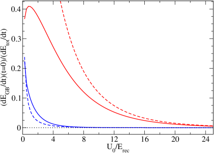
Figure 3: Initial ground band heating rate $dE_{\rm GB}/dt$ for an atom prepared in the ground Bloch state of the optical lattice, for a red lattice (red lines) and for a blue lattice (blue lines), as a function of the lattice depth in recoil units, $U_{0}/E_{\rm rec}$. Here the coefficient $C=3/2$, and the lattice is isotropic: $U_{0,\mu}=U_{0}$ for all spatial directions $\mu=x,y,z$ in Eq.(32) for a red lattice and in Eq.(33) for a blue lattice. Solid lines: Numerical evaluation of (30). Dashed lines: Asymptotic expressions (40) and (42). The ground band heating rate is expressed in units of the total heating rate (25).

The expression (30) allows a straightforward numerical evaluation of the heating rate. It is convenient to introduce the lattice depths $U_{0,\mu}\geq 0$ along each direction $\mu\in\{x,y,z\}$, such that Eq. (16) reads

$$U_{\rm red}(\mathbf{r}) = -P_{g}\sum_{\mu}U_{0,\mu}\cos^{2}k_{L}r_{\mu}$$ (32)

$$U_{\rm blue}(\mathbf{r}) = P_{g}\sum_{\mu}U_{0,\mu}\sin^{2}k_{L}r_{\mu}$$ (33)

for a red detuned and a blue detuned lattice, respectively. In Fig.3, we plot the numerical results for the ground band heating rate in an isotropic lattice $U_{0,\mu}=U_{0}$ $\forall\mu$, either red or blue detuned, in units of the total heating rate (25), as a function of the lattice depth in units of the recoil energy (9), taking $C=3/2$. Whereas the ground band heating rate is of the same order as the total heating rate for shallow lattices $U_{0}\lesssim E_{\rm rec}$, it drops to much smaller values in the tight-binding limit $U_{0}\gg E_{\rm rec}$, the main effect being that the ground band width drops exponentially fast with $(U_{0}/E_{\rm rec})^{1/2}$ in that limit. Furthermore, it is observed in Fig.3 that the ground band heating rate drops faster for a blue detuned lattice than for a red detuned one. This we now explain analytically, not restricting to an isotropic lattice.

Lamb-Dicke regime: We first rewrite the matrix element appearing in (30) in terms of the ground band Wannier function $\Phi_{\mathbf{0}}(\mathbf{r})$, assumed as usual to be real and normalized to unity:

$$\langle\mathbf{0};k_{L}(\mathbf{e}_{\mu}-\mathbf{n})|e^{-ik_{L}\mathbf{n}\cdot\mathbf{r}}\mathcal{E}_{\mu}(\mathbf{r})|\mathbf{0};\mathbf{0}\rangle=\\ \sum_{\mathbf{R}}\int d^{3}r\ \Phi_{\mathbf{0}}(\mathbf{r}-\mathbf{R})e^{-ik_{L}\mathbf{n}\cdot\mathbf{r}}\mathcal{E}_{\mu}(\mathbf{r})\Phi_{0}(\mathbf{r})$$ (34)

where the sum is taken over the locations of the lattice potential minima $\mathbf{R}\in(\pi/k_{L})\mathbb{Z}^{3}$. In the large lattice depth limit $U_{0,\mu}/E_{\rm rec}\gg 1$, the ground band dispersion relation may be approximated by the tight-binding expression

$$E_{\mathbf{0};\mathbf{q}}-E_{\mathbf{0};\mathbf{0}}=\sum_{\nu\in\{x,y,z\}}2t_{\nu}[1-\cos(q_{\nu}\pi/k_{L})].$$ (35)

The sum (34), to zeroth order in the tunneling amplitudes $t_{\nu}\geq 0$, reduces to the $\mathbf{R}=\mathbf{0}$ term. This term may be evaluated by a Lamb-Dicke expansion in powers of $k_{L}a_{\mu}$, resulting from series expansions in powers of $k_{L}r$, e.g.

$$e^{-ik_{L}\mathbf{n}\cdot\mathbf{r}}=1-ik_{L}\mathbf{n}\cdot\mathbf{r}+O(k_{L}r)^{2}.$$ (36)

We have introduced the size

$$a_{\mu}=\left(\frac{\hbar}{2m\omega_{\mu}}\right)^{1/2}=\frac{1}{k_{L}}\left(\frac{E_{\rm rec}}{4U_{0,\mu}}\right)^{1/4}$$ (37)

of the ground state of the harmonic oscillator of angular oscillation frequency $\omega_{\mu}$ that approximates $U(\mathbf{r})$ around $\mathbf{r}=\mathbf{0}$ along direction $\mu$. Restricting to leading order in the Lamb-Dicke expansion, we can also approximate $\Phi_{0}$ with the Gaussian wavefunction of the harmonic oscillator ground state.

Atom	Wavelength $\lambda_{L}$	$E_{\rm rec}$	$\left(\frac{dE_{\rm tot}}{dt}\right)/t_{\nu}$	$\left(\frac{dE_{\rm GB}}{dt}\right)/t_{\nu}$	Ref.
87Rb	$850$ nm	$3.2~{}$kHz	$6~{}$s-1	$1~{}$s-1	Greiner et al. (2002)
87Rb	$750$ nm	$4.1~{}$kHz	$12~{}$s-1	$2\times 10^{-2}~{}$s-1
133Cs	$1064$ nm	$1.3~{}$kHz	$1~{}$s-1	$0.1~{}$s-1	Gemelke et al. (2009)
133Cs	$780$ nm	$2.5~{}$kHz	$2~{}$s-1	$5\times 10^{-3}~{}$s-1
87Rb	x axis: $765$ nm	$3.9~{}$kHz	$8~{}$s-1	$10^{-2}~{}$s-1
	y+z axis:$844$ nm	$2.5~{}$kHz	$2~{}$s-1	$0.3~{}$s-1
	Total:		$10~{}$s-1	$0.3~{}$s-1	Trotzky et al. (2009)

Table 1: Total and ground band heating rates for two different experiments with ⁸⁷Rb and ¹³³Cs, for blue and red detuned isotropic optical lattices of depth per axis $U_{0,\mu}=10~{}E_{\rm R}$. The heating rates are estimated using the formulas (40) and (42) obtained in the Lamb-Dicke limit, and normalized by the ground band tunnel energy $t_{\nu}\approx 2\times 10^{-2}E_{\rm R}$ defined in (35). For these parameters, the coefficient $C$ in Eq. (31) is within $10~{}$% of the asymptotic value $3/2$. The corrections to the light shift potential $U$ discussed in subsection II.3 are very small, $\delta U_{\rm hf}\sim 10^{-4}-10^{-5}$, $\delta U_{\rm micro}\sim 10^{-6}-10^{-7}$, $\delta U_{\rm 1/\delta^{2}}\sim 10^{-3}$. The last two lines refer to the bichromatic lattice of Trotzky et al. (2009).

Red lattice: We use the expansion $\mathcal{E}_{\mu}(\mathbf{r})=\mathcal{E}_{0,\mu}+O(k_{L}r_{\mu})^{2}$ so that

$$\langle\mathbf{0};k_{L}(\mathbf{e}_{\mu}-\mathbf{n})|e^{-ik_{L}\mathbf{n}\cdot\mathbf{r}}\mathcal{E}_{\mu}(\mathbf{r})|\mathbf{0};\mathbf{0}\rangle=\mathcal{E}_{0,\mu}[1+O(k_{L}a_{\rm ho})^{2}],$$ (38)

where $a_{\rm ho}$ is the largest of the $a_{\nu}$. Upon insertion in (30), we face angular integrals that can be calculated in spherical coordinates of axis $\nu$, e.g.

$$\int\frac{d^{2}n}{4\pi}n_{\nu}^{2}\cos(\pi n_{\nu})=\int_{-1}^{1}\frac{du}{2}u^{2}\cos(\pi u)=-\frac{2}{\pi^{2}}.$$ (39)

We obtain the deep lattice asymptotic expression at time $t=0$:

$$\frac{d}{dt}E_{\rm GB}^{\rm red}=\Gamma\left(\sum_{J}\frac{d_{J}^{2}}{(\hbar\delta_{J})^{2}}\right)\sum_{\mu,\nu}2t_{\nu}|\mathcal{E}_{0,\mu}|^{2}\\ \times\left[1+\frac{C}{\pi^{2}}(1+\delta_{\mu\nu})\right],$$ (40)

where $\delta_{\mu\nu}$ is the Kronecker symbol. Expression (40) asymptotically matches the numerical results, see Fig.3. We thus find that, for a red detuned lattice, the ground band heating rate is smaller than the total heating rate by a factor scaling as the tunneling amplitude over the recoil energy. This reduction factor simply originates from the energy width of the ground band.

Blue lattice: The laser field amplitudes vanish in $\mathbf{r}=\mathbf{0}$ and have the expansion $\mathcal{E}_{\mu}(\mathbf{r})=\mathcal{E}_{0,\mu}k_{L}r_{\mu}+O(k_{L}r_{\mu})^{3}$ so that

$$\langle\mathbf{0};k_{L}(\mathbf{e}_{\mu}-\mathbf{n})|e^{-ik_{L}\mathbf{n}\cdot\mathbf{r}}\mathcal{E}_{\mu}(\mathbf{r})|\mathbf{0};\mathbf{0}\rangle=\\ \mathcal{E}_{0,\mu}[-i(k_{L}a_{\mu})^{2}+O(k_{L}a_{\rm ho})^{4}].$$ (41)

Insertion in (30) and angular integration give at time $t=0$:

$$\frac{d}{dt}E_{\rm GB}^{\rm blue}=\Gamma\left(\sum_{J}\frac{d_{J}^{2}}{(\hbar\delta_{J})^{2}}\right)\sum_{\mu,\nu}2t_{\nu}|\mathcal{E}_{0,\mu}|^{2}(k_{L}a_{\mu})^{4}\\ \times\left\{\left(1+\frac{C}{3}\right)\left(\frac{1}{3}-\frac{1}{\pi^{2}}\right)-\left(\frac{1}{5}-\frac{9}{\pi^{4}}\right)C\right.\\ \left.-\delta_{\mu\nu}\left[\frac{1}{\pi^{2}}+\left(\frac{33}{\pi^{4}}-\frac{11}{3\pi^{2}}\right)C\right]\right\}.$$ (42)

This can be further simplified, since $|\mathcal{E}_{0,\mu}|^{2}a_{\mu}^{4}$ is actually independent on the amplitude of the standing wave $\mathcal{E}_{\mu}$ and hence on the direction of space. Expression (42) asymptotically matches the numerical results, see Fig.3. We thus find that the blue detuned lattice has a ground band heating rate that is reduced as compared to the red one (42) by factors $(k_{L}a_{\mu})^{4}\propto E_{\rm rec}/U_{0,\mu}\ll 1$. The first factor $(k_{L}a_{\mu})^{2}$ originates from the reduction of the fluorescence rate as compared to the red lattice, due to the Lamb-Dicke effect: Absorption of a laser photon in the standing wave $\mathcal{E}_{0,\mu}\sin k_{L}r_{\mu}$ brings the atom mainly in the first excited band, with a small transition amplitude $\propto k_{L}a_{\mu}$ leading to a reduced fluorescence rate $\propto(k_{L}a_{\mu})^{2}$. The second factor $(k_{L}a_{\mu})^{2}$ originates from the branching ratio of spontaneous emission from the internal state $e$ in the first excited band to the internal state $g$ in the ground band.

Limits of validity: The ground band energy increases linearly in time (with the rate that we have calculated) only for short times. We can estimate the onset of non-linearity by considering double fluorescence cycles (with the atom arriving in the ground band after the second cycle). For a red detuned (respectively blue detuned) lattice, the probability of such a double cycle over the time interval $t$ is $\propto(\Gamma_{\rm fluo}^{\rm max}t)^{2}$ [respectively $\propto(\Gamma_{\rm fluo}^{\rm max}t)^{2}(k_{L}a_{\rm ho})^{4}$], corresponding to a ground band energy increase $\propto t_{\nu}$. The corresponding mean increase of energy is negligible as compared to the single cycle contribution $\Gamma_{\rm fluo}^{\rm max}tt_{\nu}$ [respectively $\Gamma_{\rm fluo}^{\rm max}tt_{\nu}(k_{L}a_{\rm ho})^{4}$] as long as $\Gamma_{\rm fluo}^{\rm max}t\ll 1$ in both cases.

As a final remark, we point out that the ground band heating rate for a blue lattice, being much smaller in the tight binding limit than the one for a red lattice with the same depth $U_{0}/E_{\rm rec}$, is thus much more sensitive to any additional heating effects not included in our theoretical model, in particular to collisions between ground band and excited band atoms in the many-body case.

V Conclusion

We have performed a full quantum calculation of single atom heating rates in a far-detuned, three-dimensional optical lattice, including explicitly a realistic atomic internal structure and the fact that the superimposed laser standing waves have different frequencies, as in real experiments.

First, we have calculated the total heating rate, that is the rate of increase of the total mechanical energy of the atom. Remarkably, we have found a universal expression, independent of the initial internal and external atomic state, and simply equal to the product of the recoil energy $E_{\rm rec}$ and of the maximal fluorescence rate $\Gamma_{\rm fluo}^{\rm max}$ that may be realized in the lattice. The total heating rate is thus independent of the sign of the laser detuning (red or blue).

This general feature is easy to understand in the limiting case of a deep lattice for an atom initially in the ground energy band: The total heating rate is then determined by rare photon scattering events transferring the atom to excited bands at a rate which is independent of the sign of the detuning. In the blue-detuned case, the atom most probably arrives in the first excited band after a scattering event, which increases the energy by the oscillation quantum $\hbar\omega_{\rm osc}$, that is by much more than the recoil energy; this however takes place at a rate $\propto\Gamma_{\rm fluo}^{\rm max}E_{\rm rec}/\hbar\omega_{\rm osc}\ll\Gamma_{\rm fluo}^{\rm max}$ because of the Lamb-Dicke effect. The product of the rate and of the energy change is indeed $\propto\Gamma_{\rm fluo}^{\rm max}E_{\rm rec}$. In the red-detuned case Wolf et al. (2000), the fluorescence rate, of order $\Gamma_{\rm fluo}^{\rm max}$, is much larger; the atom however mainly returns to the ground band after a scattering event, due to the Lamb-Dicke effect, which increases the energy by much less than the recoil energy; with a branching ratio $\propto E_{\rm rec}/\hbar\omega_{\rm osc}$, the atom however arrives in the first excited band, which increases the energy by $\hbar\omega_{\rm osc}$ and results in a heating rate again $\propto\Gamma_{\rm fluo}^{\rm max}E_{\rm rec}$.

Second, for an atom initially prepared in the lowest Bloch state of the lattice (a minimal single-particle model for the many-body superfluid state realized in experiments), we have calculated the initial ground band heating rate. This is the rate of energy increase due to processes where the atom returns to the ground band of the lattice after a photon scattering event. We have derived analytical expressions of this rate in the deep lattice limit. They show that, in contrast to the total heating rate, the ground band heating rate strongly depends on the laser detuning, and is strongly suppressed for blue detuned lattices: It is of order $\Gamma_{\rm fluo}^{\rm max}t_{0}$ for a red deep lattice, and of order $\Gamma_{\rm fluo}^{\rm max}t_{0}(E_{\rm rec}/\hbar\omega_{\rm osc})^{2}$ for blue deep lattice, where $t_{0}$ is the atomic tunneling amplitude between neighbouring sites.

A recent experiment Trotzky et al. (2009) reported a measured heating rate of $\left(dE/dt\right)_{\rm exp}/t_{0}\approx 3.5{\rm s}^{-1}$, where the tunnelling amplitude $t_{0}$ was essentially independent of the spatial direction. This heating rate was obtained by using Quantum Monte Carlo simulations at several temperatures to calibrate the experimental data: The decrease of the visibility of the interference pattern observed after free expansion was recorded over time, and compared to a “visibility-energy” abacus obtained from the simulations.

The heating rate measured this way is unsurprisingly smaller than the total heating rate that we calculate, see Table 1. Indeed, the Quantum Monte Carlo simulations take into account the ground band only, and we expect the measured interference pattern to depend mostly on the ground band atoms. Hence, the most pertinent rate to compare the experiment to is the ground band heating rate. The measured heating rate is significantly larger than the ground band heating rate, though, see Table 1. To resolve this discrepancy, one would have to include effects that we did not consider in this article: Firstly, heating due to technical noise in the apparatus, which should be quantified for a specific experiment, and secondly, the role of collisions in redistributing part of the energy from the excited to the ground band. To our knowledge, the latter, more fundamental many-body problem, is still quite unexplored Hung et al. (2009) and provides an interesting direction for future work.

We acknowledge useful discussions with I. Bloch, S. Trotzki, L. Pollet, N. Prokof’ev, B. Svistunov, M. Troyer, K. Mur, and J. Dalibard. The authors are members of IFRAF. This work was supported by the DARPA project OLE.

Appendix A Derivation of the ground state master equation

In this Appendix, we provide details about the derivation of the master equation used in the main text. We use an interaction picture with respect to the kinetic plus hyperfine Hamiltonian $H_{0}=\frac{\mathbf{p}^{2}}{2m}+H_{\rm hf}$, where operators are modified as $\tilde{X}(t)=e^{iH_{0}t/\hbar}X(t)e^{-iH_{0}t/\hbar}$. The Bloch equations read

$$\frac{d}{dt}\tilde{\sigma}_{e_{J}g}=(i\delta_{J}-\frac{\Gamma}{2})\tilde{\sigma}_{e_{J}g}\\ +\frac{1}{i\hbar}\Big{[}\left(\tilde{V}_{\rm AL}(t)\right)_{e_{J}g}\tilde{\sigma}_{gg}-\sum_{J^{\prime}}\tilde{\sigma}_{e_{J}e_{J^{\prime}}}\left(\tilde{V}_{\rm AL}(t)\right)_{e_{J^{\prime}}g}\Big{]}$$ (43)

$$\frac{d}{dt}\tilde{\sigma}_{e_{J}e_{J^{\prime}}}=[i(\delta_{J}-\delta_{J^{\prime}})-\Gamma]\tilde{\sigma}_{e_{J}e_{J^{\prime}}}\\ +\frac{1}{i\hbar}\left[\left(\tilde{V}_{\rm AL}(t)\right)_{e_{J}g}\tilde{\sigma}_{ge_{J^{\prime}}}-\tilde{\sigma}_{e_{J}g}\left(\tilde{V}_{\rm AL}(t)\right)_{ge_{J^{\prime}}}\right]$$ (44)

$$\frac{d}{dt}\tilde{\sigma}_{gg}=\tilde{\mathcal{L}}[\tilde{\sigma}_{ee}]+\frac{1}{i\hbar}\sum_{J}\left[\left(\tilde{V}_{\rm AL}(t)\right)_{ge_{J}}\tilde{\sigma}_{e_{J}g}-\mbox{h.c.}\right].$$ (45)

The feeding term of the ground state by spontaneous emission is given in Schrödinger picture by (18).

We perform the series of approximations discussed in the main text. Integrating formally Eq. (43), after omission of $\tilde{\sigma}_{ee}$, neglecting $\mathbf{p}^{2}/2m$ as compared to $\hbar\Gamma$, and neglecting a transient of duration $1/\Gamma$, we obtain the steady state optical coherence

$$\tilde{\sigma}_{e_{J}g}(t)=\int_{0}^{+\infty}\frac{d\tau}{i\hbar}\,e^{(i\delta_{J}-\Gamma/2)\tau}\left(\tilde{V}_{\rm AL}(t-\tau)\right)_{e_{J}g}\tilde{\sigma}_{gg}(t-\tau).$$ (46)

By repeated integrations by parts of the integral over $\tau$, integrating the exponential factor, we get a formal expansion of $\tilde{\sigma}_{e_{J}g}(t)$ in powers of $1/(\delta_{J}+i\Gamma/2)$, that we turn into a series in $1/\delta_{J}$.

To order $1/\delta$: The optical coherences in Schrödinger picture are given by

$$\sigma_{e_{J}g}^{(1)}(t)=\frac{1}{\hbar\delta_{J}}\left(V_{\rm AL}(t)\right)_{e_{J}g}\sigma_{gg}(t).$$ (47)

This is familiar for a constant atom-laser coupling. We have shown that it holds even for a time dependent coupling provided that Eq. (3) holds. Inserting this relation Eq. (47) in Eq. (44) gives in steady state $\sigma_{e_{J}e_{J^{\prime}}}^{(1)}=0$. After insertion of Eq. (47) in Eq. (45) we then find that $\sigma_{gg}^{\rm diag}$ has a purely conservative evolution of Hamiltonian $H_{\rm hf}^{g}+\frac{\mathbf{p}^{2}}{2m}+U^{(1)}(\mathbf{r},t)$ with the time-dependent light shift potential:

$$U^{(1)}(\mathbf{r},t)=\sum_{J}\frac{1}{\hbar\delta_{J}}\left(V_{\rm AL}(t)\right)_{ge_{J}}\left(V_{\rm AL}(t)\right)_{e_{J}g}.$$ (48)

As expected $U^{(1)}/\hbar$ is of order $\Omega^{2}/\delta$ so that $d\tilde{\sigma}_{gg}/dt$ is at most of this order; in general, $U^{(1)}$ can induce Zeeman and even hyperfine ground state coherences

To order $1/\delta^{2}$: From Eq. (46) we obtain

$$\tilde{\sigma}_{e_{J}g}^{(2)}(t)=\frac{-i}{\hbar\delta_{J}^{2}}\left[\frac{\Gamma}{2}+\frac{d}{dt}\right]\left[\left(\tilde{V}_{\rm AL}(t)\right)_{e_{J}g}\tilde{\sigma}_{gg}(t)\right].$$ (49)

We shall neglect $d\tilde{\sigma}_{gg}/dt$ with respect to $\Gamma\tilde{\sigma}_{gg}$ as allowed by Eq. (8). Inserting Eq. (49) in Eq. (45) has two effects. First it induces a small modification of the light shift potential of order Eq. (14):

$$U^{(2)}=\sum_{J}\frac{1}{(\hbar\delta_{{J}})^{2}}\Big{\{}\left(V_{\rm AL}(t)\right)_{ge_{J}}\Big{(}[H_{\rm hf},V_{\rm AL}(t)]\Big{)}_{e_{J}g}\\ -\frac{i\hbar}{2}\Big{[}\left(V_{\rm AL}(t)\right)_{ge_{J}}\left(\frac{d}{dt}V_{\rm AL}(t)\right)_{e_{J}g}-\mbox{h.c.}\Big{]}\Big{\}}.$$ (50)

Second it induces a lossy evolution of $\sigma_{gg}^{\rm diag}$, $\frac{d}{dt}\sigma_{gg}\Big{|}_{\rm loss}=-\frac{1}{2}\{W,\sigma_{gg}\}$, with

$$W^{(2)}=\sum_{J}\frac{1}{(\hbar\delta_{J})^{2}}\left[\Gamma+\frac{d}{dt}\right]\left(V_{\rm AL}(t)\right)_{ge_{J}}\left(V_{\rm AL}(t)\right)_{e_{J}g}.$$ (51)

The adiabatic elimination of the excited state matrix elements up to order $1/\delta^{2}$, remarkably leads to an expression similar to the usual two-level atom case, despite the presence of the hyperfine Hamiltonian $H_{\rm hf}^{e_{J}}$ and the time dependence of $V_{\rm AL}$:

$$\sigma_{e_{J}e_{J^{\prime}}}^{(2)}=\frac{\left(V_{\rm AL}(t)\right)_{e_{J}g}\sigma_{gg}^{\rm diag}\left(V_{\rm AL}(t)\right)_{ge_{J^{\prime}}}}{\hbar^{2}\delta_{J}\delta_{J^{\prime}}}+O\left[\left(\frac{\Omega}{\delta}\right)^{2}\frac{\Omega^{2}}{\delta\Gamma}\right].$$ (52)

This may me checked by direct insertion of Eq. (49) in Eq. (44), the $O[\ldots]$ term coming from neglecting $d\tilde{\sigma}_{gg}/dt$ as allowed by Eq. (8). When inserted in Eq. (45) this provides a closed equation for $\sigma_{gg}^{\rm diag}$.

Temporal average: Under the conditions discussed in the main text, we now average out the rapidly oscillating terms in the ground state master equation. The lattice potential $U^{(1)}(\mathbf{r},t)$ to order $1/\delta$ contains a zero frequency part, which is scalar according to Eq. (5) and is called $U$ in Eq. (16). It also contains oscillating contributions $U^{(1)}_{\mu\nu}(\mathbf{r})e^{-i\Delta_{\mu\nu}t}$, with $\Delta_{\mu\nu}=\Delta_{\mu}-\Delta_{\nu}\neq 0$, $\mu\neq\nu$, supposed to be pairwise distinct, as it is the case in Trotzky et al. (2009), and

$$U_{\mu\nu}^{(1)}(\mathbf{r})=\sum_{J}\frac{(D_{\nu})_{ge_{J}}\mathcal{E}^{*}_{\nu}(\mathbf{r})(D_{\mu})_{e_{J}g}\mathcal{E}_{\mu}(\mathbf{r})}{\hbar\delta_{J}}$$ (53)

These contributions are in general not scalar. It is convenient to split $U_{\mu\nu}^{(1)}$ in (i) an off-diagonal part, inducing coherences between the two hyperfine ground states, that is a raising (resp. lowering) part $(U_{\mu\nu}^{(1)})_{\pm}$ coupling $g_{1}$ to $g_{2}$ (resp. $g_{2}$ to $g_{1}$), and (ii) a diagonal part $(U_{\mu\nu}^{(1)})_{\rm diag}$ coupling $g_{1}$ to $g_{1}$ and $g_{2}$ to $g_{2}$. In the interaction picture, the diagonal parts correspond to terms modulated at frequencies $\Delta_{\mu\nu}$ in $\tilde{U}^{(1)}$, and the off-diagonal parts to terms modulated at frequencies $\Delta_{\mu\nu}\mp\Delta_{\rm hf}^{g}$. They will induce rapidly oscillating components of the density operator $\tilde{\sigma}_{gg}$ at those frequencies, these components being very small here since $\hbar\Omega^{2}/\delta\ll|\Delta_{\mu\nu}|,\Delta_{\rm hf}^{g}$. In the present regime $\Delta_{\rm hf}^{g}\gg\Delta_{\rm mod}$, we can treat separately the effect of the off-diagonal and diagonal parts of $U^{(1)}$.

The off-diagonal part of $U^{(1)}(t)$ induces a Rabi coupling $\approx\hbar\Omega^{2}/\delta$ between $g_{1}$ and $g_{2}$ much smaller than their energy splitting $\hbar\Delta_{\rm hf}^{g}$, with a very slow time variation at the scale of $1/\Delta_{\rm hf}^{g}$. Hence we treat it directly to second order in usual perturbation theory for a fixed time $t$ and then average the result over time. This leads to an effective light shift potential acting within each hyperfine ground state:

$$U_{\rm eff,I}^{(1)}=-\sum_{\mu\neq\nu}\frac{(U_{\nu\mu}^{(1)})_{-}(U_{\mu\nu}^{(1)})_{+}-(U_{\nu\mu}^{(1)})_{+}(U_{\mu\nu}^{(1)})_{-}}{\hbar\Delta_{\rm hf}^{g}}.$$ (54)

This corresponds to Eq. (11) with a different notation. Having eliminated the hyperfine coherences, we consider in what follows $\bar{\sigma}_{gg}^{\rm diag}$.

The diagonal part of $U^{(1)}_{\mu\nu}$ couples the zero frequency component $\bar{\sigma}_{gg}^{\rm diag}$ to rapidly modulated components $\sigma_{gg}^{\mu\nu}(t)e^{-i\Delta_{\mu\nu}t}$; adiabatic elimination gives the slowly evolving amplitudes

$$\sigma_{gg}^{\mu\nu}(t)=\frac{[(U^{(1)}_{\mu\nu})_{\rm diag},\bar{\sigma}_{gg}^{\rm diag}]}{\hbar\Delta_{\mu\nu}}.$$ (55)

They are small according to Eq. (10). Including the coupling of $\bar{\sigma}_{gg}^{\rm diag}$ to $\sigma_{gg}^{\nu\mu}$ by $(U_{\mu\nu}^{(1)})_{\rm diag}$ gives the a priori leading contribution to the effective potential induced by the diagonal micromotion:

$$U_{\rm eff,II}^{(1)}=\sum_{\mu\neq\nu}\frac{[(U_{\mu\nu}^{(1)})_{\rm diag}^{\dagger},(U_{\mu\nu}^{(1)})_{\rm diag}]}{2\hbar\Delta_{\mu\nu}}+\ldots$$ (56)

Usually, the micromotion is studied for a spinless particle, in which case the commutator in Eq. (56) automatically vanishes and the first non-zero correction scales as $1/\Delta_{\rm mod}^{2}$ Rahav et al. (2003); Ridinger and Weiss (2009). Here, the atom has a non-zero spin. From a calculation in the decoupled basis we find Cohen-Tannoudji and Dupont-Roc (1972) $U_{\mu\nu}^{(1)}=\mathcal{E}_{\mu}\mathcal{E}_{\nu}^{*}(2id^{2}/3\hbar^{2})\,\mathbf{J}\cdot(\mathbf{e}_{\mu}\times\mathbf{e}_{\nu})[\delta_{3/2}^{-1}-\delta_{1/2}^{-1}]$. The commutator in Eq. (56) thus vanishes also in our spinorial case for the field Eq. (1). Going to next order in $1/\Delta_{\rm mod}$ with the formalism of Rahav et al. (2003) extended to the case with a spin we finally find a non-zero contribution

$$U_{\rm eff,II}^{(1)}=\sum_{\mu\neq\nu}\frac{\mbox{\small grad}\,(U_{\mu\nu}^{(1)})_{\rm diag}^{\dagger}\cdot\mbox{\small grad}\,(U_{\mu\nu}^{(1)})_{\rm diag}}{2m\Delta_{\mu\nu}^{2}}.$$ (57)

This corresponds to Eq. (13) with a different notation. In appendix B we present an alternative derivation of this result, based on the dressed atom approach, and showing that there is no other micromotion term of order $1/\Delta_{\rm mod}^{2}$. Summing both contributions Eqs.(54,57), we get the effective time-independent correction to the light shift potential for the theory of order $1/\delta$, integrating out the effect of hyperfine couplings and diagonal atomic micromotions.

To eliminate the rapidly varying temporal components in the $1/\delta^{2}$ terms of $d\sigma_{gg}/dt$, we simply take the temporal averages, neglecting micromotion corrections at this order, as allowed in particular by Eq. (8). We also project out the operators inducing ground state hyperfine coherences. The $1/\delta^{2}$ correction $\bar{U}^{(2)}_{\rm diag}$ to the light shift is obtained by projecting out the hyperfine coherences of Eq. (50) and taking the temporal average. Its explicit expression is not required here. The complete expression for $\delta U$ in Eq. (15) is

$$\delta U\equiv U^{(1)}_{\rm eff,I}+U^{(1)}_{\rm eff,II}+\bar{U}^{(2)}_{\rm diag}.$$ (58)

The time average of Eq. (51) and the use of the scalarity relation Eq. (5) gives the lossy part of Eq. (15). The time average of Eq. (52) gives Eq. (19) with a different notation.

Appendix B A derivation of the micromotion potential based on the dressed atom picture

We propose here a derivation of the micromotion potential alternative to Rahav et al. (2003) and including the atomic spin. The idea is to use the dressed atom approach Cohen-Tannoudji et al. (1992) to eliminate the time-dependence of the Hamiltonian, and to use standard time-independent effective Hamiltonian theory Cohen-Tannoudji et al. (1992). The laser field is then assumed to be initially in a Fock state with huge occupation numbers $n_{\mu}$ in each mode $\mathcal{E}_{\mu}$ of frequency $\omega_{L}+\Delta_{\mu}$. One may then neglect the dependence of the atom-laser coupling with the photon number, replacing there the photon annihilation operators $a_{\mu}$ with $n_{\mu}^{1/2}A_{\mu}$, where the phase operator $A_{\mu}=(a_{\mu}a_{\mu}^{\dagger})^{-1/2}a_{\mu}$ has unit matrix elements in the Fock basis Carruthers and Nieto (1968). The resulting Hamiltonian is $H=H_{0}+V$ with

$$H_{0} = h_{0}+\sum_{\mu}\hbar(\omega_{L}+\Delta_{\mu})(a_{\mu}^{\dagger}a_{\mu}-n_{\mu})$$ (59)

$$V = \sum_{\mu\neq\nu}\left(U^{(1)}_{\mu\nu}\right)_{\rm diag}A_{\nu}^{\dagger}A_{\mu}$$ (60)

where $h_{0}=\frac{\mathbf{p}^{2}}{2m}+\bar{U}$ is a purely atomic Hamiltonian, $U^{(1)}_{\mu\nu}$ is given by (53) and $\bar{U}$ is the time independent part of $U^{(1)}$, called $U$ in (16). It is convenient to set $(U^{(1)}_{\mu\nu})_{\rm diag}=\mathcal{E}_{\nu}^{*}\mathcal{E}_{\mu}T_{\mu\nu}$ where the operator $T_{\mu\nu}$ does not depend on the atomic position and obeys

$$T_{\mu\nu}^{\dagger}=-T_{\mu\nu}=T_{\nu\mu}.$$ (61)

Since the field is initially in the Fock state $|(n_{\mu})_{\mu\in\{x,y,z\}}\rangle$, we introduce the orthogonal projector $P$ on that Fock state, and $Q=1-P$ the supplementary projector. The effective Hamiltonian $H_{\rm eff}(E)$ inside the subspace over which $P$ projects is exactly given by

$$H_{\rm eff}(E)=h_{0}P+PVQ\frac{Q}{EQ-QHQ}QVP,$$ (62)

where we used $PVP=0$ resulting from the fact that $V$ does not conserve the number of photons in each mode. At this stage, $E$ is arbitrary but much smaller than $\hbar\Delta_{\rm mod}$. Since the denominator in (62) is of order $\hbar\Delta_{\rm mod}\gg V$, because of the occurrence of the projector $Q$, we may expand (62) in powers of $V$, restricting to terms of order up to $1/\Delta_{\rm mod}^{2}$:

$$H_{\rm eff}(E)=h_{0}P+PVQ\frac{Q}{EQ-QH_{0}Q}QVP\\ +PVQ\frac{Q}{EQ-QH_{0}Q}QVQ\frac{Q}{EQ-QH_{0}Q}QVP\\ +O(1/\Delta_{\rm mod}^{3}).$$ (63)

We first focus on the terms of order $V^{3}$ in (63). In the denominators, $\sum_{\mu}\hbar(\omega_{L}+\Delta_{\mu})(a_{\mu}^{\dagger}a_{\mu}-n_{\mu})$ gives contributions of order $\hbar\Delta_{\rm mod}$ that dominate over $E-h_{0}$. Expanding in powers of $(E-h_{0})/\Delta_{\rm mod}$ then gives

$$H_{\rm eff}^{(3)}(E)=\sum^{\prime}_{\alpha,\beta,\gamma}P|\mathcal{E}_{\alpha}|^{2}|\mathcal{E}_{\beta}|^{2}|\mathcal{E}_{\gamma}|^{2}\left(\frac{T_{\alpha\beta}T_{\gamma\alpha}T_{\beta\gamma}}{\hbar^{2}\Delta_{\alpha\beta}\Delta_{\gamma\beta}}\right.\\ +\left.\frac{T_{\alpha\beta}T_{\beta\gamma}T_{\gamma\alpha}}{\hbar^{2}\Delta_{\alpha\beta}\Delta_{\alpha\gamma}}\right)P+O(1/\Delta_{\rm mod}^{3}),$$ (64)

where we recall that $\Delta_{\mu\nu}=\Delta_{\mu}-\Delta_{\nu}$, and the prime on $\sum$ means that the sum is taken over indices that are pairwise distinct. Since the modulation frequencies $\Delta_{\mu}$ are incommensurate, a first action of $V$ on the Fock state $|(n_{\mu})\rangle$, e.g. creating a photon in mode $\alpha$ and annihilating a photon in mode $\beta$, has to be compensated in two steps, either annihilating $\alpha$ in the first step and creating $\beta$ in the second step, or vice-versa, hence the occurrence of two terms in (64). Exchanging the summation indices $\alpha$ and $\beta$ in the second term of (64), and using the antisymmetry of $T_{\alpha\beta}$ and $\Delta_{\alpha\beta}$ under the exchange $\alpha\leftrightarrow\beta$, a sum $1/\Delta_{\beta\gamma}+1/\Delta_{\gamma\beta}=0$ appears, so that

$$H_{\rm eff}^{(3)}(E)=O(1/\Delta_{\rm mod}^{3}),$$ (65)

and may be neglected.

We are left with the $V^{2}$ contribution to $H_{\rm eff}$:

$$H_{\rm eff}^{(2)}(E)=\sum_{\mu\neq\nu}P(U^{(1)}_{\mu\nu})_{\rm diag}\frac{1}{E-h_{0}-\hbar\Delta_{\mu\nu}}(U^{(1)}_{\nu\mu})_{\rm diag}P.$$ (66)

We expand this expression up to order $1/\Delta_{\rm mod}^{2}$:

$$H_{\rm eff}^{(2)}(E)=\sum_{\mu\neq\nu}P|\mathcal{E}_{\mu}|^{2}|\mathcal{E}_{\nu}|^{2}T_{\mu\nu}\frac{1}{-\hbar\Delta_{\mu\nu}}T_{\nu\mu}P\\ +\sum_{\mu\neq\nu}P(U^{(1)}_{\mu\nu})_{\rm diag}(h_{0}-E)(U^{(1)}_{\nu\mu})_{\rm diag}P\frac{1}{(\hbar\Delta_{\mu\nu})^{2}}\\ +O(1/\Delta_{\rm mod}^{3}).$$ (67)

The first contribution, of order $1/\Delta_{\rm mod}$, corresponds to the effective potential given in (56) and vanishes, as already noted in Appendix A, since $T_{\mu\nu}$ and $\Delta_{\mu\nu}$ are antisymmetric functions of $\mu$ and $\nu$. The second contribution does not vanish. Since it is of order $1/\Delta_{\rm mod}^{2}$ already, we treat it in perturbation theory: An unperturbed eigenstate $|\lambda_{0}\rangle$ of $h_{0}$ of energy $E_{0}$ experiences an energy shift, calculated here up to order $(V/\Delta_{\rm mod})^{2}$, equal to

$$E_{2}=\langle\lambda_{0}|H_{\rm eff}^{(2)}(E_{0})|\lambda_{0}\rangle.$$ (68)

Taking advantage of the fact that $\Delta_{\mu\nu}^{2}=\Delta_{\nu\mu}^{2}$, we use the relation

$$\langle\lambda_{0}|(U^{(1)}_{\mu\nu})_{\rm diag}(h_{0}-E_{0})(U^{(1)}_{\nu\mu})_{\rm diag}|\lambda_{0}\rangle+\mu\leftrightarrow\nu=\\ \langle\lambda_{0}|[[(U^{(1)}_{\mu\nu})_{\rm diag},h_{0}],(U^{(1)}_{\nu\mu})_{\rm diag}]|\lambda_{0}\rangle.$$ (69)

Since $\bar{U}$ is scalar, it commutes with $(U^{(1)}_{\mu\nu})_{\rm diag}$ and the kinetic energy operator $\mathbf{p}^{2}/(2m)$ is the only one to contribute to the commutator. After an explicit calculation of the double commutator, we obtain

$$E_{2}=\langle\lambda_{0}|U^{(1)}_{\rm eff,II}(\mathbf{r})|\lambda_{0}\rangle$$ (70)

where $U^{(1)}_{\rm eff,II}(\mathbf{r})$ is indeed given by (57).

References

• Bloch et al. (2008) I. Bloch, J. Dalibard, and W. Zwerger, Rev. Mod. Phys. 80, 885 (2008).
• Mandel et al. (2003) O. Mandel, M. Greiner, A. Widera, T. Rom, T. W. Hänsch, and I. Bloch, Nature 425, 937 (2003).
• Trotzky et al. (2009) S. Trotzky, L. Pollet, F. Gerbier, U. Schnorrberger, I. Bloch, N. Prokof’ev, B. Svistunov, and M. Troyer, arXiv:0905.4882 (2009).
• Gordon and Ashkin (1980) J. P. Gordon and A. Ashkin, Phys. Rev. A 21, 1606 (1980).
• Cook (1980) R. J. Cook, Phys. Rev. Lett. 44, 976 (1980).
• Kazantsev et al. (1981) A. Kazantsev, G. Surdutovich, and V. Yakovlev, J. Physique 42, 1231 (1981).
• Dalibard and Cohen-Tannoudji (1985) J. Dalibard and C. Cohen-Tannoudji, J. Physics B 18, 1661 (1985).
• Berg-Sørensen et al. (1992) K. Berg-Sørensen, Y. Castin, E. Bonderup, and K. Mølmer, J. Phys. B 25, 4195 (1992).
• Castin et al. (1994) Y. Castin, K. Berg-Sørensen, J. Dalibard, and K. Mølmer, Phys. Rev. A 50, 5092 (1994).
• Wineland and Itano (1979) D. J. Wineland and W. M. Itano, Phys. Rev. A 20, 1521 (1979).
• Cirac et al. (1992) J. I. Cirac, R. Blatt, P. Zoller, and W. D. Phillips, Phys. Rev. A 46, 2668 (1992).
• Castin and Dalibard (1991) Y. Castin and J. Dalibard, Europhys. Lett. 14, 761 (1991).
• Berg-Sørensen et al. (1993) K. Berg-Sørensen, Y. Castin, K. Mølmer, and J. Dalibard, Europhys. Lett. 22, 663 (1993).
• Xu et al. (2005) K. Xu, Y. Liu, J. R. Abo-Shaeer, T. Mukaiyama, J. K. Chin, D. E. Miller, W. Ketterle, K. M. Jones, and E. Tiesinga, Phys. Rev. A 72, 043604 (2005).
• Cirac et al. (1996) J. Cirac, M. Lewenstein, and P. Zoller, Europhys. Lett. 35, 647 (1996).
• Castin et al. (1998) Y. Castin, J. I. Cirac, and M. Lewenstein, Phys. Rev. Lett. 80, 5305 (1998).
• Wolf et al. (2000) S. Wolf, S. J. Oliver, and D. S. Weiss, Phys. Rev. Lett. 85, 4249 (2000).
• Cohen-Tannoudji (1992) C. Cohen-Tannoudji, in Fundamental Systems in Quantum Optics, Les Houches Session LIII, edited by J. Dalibard, J. Raimond, and J. Zinn-Justin (Elsevier Science Publisher B.V, 1992), p. 1.
• Paul (1990) W. Paul, Rev. Mod. Phys. 62, 531 (1990).
• Rahav et al. (2003) S. Rahav, I. Gilary, and S. Fishman, Phys. Rev. Lett. 91, 110404 (2003).
• Ridinger and Weiss (2009) A. Ridinger and C. Weiss, Phys. Rev. A 79, 013414 (2009).
• Greiner et al. (2002) M. Greiner, O. Mandel, T. Esslinger, T. W. Hänsch, and I. Bloch, Nature 415, 39 (2002).
• Gemelke et al. (2009) N. Gemelke, X. Zhang, C.-L. Hung, and C. Chin, Nature 460, 995 (2009).
• Hung et al. (2009) C.-L. Hung, X. Zhang, N. Gemelke, and C. Chin, preprint arXiv:0910.1382 (2009).
• Cohen-Tannoudji and Dupont-Roc (1972) C. Cohen-Tannoudji and J. Dupont-Roc, Phys. Rev. A 5, 968 (1972).
• Cohen-Tannoudji et al. (1992) C. Cohen-Tannoudji, J. Dupont-Roc, and G. Grynberg, Atom-Photon Interactions (Wiley, New York, 1992).
• Carruthers and Nieto (1968) P. Carruthers and M. Nieto, Rev. Mod. Phys. 40, 411 (1968).
• Castin and Mølmer (1995) Y. Castin and K. Mølmer, Phys. Rev. Lett. 74, 3772 (1995).