ABSTRACT In this paper, we introduce an approach to the protein folding problem from the point of view of statistical physics. Protein folding is a stochastic process by which a polypeptide folds into its characteristic and functional 3D structure from random coil. The process involves an intricate interplay between global geometry and local structure, and each protein seems to present special problems. The first part of this chapter contains a concise discussion on kinetics versus thermodynamics in protein folding, and introduce the statistical physics basis of protein folding. In the second part, we introduce CSAW (conditioned self-avoiding walk), a model of protein folding that combines the features of self-avoiding walk (SAW) and the Monte Carlo method. In this model, the unfolded protein chain is treated as a random coil described by SAW. Folding is induced by hydrophobic forces and other interactions, such as hydrogen bonding, which can be taken into account by imposing conditions on SAW. Conceptually, the mathematical basis is a generalized Langevin equation. Despite the simplicity, the model provides clues to study the universal aspects while we overlook details and concentrate only on a few general properties. To illustrate the flexibility and capabilities of the model, we consider several examples, including helix formation, elastic properties, and the transition in the folding of myoglobin. From the CSAW simulation and physical arguments, we find a universal elastic energy for proteins, which depends only on the radius of gyration $R_{g}$ and the residue number $N$. The elastic energy gives rise to scaling laws $R_{g}\sim N^{\nu}$ in different regions with exponents $\nu=3/5,3/7,2/5$, consistent with the observed unfolded stage, pre-globule, and molten globule, respectively. These results indicate that CSAW can serve as a theoretical laboratory to study universal principles in protein folding.

1 Introduction

In spite of considerable efforts in the past decades, the protein folding problem is still unsolved and remains one of the most basic intellectual challenges in molecular biology (Branden & Tooze,, 1998; Shakhnovich,, 2006; Zhang,, 2008). The principle through which the amino acid sequence determines the native structure, as well as the dynamics of the process, remain open questions.

In the past 36 years, thinking in the protein folding field has being strongly influenced by Christian Anfinsen’s “thermodynamic hypothesis”. This hypothesis states that the native state of a protein is the one with the lowest Gibbs free energy, and is determined by the totality of interatomic interactions of the amino-acid sequence, in a given environment (Anfinsen,, 1973). Predicting the 3D structure of a protein from its amino-acid sequence is one of the most important goals in the protein folding problem (Moult et al. ,, 1995; Zhang & Skolnick,, 2005; Zhang,, 2008).

Despite this widely established thermodynamic hypothesis (Dill,, 1990; Kim & Baldwin,, 1990), recent experiments have suggested that there may be exceptions, especially for larger and complex proteins (Baker & Agard,, 1994; Baker,, 1998; Lazaridis & Karplus,, 2003; Shakhnovich,, 2006). For these proteins, the native conformations correspond to the kinetically most accessible state (kinetic control), instead of the most stable one (thermodynamic control) (Lazaridis & Karplus,, 2003). This would be the case when the barriers between conformations are too high to be ergodic kinetically, and the protein ends up at a state of local minimum energy that is accessible in available time.

Molecular dynamics (MD) is an invaluable tool with which to study protein folding dynamics in vitro (Day & Daggett,, 2003; Scheraga et al. ,, 2007). MD solves the Newtonian equations of the motion of all atoms in a protein on a computer, using appropriate interatomic potentials. To describe the solvent, one includes thousands of water molecules explicitly, treating all atoms in the water on the same footing as those on the protein chain. For the integration algorithm to be stable, the time step $\Delta t$ must be an order of magnitude smaller than the fastest motions of the system, typically the vibration of a covalent bond, whose period is the order of 10 fs. Thus, the time step is of the order of 1 fs (McCammon et al. ,, 1977; Pearlman et al. ,, 1995). Not surprisingly, such an extravagant use of computing power is so inefficient that one can follow the folding process only to about a microsecond (Duan & Kollman,, 1998; Jang et al. ,, 2003), whereas the folding of a real protein takes from seconds to minutes. The use of reduced models (meso-scopic, coarse-grained, implicit-solvent) with physically based potentials is a reasonable trade-off between computational cost and accuracy (Levitt,, 1976; Kaźmierkiewicz et al. ,, 2002, 2003; Nielsen et al. ,, 2004; Huang,, 2007; Sun,, 2007).

Proteins with different amino acid sequences can invoke quite different folding mechanisms (Daggett & Fersht,, 2003), while proteins with high sequence similarity can end up with very different folds (Alexander et al. ,, 2005; He et al. ,, 2005). Nevertheless, universal aspects do emerge, if one overlooks details and concentrates only on a few general properties. These will be the main subject in this chapter.

We are concerned here with a perspective of protein folding from the point of view of statistical physics (Huang,, 2005). After all, the protein is a chain molecule immersed in water, and, like all physical systems, will tend towards thermodynamic equilibrium with the environment. The process is stochastic, involving an intricate interplay between global geometry and local structure. Our goal is to design a model amenable to computer simulation in a reasonable time, and to investigate the physical principles of protein folding, in particular the relative importance of various interactions.

We treat the protein as a molecular chain performing Brownian motion in water, regarded as a medium exerting random forces on the chain, with the concomitant energy dissipation. In addition, we include regular (non-random) interactions within the chain, as well as between the chain and the medium. Protein folding is a stochastic process of conformation changes, and must be analyzed in terms of a statistical ensemble, but not of a single pathway. In this perspective, we study protein folding by defining a transition probabilities between the conformations, which are described through a Monte Carlo type model.

The unfolded chain is assumed to be a random coil described by SAW (self-avoiding walk), as suggested by Flory some time ago (Flory,, 1953). That is, links in the chain correspond to successive random steps, in which the chain is prohibited from revisiting an occupied position.

We model the protein chain in 3D space, keeping only degrees of freedom relevant to folding, which we take to be the torsional angles between successive links. In a computer simulation, we first generate an ensemble of SAW’s, and then choose a sub-ensemble through a Monte Carlo method, which generates a canonical ensemble with respect to a Hamiltonian that specifies the interactions. We call the model CSAW (conditioned self-avoiding walk) (Huang,, 2007). Mathematically speaking, it is based on a Langevin equation describing the Brownian motion of a chain with interactions. There seems little doubt that such an equation does describe a protein molecule in water, for it is just Newton’s equation with the environment treated as a stochastic medium.

Two types of interactions are included in our initial formulation:

• the hydrophobic interaction with the medium, which causes the chain to fold;

• hydrogen bonding within the chain, which leads to secondary structures.

The model can be implemented efficiently, and is flexible enough to be used as a theoretical laboratory. In our initial studies, we keep only the two interactions listed above, in order to describe the folding dynamics qualitatively. Other interactions, such as electrostatic and van der Waals interactions, can be add as refinements.

Both CSAW and MD are based on Newtonian mechanics, and differ only in the idealization of the system. In CSAW we replace the thousands of water molecules used in MD by a stochastic medium—the heat reservoir of statistical mechanics. With this simplification, we consider the main interactions—hydrophobic interaction and heat dissipation, and ignore inessential degrees of freedom, such as small vibration in the length and angles of the chemical bonds in the protein chain. The advantages of this idealization are that we

• avoid squandering computer power on irrelevant calculations;

• gain a better physical understanding of the folding process.

After a brief review of the basics of protein folding and stochastic processes, we shall describe the model in more detail, and illustrate its use through examples involving realistic protein fragments. We will demonstrate helix formation, elastic properties, and folding stages.

Our results indicate that the CSAW model can describe qualitative features in the folding of simple proteins, and provide physical insight on the mechanisms of protein folding.

2 Protein basics

2.1 The protein chain

The protein is a polypeptide chain consists of a sequence of units or “residues”, which are amino acids chosen from a pool of 20. This sequence is called the primary structure. Along the protein chain, the amino acids are connected by peptide bonds between the C atom of one residue and the nitrogen atom of the next. The center of each amino acid is a carbon called $\mathrm{C}_{\alpha}$. The amino acids differ from each other only in the side chains connected to the $\mathrm{C}_{\alpha}$’s. The side chains can be grouped to different classes by their hydrophobicity, charge, and polarity (Branden & Tooze,, 1998).

A polypeptide chain can also be viewed as repeating peptide units that connect one $\mathrm{C}_{\alpha}$ atom to the next one along the backbone (Figure 1). All atoms in such a unit are fixed in a plane, the peptide plane, with the bond lengths and bond angles very nearly the same in all units in all proteins (Table 1).

Figure 1: Schematic representation of the protein chain. The center of a residue is a carbon atom labeled $\alpha$. The residues are connected by the peptide bonds between the C atom of one residue and the nitrogen atom of the next. All atoms connected to the peptide bond lie on a plane, the peptide plane. The only degrees of freedom we consider are the torsion angles $\phi,\psi$ that specify the relative orientation of successive peptide planes. Residues can differ only in the side chains labeled $R$, chosen from a pool of twenty.

The relative orientation of successive units is determined by the two torsion angles (aka dihedral angle) $\phi$ and $\psi$, as schematically illustrated in Figure 1. The torsion angles $\phi$ and $\psi$ are rotation angles about the $\mathrm{N}$-$\mathrm{C}_{\alpha}$ and $\mathrm{C}_{\alpha}$-$\mathrm{C}$ bonds, respectively, the positive sense being defined according to the right-hand rule. By definition, the flat chain, with all backbone atoms lying in a plane, corresponds to $\phi=\psi=180^{\circ}$ for all residues.

When small vibrations in bond lengths and bond angles are neglected, the torsion angles are the only degrees of freedom. For our purpose, therefore, a protein of $N$ residues has $2(N-1)$ degrees of freedom, i.e., the angle pairs $(\phi_{n},\psi_{n})_{n=1}^{N}$, where $n$ labels the residue. The angle pair $(\phi_{n},\psi_{n})$ can take values only from sterically allowed regions in the “Ramachandran plot”.

2.2 Secondary structures

The natural proteins have evolved through natural selection to perform specific biological functions, which depend on their 3D structures or conformations. In general, the 3D structure in the native state contains one or more domains, each of which is made up of ordered secondary structures, such as alpha ($\alpha$) helices or beta ($\beta$) sheets, and disordered loops. When the secondary structures are blurred over, one sees a global shape called the tertiary structure.

The alpha helix is the most common form of secondary structure in proteins. It consists of a stretch of consecutive residues all having torsion angle pairs $(\phi,\psi)\approx(-60^{\circ},-50^{\circ})$ (Pauling et al. ,, 1951). The helix has 3.6 residues per turn. A hydrogen bond connects the (CO) in residue $n$ to the (NH) in residue $n+4$. There are variations in which residue $n$ is bonded to $n+3$ or $n+5$, instead of $n+4$.

The beta sheet is another form of secondary structure, in which different beta strands are connected laterally by five or more hydrogen bonds, forming a twisted pleated sheet. Here, a beta strand refers to a stretch of amino acids whose peptide backbones are almost fully extended, with $(\phi,\psi)\approx(-135^{\circ},135^{\circ})$. In the Ramachandran plot this corresponds to a broad region in the upper left quadrant.

2.3 Hydrogen bonds

A hydrogen bond (H-bond) refers to the sharing of the H atom between the groups (N-H) and (O=C). It is formed when (a) the distance between H and O fall within certain limits, and (b) the chemical bonds in the two groups are antiparallel, within a tolerance. The bond is partly of electrostatic nature, and partly covalent. It is weaker than the usual covalent or ionic bond, but stronger than the van der Waals interaction.

The number of hydrogen bonds in a typical protein is very large, and they are important for the mechanical stability of a conformation. The (NH) and (CO) groups on the backbone tend to form hydrogen bonds with each another. Hydrophilic side chains can also form hydrogen bonds. They are usually located on the protein surface, and bond with the water solvent.

2.4 Hydrophobic effect

In the water molecule $\mathrm{H}_{2}\mathrm{O}$, all the atoms can form hydrogen bonds with another water molecule. Thus, water in bulk consists of a network of hydrogen bonds. In ice, they form a 3D lattice in which each $\mathrm{H}_{2}\mathrm{O}$ has 4 nearest neighbors.

In the medium of protein folding, liquid water, there is a fluctuating network of H-bonds with an average life time of $9.5\mathrm{ps}$.hydrophilic That is, the bonding partners change on a time scale of $10\mathrm{ps}=10^{-11}\mathrm{sec}$ (Garrett & Crisham,, 1999). A foreign molecule introduced into water would disrupt the network, unless it can participate in hydrogen bonding. If it can form H-bond with water, it is said to be “soluble”, or “hydrophilic”, and will be received by water molecules as one of their kind. Otherwise it is unwelcome, and said to be “insoluble”, or “hydrophobic”. Protein side chains can be hydrophobic or hydrophilic; but the (CO) and (NH) groups on the backbone are hydrophilic.

When immerse in water, the protein chain rearranges its conformation in order to shield the hydrophobic residues from water. In effect, the water networks squeezes the protein into shape. This is called the “hydrophobic effect”. A “frustration”arises in the rearrangement process, when burying a hydrophobic side chain drags part of the backbone into the interior of the protein. Since the backbone is always hydrophilic, this robs it of the chance to bond with water. The frustration is resolved by the formation of secondary structures, which “use up”the hydrogen bonds internally (Branden & Tooze,, 1998). The folded chain reverts to a random coil when the temperature becomes too high, or when the pH of the solution becomes acidic.

2.5 Statistical nature of the folding process

We have to distinguish between protein assembly inside a living cell (in vivo) and folding in a test tube (in vitro). The former process takes place within factory molecules called ribosomes, and generally needs the assistance of “chaperon” molecules to prevent premature folding. In the latter, the molecules freely fold or unfold, reversibly, depending on the pH and the temperature.

We deal only with folding in vitro, in which many protein molecules undergo the folding process independently, and they do not fold in unison. We are thus dealing with an ensemble of protein molecules, in which definite fractions exist in various stages of folding at any given time. The Langevin equation naturally describes the time evolution of such an ensemble. Behavior of individual molecules fluctuate from the average, even after the ensemble has reached equilibrium. In a macroscopic body containing the order of $10^{23}$ atoms, such fluctuations are unobservable small. For a protein with no more than a few thousand atoms, however, these fluctuations are pronounced.

To understand the physical basis of protein folding, we should analyze the time evolution of the ensemble from the perspective of statistical physics, instead of the evolution of a single pathway.

2.6 Folding stages

A typical folding process consists of a fast initial collapse into an intermediate state call the “molten globule”. The latter takes a relatively long time to undergo fine adjustments to reach the native state. The collapse time is generally less than 300$\mu$s (Akiyama et al. ,, 2003; Uzawa et al. ,, 2004; Kimura et al. ,, 2005), while the molten globule can last as long as 10 minutes. In some proteins there is evidence for a pre-globule stage (Uversky & Ptitsyn,, 1996; Uversky,, 2002).

In the unfolded state, a protein chain is extended and flexible, whereas it is globular and compact in the folded, native state. The molten globule is as compact as the folded state, and possesses most of the secondary structures. The pre-globule is unstructured and less compact.

An overall characteristic of the protein structure is the radius of gyration $R_{g}$, the root-mean-square separation between residues, which can be measured by small angle X-ray scattering (Chu,, 1974; Berne & Pecora,, 1976; Doi & Edwards,, 1986). Stages in the folding process can be characterized by scaling relations of the form $R_{g}\sim N^{\nu}$. The unfolded protein chain, which is akin to a homopolymer, has index $\nu=3/5$ according to Flory’s model (Flory,, 1953). The observed index of pre-globule is $\nu=0.411\pm 0.016\approx 3/7$ (Uversky,, 2002). The native state proteins has a smaller index $\nu=2/5$ (Arteca,, 1994, 1995, 1996; Hong & Lei,, 2009).

To anticipate results described in more detail later, we propose the folding stages depicted in Figure 2, with the indicated time scales and the scaling relations $R_{g}\sim N^{\nu}.$

Figure 2: Suggested stages in protein folding based on physical arguments and computer simulations to be discussed later. Each stages is characterized by a scaling law of the form $R_{g}\sim N^{\nu}$, where $R_{g}$ is the radius of gyration and $N$ is the number of residues. While the existence of these stages should be a universal property of proteins, the visibility of the pre-globule stage is not universal, because its lifetime depends on details of short-ranged interactions.

3 Physical basics

3.1 Stochastic process

Protein folding is a stochastic process (Michalet et al. ,, 2006; Dill et al. ,, 2008), involving random forces ever present in the formation and destruction of hydrogen bonds, thermal fluctuations in covalent bonds and bond angles, etc. An individual protein molecule does not have a fixed conformation, even in the equilibrium state; it is characterized by a probability distribution about average conformations.

The folding process is described by the time evolution of a probability distribution $P(X,t)$, where $X$ denotes a conformation (or configuration). We can model it through the master equation (van Kampen,, 1992)

$$\dfrac{\partial P(X,t)}{\partial t}=\int\{W(X|X^{\prime},t)P(X^{\prime},t)-W(X^{\prime}|X,t)P(X,t)\}dX^{\prime}$$ (1)

Here $W(X|X^{\prime},t)$ is the transition probability, at time $t$, per unit time, from the conformation $X^{\prime}$ to $X$.

For simplicity, we assume that protein folding is a Markov process, which means the transition probability depends only on its present state, and not on any past state. That is, there is no memory of the previous history. The transition probability therefore is independent of the time $t$, and rewritten $W(X|X^{\prime})$. This transition probability is all we need to describe the folding process. The equilibrium state is characterized by the probability distribution $P(X)$ satisfying

$$\int\{W(X|X^{\prime})P(X^{\prime})-W(X^{\prime}|X)P(X)\}dX^{\prime}=0$$ (2)

for all conformations $X$.

The Markov assumption is the simplest one can make, and it leads to the well-established Gaussian distribution, the “bell curve” applicable in many statistical problems. In the macroscopic world, there is of course a persistence of memory. The only question is how important it is. The study of non-Markovian processes leads to the field of “complexity”, upon which we will not tread.

3.2 Brownian motion

In the Brownian motion of a single particle suspended in a medium, one can physically verify that the Markov hypothesis is justified. The transition probability can be derived analytically as follows.

Consider 1D Brownian motion in a potential well $U(x)$. The position $x(t)$ is a stochastic variable described by the Langevin equation (Huang,, 2009)

$$m\ddot{x}=F(t)-\gamma\,\dot{x}-U^{\prime}(x),$$ (3)

where $U^{\prime}(x)=dU(x)/dx$. The force on the particle by the medium is split into two parts: a random fluctuation $F(t)$ and a damping force $-\gamma\,\dot{x}$. The random force is a member of a statistical ensemble with the properties

$$\begin{array}[]{c}\langle F(t)\rangle=0\\ \langle F(t)F(t^{\prime})\rangle=c_{0}\delta(t-t^{\prime})\end{array}$$ (4)

where the brackets $\langle\ \rangle$ denote ensemble average. The two forces are not independent, but related through the fluctuation-dissipation theorem:

$$\dfrac{c_{0}}{2\gamma}=k_{B}T$$ (5)

where $k_{B}=1.38\times 10^{-23}J/K$ is Boltzmann’s constant, and $T$ is the absolute temperature.

In an overdamped medium, we can omit the particle acceleration, and rewrite (3) as a stochastic differential equation

$$\gamma\,\dot{x}=F(t)-U^{\prime}(x).$$ (6)

In a coarse time scale, the transition $\Delta x=x^{\prime}-x$ in $\Delta t$, starting from $x$, satisfies

$$\dfrac{\langle\Delta x\rangle_{x}}{\Delta t}=-\gamma^{-1}\,U^{\prime}(x),\quad\dfrac{\langle(\Delta x)^{2}\rangle_{x}}{\Delta t}=2D+(\gamma^{-1}U^{\prime}(x))^{2}\Delta t,$$ (7)

where $D=k_{B}T/\gamma$ is the diffusion constant by Einstein’s relation.

Let $W(\Delta x,\Delta t;x)$ to be the probability of a transition from $x$ to $x^{\prime}=x+\Delta x$ in $\Delta t$, starting from $x$. From (7) we can deduce

$$W(\Delta x,\Delta t;x)=\dfrac{1}{\sqrt{4\pi\,D\,\Delta t}}\exp\left[-\dfrac{\left(\Delta x+\gamma^{-1}\,U^{\prime}(x)\right)^{2}}{4D\,\Delta t}\right].$$ (8)

This Gaussian distribution verifies the central limit theorem, according to which the probability of the sum of a large number of any independent random variables is Gaussian (Huang,, 2009).

From (8), the transition probability is obtained by setting $\Delta t=1$:

$$W(x^{\prime}|x)=\dfrac{1}{\sqrt{4\pi D}}\exp\left[-\dfrac{\left(\Delta x+\gamma^{-1}\,U^{\prime}(x)\right)^{2}}{4D}\right].$$ (9)

This enables us to write down the equation for the probability distribution $P(x,t)$. When the potential is absent, the equation can be solved exactly, and also simulated by random walk. Both methods lead to diffusion, in which the position has a Gaussian distribution with variance $\sqrt{2Dt}$ (van Kampen,, 1992).

When there is an external force, we may not be able to solve the equation analytically, but we can still simulate it on a computer by conditioned random walk as discussed below.

3.3 Conditioned random walk

In the conditioned random walk, we first generate a trial step by random walk, but accept it with a  certain probability. To obtain the probability of a transition $\Delta x$ over a time interval $\Delta t$, we integrate $W(\Delta x,\Delta t;x)$ over $\Delta t,$ and get

$$W(\Delta x;x)=\int_{0}^{\infty}W(\Delta x,\Delta t;x)d\Delta t=c\exp\left[-\dfrac{\Delta U(x)}{2D\gamma}\left(1+\dfrac{\Delta U(x)}{|\Delta U(x)|}\right)\right],$$ (10)

Here $\Delta U(x)\approx U^{\prime}(x)\,\Delta x$, and $c=|1/(\gamma^{-1}\,U^{\prime}(x))|=|\Delta t/\langle\Delta x\rangle_{x}|$. The exponential in (10) gives following Metropolis criteria:

• if $\Delta U\leq 0$, accept it;

• if $\Delta U>0$, accept it with probability $\exp(-\Delta U/k_{B}T)$.

The last condition allows for acceptance even if the energy increases, and this simulates thermal fluctuations.

For simplicity, we have illustrated the method in the overdamped approximation; but the results hold in general.

We can also integrate the equation (3) directly as a stochastic differential equations, as an alternative to conditioned random walk. The equivalence of these two methods is illustrated by an example in the appendix of Lei & Huang, (2008).

4 CSAW model

4.1 Model description

In protein folding, we are dealing with the Brownian motion of a non-overlapping chain with interactions. To follow the time development, we begin with an unfolded chain modeled by self-avoiding walk (SAW), and take interactions into account through conditions imposed on updates. The resulting model is called CSAW (conditioned self-avoid walk).

We can generate a SAW representing the unfolded protein chain by the pivot algorithm, as follows (Li et al. ,, 1995; Kennedy,, 2002). Choose an initial self-avoiding walk in 3D continuous space, and hold one end of the chain fixed.

1. Choose an arbitrary point on the chain as pivot.

2. Rotate the end portion of the chain rigidly about the pivot (by changing the torsional angles at the pivot point).

3. If this does not result in any overlap, accept the conformation; otherwise repeat the procedure.

By the method, we can generate a uniform ergodic ensemble of SAW’s, which simulates a Langevin equation of the form

$$m_{k}\ddot{\mathbf{x}}_{k}=\mathbf{F}_{k}(t)-\gamma_{k}\,\dot{\mathbf{x}}_{k}+\mathbf{V}_{k}(\mathbf{x}),\quad(k=1,\cdots,N)$$ (11)

where the subscripts $k$ labels the residues along the chain. The terms $\mathbf{V}_{k}$ denote the regular (non-random) forces that maintain the rigid bonds between successive residues, the bond angles, and that prohibit the residues from overlapping one another.

We now add other regular forces $\mathbf{G}_{k}=-\nabla_{\mathbf{x}_{k}}E(\mathbf{x})$, where $E$ is the potential to be detail latter. Analogy to the above discussion, it gives an acceptance probability

$$W(\Delta\mathbf{x};\mathbf{x})=\left\{\begin{array}[]{ll}1,&\mathrm{if}\ \Delta E\leq 0\\ \exp(-\Delta E/2k_{B}T)&\mathrm{if}\ \Delta E>0\end{array}\right.$$ (12)

of a random walk from $\mathbf{x}$ to $\mathbf{x}^{\prime}=\mathbf{x}+\Delta\mathbf{x}$. Treating this force via the Metropolis method results in CSAW, which simulates a generalized Langevin equation indicated in the following:

$$m_{k}\ddot{\mathbf{x}}_{k}\ =\underset{\text{Treat via SAW}}{\mathbf{F}_{k}(t)-\gamma_{k}\,\dot{\mathbf{x}}_{k}+\mathrm{V}_{k}(\mathbf{x})}\quad-\underset{\text{Treat via Metropolis}}{\nabla_{\mathbf{x}_{k}}E(\mathbf{x})}$$ (13)

Now we shall specify the potential explicitly.

4.2 Implementation of CSAW

To reiterate, the system under consideration is a sequences of residues $(\mathrm{NH}$-$\mathrm{C}_{\alpha}R\mathrm{H}$-$\mathrm{CO})$ connected by peptides, as shown in Figure 1. The residues can differ from one another only through the side chains $R$ attached to the $\mathrm{C}_{\alpha}$ atom, and there are 20 of them to choose from. There are O and H atoms attached to each residue. The atoms between two successive $\mathrm{C}_{\alpha}$ atoms are fixed in a plane, with fixed bond lengths and bond angles as given in Table. 1. The degrees of freedom of the system are the pairs of torsional angles $(\phi_{n},\psi_{n})$ specifying the relative orientation of two successive peptide planes.

Table 1: Bond lengths and bond angles used in the CSAW model.

Bond	Value ($A$)	Angle	Value (∘)(c)
$\mathrm{C}_{\alpha}$-$\mathrm{N}$	$1.46$	$\mathrm{N}$-$\mathrm{C}_{\alpha}$-$\mathrm{C}$	$111.0$
$\mathrm{C}_{\alpha}$-$\mathrm{C}$	$1.51$	$R$-$\mathrm{C}_{\alpha}$-$\mathrm{C}$	$101.1$
$\mathrm{C}_{\alpha}$-$R$	$1.53^{(a)}$	$R$-$\mathrm{C}_{\alpha}$-$\mathrm{N}$	$109.6$
$\mathrm{C}_{\alpha}$-$\mathrm{H}$	$1.00$	$\mathrm{H}$-$\mathrm{C}_{\alpha}$-$\mathrm{C}$	$101.1$
$\mathrm{C}$-$\mathrm{N}$	$1.33$	$\mathrm{C}_{\alpha}$-$\mathrm{C}$-$\mathrm{N}$	$114.0$
$\mathrm{N}$-$\mathrm{H}$	$1.00$	$\mathrm{C}$-$\mathrm{N}$-$\mathrm{C}_{\alpha}$	$123.0$
$\mathrm{C}$-$\mathrm{O}$	$1.24$	$\mathrm{H}$-$\mathrm{N}$-$\mathrm{C}$	$123.0$
$\mathrm{N}$-$\mathrm{CH}_{2}$	$1.48^{(b)}$	$\mathrm{H}$-$\mathrm{N}$-$\mathrm{C}_{\alpha}$	$114.0$
		$\mathrm{O}$-$\mathrm{C}$-$\mathrm{N}$	$125.0$
		$\mathrm{O}$-$\mathrm{C}$-$\mathrm{C}_{\alpha}$	$121.0$

^(a) Replaced by $\mathrm{C}_{\alpha}$-$\mathrm{H}$ for glycine.

^(b) The bond length $\mathrm{N}$-$\mathrm{CH}_{2}$ at proline.

^(c) Same values for glycine and proline.

For simplicity we treat all atoms, as well as the side chains, as hard spheres. More realistic representation can be implement if desired. The hard sphere sizes refer to van der Waals radii (Table 2). Two atoms (not neighbors along the chain) are “in contact” if their centers are separated by a distance less than the summation of their van der Waals radii. They are regarded as overlapping if the distance is less than a factor $\sigma(<1)$ times the contact distance. We have to treat the residues glycine and proline as special cases, since the side chain of glycine contains only one H atom, while the $\mathrm{N}$-$\mathrm{H}$ group in proline is replaced by $\mathrm{N}$-$\mathrm{CH}_{2}$ (Table 1).

Hydrophobic interaction and hydrogen bonding are the dominant interactions governing the protein folding and maintaining the stability of the folded state. They are introduced in the energy function $E$ in the form

$$E=-g_{1}K_{1}-g_{2}K_{2}$$ (14)

where $K_{1}$ is the total contact number of all hydrophobic residues, and $K_{2}$ the total number of internal hydrogen bonds. The parameters $g_{i}(i=1,2)$ are constants, regarded in this model as universal for all proteins.

The first term in $E$ expresses the hydrophobic effect, which is proportional to the number of water molecules surrounding the hydrophobic side chains, i.e.,

$$\mathrm{(Maximum\ No.)}-\mathrm{(Total\ hydrophobic\ contact\ No.)}.$$

The maximum number contributes a constant to the total energy and can be omitted. The contact number of a residue is the number of atoms touching its side chain (not counting the two permanent nearest neighbors along the chain). This is illustrated in Figure 3(a).

Table 2: van der Waals radius (A) of the atoms

N	C	R	H	O
$1.55$	$1.70$	$1.95^{(a)}$	$1.20$	$1.50$

^(a) Refer the value for $\mathrm{CH}_{3}$, same for $\mathrm{CH}_{2}$ in proline.

The contact number measures how well a hydrophobic residue is being shielded from the medium. When two hydrophobic residues are in contact, the total contact number increase by $2$, and this induces an effective attraction between hydrophobic residues, as in the simple HP model (Lau & Dill,, 1990).

The second term in $E$ describes internal hydrogen bonding. As illustrated in Figure 3(b), an internal hydrogen bond is deemed to have formed between O and H from different residues when

1. the distance between O and H is 2.3A, within given tolerance; and

2. The bonds C=O and N-H are antiparallel, within given tolerance.

(a)

(b)

Figure 3: (a) The hydrophobic residue illustrated here has three contact neighbors. The permanent neighbors along the chain are not counted. Solid and dotted lines correspond to hard sphere and van der Waals radii, respectively. (b) Hydrogen bonding occurs between O and H on the main chain, from different residues.

Only the combinations $g_{1}/2k_{B}T$ and $g_{2}/2k_{B}T$ appear in the Metropolis method. They are treated as adjustable parameters. To study the folding process at different temperatures, we define a program temperature $T^{\ast}=k_{B}T/g_{2}$, and use $T^{\ast}$ and $g_{1}^{\ast}=g_{1}/g_{2}$ as independent parameters.

Note that $E$ only includes the potential energy. We leave out the kinetic energy because it contributes only a constant factor to the conformational probability of the ensemble, provided the masses involved are constants independent of momenta.

Because we are using the torsion angles as generalized coordinates, the canonically conjugate momenta are such that the effective masses depend on the coordinates, and thus not constants. However, independent studies have shown that the mass variations are generally less than 1%, and thus may be ignored (Leong et al. ,, 2009).

5 CSAW results

We summarize results from previous runs of CSAW.

5.1 Test runs

During the testing stage of CSAW, we run a minimal program as described in Huang, (2007). For a chain of 30 residues, the main findings are the following:

• Under the hydrophobic forces alone, without hydrogen bonding, the chain folds into a reproducible shape. This shows that the hydrophobic effect along can produce tertiary structure. There is no secondary structure in this case. The chain rapidly collapses to the final structure without passing through an intermediate state.

• When there is no hydrophobic force and the interaction consists purely of hydrogen bonding, the chain rapidly folds into one long alpha helix. When both hydrophobic force and hydrogen bonding are taken into account, secondary structure emerges.

• The folding process exhibits two-stage behavior, with a fast collapse followed by slow “annealing”, in qualitative agreement with experiments.

5.2 Energy landscape

As a more realistic example, we fold Chignolin, a synthetic peptide of 10 residues whose native state is a $\beta$-hairpin (Huang,, 2007). From an ensemble of 100 folding paths, starting with the random coil, we construct a view of the energy landscape, and exhibit the “folding funnel”. We can also examine individual paths, which are quite different from one another. A common characteristic is that the path gets trapped in some pocket of states for a relatively long time, and suddenly break out, only to be trapped again—a behavior reminiscent of the Levy flight.

5.3 Dynamics of helix formation

To determine the CSAW parameters, we consider Polyalanine ($\mathrm{Ala}_{20}$), a protein fragment of 20 identical amino acids alanine, which is hydrophobic. This protein has been studied by many authors, both in vitro and in silico, and the native state is known to be a single alpha helix (Liu & Deber,, 1998; Smith & Hall,, 2001; Shental-Bechor et al. ,, 2005). In the CSAW model, the helix emerges from an initial random coil (Lei & Huang,, 2008). We run multiple trial simulations with different parameters $g_{1}^{*}$ and $T^{*}$ in order to find the optimal values, with the results

$$g_{1}^{*}=0.05,\quad T^{*}=0.2.$$ (15)

According to the philosophy of the model, this should be universal for all proteins. But, since only the hydrophobic interaction and hydrogen bonding are considered, we expect that there will be variations from protein to protein.

The study reveals some dynamical aspects of helix formation. Starting from a random coil, helical structure is nucleated at two locations along the protein chain. The nuclei grow and eventually merge into the single helix that is the native state. We obtain rate constants by fitting simulation data to exponential functions. Using experimental information, we calibrate one Metropolis MC step in CSAW as

$$1\text{ MC step }\approx 10^{-12}\text{ s}.$$ (16)

6 Elastic energy of proteins

6.1 Flory analysis

Stages in protein folding can be characterized by scaling relations of the form

$$R_{g}\sim N^{\nu}$$ (17)

between the radius of gyration $R_{g}$ and the residue number $N$. This exponent should be a universal feature independent of specific protein sequence. A combination of theoretical modeling and experimental data suggests that there are three stages with $\nu=3/5,3/7,2/5$, which may be identified as the unfolded, pre-globule, and molten globule stage, respectively (Arteca,, 1994; Uversky,, 2002; Hong & Lei,, 2009). We shall look into the existence and universality of these stages via CSAW simulations. But first, a theoretical orientation.

The unfolded protein chain is akin to a homopolymer, for which the $3/5$ scaling law is known for long time from Flory’s SAW (self-avoiding walk) model (Flory,, 1953). To derive the exponent, Flory models the free energy by

$$F_{\mathrm{Flory}}=\frac{aR_{g}^{2}}{N}+\frac{bN^{2}}{R_{g}^{D}},$$ (18)

where $a$ and $b$ are temperature-dependent coefficients, and $D$ is the spatial dimension. The first term is the free energy of stretching, in the form of Hooke’s law. It is assumed that $R_{g}^{2}$ scales like $N$, because that is the behavior in random walk. The second term arises from the excluded-volume effect, and is proportional to $N$ times the density. Minimizing the energy with respect to $R_{g}$ leads to $\nu=3/(D+2)$, which give $\nu=3/5$ for $D=3$.

The exponent 3/5 coincides with the Kolmogorov exponent in the energy spectrum of turbulence. This is no accident, for turbulence consists of a tangle of vortex lines, which can be modeled by SAW (Huang,, 2005).

Hong and Lei (Hong & Lei,, 2009) generalize Flory’s stretching free energy by replacing $R_{g}^{2}/N$ with $R_{g}^{2}/N^{(2/\alpha)-1}:$

$$F_{\mathrm{Hong-Lei}}=\frac{aR_{g}^{2}}{N^{\left(2/\alpha\right)-1}}+\frac{bN^{2}}{R_{g}^{D}},$$ (19)

where $\alpha$ is the fractal dimension of the conformation. Minimizing this free energy leads to $\nu=(\alpha+2)/[\alpha(D+2)]$, which for $D=3$ reduces to

$$\nu=\frac{\alpha+2}{5\alpha}.$$ (20)

Flory’s $3/5$ law is recovered by setting the fractal dimension $\alpha=1$.

For proteins in the native state, the fractal dimension is $\alpha=2,$ as can be deduced from analysis of data in the PBD (Protein Data Bank). This leads to $\nu=2/5$. At the free-energy minimum, the native-state free energy obeys Hooke’s law, and scales as

$$F_{0}\sim R_{g}^{2}\sim N^{4/5}.$$ (21)

These exponents will guide our analysis of data from CSAW simulations of protein folding.

6.2 Elastic energy

What we can directly calculate via CSAW is not the free energy but an “elastic energy”.

We use CSAW to generate an ensemble of folding paths for a number of proteins, and examine the average potential energy as a function of $R_{g}$ (Lei & Huang,, 2009). We analyze the simulation data in terms of an elastic potential energy, guided by the physical picture that the folding dynamics is dominated by the twin actions of the hydrophobic force and hydrogen bonding.

Five proteins are chosen for simulation, with residue numbers ranging from $N=20$ to $330$ (Table 3). For each protein, the simulation generates an ensemble of $1.2\times 10^{4}$ conformations.

Table 3: Proteins simulated. $N$ = number of residues, $h$ = fraction of hydrophobic residues.

Protein name	ID	$N$	$h$	Structure
Polyalanine	ala20	$20$	$1.000$	1 alpha helix
Antimicrobial LCI	2b9k	$47$	$0.383$	1 beta sheet
Tedamistat	3ait	$74$	$0.351$	2 sheets
Myoglobin	1mbs	$153$	$0.379$	8 helices
Asparagine synthetase	11as	$330$	$0.397$	11 helices 8 sheets

We define an energy $E(R_{g},N)$ as the ensemble average of the model potential energy (14) over all conformations that share a given value of $R_{g}$ (within a certain bin size). The gradient $-\partial E/\partial R_{g}$ gives the pressure-force experienced by the protein as a function of radius, which in principle can be observed in force spectroscopy experiments (Cecconi et al. ,, 2005; Fernandez & Li,, 2004). In this sense, we call $E(R_{g},N)$ an “elastic energy”.

To plot the data, we scale the energy $E$ by a factor $N^{4/5}$, as suggested by (21). Our earlier discussion indicate that the radius $R_{g}$ should scale like $N^{\nu}$, with $\nu=3/5$ and $\nu=2/5$ in different regions. Accordingly we rescale the data in two different manners, as shown in Figure 4. As we can see, the 3/5 plot exhibits universal behavior in the unfolded region, while the 2/5 plot shows universality in the collapsed region. The protein Ala20 is exceptional, since it is completely hydrophobic. This exception in fact shows the relevance of hydrophobicity.

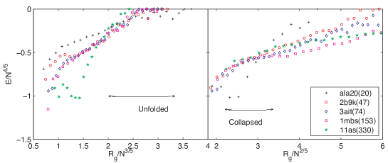
Figure 4: Rescaling the data to exhibit universality in the unfolded state (left) and collapsed state (right) of five proteins, listed with residue numbers in parenthesis. The case $\mathrm{Ala}_{20}$ is exceptional, being completely hydrophobic. Replotted from Lei & Huang, (2009)

From physical arguments, we suggest the following analytical form of the elastic energy:

$$E(R_{g},N)=aN^{4/5}+b(N\,R_{g})^{1/2}+c(\rho)N^{2}/R_{g}^{3}.$$ (22)

Here, $a$ and $b$ are parameters, and $c(\rho)$ represents an effective excluded volume, which depends on $N$ and $R_{g}$ only through the scaled radius

$$\rho=\frac{R_{g}}{N^{2/5}}.$$ (23)

We expect $a$ and $b$ to be universal coefficients, but not the effective excluded volume, as it depends on the intricate structure of a collapsed chain.

The various terms have the following physical meaning:

• The first term $aN^{4/5}$merely establishes the zero point of energy as that of a completely extended chain—a convention used in the CSAW simulations.

• The second term $b(N\,R_{g})^{1/2}$ represents the hydrophobic energy, with $b$ depending on the hydrophobicity of the protein chain.

• The term $c(\rho)N^{2}/R_{g}^{3}$ is a combination of excluded-volume energy and that from hydrogen bonding, and the relative importance of these contributions depends on the scaled radius $\rho$.

Using a phenomenological approach, we expand $c(\rho)$ in an inverse power series of its argument:

$$c(\rho)=\sum_{n\geq 0}c_{n}\rho^{-n}.$$ (24)

Terms of higher $n$ become increasingly important as the collapsed chained is being compressed, and $c(\rho)$ can be positive or negative, depending on the signs of various short-distance interactions.

We fit the parameters $a,b,c_{n}(n=0,\cdots,12)$ to simulation data. Figure 5 shows the fit of (22) to the five proteins used. The fit is poor for $\mathrm{Ala}_{20}$ because of the exceptional nature of the protein as remarked previously. In the case of 11as, simulation has not yet reached an equilibrium ensemble. We did not use these two cases in fitting the parameters.

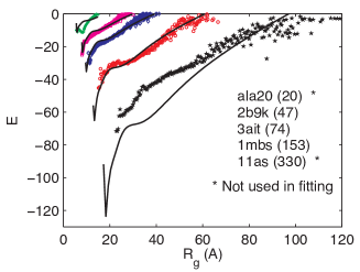
Figure 5: Average potential energy vs. radius of gyration, from computer simulations (points) and the universal elastic energy (22) (solid curves) of five proteins, listed with residue numbers in parenthesis, in the order of the curves from top to bottom. Replotted from Lei & Huang, (2009)

Thus, we have a “universal”elastic energy that should be

• truly universal for large $R_{g}$, when the short-distance interactions are not important, and

• valid only on average at smaller $R_{g},$ when short-distance interactions become important.

7 Stages of protein folding

We identify a stage by the scaling index $\nu$. Such a state is not necessarily stable or metastable, i.e., it does not always correspond to a local minimum of the elastic energy (22). But even an unstable state has kinetic meaning, and we can identify it through physical arguments, by imagining that certain effects are “turned off”.

7.1 Unfolded stage

In the unfolded stage the natural variable is $R_{g}/N^{3/5}$, as revealed by Figure 4 (left panel). In a thought experiment, we can render it stable by imagiing that the hydrophobic effect is turned off. imaging

7.2 The pre-globule

The pre-globule is characterized by $\nu=3/7$. It may or may not be experimentally visible, depending on details of hydrogen bonding. By “turning off”higher-order terms in $c(\rho)$, keeping only the $n=0$ term, we have the elastic energy

$$E_{1}(R_{g},N)=aN^{4/5}+b(NR_{g})^{1/2}+c_{0}N^{2}/R_{g}^{3}.$$ (25)

This has a local minimum with scaling law $R_{g}\sim N^{3/7}$ (Figure 6), which defines the ideal pre-globule theoretically.

Figure 6(b) shows the radius of the ideal pre-globule, which is expected to scale according to

$$R_{g}\approx 4.12N^{3/7}\quad(\mbox{theoretical\ pre-globule}).$$ (26)

This theoretical prediction is larger than observed data, because the hydrogen-bonding attractions have been ignored. By extending the powers in $c(\rho)$ to $n=8$, we find that the local minimum satisfies the scaling law

$$R_{g}\approx 3.61N^{0.41}\quad(\mbox{observed\ pre-globule}),$$ (27)

in good agreement with the pre-globule observed in some proteins (Figure 6) (Uversky,, 2002).

The higher powers in $c\left(\rho\right)$ destabilize the pre-globule, due to the fact that the attractive contributions from hydrogen bonding may make $c(\rho)$ change sign.

“On average”, therefore, the pre-globule is not even metastable, and the collapsed protein chain continues to shrink until it reaches the most compact state, with scaling law $R_{g}\sim N^{2/5}$.

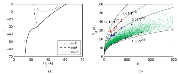
Figure 6: (a). Elastic energy of 1mbs from the potential function (22) with the powers in $c(\rho)$ truncated at $n=0$ (dotted line), $n=8$ (dashed line), and $n=12$ (solid curve), respectively. (b). Radius of gyration for different stages. Theoretical pre-globule: $R_{g}=4.12N^{3/7}$; observed pre-globule: $R_{g}=3.61N^{0.41}$; molten globule: $R_{g}=3.01N^{2/5}$; the most compact state: $R_{g}=1.66N^{2/5}$. Experimental data are also shown, the proteins in pre-globule (triangles) and molten globule (squares) from Tcherkasskaya & Uversky, (2001), the most compact proteins from Arteca, (1995) (circles), and the native proteins from PDB (dots) (Hong & Lei,, 2009).

7.3 The molten globule

In the energy function (22) as plotted in Figure 6(a) (solid line), there is a flat shoulder, which is almost metastable. Between this shoulder and the lowest minimum, corresponding to the most compact state, there is a region that can be identified as the molten globule. We identify this region with a single stage because the scaling exponent is 2/5 throughout. It is bounded by the curves plotted in Figure 6(b):

$$\begin{array}[]{ll}R_{g}\approx 3.01N^{2/5}&(\mathrm{beginning\ of\ molten\ globule}),\\ R_{g}\approx 1.66N^{2/5}&(\mathrm{most\ compact\ state}).\end{array}$$ (28)

As shown in Figure 6(b), data from the PDB show that the $R_{g}$ of all native proteins are distributed between these two curves.

7.4 The native state

The most compact state is the closest we can get to the native state in CSAW, since the detailed structures of the side chains have not been included. As Figure 6(b) shows, the native state in real proteins shares the same scaling index 2/5 with the molten globule. While the time it takes for a random coil to collapse into the molten globule is less than or of the order of microseconds, the development of the molten globule to the native state requires seconds or longer. This suggests that after the molten globule, the “snapping on”of side chains is governed by new mechanisms.

7.5 Mechanisms of different stages

In summary, as shown in Figure 2,

• The unfolded state is characterized by an absence of both hydrophobic forces and hydrogen bonding. The dominant interaction is the excluded-volume effect, which makes the unfolded protein chain a SAW.

• Under hydrophobic forces, the protein chain rapidly collapses into the pre-globule, which is maintained by a balance between the hydrophobic pressure and excluded-volume effect. The density is not high enough for significant hydrogen bonding to occur, and the chain can slide against itself. The lifetime of this state depends on the importance of hydrogen bonding.

• Upon further compression, hydrogen bonding occurs, and the structure acquires rigidity. The protein is now essentially as compact as the native state.

• The side chains “snap on”to native positions, and this process takes a macroscopically long time.

8 Phase transition in myoglobin

The transition from pre-globule to molten globule shows up as a sudden increase in the rate of hydrogen bonding, in a process akin to a phase transition. We illustrate this in the case of myoglobin, as shown in Figure 7 with the number of hydrogen bonds as a function of time.

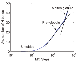
Figure 7: Growth of hydrogen bonds in the simulation of myoglobin. The onset of the transition from pre-globule to molten globule is marked by a sudden jump in the growth rate. Replotted from Lei & Huang, (2009)

9 A theoretical limit on protein size

To describe the effective excluded-volume effect through a single variable depending only on the residue number $N$, we define the “excluded volume”$\bar{c}$ as the average of $c(\rho)$ over all physically possible values of $\rho$:

$$\bar{c}=\dfrac{1}{\rho_{\max}-\rho_{\min}}\int_{\rho_{\min}}^{\rho_{\max}}c(\rho)d\rho,$$ (29)

where $\rho_{\min}$ and $\rho_{\max}$ are respectively the minimum and maximum values of the scaled radius $\rho=R_{g}/N^{2/5}$ in the ensemble.

We have $\rho_{\min}=1.66$ according to the radius of the most compact state given by (28). From Figure 6(b), when there is no hydrogen bonding, the chain collapses to a state with scaling law $R_{g}\approx 4.12N^{3/7}$. This can serve as the maximal radius in the post-collapsed ensemble, and thus

$$\rho_{\max}\approx 4.12N^{1/35}.$$ (30)

Figure 8 shows $\bar{c}$ is a function of $\rho_{\max}$.

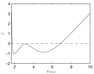
Figure 8: The excluded volume $\bar{c}$ as a function of $\rho_{\max}$.

From Figure 8, we see that $\bar{c}$ changes from negative to positive at $\rho_{\max}\approx 6.85$. When $4.12<\rho_{\max}<6.85$, the excluded volume is negative, and therefore attractive interactions are dominant, which drive the chain to a compact state. When $\rho_{\max}>6.85$, however, the excluded volume is positive, and repulsive interactions are dominant. In this case, the chain cannot fold to a more compact state, because not enough hydrogen bonds can be formed after the hydrophobic collapse.

The value $\rho_{\max}=6.85$ and (30) yield a critical chain length

$$N_{\mathrm{crit}}=5.34\times 10^{7}.$$ (31)

Thus, a super protein ($N>N_{\mathrm{crit}}$) do not have a stable folded state.

We emphasize here that the above conclusion is valid only for a natural protein, i.e., the fraction of hydrophobic residues is around 40% (Hong & Lei,, 2009). It may not be the case for a fully hydrophobic chain.

10 Discussion and outlook

In this chapter, we discuss protein folding from the perspective of statistical physics. We treat the protein as a physical chain immersed in water, and tends towards thermodynamic equilibrium. The process is stochastic, and can be modeled with the master or the Langevin equation. We introduce the CSAW model (conditioned self-avoiding walk), which simulates the Langevin equation for the protein chain. With this model, we are able to study various aspects of protein folding.

In treating protein folding as a physical process, the CSAW model differs from MD in two important aspects, namely

• irrelevant degrees of freedom are ignored; and

• the environment is treated as a stochastic medium.

These, together with simplifying treatment of interactions, enable the model to produce qualitatively correct results with minimal demands on computer time.

An important simplification is the separation of the hydrophobic effect and hydrogen bonding, as expressed by the separate terms in the potential energy. Since both effects arise physically from hydrogen bonding, it is not obvious that we can make such a separation. The implicit assumption is that hydrogen bonding with water involves only the side chains, while internal hydrogen bonding involves only the backbone. This property is supported by statistical data, but should be a result rather an assumption of the model. We should try to remedy this in an improved version of the model.

The CSAW model successfully folds polyalanine ($\mathrm{Ala}_{20}$), a protein fragment of 20 identical amino acids alanine, from random coil to its native state, which is a single alpha helix (Lei & Huang,, 2008). We also use the CSAW model to study the elastic energy of proteins. The elastic energy gives rise to scaling relations of the form $R_{g}\sim N^{\nu}$ in different stages of folding, with $\nu=3/5,3/7,2/5$ for the unfolded stage, the pre-globule, and the molten globule, respectively. The theoretical predictions agree well with experimental data (Figure 6). These stages, together with mechanisms responsible for their formation, are summarized in Figure 2.

These examples show that, despite its simplicity, CSAW incorporates important physical principles governing protein folding.

We can refine CSAW by adding refinements, including the following:

• All-atom side chains with fractional hydrophobicity (Sun,, 2007).

• Electrostatic interactions.

• Replacement of hard-sphere repulsions by Lennard-Jones potentials.

We hope to make progress on the protein folding problem with this theoretical laboratory.

References

- Akiyama et al. , (2003) Akiyama, S, Takahashi, S, Kimura, T, Ishimori, K, Morishima, I, Nishikawa, Y, & Fujisawa, T. 2003. Conformational landscape of cytochrome c folding studied by microsecond-resovled small-angle x-ray scattering. Proc. natl. acad. sci. usa, 99, 1329–1334.
- Alexander et al. , (2005) Alexander, PA, Rozak, DA, Orban, J, & Bryan, PN. 2005. Directed evolution of highly homologous proteins with different folds by phage display: Implications for the protein folding code. Biochemistry, 44, 14045–14054.
- Anfinsen, (1973) Anfinsen, CB. 1973. Principles that govern the folding of protein chains. Science, 181, 223–230.
- Arteca, (1994) Arteca, G. 1994. Scaling behavior of some molecular shape descriptors of polymer chains and protein backbones. Phys. rev. e, 49, 2417–2428.
- Arteca, (1995) Arteca, G. 1995. Scaling regimes of molecular size and self-entanglements in very compact proteins. Phys. rev. e, 51, 2600–2610.
- Arteca, (1996) Arteca, G. 1996. Different molecular size scaling regimes for inner and outer regions of proteins. Phys. rev. e, 54, 3044–3047.
- Baker, (1998) Baker, D. 1998. Metastable states and folding free energy barriers. Nat. struct. biol., 5, 1021–1024.
- Baker & Agard, (1994) Baker, D, & Agard, DA. 1994. Kinetics versus thermodynamics in protein folding. Biochemistry, 33, 7505–7509.
- Berne & Pecora, (1976) Berne, BJ, & Pecora, R. 1976. Dynamic light scattering. New York: Wiley.
- Branden & Tooze, (1998) Branden, C, & Tooze, J. 1998. Introduction to protein structure. New York: Carland Publishing.
- Cecconi et al. , (2005) Cecconi, C, Shank, EA, Bustamante, C, & Marqusee, S. 2005. Direct observation of the three-state folding of a single protein molecule. Science, 309, 2057–2060.
- Chu, (1974) Chu, B. 1974. Light scattering. New York: Academic Press.
- Daggett & Fersht, (2003) Daggett, V, & Fersht, AR. 2003. Is there a unifying mechanism for protein folding? Trends biochem sci, 28, 18–25.
- Day & Daggett, (2003) Day, R, & Daggett, V. 2003. All-atom simulations of protein folding and unfolding. Adv. protein chem., 66, 373–803.
- Dill, (1990) Dill, KA. 1990. Dominant forces in protein folding. Biochemistry, 29, 7133–7155.
- Dill et al. , (2008) Dill, KA, Ozkan, SB, Shell, MS, & Weikl, TR. 2008. The protein folding problem. Annu. rev. biophys., 37, 289–316.
- Doi & Edwards, (1986) Doi, M, & Edwards, SF. 1986. The theory of polymer dynamics. New York: Oxford University Press.
- Duan & Kollman, (1998) Duan, Y, & Kollman, PA. 1998. Pathways to a protein folding intermediate observed in a 1-microsecond simulation in aqueous solution. Science, 282, 740–744.
- Fernandez & Li, (2004) Fernandez, JM, & Li, H. 2004. Force-clamp spectroscopy monitors the folding trajectory of a single protein. Science, 303, 1674–1678.
- Flory, (1953) Flory, P. 1953. Principles of polymer chemistry. New York: Cornell University Press.
- Garrett & Crisham, (1999) Garrett, RH, & Crisham, CM. 1999. Biochemistry. 2nd edn. Thomson.
- He et al. , (2005) He, YN, Yeh, DC, Alexander, PA, Bryan, PN, & Orban, J. 2005. Solution nmr structures of igg binding domains with artificially evolved high levels of sequence identity but different folds. Biochemistry, 44, 14055–14061.
- Hong & Lei, (2009) Hong, L, & Lei, J. 2009. Scaling law for the radius of gyration of proteins and its dependence on hydrophobicity. J. polymer sci. b: Polymer phys., 47, 207–214.
- Huang, (2005) Huang, K. 2005. Lectures on statistical physics and protein folding. Singapore: World Scientific Publishing.
- Huang, (2007) Huang, K. 2007. Conditioned self-avoiding walk (csaw): Stochastic approach to protein folding. Biophys. rev. lett., 2, 139–154.
- Huang, (2009) Huang, K. 2009. Introduction to statistical physics. 2nd edn. London: Taylor & Francis.
- Jang et al. , (2003) Jang, S, Kim, E, Shin, S, & Pak, Y. 2003. Ab initio folding of helix bundle proteins using molecular dynamics simulations. J. am. chem. soc., 125, 14841–14846.
- Kaźmierkiewicz et al. , (2002) Kaźmierkiewicz, R, Liwo, A, & Scheraga, HA. 2002. Energy-based reconstruction of a protein backbone from its -carbon trace by a monte-carlo method. J. comput. chem., 23, 715–723.
- Kaźmierkiewicz et al. , (2003) Kaźmierkiewicz, R, Liwo, A, & Scheraga, HA. 2003. Addition of side chains to a known backbone with defined side-chain centroids. Biophys. chem., 100, 261–280.
- Kennedy, (2002) Kennedy, T. 2002. A faster implementation of the pivot algorithm for self-avoiding walks. J. stat. phys., 106, 407–429.
- Kim & Baldwin, (1990) Kim, PS, & Baldwin, RL. 1990. Intermediates in the folding reactions of small proteins. Annu. rev. biochem., 59, 631–660.
- Kimura et al. , (2005) Kimura, T, Uzawa, T, Ishimori, K, Morishima, I, Takahashi, S, Konno, T, Akiyama, S, & Fujisawa, T. 2005. Specific collapse followed by slow hydrogen-bond formation of -sheet in the folding of signle-chain monellin. Proc. natl. acad. sci. usa, 102, 2748–2753.
- Lau & Dill, (1990) Lau, KF, & Dill, KA. 1990. Theory for protein mutability and biogenesis. Proc. natl. acad. sci. usa, 87, 638–642.
- Lazaridis & Karplus, (2003) Lazaridis, T, & Karplus, M. 2003. Thermodynamics of protein folding: a microscopic view. Biophysical chemistry, 100, 367–395.
- Lei & Huang, (2008) Lei, J, & Huang, K. 2008. Dynamics of alpha helix formation in the csaw model. Eur. phys. j. e, 27, 197–204.
- Lei & Huang, (2009) Lei, J, & Huang, K. 2009. Elastic energy of proteins and stages of protein folding. Europhys. lett., 88, 68004.
- Leong et al. , (2009) Leong, HW, Chew, LY, & Huang, K. 2009. Hamiltonian dynamics of the protein chain and alpha-beta transition. Submitted.
- Levitt, (1976) Levitt, M. 1976. A simplified representation of protein conformations for rapid simulation of protein folding. J. mol. biol., 104, 59–107.
- Li et al. , (1995) Li, B, Madras, N, & Sokal, AD. 1995. Critical exponents, hyperscaling, and universal amplitude ratios for two- and three-dimensional self-avoiding walks. J. stat. phys., 80, 661–754.
- Liu & Deber, (1998) Liu, LP, & Deber, CM. 1998. Uncoupling hydrophobicity and helicity in transmembrane segments: -helical propensities of the amino acids in non-polar environments. J. biol. chem., 273, 23645–23648.
- McCammon et al. , (1977) McCammon, JA, Gelin, BR, & Karplus, M. 1977. Dynamics of folded proteins. Nature, 267, 585–590.
- Michalet et al. , (2006) Michalet, X, Weiss, S, & Jäger, M. 2006. Single-molecule fluorescence studies of protein folding and conformational dynamics. Chem. rev., 106, 1785–1813.
- Moult et al. , (1995) Moult, J, Pedersen, JT, Judson, R, & Fidelis, K. 1995. A large-scale experiment to assess protein structure prediction methods. Proteins: structure, function, and genetics, 23, ii–iv.
- Nielsen et al. , (2004) Nielsen, SO, Lopez, CF, Srinivas, G, & Klein, ML. 2004. Coarse grain models and the computer simulation of soft materials. J. phys.: Condens. matter, 16, R481–512.
- Pauling et al. , (1951) Pauling, L, Corey, RB, & Branson, HR. 1951. The structure of proteins: two hydrogen-bonded helical configurations of the polypeptide chain. Proc. natl. acad. sci. usa, 37(205-211).
- Pearlman et al. , (1995) Pearlman, DA, Case, DA, Caldwell, JW, Ross, SW, Cheatham, TE III, et al. . 1995. Amber, a package of computer programs for applying molecular mechanics, normal-mode analysis, molecular-dynamics and free-energy calculations to simulate the structural and energetic properties of molecules. Comput. phys. commun., 91, 1–41.
- Scheraga et al. , (2007) Scheraga, HA, Khalili, M, & Liwo, A. 2007. Protein-folding dynamics: overview of molecular simulation techniques. Annu. rev. phys. chem., 58, 57–83.
- Shakhnovich, (2006) Shakhnovich, E. 2006. Protein folding thermodynamics and dynamics: where physics, chemistry, and biology meet. Chem. rev., 106, 1559–1588.
- Shental-Bechor et al. , (2005) Shental-Bechor, D, Kirca, S, Ben-Tal, N, & Haliloglu, T. 2005. Monte carlo studies of folding, dynamics, and stability in -helices. Biophys. j, 88, 2391–2402.
- Smith & Hall, (2001) Smith, AV, & Hall, CK. 2001. -helix formation: disctontinuous molecular dynamics on an intermediate-resolution protein model. Proteins: structure, function, and genetics, 44, 344–360.
- Sun, (2007) Sun, W. 2007. Protein folding simulation by all-atom csaw method. Pages 45–52 of: Bioinformatics and biomedicine workshops, bibmw 2007. IEEE International Conference.
- Tcherkasskaya & Uversky, (2001) Tcherkasskaya, O, & Uversky, VN. 2001. Denatured collapsed states in protein folding: Example of apomyoglobin. Proteins: structure, function, and genetics, 44, 244–254.
- Uversky, (2002) Uversky, V. 2002. Natively unfolded proteins: A point where biology waits for physics. Protein sci., 11, 739–756.
- Uversky & Ptitsyn, (1996) Uversky, V, & Ptitsyn, O. 1996. Further evidence on the equilibrium ”pre-molten globule state”: four-state guanidinium chloride-induced unfolding of carbonic anhydrase b at low temperature. J. mol. biol., 255, 215–228.
- Uzawa et al. , (2004) Uzawa, T, Akiyama, S, Kimura, T, Takahashi, S, Ishimori, K, Morishima, I, & Fujisawa, T. 2004. Collapse and search dynamics of apomyoglobin folding revealed by submilisecond observations of -helical content and compactness. Proc. natl. acad. sci. usa, 101, 1171–1176.
- van Kampen, (1992) van Kampen, NG. 1992. Stochastic processes in physics and chemistry. 2nd edn. Amsterdam: North-Holland.
- Zhang, (2008) Zhang, Y. 2008. Progress and challenges in protein structure prediction. Curr. opin. struct. biol., 18, 342–348.
- Zhang & Skolnick, (2005) Zhang, Y, & Skolnick, J. 2005. The protein structure prediction problem could be solved using the current pdb library. Proc natl acad sci usa, 102, 1029–1034.