Coarse-Grained Models of Biological Membranes within
the Single Chain Mean Field Theory

Abstract

The Single Chain Mean Field theory is used to simulate the equilibrium structure of phospholipid membranes at the molecular level. Three levels of coarse-graining of DMPC phospholipid surfactants are present: the detailed 44-beads double tails model, the 10-beads double tails model and the minimal 3-beads model. We show that all three models are able to reproduce the essential equilibrium properties of the phospholipid bilayer, while the simplest 3-beads model is the fastest model which can describe adequately the thickness of the layer, the area per lipid and the rigidity of the membrane. The accuracy of the method in description of equilibrium structures of membranes compete with Monte Carlo simulations while the speed of computation and the mean field nature of the approach allows for straightforward applications to systems with great complexity.

I Introduction

Phospholipid membranes and self-assembled bilayers of block copolymers have many common features originating from the amphiphilic nature of the molecules. Phospholipids comprise of hydrophilic head group and two hydrophobic acyl chains and the driving force of self-assembly in membranes, as in case of block copolymers, is the hydrophobic effect Lipowsky and Sackmann (1995). Thus, theoretical methods developed for the self-assembly of block copolymers can be applied for the description of phospholipid membranes Muller et al. (2006).

Theoretical description and computer simulation of phospholipid bilayers and biological membranes is a challenging task for many decades Muller et al. (2006); Venturolia et al. (2006). Although phospholipids are relatively short chains in comparison to polymers and block copolymers, the configurational space of conformations and the number of interactions are extremely large. In addition, the simulation of phospholipid bilayers and membranes is a problem involving many interacting molecules, thus full description of collective behavior would require simultaneous simulation of a large number of molecules. That is why, full atomistic molecular dynamics models Tieleman et al. (1997); Damodaran et al. (1992); Damodaran and Merz (1994); Smondyrev and Berkowitz (1999); Robinson et al. (1994); Heller et al. (1993); Tuckerman et al. (1992); Lyubartsev (2005); Hyvonen et al. (1997), describing membranes with chemical accuracy, are limited to short times and short lengths. Usually, atomistic models on times exceeding microseconds and lengths larger than nanometers are not practical Muller et al. (2006), especially when the equilibrium structures of large systems are considered.

One of the strategy to overcome this problem is to group atoms into effective particles that interact via effective potentials within so-called coarse-grained models Kotelyanskii and Theodorou (2004). Coarse-graining can reduce considerably the degrees of freedom and the configurational space such that larger systems and longer times can be reached. Monte-Carlo (MC) simulations of phospholipid membranes with coarse-grained models of phospholipids Goetz and Lipowsky (1998); Shelley et al. (2001, 2001); Muller et al. (2003); Marrink et al. (2004); Cooke et al. (2005) are proved to capture the essential properties of self-assembly of phospholipids into membranes, their molecular structure and collective phenomena.

However, if the objective of the research is the equilibrium properties and the molecular details of the self-assembled structures, the equilibration time may largely exceed microseconds and thus, may not be reached with MD simulations in a reasonable time. Alternative strategy is to reach directly the minimum of the free energy using methods based on mean field theories, thus, avoiding computationally expensive equilibration process used in MC and MD simulations.

The method of the Single Chain Mean Field (SCMF) theory Ben-Shaul et al. (1985, 1986); Mackie et al. (1997); Al-Anber et al. (2005, 2003); Shvartzman-Cohen et al. (2009) is particularly suitable for such purposes: it combines analytical theory of the mean field type with the conformational variability accessible in MC simulations. Thus, the accuracy of the method in describing the molecular details of equilibrium structures can compete with MC simulations while the speed of obtaining the results depends only on the speed of the numerical solution of equations, thus it can be much faster than MC simulations.

The advantage of this method is the speed in localization of the free energy minimum and the equilibrium properties as well as the precision in the measurement of the equilibrium free energy which is not straightforwardly accessible with MD and MC simulations. The disadvantage is the mean-field nature of the solution that does not include fluctuations and inter-particle correlations. Nevertheless, the shortcomings of the approach can be compensated by the combination of the SCMF theory with MD simulations which can complement the method. Fast mean field method provides for equilibrium structure with molecular details which, in turn, can be used as input initial configuration for MD simulations and provide the lacking dynamic information and fluctuations.

The SCMF theory, originally developed for the micellization problem of low-molecular surfactants Ben-Shaul et al. (1985, 1986), describes a single molecule in the molecular fields. The multichain problem is reduced to a single chain in the external self-consistent field problem. The position, orientation and configuration of the molecule depend on the surrounding fields while the fields depend on the configurations of the molecules, and finally the equilibrium fields are found self-consistently by numerical solution of a system of nonlinear equations. This method gives a detailed microscopic information on the configurations and averaged positions of the molecules, the optimal shape and structure of self-assembled structures, the distribution of molecules in the aggregates, the critical micellar concentrations as well as the optimal aggregation number and the size distributions of the micelles and the aggregates Al-Anber et al. (2005, 2003). This method is quite universal: it can be applied to solutions of linear or branched polymers, solutions of low-molecular weight surfactants and various additives, mixtures of various components and structural and shape transitions. However, the limiting factor restraining the use of the SCMF theory is the computational realization of a stable code that can efficiently solve self-consistent equations. There are no standard packages with universal implementation of the SCMF theory, which could make the use of the method accessible for a large number of people like Mesodyn package Altevogt et al. (1999); Fraaije et al. (1997) for mesoscopic modeling of phase separation dynamics or an integrated simulation system for soft materials (OCTA) for multiscale modeling Doi (2003); Soldera et al. (2009); Mae et al. (2008). Most of the previous works on SCMF theory Ben-Shaul et al. (1985, 1986); Mackie et al. (1997); Al-Anber et al. (2005, 2003) use iterative methods or external mathematical libraries, which are not optimized for a given problem and thus, computationally unstable and highly demanding in computer resources, especially in RAM memory. Thus, problems involving long molecules, large systems and geometries more than 1D confront with the limit of available computer resources and thus, making the solution of the problem without special technical skills to be a quite difficult task. A modification of the method, Single Chain in Mean Field calculations Muller and Smith (2005); Daoulas et al. (2006); Daoulas and Muller (2006), avoids the necessity to solve self-consistent equations. The direct solution of the self-consistent equations is replaced by MC equilibration of the chains in the quasi-instantaneous fields maintained at the most recent values and updated after a predetermined number of MC moves. In practice, the MC equilibration would slow down the calculation with respect to direct solution of the equations, but it is still much faster than the direct MC method.

It is noteworthy that SCMF method is similar in spirit to one of the first mean field model of the phospholipid membranes by Marcelja Marcelja (1973, 1974) constructed for modeling of the fluid – gel phase transition and based on phenomenological potential of the Maier-Saupe type between the segments of the tails. The boundary between the solvent and the membrane is modeled as a planar surface with the phospholipid tails attached with a fixed grafting density. Each tail interacts with the neighbors via mean field which is found self-consistently.

In this work we report a computational tool providing relatively fast and stable solution of the equations of the SCMF theory in different geometries and different molecule structures. The SCMF theory is applied to model phospholipid membranes. We show that three different coarse-grained models of phospholipids can adequately describe the equilibrium properties and the molecular structure of phospholipid membranes.

The paper is organized as follows. Theoretical principles of the SCMF theory and main equations of the method are introduced in the section II in the most general way. This theory is then applied to the simulation of phospholipid bilayers and three coarse-grained models of phospholipid molecule are introduced in section III. These models and the resulting equilibrium phospholipid bilayers are compared with experimental data and between each other in section IV. Last section V summarizes the obtained results while the computational details which are necessary for the implementation of the method are described in the Appendix A.

II Theory

The SCMF theory is an example of the Self-Consistent Field (SCF) method where a single chain is described at the molecular level while the interactions between different chains are described through a mean molecular field which is found self-consistently.

The conformations of a single chain are generated with the Rosenbluth algorithm Rosenbluth and Rosenbluth (1955) or MC simulations Kotelyanskii and Theodorou (2004); Frenkel and Smit (2002) and the intra-molecular interactions are calculated exactly using the model potential for interactions between the segments of the chain (see Appendix A.1 for details). The probabilities of individual chain conformations depend on the mean molecular fields, while the values of the fields are calculated as the average properties of individual conformations. The resulting equations for the mean fields and the probabilities of the conformations are solved self-consistently with the original method described in the Appendix A.3. The solution of these equations gives the equilibrium structures and the concentrations profiles of all components in the system as well as the most probable conformations of individual molecules. The power of this method is the speed in obtaining solutions (faster than MC and much faster than MD simulations) and the precise calculation of the energies.

This method is quite universal and can be applied for the mixture of an arbitrary number of molecules of different types interacting with each other through the mean fields. The free energy of a system containing $N_{1},N_{2},...,N_{M}$ molecules of types $1,2,...,M$ can be written as a sum of three terms, the entropy, intra- and inter-molecular terms, all written in terms of $kT$,

$$F=-\left\langle S\right\rangle+\left\langle H^{intra}\right\rangle+\left\langle H^{inter}\right\rangle$$ (1)

where the angular brackets denote the average over the probability distribution function (pdf) $\rho$ of the system, $\left\langle\ldots\right\rangle=\int\ldots\rho d\rho$. This function contains all information about the equilibrium state of the whole system. If there are no strong correlations between interacting particles, such as ion pair formation or bonds formation, we can neglect the correlations between the molecules and use the mean field approximation: the pdf $\rho$ of many component system factorizes into the product of single molecules pdfs $\rho_{\alpha}(\Gamma_{\alpha i})$,

$$\rho\approx\prod_{\alpha=1}^{M}\prod_{i=1}^{N_{\alpha}}\rho_{\alpha}(\Gamma_{\alpha i})$$ (2)

where $\Gamma_{\alpha i}$ is the conformation of $i$-th molecule of type $\alpha$. Such factorization into contributions of individual molecules allows us to derive a close set of equations for $\rho_{\alpha}(\Gamma_{\alpha i})$.

The entropy term in the expression (1) is written as

$$\left\langle S\right\rangle=-\left\langle\ln\rho\Lambda\right\rangle,\quad$$ (3)

where the factor $\Lambda$ is the de Broglie length which has a quantum mechanics origin,

$$\Lambda=\prod_{\alpha=1}^{M}\Lambda_{\alpha}^{N_{\alpha}}N_{\alpha}!\approx\prod_{\alpha=1}^{M}\left(\frac{N_{\alpha}\Lambda_{\alpha}}{e}\right)^{N_{\alpha}}$$ (4)

Since the constants $\Lambda_{\alpha}$ do not appear in the final expressions, they can be treated as unknown normalization constants. Thus, after factorizing the pdf $\rho$ (2), the entropy term (3) reads

$$\left\langle S\right\rangle\approx-\sum_{\alpha=1}^{M}N_{\alpha}\left\langle\ln\frac{\rho_{\alpha}N_{\alpha}}{e}\Lambda_{\alpha}\right\rangle$$ (5)

where the brackets on the right hand side denote the average over the single molecule pdf $\rho_{\alpha}$. Similar arguments allow us to write the intra-molecular energy of the system as a sum of contributions of the single molecules of different types

$$\left\langle H^{intra}\right\rangle\approx\sum_{\alpha=1}^{M}N_{\alpha}\left\langle H_{\alpha}^{intra}\right\rangle$$ (6)

Before writing a similar expression for the inter-molecular part, we assume that molecules of each type $\alpha$ comprise of subunits with different chemical structure, and thus different energy parameters. Subunits can represent Kuhn segments in the chain or, in case of coarse-graining description, the groups of atoms or beads in a coarse-grained model. Thus, the interaction energy between a molecule of type $\alpha$ in the conformation state $\Gamma_{\alpha}$ and a molecule of type $\beta$ in the conformation state $\Gamma_{\beta}$, can be written as a sum over the types of beads $a$ as

$$H_{\alpha\beta}^{inter}\left(\Gamma_{\alpha},\Gamma_{\beta}\right)=\sum_{a}\int u_{\alpha}^{a}(\Gamma_{\alpha},\boldsymbol{r})c_{\beta}^{a}(\Gamma_{\beta},\boldsymbol{r})d\boldsymbol{r}$$ (7)

In this expression $c_{\beta}^{a}(\Gamma_{\beta},\boldsymbol{r})$ is the concentration of units of type $a$ at the point $\boldsymbol{r}$ of a molecule of type $\beta$ in the conformation state $\Gamma_{\beta}$. These units interact with the field $u_{\alpha}^{a}(\Gamma_{\alpha},\boldsymbol{r})$ created by the molecules of type $\alpha$. Thus, factorizing the pdf $\rho$ (2) one can write the inter-molecular interaction free energy in the form

$$\left\langle H^{inter}\right\rangle\approx\frac{1}{2}\sum_{\alpha,\beta=1}^{M}N_{\alpha}(N_{\beta}-\delta_{\alpha\beta})\sum_{a}\int\left\langle u_{\alpha}^{a}(\boldsymbol{r})\right\rangle\left\langle c_{\beta}^{a}(\boldsymbol{r})\right\rangle d\boldsymbol{r}$$ (8)

where $\delta_{\alpha\beta}$ is the delta symbol. Thus, the interaction free energy is represented by the interaction of the average concentration of beads with the average fields at each point.

The free energy is usually coupled with the incompressibility condition implying that the sum of the concentrations of all components in a solution is fixed. However, this condition implies the hard core repulsion between all beads in the system, and thus creates computational problems in converging the SCMF equations. To overcome this problem, we introduce the explicit incompressibility condition in every point $\boldsymbol{r}$ in the system,

$$\sum_{\alpha=1}^{M}N_{\alpha}\left\langle\phi_{\alpha}(\boldsymbol{r})\right\rangle=\phi_{0}$$ (9)

where $\left\langle\phi_{\alpha}(\boldsymbol{r})\right\rangle$ is the average volume fraction occupied by a molecule of type $\alpha$ in the point $\boldsymbol{r}$, while $\phi_{0}$ is the total volume fraction occupied by the molecules of all types.

Combining all terms (5), (6), (8) together with the incompressibility condition (9), the free energy of the system can be written as

$$\begin{split}&F[\rho_{1},\rho_{2},...,\rho_{M}]\approx\sum_{\alpha=1}^{M}N_{\alpha}\left\langle\ln\frac{\rho_{\alpha}N_{\alpha}}{e}\Lambda_{\alpha}\right\rangle+\\ &\sum_{\alpha=1}^{M}N_{\alpha}\left\langle H_{\alpha}^{intra}\right\rangle+\\ &\frac{1}{2}\sum_{\alpha,\beta=1}^{M}N_{\alpha}(N_{\beta}-\delta_{\alpha\beta})\sum_{a}\int\left\langle u_{\alpha}^{a}(\boldsymbol{r})\right\rangle\left\langle c_{\beta}^{a}(\boldsymbol{r})\right\rangle d\boldsymbol{r}+\\ &\int\lambda(\boldsymbol{r})\left(\phi_{0}-\sum_{\alpha=1}^{M}N_{\alpha}\left\langle\phi_{\alpha}(\boldsymbol{r})\right\rangle\right)d\boldsymbol{r}\end{split}$$ (10)

where $\lambda(\boldsymbol{r})$ is a Lagrange multiplier and all the averages are taken over the single-molecule pdfs $\rho_{\alpha}$. Minimization of this functional with respect to $\rho_{\alpha}$ gives the pdf of a single molecule of type $\alpha$

$$\rho_{\alpha}(\Gamma_{\alpha})=\frac{1}{Z_{\alpha}}\exp\left(-H_{\alpha}^{intra}(\Gamma_{\alpha})-\sum_{\beta=1}^{M}(N_{\beta}-\delta_{\alpha\beta})\times\right.$$

$$\left.\sum_{a}\int u_{\alpha}^{a}(\Gamma_{\alpha},\boldsymbol{r})\left\langle c_{\beta}^{a}(\boldsymbol{r})\right\rangle d\boldsymbol{r}+\int\lambda(\boldsymbol{r})\phi_{\alpha}(\Gamma_{\alpha},\boldsymbol{r})d\boldsymbol{r}\right)$$ (11)

where $Z_{\alpha}$ is a normalization constant which is found from the normalization condition $\int\rho_{\alpha}(\Gamma_{\alpha})d\Gamma_{\alpha}=1$. This constant has a meaning of a partition function of the system at equilibrium and $-\ln Z_{a}$ is the total free energy of the system at equilibrium.

Once the average concentrations $\left\langle c_{\beta}^{a}(\boldsymbol{r})\right\rangle$ and the volume fractions $\left\langle\phi_{\beta}(\boldsymbol{r})\right\rangle$ are known, this expression allows to calculate the probabilities of each conformation $\rho_{\alpha}(\Gamma_{\alpha})$ for all molecules in the system. In turn, if the probabilities $\rho_{\alpha}(\Gamma_{\alpha})$ are known, the average concentrations and volume fractions, being the the molecular fields in this problem are found from the self-consistency conditions,

$$\left\langle c_{\alpha}^{a}(\boldsymbol{r})\right\rangle = \int c_{\alpha}^{a}(\Gamma_{\alpha},\boldsymbol{r})\rho_{\alpha}(\Gamma_{\alpha})d\Gamma_{\alpha}$$ (12)

$$\left\langle\phi_{\alpha}(\boldsymbol{r})\right\rangle = \int\phi_{\alpha}(\Gamma_{\alpha},\boldsymbol{r})\rho_{\alpha}(\Gamma_{\alpha})d\Gamma_{\alpha},$$

representing the averages over the probabilities of conformations.

The probability of each conformation can be written as $\rho_{\alpha}(\Gamma_{\alpha})=\frac{1}{Z_{\alpha}}\exp[-H_{eff}(\Gamma_{\alpha})]$, where $H_{eff}(\Gamma_{\alpha})$ is the effective Hamiltonian given by (11), which describes the system at equilibrium. The last term in the effective Hamiltonian corresponds to the steric repulsion of beads of all types. If one of the components is a one bead solvent, the only degree of freedom of the solvent molecules is the position in space, $\boldsymbol{r}$. Hence, the volume fraction of the solvent, can be found from the incompressibility condition (9)

$$\phi_{s}(\boldsymbol{r})=\phi_{0}-\sum_{\alpha=1,\alpha\neq s}^{M}N_{\alpha}\left\langle\phi_{\alpha}(\boldsymbol{r})\right\rangle$$ (13)

In addition, the Lagrange multiplier $\lambda(\boldsymbol{r})$ can be expressed through the concentration of the solvent. The pdf of the solvent $\rho_{s}(\boldsymbol{r})$, the concentration $c_{s}(\boldsymbol{r})$ and the volume fraction occupied by the solvent $\phi_{s}(\boldsymbol{r})$ are related via the following expressions

$$\rho_{s}(\boldsymbol{r})=\frac{c_{s}(\boldsymbol{r})}{N_{s}}=\frac{\phi_{s}(\boldsymbol{r})}{v_{s}N_{s}}\quad$$ (14)

where $N_{s}$ is the number and $v_{s}$ is the volume of the solvent molecule, while the molecular field

$$\phi_{s}(\boldsymbol{r},\boldsymbol{r}^{\prime})\approx v_{s}\delta(\boldsymbol{r}-\boldsymbol{r}^{\prime})$$ (15)

where $\delta(\boldsymbol{r}-\boldsymbol{r}^{\prime})$ is the Dirac delta-function. Substitution of (14) and (15) into (11) gives the approximate expression for the Lagrange multiplier $\lambda(\boldsymbol{r})$

$$v_{s}\lambda(\boldsymbol{r})\approx\ln\phi_{s}(\boldsymbol{r})+\sum_{\beta=1}^{M}(N_{\beta}-\delta_{s\beta})\sum_{a}\int u_{s}^{a}(\boldsymbol{r},\boldsymbol{r}^{\prime})\left\langle c_{\beta}^{a}(\boldsymbol{r}^{\prime})\right\rangle d\boldsymbol{r}^{\prime}$$ (16)

where we have assumed that $H_{s}^{intra}(\boldsymbol{r})=0$ and omitted few constants, which will cancel out by the normalization of $\rho_{\alpha}$.

It is noteworthy, that in our equations the fields $\left\langle\phi_{\alpha}(\boldsymbol{r})\right\rangle$ and $\left\langle c_{\alpha}^{a}(\boldsymbol{r})\right\rangle$ formally are not related although they both correspond to the concentration of monomers. They are indeed related through the volume of the monomers only if the molecules are composed of non-overlapping beads, when the distance between the centers is larger than the the diameter. However, if we want to conserve the possibility of describing the overlapping beads, the coefficient of proportionality between $\left\langle\phi_{\alpha}(\boldsymbol{r})\right\rangle$ and $\left\langle c_{\alpha}^{a}(\boldsymbol{r})\right\rangle$ is not known a priori and we keep them as independent variables.

The equations (11),(12),(13) and (16) form a closed set of non-linear equations of the SCMF theory. The solution of these equations gives the equilibrium structures, the self-consistent molecular fields such as the concentration profiles of the beads of each type and the distribution of the solvent, and the probabilities of each conformation of the molecules in the fields and the accurate measure of equilibrium free energies. The implementation of the computational method as well as the technical details related to the solution of the equations are present in Appendix A.

III Application to phospholipid membranes

The method of the SCMF theory described so far is applied to model the equilibrium structures and properties of phospholipid membranes. The SCMF theory can provide the detailed information on the microscopic structure of the phospholipid layer such as concentration profiles of all groups of atoms of the phospholipid molecule, the thickness of the membrane, the average area per phospholipid head group and the mechanical properties such as compressibility of the membrane and the surface tension. All these parameters can be measured in the experiment Kucerka et al. (2005); Nagle and Tristram-Nagle (2000); Mathai et al. (2008) and thus, allowing the direct comparison with experimental data.

We have developed the C++ code which runs in parallel using OpenMP shared memory platform on the 32-core AMD machines (see Appendix A.3). To simulate a flat phospholipid layer we use one dimensional geometry and discretize the space into parallel cells with the same value of the average fields. The periodic boundary condition is applied together with the assumption of the symmetry of the layer with respect to the central plane.

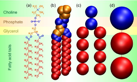
Figure 1: (a) Chemical structure of the DMPC phospholipid molecule. 44-beads (b), 10-beads (c) and 3-beads (d) models of phospholipid molecules used in the present calculations. Blue beads correspond to hydrophilic monomers, red beads correspond to hydrocarbon monomers in the tails and orange beads correspond to hydrophobic monomers in the heads. The interaction parameters of red and orange beads are the same.

Despite the complexity of the structure of the phospholipid membranes, the driving force for the self-assembly of phospholipids into bilayers is the amphiphile nature of phospholipids. That is why, we only consider the units of two types, hydrophilic, H, and hydrophobic, T. The units of both types interacts with each other through the square well potentials. We assume that all units, T and H, and the solvent molecules S, have the same size and the same interaction range, while the interaction energies are different. We consider three types of interactions, interactions between hydrophobic units, T-T, interactions between hydrophobic units and solvent, T-S and hydrophilic units with solvent, H-S. In the following we will show that such assumptions are justified for quantitative study of phospholipid layers and, in principle, cohere with approximations used in successful models of phospholipid membranes (see e.g. Ref. 19). However, if necessary, more types of beads and more complicated potentials can be implemented.

Table 1: Parameters used for the simulation of phospholipid bilayer for three models of DMPC phospholipid molecule.

	44B	10B	3B
Units radius (Å)	$1.90$	$2.50$	$4.05$
Interaction range (Å)	$5.70$	$7.50$	$12.15$
T-T contact energy ($kT$)	$-0.40$	$-1.50$	$-2.10$
T-S contact energy ($kT$)	$0.00$	$0.00$	$0.00$
H-S contact energy ($kT$)	$-0.10$	$-0.20$	$-0.15$
Bond length (Å)	$1.5$	$5.0$	$10.0$
Occupied volume fraction $\phi_{0}$	$0.700$	$0.675$	$0.675$
Sampling (number of configurations)	$3\times 10^{6}$	$10^{6}$	$10^{6}$
Simulation box size (Å)	$120.0\times 120.0\times 62.7$

The chemical structure of the DMPC molecule is depicted in Figure 1a. We present three models of DMPC phospholipid molecule at a different level of coarse-graining.The first, most detailed model, represents the DMPC phospholipid as a two tails molecule of 44 beads (Figure 1b). A carbon group CH2 of the molecule is assigned to one T bead. A phosphate group, PO4, is represented by 5 H overlapping beads, placed at the vertexes and center of a tetrahedron. The choline group NC4H11 is represented in a similar way: one H bead in the center of a tetrahedron is surrounded by 4 T beads placed in the corners. The COO groups are represented by 2 H beads. The angles between most of the bonds are fixed at value $120^{\circ}$. The torsion angles the sequence of groups CH2-CH2-CH2 are allowed to have only three fixed values, $0^{\circ}$, $120^{\circ}$ and $240^{\circ}$, which corresponds to cis- and trans- conformations of the groups. The parameters of the model (Table 1) were adjusted with a series of fast simulations (conformational sampling size $\sim 30-100$ thousands and $40$ layers in the simulation box) while the accurate data were obtained with several millions of conformations and hundred layers in the box.

Two others, more coarse-grained and less detailed, models are depicted in Figures 1c and 1d. One of them represents two tails phospholipid with 10 beads and another is simply 3-beads freely joined together. In contrast to 44-beads model, the conformational space of these models is much more restricted and we need less sampling to produce accurate results. Thus, the simplest 3-beads model is the fastest and demanding less computer resources phospholipid model which can simulate the self-assembly of phospholipids into the bilayers with realistic properties of DMPC phospholipid membranes.

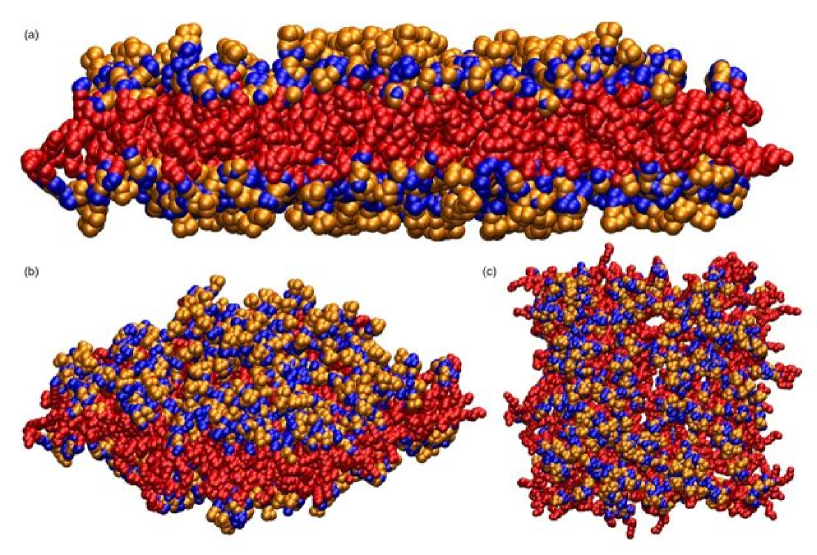
Figure 2: Typical mean field ”snapshots” (set of most-probable conformations of the lipids) of the phospholipid membrane within the 44-beads model.

It is important to note, that we simulate a finite size box with the fixed volume $V$ and the fixed number of phospholipid molecules $N_{l}$ with the free energy $F$ given by the expression (10). However, we can extrapolate our data to much larger system with larger number of phospholipids $N_{l}^{\ast}$ and larger number of solvent molecules. The description of a larger system is possible, if we do not take into account any energy contributions related to the perpendicular undulations and bending of the membrane. In this case the simulation box represent a self-similar part of a larger system. The free energy of the larger system $F^{\ast}$ is in a simple relation with the free energy per lipid $f$

$$F^{\ast}\approx{const}+N_{l}^{\ast}f$$ (17)

which, in turn, is related to the free energy of the simulation box minus the entropy of the solvent

$$fN_{l}=F-V\frac{\phi_{0}}{v_{s}}\ln\frac{\phi_{0}}{v_{s}}$$ (18)

where $\phi_{0}/v_{s}$ is the concentration of the pure solvent.

Thus, the calculation of free energy of the box $F$ with different number of molecules in the simulation box gives the free energy of the membrane per lipid $f$. The minimum of the free energy per lipid $f$ corresponds to the equilibrium density of the membrane, thus the second derivative of this energy with respect to the area per lipid in the minimum gives the compressibility modulus of the layer

$$K=2A_{eq}f^{\prime\prime}(A_{eq})$$ (19)

representing a measure of the rigidity of the membrane.

IV Results and discussion

The numerical implementation of the method in the form of two structurally independent modules: the generation of a single molecule conformations and the solution of equations (see Appendix A), permits us to consider several models of the molecule at the same time. Thus, we can compare our three models of phospholipids and test their performance in reproducing the thermodynamic properties of phospholipid membranes.

The most detailed 44-beads model (Figure 1b) results in equilibrium structures of membranes where the phospholipids are assembled into flat bilayers in fluid phase. Since the output of the method is the probabilities of each molecular conformation in the self-consistent fields, the most probable conformations may be used for the visualization of the resulting structures which correspond to the solutions of the equations. Typical mean field ”snapshots” of the equilibrium bilayer structures obtained with the 44-beads model are present at Figure 2. Although the picture visually resemble instant snapshots of MC simulations, this is not a representation of interacting molecules at a given moment of time, but these are the most probable conformations of a single chain in the fields corresponding to the equilibrium solution. Such ”snapshots” are helpful for visualization purposes in order to distinguish between different molecular structures.

The equations of the SCMF theory may result in several sets of solutions corresponding to various equilibrium and even metastable structures. To this end, the numerical method is implemented in such a way that simultaneously several solutions corresponding to local and global minima of the free energy can be found. The obtained solutions can then be ranged by their free energy or by the concentration profile. Even in the restricted 1D geometry of flat phospholipid bilayers with periodic boundary condition the method finds several self-assembled structures: homogeneous solution of lipids, one single layer, formed either at the center or at the edge of the box and two or even three layers in the box. Each structure has its own free energy which allows to determine the equilibrium properties.

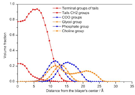
Figure 3: Detailed equilibrium concentration profile of the phospholipid bilayer obtained with the 44-beads model.

The detailed microscopic information concerning the mechanic and thermodynamic properties of the simulated flat bilayers can be compared directly against the experimental data for phospholipid bilayers Kucerka et al. (2005); Nagle and Tristram-Nagle (2000); Mathai et al. (2008). Thermodynamic properties of the membranes obtained from the measurements are the thickness of the membrane (determined as a distance between the midpoints of the outer slopes of the H beads concentration profiles), the full thickness of the bilayer region (determined as a thickness of the region where the total concentration of the lipid molecules is larger than zero), the thickness of the hydrophobic core (measured as a distance between the midpoints of the slopes of the T beads concentration profiles), the distances between different groups of the phospholipid molecule, membrane rigidity measured by the compressibility modulus and the interfacial area per lipid molecule. Thus, the coarse-grained parameters of each model of phospholipid molecule are chosen in such a way that all these microscopic properties correspond to the experimental values of the DMPC phospholipid bilayers. The parameters of these three models are summarized in Table 1.

Table 2: Comparison of the equilibrium properties of phospholipid bilayer obtained with three lipid models with experimental data and full atomistic MD simulations of the DMPC lipid bilayer.

	44B	10B	3B	DMPC
Membrane thickness (Å)	35	36	45	$44.2$a
Full thickness of the bilayer region (Å)	51	44	56	$53$b
Thickness of hydrophobic core (Å)	24	24	28	$26.2$a
Distance between heads (Å)	30	28	36	$36$a
Distance between phosphate groups (Å)	30	-	-	$32$b
Distance between choline groups (1st peak) (Å)	22	-	-	$37$b,d
Distance between choline groups (2nd peak) (Å)	42	-	-	$37$b,d
Distance between glycol groups (Å)	26	-	-	$27$b
Distance between COO groups (Å)	24	-	-	$25$b
Thickness of terminal groups region (Å)	6	-	-	$10$b
Interfacial area per lipid (Å2)	$70\pm 5$	$65\pm 11$	$60\pm 2$	$59.6$a
Compress. constant (dyn/cm)	$135\pm 11$	$560\pm 120$	$269\pm 11$	$257$c

^a Experimental data by Nagle and Tristram-NagleNagle and Tristram-Nagle (2000)

^b Calculated from MD simulations data by Damodaran and Merz Damodaran and Merz (1994)

^c Experimental data by Mathai et al.Mathai et al. (2008)

^d Average distance between choline groups.

The most detailed 44-beads model provides all information about the composition of the membrane as well as the position of different groups of the molecule in the bilayer. The concentration profile of the bilayer at equilibrium is shown in Figure 3. The profiles are normalized to unity by division by the occupied volume fraction $\phi_{0}$. One can see, that the terminal groups of the lipid tails are situated in the center of the layer, which is surrounded by the area filled with other carbon groups of the tails. The groups of hydrophilic units representing the “heads” are in the surface layer. Such position of the groups is in agreement with the experimental data for such system Nagle and Tristram-Nagle (2000). It is noteworthy, that the concentration profile of choline group has two peaks reflecting the position of phospholipid heads in the layer: approximately half of the heads are oriented perpendicular to the layer plane, while the other half is parallel to the layer plane. This is the outcome of the model of the phospholipid molecule and the parametrization of the interactions. This can certainly be improved once the reliable experimental data or results of MD simulations concerning the equilibrium position of the heads in the layer is available.

One of the advantages of the SCMF method is the accurate measurements of the free energies of equilibrium structures. In our model this corresponds to the free energy of formation of flat phospholipid layer. It does not include the entropy of thermal undulations in the perpendicular direction. In particular, undulations may result in the broadening of the phospholipid membrane. However, they become important on the scales much larger than the size of the simulation box and, in principle, can be included as an additional contribution to the free energy of the layer.

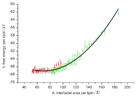
Figure 4: Free energy per lipid $f$ vs. interfacial area per lipid $A$ for the 44-beads lipid model, calculated from solutions with one (red points) and two (green points) bilayers in the simulation box. Parameters of the fitting curve $y=a_{0}+a_{1}x+a_{2}x^{2}$ are $a_{0}=-61.3\pm 0.5$, $a_{1}=-0.164\pm 0.010$, $a_{2}=(1.17\pm 0.04)\times 10^{-3}$.

The rigidity of the membrane can be obtained from the free energy of the bilayer. Changing the number of lipids in the box, we get the free energy per lipid molecule $f$ as a function of the interfacial area per lipid $A$ (Figure 4). Although the error bars are quite large because of the large conformational space with respect to the sampling used for the calculations, the energy points can be quite good approximated with the polynomial of the second order. This curve allows us to calculate the compressibility of the layer with respect to compression and stretching in the lateral direction. The second derivative is related to the compressibility modulus defined in eq. (19). The resulting compressibility modulus, the thickness of the membrane, positions of various groups and the area per lipid are shown in Table 2. The obtained values agree quite well with the experimental data. However, if better agreement is needed, the parameters of the models can be tuned by the additional series of run of calculations with a large number of conformations in the sampling.

The free energy per lipid $f$ (Figure 4) has a minimum at $A\approx 60$Ų, which corresponds to the experimental value of the interfacial area per lipid in the bilayer in the fluid phase. Howether, the values of $A$ below $50$Ų cannot be obtained with the same set of parameters, because this range corresponds to dense packing in the core of the layer. Further decrease of interfacial area per lipid is accompanied with structural rearrangements of the phospholipid environment and strong correlations between the neighboring molecules. These correlations induce phase transitions in lipid membranes Koynova and Caffrey (1998), the main transition to the gel phase occurs at $A\approx 40$Ų. However, such correlations are well beyond the limit of validity of the mean field theory, where the movements of individual molecules are supposed to be uncorrelated (2).

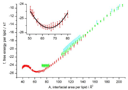
Figure 5: Free energy per lipid $f$ vs. interfacial area per lipid $A$ for the 10-beads lipid model, calculated from solutions with one (red points), two (green points) and three (blue points) bilayers in the simulation box. The inset represents the enlarged region of the minimum. Parameters of the fitting curve $y=a_{0}+a_{1}x+a_{2}x^{2}$ are $a_{0}=-3.0\pm 3.0,$ $a_{1}=-0.68\pm 0.08,$ $a_{2}=(5.2\pm 0.6)\times 10^{-3}$.

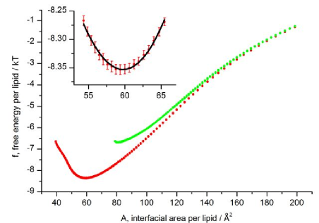
Figure 6: Free energy per lipid $f$ vs. interfacial area per lipid $A$ for the 3-beads lipid model, calculated from solutions with one (red points) and two (green points) bilayers in the simulation box. The inset represents the enlarged region of the minimum. Parameters of the fitting curve $y=a_{0}+a_{1}x+a_{2}x^{2}$ are $a_{0}=-1.4\pm 0.2,$ $a_{1}=-0.325\pm 0.008,$ $a_{2}=(2.72\pm 0.06)\times 10^{-3}$.

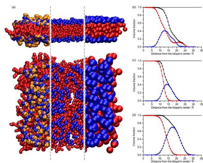
Figure 7: Mean field equilibrium ”snapshots” (set of most-probable conformations of the lipids) and the concentration profiles of tails (T, red lines), heads (H, blue lines) and the phospholipids (T+H, black lines) obtained with 44-, 10- and 3-beads models.

Similar calculations carried out for the 10-beads model show better reproducibility due to considerably reduced conformational space. In fact, 1 million of conformations is enough for calculations with different sampling to almost coincide in one curve with very small error bars (Figure 5). The absolute values of the free energy $f$ are shifted with respect to that of 44-units model, which is the consequence of different sizes of the units and the interactions parameters. However, the energy differences, the density profiles and the compressibility modulus are very close to that obtained with the previous model (Table 2). It is interesting to compare the energies of one and two layers in the box, red and green curves in Figure 5, correspondingly. The energies are quite similar at low densities of the layer and diverge significantly at high densities. This is consequence of the compression of the two layers due to lack of space in the box for two layers of equilibrium size. The energy per lipid corresponding to the maximal compression of two layers in the box coincides with the energy of a compressed layer. This fact reflects the consistency of our picture. On the other hand, high compression of a single layer, $A$ below $50$Ų, results in gradual splitting of the layer in two with smooth rearrangement of the lipid molecules. Some phospholipids flip and orient their “heads” in the center of the membrane. Thus, a single bilayer smoothly become broader and change its appearance to remind something between a single bilayer with a layer of heads in the center and two tightly compressed bilayers. This process is reflected in the flat part of the energy per lipid curve for $A$ below $50$Ų, where the distinction between one layer and two layers in the box can hardly be done.

The energy curve for the 3-beads model is presented in Figure 6. This is the simplest phospholipid model with only 3 beads, thus the conformational space is very limited and the results obtained with the sampling of 1 million of conformations represented here are close to these obtained with small sampling about 100-300 thousands. The difference between the energies of one and two layers in the box, noted for 10-beads model, is even more pronounced.

The mean field ”snapshots” of the most probable conformations of the layer in equilibrium and the corresponding density profiles for three models are presented in Figure 7. It shows how the coarse-graining and the decreasing of the model details influence the layer appearance. However, despite obvious differences in details caused by the differences in the molecule structures, the profiles looks quite similar, especially for the most coarse-grained 10- and 3-beads models. In case of the 44-units model, there is a small fraction of the hydrophobic T units at the surface, reflecting the structure of the phospholipid with some hydrophobic T groups in the head. Furthermore, different aspect ratio between T and H units in the models ($4:1$ in 10-beads and $2:1$ in the 3-beads model) lead to the corresponding difference in the relative density of T and H units. This correspondence is not valid for the 44-beads model, where the beads do overlap and some parts of the molecule are hidden from the solvent. The ratio between the areas under the T and H curves is $4.7:1$ which is different from the ratio between numbers of T and H beads in the molecule ($3.4:1$).

Finally few words should be said about the speed performance of three models. We run six series of calculations with different conformational sampling of 1-3 millions of conformations. The box is divided in $\sim 100$ parallel layers and the number of lipids in the box is varying from $300$ to $700$ with the step $10$. The program runs in parallel on 32-cores AMD machine with 128Gb of RAM. The most time consuming process is the solution of equations while the generation of the sampling at the beginning of calculation is relatively fast and almost does not affect the speed of calculation. In turn, the solution of the equations depends on the number of conformations in the sampling, the number of cells and the number of attempts to solve equations with different initial conditions. Since three models differ in the number of beads, implying different conformational space, the same accuracy of calculations in different models is achieved with different number of conformations in the sampling. The 44-beads model require several millions of conformations and 48 hours of calculations, the 10-beads model require one million of conformations and 17 hours, while the 3-beads model can get reliable results with a hundred thousands of conformations in few hours. Thus, the simplest 3-beads model is the fastest model which can reproduce the essential equilibrium properties of the phospholipid bilayer.

V Conclusions

In this work we report a computational tool providing relatively fast and stable solution of the equations of the SCMF theory in different geometries and different molecule structures. The SCMF theory is applied for the first time to model the DMPC phospholipid membranes with realistic thermodynamic properties. We show that all three coarse-grained models of phospholipids with the present parameters can adequately describe the equilibrium properties and the molecular structure of DMPC phospholipid bilayers in fluid phase. Among the essential properties of the phospholipid bilayers that correspond to the experimental data are the thickness of the membrane, the positions of different groups of the lipid in the bilayer, the compressibility of the membrane and the equilibrium interfacial area per lipid. The most detailed 44-beads model can reproduce the structure of the phospholipid layer with maximum details. The resulting density profiles of the groups of the phospholipid molecule can be used for the structural modeling in experimental techniques that require the molecular structure of the layer.

However, if one is interested in the average properties of the lipid bilayer, the simplest 3-beads model can be used to model the thermodynamics and the essential properties of self-assembled phospholipid bilayers. This model is faster and computationally more attractive than 44- and 10-beads models. Furthermore, we suggest that the 3-beads model with the parameters found in this work is used for simulation of more complex bilayer structures.

Appendix A Computational Details

Here we discuss the implementation details of the algorithm underlying the computational realization of the SCMF theory. The off-lattice realization of the program allows for conformations of the molecules in a real space. The algorithm consist of three independent parts: the generation of the sampling of conformations of molecules of any structure, the discretization of space according to the geometry of the problem and the solution of the SCMF equations (12). The independence of the parts insures the universality of the method which can be applied for molecules of any structure and their self-assembly in objects of any geometry.

A.1 Conformational sampling generation

First step is the generation of a representative set of conformations of a single molecule. This can be done with different techniques, including bead-to-bead chain growth or MC simulations. The conformations of a single molecule are generated once before solving the equations. They are stored in the RAM memory and not changed during the solution of equations, while the probabilities of each conformation are recalculated with the fields. This static memory allows for highly efficient parallelization of the program within the shared memory OpenMP platform, since the processors communicate very little between each other. The generation of conformations in the sampling is realized as follows:

1. Generation of a new conformation $\Gamma_{\alpha}$ of the molecule of type $\alpha$ with random position of the first bead inside the box. We set initial values of the conformation statistical weight $w_{\alpha}(\Gamma_{\alpha})=1$ and the intramolecular energy $H_{\alpha}^{intra}(\Gamma_{\alpha})=0$.

2. Iterative addition of new beads to the growing molecule and joining them one by one subject to self-avoidance condition. Depending on the final objective, one can use:

   1. Self-avoiding growth with the MC equilibration. The chain is generated as a self-avoiding off-lattice walk and the energy of interaction of the newly joined beads with the rest of the chain is accumulated in $H_{\alpha}^{intra}(\Gamma_{\alpha})$. The resulting chain is then equilibrated with MC crankshaft moves and reptations until the full equilibration of the configuration. In this case all conformations have the same statistical weight and $w_{\alpha}(\Gamma_{\alpha})=1$.

   2. Rosenbluth chain growth Rosenbluth and Rosenbluth (1955). A new bead is placed at a fixed distance from the previous bead either at random angle (freely joined chain) or with additional restrictions on the angles between the beads (chain with angle restrictions). Rosenbluth algorithm generates conformations with biased probability distribution. This bias is then calculated in the conformation weight and removed when the probabilities of each conformation are calculated. In order to calculate the Rosenbluth weight, one should try $N_{trial}$ times to place the new bead at a fixed distance from the previous bead and calculate the number $N_{allowed}$ of successful positions, allowed by self-avoidance condition. If $N_{allowed}>0$, a new position is accepted with the weight $1/N_{allowed}$, the energy of interaction is accumulated in $H_{\alpha}^{intra}(\Gamma_{\alpha})$ and the weight of the conformation $w_{\alpha}(\Gamma_{\alpha})$ is multiplied by the factor $1/N_{allowed}$. If there is no possibility to place the bead, $N_{allowed}=0$, the generation restarts from the beginning. The Rosenbluth algorithm is simple and efficient enough for generation of phospholipid molecules.

A.2 Discretization of space

Since the solution of equations of the SCMF theory in the integral form (12), (13) is not practical, the equations are simplified by the replacement of the integrals with the sums. The space is discretized according to the geometry of the system and the symmetry considerations. The integrals over the spatial coordinates, $d\boldsymbol{r}$, are replaced by the sums over auxiliary cells $i$ with the same values of the mean fields: $\left\langle c_{\beta}^{a}(\boldsymbol{r})\right\rangle=c_{\beta i}^{a}$ and $\lambda(\boldsymbol{r})=\lambda_{i}$. The discretization leads to the following approximate relations

$$\begin{split}\int u_{\alpha}^{a}(\Gamma_{\alpha},\boldsymbol{r})\left\langle c_{\beta}^{a}(\boldsymbol{r})\right\rangle d\boldsymbol{r}&\approx\sum_{i}c_{\beta i}^{a}\int_{i}u_{\alpha}^{a}(\Gamma_{\alpha},\boldsymbol{r})d\boldsymbol{r}\\ \int\lambda(\boldsymbol{r})\phi_{\alpha}(\Gamma_{\alpha},\boldsymbol{r})d\boldsymbol{r}&\approx\sum_{i}\lambda_{i}\int_{i}\phi_{\alpha}(\Gamma_{\alpha},\boldsymbol{r})d\boldsymbol{r}\end{split}$$ (20)

where $\sum_{i}$ denotes the sum over all auxiliary cells, while $\int_{i}$ is the integral over the $i$-th cell. Because of the structure of the equations, the integral over the single $i$-th cell can be evaluated once in the beginning of calculations, while the sums (20) are calculated during the solution of the equations. Although the number and the geometry of the cells can be arbitrary, their choice will restrict the geometry and the resolution of the resulting solutions. Thus, it is important to choose them accurately for a particular problem. In case of flat bilayers we choose a planar geometry with the cells parallel to the layer, thus we can only obtain the solutions that can lie in the layer.

The integrals over the conformational space of single molecules are replaced by the sums over the finite samplings generated in the first step

$$\phi_{\alpha i} = \sum_{\Gamma_{\alpha}}\phi_{\alpha i}(\Gamma_{\alpha})\rho_{\alpha}(\Gamma_{\alpha}),$$ (21)

$$c_{\alpha i}^{a} = \sum_{\Gamma_{\alpha}}c_{\alpha i}^{a}(\Gamma_{\alpha})\rho_{\alpha}(\Gamma_{\alpha})\quad$$

where the mean field volume fraction $\phi_{\alpha i}$ and the mean field concentration $c_{\alpha i}^{a}$ of $a$-beads of the molecule of type $\alpha$ in the cell $i$ are related to the corresponding volume fraction $\phi_{\alpha i}(\Gamma_{\alpha})$ and the concentration $c_{\alpha i}^{a}(\Gamma_{\alpha})$ of the conformation $\Gamma_{\alpha}$.

The integral expression (11) for the $\rho_{\alpha}(\Gamma_{\alpha})$ yields in form

$$\begin{split}\rho_{\alpha}(\Gamma_{\alpha})&=\frac{1}{Z_{\alpha}w_{\alpha}(\Gamma_{\alpha})}\exp\left(-H_{\alpha}^{intra}(\Gamma_{\alpha})-\right.\\ &\sum_{\beta=1}^{M}(N_{\beta}-\delta_{\alpha\beta})\times\\ &\left.\times\sum_{ai}\epsilon_{\alpha i}^{a}(\Gamma_{\alpha})c_{\beta i}^{a}+\sum_{i}\lambda_{i}v_{\alpha i}(\Gamma_{\alpha})\right)\end{split}$$ (22)

where $w_{\alpha}(\Gamma_{\alpha})$ is the Rosenbluth weight calculated during the generation of the chains, and the constant $Z_{\alpha}$ insures the normalization of the probability $\sum_{\Gamma_{\alpha}}\rho_{\alpha}(\Gamma_{\alpha})=1$.

The expression for probabilities (22) is accompanied with the following relations

$$\begin{split}v_{s}\lambda_{i}&\approx\ln\phi_{si}+\sum_{\beta=1}^{M}(N_{\beta}-\delta_{s\beta})\sum_{a}\epsilon_{si}^{a}c_{\beta i}^{a},\\ &\quad\phi_{si}=\phi_{0}-\sum_{\alpha=1,\alpha\neq s}^{M}N_{\alpha}\phi_{\alpha i}\\ \epsilon_{\alpha i}^{a}(\Gamma_{\alpha})&=\int_{i}u_{\alpha}^{a}(\Gamma_{\alpha},\boldsymbol{r})d\boldsymbol{r},\\ &\quad v_{\alpha i}(\Gamma_{\alpha})=V_{i}\phi_{\alpha i}(\Gamma_{\alpha})=\int_{i}\phi_{\alpha}(\Gamma_{\alpha},\boldsymbol{r})d\boldsymbol{r}\end{split}$$ (23)

The quantities $v_{\alpha i}(\Gamma_{\alpha})$, $\epsilon_{\alpha i}^{a}(\Gamma_{\alpha})$ and $c_{\alpha i}^{a}(\Gamma_{\alpha})$ are calculated using the MC integration technique. The volumes $v_{\alpha i}(\Gamma_{\alpha})$ are calculated as follows: one throws randomly $N_{trials}$ points inside the volume occupied by the bead and determine the cell where each of these points hits. Each point contributes to the volume in the cell with the value $v_{a}/\left(N_{trials}N_{int}\right)$, where $N_{int}$ is the number of the beads hit by the point and $v_{a}$ is the volume of the bead. The volume fractions $\phi_{\alpha i}(\Gamma_{\alpha})$ are related to the volumes $v_{\alpha i}(\Gamma_{\alpha})$ as $\phi_{\alpha i}(\Gamma_{\alpha})=v_{\alpha i}(\Gamma_{\alpha})/V_{i}$, where $V_{i}$ is the volume of the $i$-th auxiliary cell. The concentrations $c_{\alpha i}^{a}(\Gamma_{\alpha})$ are calculated similarly, except that each random point contributes to $c_{\alpha i}^{a}(\Gamma_{\alpha})$ with the value $1/N_{trials}$. The interaction energies $\epsilon_{\alpha i}^{a}(\Gamma_{\alpha})$ are calculated with the help of the $N_{trials}$ points thrown for every $a$ at a distance $r$ from the center of the bead $b$ such that $r_{min}<r<r_{max}$, where $r_{min}$ is the minimum distance at which the bead of type $a$ can approach to the $b$ bead, and $r_{max}$ is the maximum distance at which the interaction potential acting between $a$ and $b$ beads is non-zero. If the bead of type $a$ in the position of the trial point does not have any intersection with the beads of the chain, its contribution to the $\epsilon_{\alpha i}^{a}(\Gamma_{\alpha})$ is $\frac{4}{3}\pi\left(r_{max}^{3}-r_{min}^{3}\right)U^{ab}(r)/N_{trials}$, where $i$ is the number of the auxiliary cell where the trial point hits, and $U^{ab}(r)$ is the pair potential acting between the beads of types $a$ and $b$. Since the solvent is implicit in our model, the quantities $\epsilon_{si}^{a}$ describing the interaction between the solvent and the bead of type $a$ have to be treated separately. We evaluate them by a simple approximate expression

$$\epsilon_{si}^{a}\approx\frac{4}{3}\pi(r_{sa}^{3}-(r_{s}+r_{a})^{3})\varepsilon_{sa}$$ (24)

where we assume the square well potentials between the solvent molecules $s$ and the beads $a$ with energy $\varepsilon_{sa}$ at the distance closer than $r_{sa}$. Here the radius of solvent is $r_{s}$ and the radius of the $a$ bead is $r_{a}$.

It is noteworthy that the incorporation of the Rosenbluth weight $w_{\alpha}(\Gamma_{\alpha})$ into the expression for probabilities (22) may lead to confusion. Although most of the averages can be calculated with the expressions similar to (21), the averages of expressions containing explicitly the probability $\rho_{\alpha}$ should be treated separately. For example, the entropy term in the free energy (10) leads to the additional term when we replace the integral with the sum

$$N_{\alpha}\left\langle\ln{\frac{\rho_{\alpha}N_{\alpha}}{e}\Lambda_{\alpha}}\right\rangle=N_{\alpha}\sum_{\Gamma_{\alpha}}\rho_{\alpha}(\Gamma_{\alpha})\ln{\frac{\rho_{\alpha}(\Gamma_{\alpha})N_{\alpha}}{e}\Lambda_{\alpha}}+$$

$$N_{\alpha}\sum_{\Gamma_{\alpha}}\rho_{\alpha}(\Gamma_{\alpha})\ln{w_{\alpha}(\Gamma_{\alpha})\varkappa_{\alpha}}$$ (25)

where $\varkappa_{\alpha}$ is the number of conformations in the sampling of the molecule of type $\alpha$.

The expressions (21), (22) and (23) form a closed set of algebraical equations with respect to variables $\phi_{\alpha i}$ and $c_{\alpha i}^{a}$ which can be solved numerically. We must admit however, that the solution of these non-linear equations is not a straightforward task.

A.3 Numerical implemetation

In this work we have implemented the SCMF theory in C++. The program is based on Newton-Rapson technique which provides the efficient and stable solution of the SCMF equations. It has a modular structure which makes it very flexible for modification, further development and extension for new applications.

The first module is the sampling generator, which generates the molecules conformations and calculates the volumes and interactions according to the Appendix A.1. The code for generation of molecules with different structures can be added to this module or changed independently from other parts of the program.

The second module specify the geometry of the problem: 1D spherical, 1D planar, 2D planar, 2D cylindrical, or 3D cubic. It contains the description of the geometry and divide the simulation box into set of auxiliary cells. The modification of this part of code provides an easy way to implement different types of the system geometry. It is worth to note here one technical improvement that significantly increase the performance of the calculations. Since the molecules have small size compared to the size of the box, their contribution to most of the auxiliary cells is zero, thus matrices $\epsilon_{\alpha i}^{a}(\Gamma_{\alpha})$, $c_{\alpha i}^{a}(\Gamma_{\alpha})$ and $v_{\alpha i}(\Gamma_{\alpha})$ have many zero values. In this second module of the program the simple compression of these data is realized via elimination of zeros from these matrices. This helps to save computer memory and, on the next step, speed up the calculations by elimination of the sums over the cells containing zeros.

The core of the third module is the modified Newton-Rapson solver for the solution of SCMF equations. It involves the iterative solver which calculates on each step the matrix of analytical derivatives of equations 21 with respect to unknown variables along with the analytical expressions including the sums over the conformational samplings. The next approximation of the solution is determined by the inversion of this matrix until the required accuracy is reached. To avoid occasional instability of the Newton-Rapson scheme, the algorithm artificially restrains too big steps which may drop the next approximation outside a reasonable range. The algorithm is able to find several solutions simultaneously by repeating the calculations several times with different initial conditions.

References

- Lipowsky and Sackmann (1995) R. Lipowsky and E. Sackmann, Structure and Dynamics of Membranes, Elsevier, Amsterdam, 1995.
- Muller et al. (2006) M. Muller, K. Katsov and M. Schick, Physics Reports, 2006, 434, 113–176.
- Venturolia et al. (2006) M. Venturolia, M. M. Sperottob, M. Kranenburgc and B. Smit, Physics Reports, 2006, 437, 1–54.
- Tieleman et al. (1997) D. Tieleman, S. Marrink and H. Berendsen, Biochimica et Biophysica Acta, 1997, 1331, 235–270.
- Damodaran et al. (1992) K. V. Damodaran, K. M. Merz and B. P. Gaber, Biochemistry, 1992, 31, 7656.
- Damodaran and Merz (1994) K. V. Damodaran and K. M. Merz, Biophysical Journal, 1994, 66, 1076–1087.
- Smondyrev and Berkowitz (1999) A. M. Smondyrev and M. L. Berkowitz, Journal of Computational Chemistry, 1999, 20, 531–545.
- Robinson et al. (1994) A. J. Robinson, W. G. Richards, P. J. Thomas and M. M. Hann, Biophysical Journal, 1994, 87, 2345–2354.
- Heller et al. (1993) H. Heller, M. Schafer and K. Schulten, J. Phys. Chem., 1993, 97, 8343.
- Tuckerman et al. (1992) M. Tuckerman, B. Berne and G. Martyna, J. Chem. Phys., 1992, 97, 1990.
- Lyubartsev (2005) A. P. Lyubartsev, Eur Biophys J, 2005, 35, 53–61.
- Hyvonen et al. (1997) M. T. Hyvonen, T. T. Rantala and M. Ala-Korpela, Biophysical Journal, 1997, 73, 2907–2923.
- Kotelyanskii and Theodorou (2004) M. Kotelyanskii and D. N. Theodorou, Simulation Methods for Polymers, CRC Press, 2004.
- Goetz and Lipowsky (1998) R. Goetz and R. Lipowsky, J. Chem. Phys., 1998, 108, 7397–7409.
- Shelley et al. (2001) J. C. Shelley, M. Y. Shelley, R. C. Reeder, S. Bandyopadhyay and M. L. Klein, J. Phys. Chem. B, 2001, 105, 4464–4470.
- Shelley et al. (2001) J. C. Shelley, M. Y. Shelley, R. C. Reeder, S. Bandyopadhyay, P. B. Moore and M. L. Klein, J. Phys. Chem. B, 2001, 105, 9785–9792.
- Muller et al. (2003) M. Muller, K. Katsov and M. Schick, J. Polym. Sci. B: Polym. Phys., 2003, 41, 1441 1450.
- Marrink et al. (2004) S. Marrink, A. de Vries and A. Mark, J. Phys. Chem. B, 2004, 108, 750.
- Cooke et al. (2005) I. R. Cooke, K. Kremer and M. Deserno, Phys. Rev. E, 2005, 72, 011506.
- Ben-Shaul et al. (1985) A. Ben-Shaul, I. Szleifer and W. M. Gelbart, J. Chem. Phys., 1985, 83, 3597.
- Ben-Shaul et al. (1986) A. Ben-Shaul, I. Szleifer and W. M. Gelbart, J. Chem. Pys., 1986, 85, 5345.
- Mackie et al. (1997) A. D. Mackie, A. Z. Panagiotopoulos and I. Szleifer, Langmuir, 1997, 13, 5022.
- Al-Anber et al. (2005) Z. A. Al-Anber, J. Bonet-Avalos and A. D. Mackie, J. Chem. Phys., 2005, 122, 104910.
- Al-Anber et al. (2003) Z. A. Al-Anber, J. Bonet-Avalos, M. A. Floriano and A. D. Mackie, J. Chem. Phys., 2003, 118, 3816–3826.
- Shvartzman-Cohen et al. (2009) R. Shvartzman-Cohen, C. Ren, I. Szleifer and R. Yerushalmi-Rozen, Soft Matter, 2009, 5, 5003–5011.
- Altevogt et al. (1999) P. Altevogt, O. Evers, J. Fraaije, N. Maurits and B. van Vlimmeren, J. of Mol. Struct. (Theochem), 1999, 463, 139–143.
- Fraaije et al. (1997) J. G. E. M. Fraaije, B. A. C. van Vlimmeren, N. M. Maurits, M. Postma, O. A. Evers, C. Hoffmann, P. Altevogt and G. Goldbeck-Wood, J. Chem. Phys., 1997, 106, 4260–4269.
- Doi (2003) M. Doi, Pure Appl. Chem., 2003, 75, 1395–1402.
- Soldera et al. (2009) A. Soldera, Y. Qi and W. T. Capehart, J. Chem. Phys., 2009, 130, 064902.
- Mae et al. (2008) H. Mae, M. Omiya and K. Kishimoto, J. Solid Mech. and Mat. Eng., 2008, 2, 1018–1036.
- Muller and Smith (2005) M. Muller and G. D. Smith, Journal of Polymer Science: Part B: Polymer Physics, 2005, 43, 934 958.
- Daoulas et al. (2006) K. C. Daoulas, M. Muller, J. J. de Pablo, P. F. Nealey and G. D. Smith, Soft Matter, 2006, 2, 573–583.
- Daoulas and Muller (2006) K. C. Daoulas and M. Muller, J. Chem. Phys., 2006, 125, 184904.
- Marcelja (1973) S. Marcelja, Nature, 1973, 241, 451–453.
- Marcelja (1974) S. Marcelja, Biochem. Biophys. Acta, 1974, 367, 165–176.
- Rosenbluth and Rosenbluth (1955) M. N. Rosenbluth and A. Rosenbluth, J. Chem. Phys., 1955, 23, 356.
- Frenkel and Smit (2002) D. Frenkel and B. Smit, Understanding molecular simulation: from algorithms to applications, Academic Press, 2002.
- Kucerka et al. (2005) N. Kucerka, Y. Liu, N. Chu, H. I. Petrache, S. Tristram-Nagle and J. F. Nagle, Biophysical Journal, 2005, 88, 2626–2637.
- Nagle and Tristram-Nagle (2000) J. F. Nagle and S. Tristram-Nagle, Biochimica et Biophysica Acta, 2000, 1469, 159–195.
- Mathai et al. (2008) J. C. Mathai, S. Tristram-Nagle, J. F. Nagle and M. L. Zeidel, The Journal of General Physiology, 2008, 131, 69–76.
- Koynova and Caffrey (1998) R. Koynova and M. Caffrey, Biochimica et Biophysica Acta, 1998, 1376, 91–145.