Wannier-function approach to spin excitations in solids

Abstract

We present a computational scheme to study spin excitations in magnetic materials from first principles. The central quantity is the transverse spin susceptibility, from which the complete excitation spectrum, including single-particle spin-flip Stoner excitations and collective spin-wave modes, can be obtained. The susceptibility is derived from many-body perturbation theory and includes dynamic correlation through a summation over ladder diagrams that describe the coupling of electrons and holes with opposite spins. In contrast to earlier studies, we do not use a model potential with adjustable parameters for the electron-hole interaction but employ the random-phase approximation. To reduce the numerical cost for the calculation of the four-point scattering matrix we perform a projection onto maximally localized Wannier functions, which allows us to truncate the matrix efficiently by exploiting the short spatial range of electronic correlation in the partially filled d or f orbitals. Our implementation is based on the full-potential linearized augmented-plane-wave (FLAPW) method. Starting from a ground-state calculation within the local-spin-density approximation (LSDA), we first analyze the matrix elements of the screened Coulomb potential in the Wannier basis for the 3d transition-metal series. In particular, we discuss the differences between a constrained nonmagnetic and a proper spin-polarized treatment for the ferromagnets Fe, Co, and Ni. The spectrum of single-particle and collective spin excitations in fcc Ni is then studied in detail. The calculated spin-wave dispersion is in good overall agreement with experimental data and contains both an acoustic and an optical branch for intermediate wave vectors along the $[1\,0\,0]$ direction. In addition, we find evidence for a similar double-peak structure in the spectral function along the $[1\,1\,1]$ direction. To investigate the influence of static correlation we finally consider LSDA+$U$ as an alternative starting point and show that, together with an improved description of the Fermi surface, it yields a more accurate quantitative value for the spin-wave stiffness constant, which is overestimated in the LSDA.

I introduction

Spin excitations in solids are of fundamental interest for a wide variety of phenomena. For example, in magnetic materials at low temperatures collective spin excitations, so-called spin waves or magnons,Moriya leave a mark on the transport, dynamical, and thermodynamical properties. The spin waves contribute to the specific heat with a $T^{3/2}$ term in addition to the $T^{3}$ term from phonon excitations. The low-temperature behavior of the magnetization in three-dimensional magnetic solids is also dominated by spin-wave excitations: In ferromagnets the magnetization drops as $T^{3/2}$, while the sublattice magnetization in antiferromagnets obeys a $T^{2}$ law.Kobler In low-dimensional systems spin-wave excitations even destroy the long-range magnetic order completely at any finite temperature $T$ in the absence of a magnetic anisotropy.Mermin As the temperature increases, additional single-particle spin-flip processes, the so-called Stoner excitations, take place, which further contribute to the temperature variation of the magnetization and cause a damping of the spin-wave modes. Spin waves can also couple to charge excitations around the Fermi level. Such interactions lead to a pronounced energy renormalization in the quasiparticle band dispersion,Hofmann:09 or control the spin-dependent inelastic mean free path of hot electrons in ferromagnets.Hong_1 ; Hong_2 ; Zhukov_1 ; Zhukov_2 Another interesting phenomenon is high-temperature superconductivity, in which spin waves have been proposed as a possible mediator for the attractive electron-electron interaction.Dagotto ; Scalapino This scenario was recently confirmed by infrared spectroscopy and neutron scattering measurements for the high-temperature superconductor YBa₂Cu₃O_6.92.Carbotte ; Dahm

Spin excitations in solids are also of central interest in the field of spintronics. The writing process of magnetic information in a giant magneto resistance or tunnel magneto resistance device is closely related to the rotation of the magnetization, a process generating and radiating spin waves at all wave lengths, whose damping rate is an important parameter determining the writing time.Choi Spin waves are also generated during the reading process, as hot electrons impinge at the interfaces between the insulating barrier and the magnetic electrodes of magnetic tunnel junctions, which causes a reduction of the magneto resistance.Farle

The properties and physics of spin waves evidently comprise an unusually rich area of research. A lot of information about the spin dynamics in solids can be obtained from the magnetic response function (or dynamical spin susceptibility). The spectrum of magnetic excitations corresponds to the poles of the response function and can be directly compared with experiments like inelastic neutron scattering. In this way it provides insight into the nature of the exchange coupling and the complex magnetic order. The magnetic response function is thus a central quantity for the theoretical description of magnetic materials.

So far most theoretical studies of magnetic excitations in solids were based on an adiabatic treatment of the spin degrees of freedom in which the slow motion of the magnetic moments and the fast motion of the electrons are separated by mapping the complex itinerant electron problem onto the classical Heisenberg Hamiltonian with exchange parameters obtained from constrained density-functional theory (DFT) calculations.Kubler ; Sandratskii ; Nordstrom ; Johansson ; Halilov ; Schilfgaarde ; Fahnle ; Pajda Within this approach the spin-wave excitations can be calculated efficiently, whereas the single-particle Stoner excitations are neglected. Furthermore, the spin-wave life times are not accessible. From a fundamental point of view, the Heisenberg model is justified only for local-moment systems like insulators and rare earths, which possess well-defined spin-wave modes over the entire Brillouin zone, so that the adiabatic approximation is reliable. For itinerant-electron magnets the adiabatic approximation yields reasonable results only in the long-wave-length region, i.e., for small wave vectors. For short wave lengths the discrepancy with experiments can be large, however. For example, the multiple branches in the spin-wave dispersion of 3d ferromagnets cannot be captured.Cooke_1 ; Cooke_2

First-principles calculations of the magnetic response function using realistic energy bands and wave functions are very rare. Initial attempts by Cooke et al.Cooke_1 ; Cooke_2 ; Cooke_3 ; Cooke_4 within the framework of many-body perturbation theory (MBPT) were based on a tight-binding description of the electronic energy bands. These authors studied the spin-wave dispersion of 3d ferromagnets and obtained reasonable agreement with experiments; in particular, the optical branch in the spin-wave dispersion of fcc Ni was correctly described.Cooke_3 Using a similar approach, Mills and co-workersMills_1 ; Mills_2 ; Mills_3 ; Mills_4 carried out extensive calculations to explore the spin dynamics in ultrathin ferromagnetic films on nonmagnetic substrates. Recently more realistic treatments of the spin-wave spectra in 3d ferromagnets were reported by SavrasovSavrasov_SW and Buczek et al.Pavel within time-dependent density-functional theory (TDDFT) and by Karlsson and Aryasetiawan within MBPT.Karlsson_1 However, in the latter work the authors used a simplified model potential with an adjustable parameter to estimate the matrix elements of the screened Coulomb interaction. Under these circumstances both TDDFT and MBPT appear to give similar results for the spin-wave dispersions of Fe and Ni. The results for Fe are in good agreement with available experimental data, while for Ni the optical branch is too high in energy, which was attributed to the overestimation of the exchange splitting of Ni within the underlying LSDA.Karlsson_1

The aim of the present work is to develop a practical computational scheme to study excitation spectra of magnetic materials from first principles. The magnetic response function is calculated within a many-body context following the formalism given in Ref. Aryasetiawan, . To study collective spin-wave excitations we include vertex corrections in the form of ladder diagrams, which describe the coupling of electrons and holes with opposite spins via the screened Coulomb interaction. In analogy to the $T$-matrix that describes the particle-particle scattering channel, here we use the same term for the electron-hole channel in agreement with the definition of Strinati.Strinati In contrast to earlier treatments, the matrix elements of the screened Coulomb potential are calculated entirely from first principles. In order to reduce the numerical cost for the calculation of the four-point $T$-matrix we exploit a transformation to maximally localized Wannier functions (MLWFs), which provide a more efficient basis to study local correlations than extended Bloch states.Wannier_1 ; Wannier_2 ; Wannier_3 ; Wannier_4 ; Wannier_5 ; Wannier_6 ; Wannier_7 ; LC_1 ; LC_2 ; LC_3 ; LC_4 This use of localized orbitals makes our scheme very efficient for complex magnetic materials with many atoms per unit cell. Our implementation is based on the FLAPW method. In the following we first calculate the matrix elements of the Coulomb potential for the 3d transition-metal series in the Wannier basis and perform extensive convergence tests. The magnetic excitations in fcc Ni are then studied in detail based on the LSDA and LSDA+$U$ methods. We find that both approaches yield qualitatively similar results for the spin-wave spectra and overall dispersion. However, the static correlation effects seem to be important for the spin-wave stiffness constant, which is overestimated within LSDA. In contrast to some previous theoretical studies,Cooke_3 ; Karlsson_1 our calculations clearly indicate the existence of an optical branch in the spin-wave dispersion curve of Ni along the $[1\,1\,1]$ in addition to that along the $[1\,0\,0]$ direction in the Brillouin zone. In general, the obtained results are in good agreement with available experimental data.

This paper is organized as follows. In Sec. II we describe the computational method. Section III contains the results for the matrix elements of the screened Coulomb potential for the 3d transition metals. In Sec. IV we present results for the magnetic excitations in fcc Ni together with a detailed discussion. In Sec. V we summarize our conclusions and give an outlook. Unless otherwise indicated, Hartree atomic units are used throughout.

II Computational Method

II.1 Magnetic response function

The time-ordered magnetic response function (or dynamical spin susceptibility) is given in real space by the correlation function

$$R^{ij}(1,2)=-i\langle\mathcal{T}[\hat{\sigma}^{i}(1),\hat{\sigma}^{j}(2)]\rangle\>,$$ (1)

where $\mathcal{T}$ is the time-ordering operator and $\hat{\sigma}^{i}(1)$ are the spin-density operators with $i\in\{x,y,z,-,+\}$, where $-$ and $+$ correspond to the spin annihilation ($\hat{\sigma}^{-}=\hat{\sigma}^{x}-i\hat{\sigma}^{y}$) and creation ($\hat{\sigma}^{+}=\hat{\sigma}^{x}+i\hat{\sigma}^{y}$) operator, respectively. For simplicity we use the short-hand notation $1=(\mathbf{r}_{1},t_{1})$. The expectation value of $\hat{\sigma}^{i}(1)$ with respect to the many-body ground state is given by

$$\langle\hat{\sigma}^{i}(1)\rangle=-i\sum_{\alpha,\beta}\sigma^{i}_{\beta\alpha}G_{\alpha\beta}(1,1^{+})$$ (2)

with the Pauli spin matrices $\sigma^{i}$, the single-particle Green function $G$, and the spin indices $\alpha$ and $\beta$. The notation $1^{+}$ indicates that the time variable is increased by an infinitesimal to ensure the proper time ordering $t_{1}^{+}>t_{1}$. The magnetic response function can be obtained from the spin density by the functional derivative

$$R^{ij}(1,2)=\frac{\delta\langle\hat{\sigma}^{i}(1)\rangle}{\delta B_{j}(2)}\>,$$ (3)

where $i$ and $j$ correspond to the components of the magnetization and the magnetic-field vector, respectively. The latter incorporates a factor $g\mu_{\mathrm{B}}/2$, where the $\mu_{\mathrm{B}}$ denotes the Bohr magneton and $g$ the electron $g$-factor, so that the Zeeman term in the Hamiltonian operator takes the form $+\mathbf{B}\cdot\mathbf{\sigma}$.

II.2 $T$-matrix approximation

The single-particle Green function in Eq. (2) is given by the Dyson equation

$$G_{\alpha\beta}(1,2) = G^{0}_{\alpha}(1,2)\delta_{\alpha\beta}+\sum_{\gamma}\iint G^{0}_{\alpha}(1,3)$$ (4)

$$\times\Sigma_{\alpha\gamma}(3,4)G_{\gamma\beta}(4,2)\>d3\>d4\>,$$

where $G^{0}$ is the spin-diagonal Green function of the noninteracting Hartree system and $\Sigma$ the nonlocal dynamic self-energy, which incorporates all exchange-correlation effects. With the identity

$$\frac{\delta G_{\alpha\beta}(1,3)}{\delta B_{j}(2)}$$ (5)

$$=-\sum_{\gamma,\delta}\iint G_{\alpha\gamma}(1,4)\frac{\delta G^{-1}_{\gamma\delta}(4,5)}{\delta B_{j}(2)}G_{\delta\beta}(5,3)\>d4\>d5$$

one can rewrite the magnetic response function (3) as

$$R^{ij}(1,2)$$ (6)

$$= -i\sum_{\alpha,\beta,\gamma,\delta}\sigma^{i}_{\beta\alpha}\iint G_{\alpha\gamma}(1,3)\bigg{[}\sigma^{j}_{\gamma\delta}\delta(2-3)$$

$$\times\delta(3-4)+\frac{\delta\Sigma_{\gamma\delta}(3,4)}{\delta B_{j}(2)}\bigg{]}G_{\delta\beta}(4,1^{+})\>d3\>d4\>.$$

In this work we use the $GW$ approximation for the self-energyHedin

$$\Sigma_{\gamma\delta}(3,4)=iG_{\gamma\delta}(3,4)W(3,4)\>.$$ (7)

The functional derivative of the self-energy with respect to the external magnetic field is then given by

$$\frac{\delta\Sigma_{\gamma\delta}(3,4)}{\delta B_{j}(2)} = i\frac{\delta G_{\gamma\delta}(3,4)}{\delta B_{j}(2)}W(3,4)+iG_{\gamma\delta}(3,4)$$ (8)

$$\times\frac{\delta W(3,4)}{\delta B_{j}(2)}\>.$$

For systems with a collinear magnetic ground state only the first term on the right-hand side yields a nonzero contribution to the magnetic response function.Aryasetiawan Furthermore, in this case the Green function is diagonal in spin space and can be written as $G_{\alpha\beta}(1,2)=G_{\alpha}(1,2)\delta_{\alpha\beta}$. The dynamically screened Coulomb potential $W(3,4)$ is given by

$$W(3,4)=v(3,4)+\iint v(3,5)P(5,6)W(6,4)\>d5\>d6\>,$$ (9)

where $v(3,4)=\delta(t_{3}-t_{4})/|\mathbf{r}_{3}-\mathbf{r}_{4}|$ is the bare Coulomb potential and $P(5,6)$ the polarizability in the random-phase approximation (RPA). The latter is expressed by

$$P(5,6)=-\sum_{\alpha}K^{\alpha\alpha}(5,6;6,5)\>,$$ (10)

where the kernel $K$ is defined as

$$K^{\alpha\beta}(1,3;4,2)=iG_{\alpha}(1,3)G_{\beta}(4,2^{+})\>.$$ (11)

After collecting all terms we obtain

$$R^{ij}(1,2) = -\sum_{\alpha,\beta}\sigma^{i}_{\beta\alpha}\sigma^{j}_{\alpha\beta}\big{[}K^{\alpha\beta}(1,2;2,1)$$ (12)

$$+L^{\alpha\beta}(1,2;2,1)\big{]}$$

for the magnetic response function. The second contribution is given by

$$L^{\alpha\beta}(1,2;2,1) = \iiiint K^{\alpha\beta}(1,3;4,1)T^{\alpha\beta}(3,5;6,4)$$ (13)

$$\times K^{\alpha\beta}(5,2;2,6)\>d3\>d4\>d5\>d6\>,$$

where the $T$-matrix obeys the Bethe-Salpeter equation

$$T^{\alpha\beta}(1,3;4,2)$$ (14)

$$= W(1,2)\delta(1-3)\delta(2-4)+W(1,2)$$

$$\times\iint K^{\alpha\beta}(1,5;6,2)T^{\alpha\beta}(5,3;4,6)\>d5\>d6\>.$$

The first term in Eq. (12) represents the response of the noninteracting system, i.e., the Kohn-Sham spin susceptibility. The second term contains the $T$-matrix, which describes dynamic correlation in the form of repeated scattering events of particle-hole pairs with opposite spins and is responsible for the occurrence of collective spin-wave excitations. The Feynman diagrams for the magnetic response function $R$ and the $T$-matrix are displayed in Fig. 1.

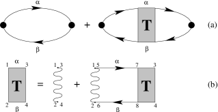
Figure 1: Diagrammatic representation of (a) the magnetic response function and (b) the $T$-matrix.

For a practical evaluation of the magnetic response function we replace the full renormalized Green function $G_{\alpha}(1,2)$ by an appropriate mean-field approximation (LSDA, LSDA+$U$, etc.). Moreover, we employ an instantaneous interaction of the form $W(\mathbf{r}_{1},\mathbf{r}_{2};t_{1}-t_{2})\approx W(\mathbf{r}_{1},\mathbf{r}_{2})\,\delta(t_{1}-t_{2})$ with $W(\mathbf{r}_{1},\mathbf{r}_{2})=\int_{-\infty}^{\infty}W(\mathbf{r}_{1},\mathbf{r}_{2};\tau)\,d\tau$ in Eq. (14). This is justified by the observation that the matrix elements of $W(\mathbf{r}_{1},\mathbf{r}_{2})$ do not vary strongly in the low-frequency region ($\omega<1$ eV), in which the spin-wave excitations occur.Jepsen ; Miyake Under these circumstances it is sufficient to calculate the kernel (11) for $t_{2}=t_{1}$ and $t_{4}=t_{3}$. In fact, due to time translation symmetry the resulting expression depends only on the difference $t_{1}-t_{3}$ and is given by the Fourier transform of

$$K^{\alpha\beta}(\textbf{r}_{1},\textbf{r}_{3};\textbf{r}_{4},\textbf{r}_{2};\omega)$$ (15)

$$= \sum_{\mathbf{k},m}^{\textmd{occ}}\sum_{\mathbf{k}^{\prime},m^{\prime}}^{\textmd{unocc}}\bigg{(}\frac{\varphi_{\mathbf{k}m}^{\alpha}(\textbf{r}_{1})\varphi_{\mathbf{k}m}^{\alpha*}(\textbf{r}_{3})\varphi_{\mathbf{k}^{\prime}m^{\prime}}^{\beta}(\textbf{r}_{4})\varphi_{\mathbf{k}^{\prime}m^{\prime}}^{\beta*}(\textbf{r}_{2})}{\omega+(\epsilon_{\mathbf{k}^{\prime}m^{\prime}}^{\beta}-\epsilon_{\mathbf{k}m}^{\alpha})-i\delta}$$

$$-\frac{\varphi_{\mathbf{k}^{\prime}m^{\prime}}^{\alpha}(\textbf{r}_{1})\varphi_{\mathbf{k}^{\prime}m^{\prime}}^{\alpha*}(\textbf{r}_{3})\varphi_{\mathbf{k}m}^{\beta}(\textbf{r}_{4})\varphi_{\mathbf{k}m}^{\beta*}(\textbf{r}_{2})}{\omega-(\epsilon_{\mathbf{k}^{\prime}m^{\prime}}^{\alpha}-\epsilon_{\mathbf{k}m}^{\beta})+i\delta}\bigg{)}\>,$$

where $\varphi_{\mathbf{k}m}^{\alpha}(\textbf{r})$ and $\epsilon_{\mathbf{k}m}^{\alpha}$ are the LSDA (LSDA+$U$) eigenstates and eigenvalues, respectively.

II.3 Implementation in the Wannier basis

In order to reduce the numerical cost for the calculation of the four-point kernel $K$ we exploit a transformation to maximally localized Wannier functions, which allows us to efficiently truncate the matrix in real space. The generalized Wannier functions $w_{n\textbf{R}}^{\alpha}(\textbf{r})$ with orbital index $n$ and spin $\alpha$ at the site R are defined as Fourier transforms of the Bloch states $\varphi_{\mathbf{k}m}^{\alpha}(\textbf{r})$ according to

$$w_{n\textbf{R}}^{\alpha}(\textbf{r}) = \frac{1}{N}\sum_{\mathbf{k}}e^{-i\mathbf{k}\cdot\textbf{R}}\sum_{m}U_{mn}^{\alpha(\mathbf{k})}\varphi_{\mathbf{k}m}^{\alpha}(\textbf{r})$$ (16)

$$= \frac{1}{N}\sum_{\mathbf{k}}e^{-i\mathbf{k}\cdot\textbf{R}}w_{\mathbf{k}n}^{\alpha}(\textbf{r})\>,$$

where $N$ is the number of discrete $\mathbf{k}$ points in the full Brillouin zone and $U_{mn}^{\alpha(\mathbf{k})}$ denote the transformation matrices. The latter are determined by minimizing the spread

$$\Omega=\sum_{n,\alpha}\big{(}\langle w_{n\mathbf{0}}^{\alpha}|r^{2}|w_{n\mathbf{0}}^{\alpha}\rangle-\langle w_{n\mathbf{0}}^{\alpha}|\textbf{r}|w_{n\mathbf{0}}^{\alpha}\rangle^{2}\big{)}\>,$$ (17)

where the sum runs over all Wannier functions. We employ the algorithm for minimizing the spread initially proposed by Marzari and VanderbiltWannier_1 for isolated groups of bands and later extended to entangled energy bands.Wannier_2

The matrix elements of the screened Coulomb potential in the MLWF basis are given by

$$W^{\alpha\beta}_{n_{1}\textbf{R}_{1}n_{3}\textbf{R}_{3};n_{4}\textbf{R}_{4}n_{2}\textbf{R}_{2}}$$ (18)

$$= \iint w_{n_{1}\textbf{R}_{1}}^{\alpha*}(\textbf{r})w_{n_{3}\textbf{R}_{3}}^{\alpha}(\textbf{r})W(\textbf{r},\textbf{r}^{\prime})$$

$$\times w_{n_{4}\textbf{R}_{4}}^{\beta*}(\textbf{r}^{\prime})w_{n_{2}\textbf{R}_{2}}^{\beta}(\textbf{r}^{\prime})\>d^{3}r\>d^{3}r^{\prime}\>.$$

The screened potential $W(\textbf{r},\textbf{r}^{\prime})$ itself is calculated within the RPA using the mixed product basis.Mixed_Basis ; Mixed_Basis_2 ; Friedrich As we use only the on-site matrix elements of $W$, we set $\textbf{R}_{1}=\textbf{R}_{2}=\textbf{R}_{2}=\textbf{R}_{4}$ and eventually obtain

$$W^{\alpha\beta}_{n_{1}n_{3};n_{4}n_{2}}$$ (19)

$$= \frac{1}{N^{3}}\sum_{\mathbf{k},\mathbf{q}_{1},\mathbf{q}_{2}}\sum_{I,J}\sum_{m_{1},m_{2},m_{3},m_{4}}U_{m_{1}n_{1}}^{\alpha(\mathbf{k}+\mathbf{q}_{1})*}U_{m_{2}n_{2}}^{\beta(\mathbf{k}+\mathbf{q}_{2})}\>\>\>\>\>$$

$$\times U_{m_{3}n_{3}}^{\alpha(\mathbf{q}_{1})}U_{m_{4}n_{4}}^{\beta(\mathbf{q}_{2})*}\langle\varphi_{\mathbf{k}+\mathbf{q}_{1}m_{1}}^{\alpha}|\varphi_{\mathbf{q}_{1}m_{3}}^{\alpha}\tilde{M}_{I\mathbf{k}}\rangle$$

$$\times\langle M_{I\mathbf{k}}|W(\textbf{r},\textbf{r}^{\prime})|M_{J\mathbf{k}}\rangle\langle\tilde{M}_{J\mathbf{k}}\varphi_{\mathbf{q}_{2}m_{4}}^{\beta}|\varphi_{\mathbf{k}+\mathbf{q}_{2}m_{2}}^{\beta}\rangle\>,$$

where $M_{I\mathbf{k}}$ ($\tilde{M}_{I\mathbf{k}}$) are the biorthogonal basis functions of the mixed product basis, which satisfy the relation

$$\sum_{I,\mathbf{k}}|M_{I\mathbf{k}}\rangle\langle\tilde{M}_{I\mathbf{k}}|=1$$ (20)

in the Hilbert space of the wave-function products.

The next step is the calculation of the kernel $K$. The projection of the Bloch states onto the Wannier orbitals yields

$$\int w_{n\textbf{R}}^{\alpha*}(\textbf{r})\varphi_{\mathbf{k}m}^{\alpha}(\textbf{r})\>d^{3}r=U_{mn}^{\alpha(\mathbf{k})*}e^{i\mathbf{k}\cdot\textbf{R}}\>.$$ (21)

If we perform a lattice Fourier transformation, then Eq. (15) takes the form

$$K^{\alpha\beta}_{n_{1}n_{3};n_{4}n_{2}}(\mathbf{q},\omega)$$ (22)

$$= \frac{1}{N}\sum_{\mathbf{k}}\sum_{m}^{\textmd{occ}}\sum_{m^{\prime}}^{\textmd{unocc}}\bigg{(}\frac{U_{mn_{1}}^{\alpha(\mathbf{k})}U_{mn_{3}}^{\alpha(\mathbf{k})*}U_{m^{\prime}n_{4}}^{\beta(\mathbf{k}+\mathbf{q})}U_{m^{\prime}n_{2}}^{\beta(\mathbf{k}+\mathbf{q})*}}{\omega+(\epsilon_{\mathbf{k}+\mathbf{q}m^{\prime}}^{\beta}-\epsilon_{\mathbf{k}m}^{\alpha})-i\delta}$$

$$-\frac{U_{m^{\prime}n_{1}}^{\alpha(\mathbf{k}+\mathbf{q})*}U_{m^{\prime}n_{3}}^{\alpha(\mathbf{k}+\mathbf{q})}U_{mn_{4}}^{\beta(\mathbf{k})*}U_{mn_{2}}^{\beta(\mathbf{k})}}{\omega-(\epsilon_{\mathbf{k}+\mathbf{q}m^{\prime}}^{\alpha}-\epsilon_{\mathbf{k}m}^{\beta})+i\delta}\bigg{)}$$

in the Wannier basis. Instead of a direct evaluation of this expression, we first calculate the corresponding spectral function

$$S^{\alpha\beta}_{n_{1}n_{3};n_{4}n_{2}}(\mathbf{q},\omega)$$ (23)

$$= \frac{1}{N}\sum_{\mathbf{k}}\sum_{m}^{\textmd{occ}}\sum_{m^{\prime}}^{\textmd{unocc}}\bigg{(}U_{m^{\prime}n_{1}}^{\alpha(\mathbf{k}+\mathbf{q})*}U_{m^{\prime}n_{3}}^{\alpha(\mathbf{k}+\mathbf{q})}U_{mn_{4}}^{\beta(\mathbf{k})*}$$

$$\times U_{mn_{2}}^{\beta(\mathbf{k})}\delta(\omega-\epsilon_{\mathbf{k}+\mathbf{q}m^{\prime}}^{\alpha}+\epsilon_{\mathbf{k}m}^{\beta})-U_{mn_{1}}^{\alpha(\mathbf{k})}U_{mn_{3}}^{\alpha(\mathbf{k})*}$$

$$\times U_{m^{\prime}n_{4}}^{\beta(\mathbf{k}+\mathbf{q})}U_{m^{\prime}n_{2}}^{\beta(\mathbf{k}+\mathbf{q})*}\delta(\omega+\epsilon_{\mathbf{k}+\mathbf{q}m^{\prime}}^{\beta}-\epsilon_{\mathbf{k}m}^{\alpha})\bigg{)}\>,$$

which equals the probability distribution for spin-flip transitions between occupied and unoccupied states with the energy and momentum difference $\omega$ and $\mathbf{q}$. Once the spectral function is known, we use a Hilbert transformation to calculate the kernel

$$K^{\alpha\beta}_{n_{1}n_{3};n_{4}n_{2}}(\mathbf{q},\omega) = -\mathcal{P}\int_{-\infty}^{\infty}\frac{S^{\alpha\beta}_{n_{1}n_{3};n_{4}n_{2}}(\mathbf{q},\omega^{\prime})}{\omega-\omega^{\prime}}\>d\omega^{\prime}$$ (24)

$$+\>i\pi S^{\alpha\beta}_{n_{1}n_{3};n_{4}n_{2}}(\mathbf{q},\omega)\mathop{\rm sgn}\nolimits(\omega)\>,$$

where $\mathcal{P}$ indicates the Cauchy principal value.

With the kernel $K$ and the screened Coulomb potential $W$ we can construct the $T$-matrix according to Eq. (14), which in the MLWF basis takes the form

$$T^{\alpha\beta}_{n_{1}n_{3};n_{4}n_{2}}(\mathbf{q},\omega)$$ (25)

$$= W^{\alpha\beta}_{n_{1}n_{3};n_{4}n_{2}}+\sum_{n_{5},n_{6},n_{7},n_{8}}W^{\alpha\beta}_{n_{1}n_{5};n_{6}n_{2}}K^{\alpha\beta}_{n_{5}n_{7};n_{8}n_{6}}(\mathbf{q},\omega)$$

$$\times T^{\alpha\beta}_{n_{7}n_{3};n_{4}n_{8}}(\mathbf{q},\omega)$$

and can be solved by a matrix inversion for a set of $\mathbf{q}$ and $\omega$ values. Finally, the magnetic response function is given by

$$R^{ij}(\mathbf{q},\omega) = -\sum_{\alpha,\beta}\sum_{\mathbf{k}}\sum_{n_{1},n_{2},n_{3},n_{4}}\sigma^{i}_{\beta\alpha}\sigma^{j}_{\alpha\beta}$$ (26)

$$\times\langle\mathbf{q}|\tilde{w}^{\alpha}_{n_{1}\mathbf{k}+\mathbf{q}}\tilde{w}^{\beta*}_{n_{2}\mathbf{k}}\rangle\big{[}K_{n_{1}n_{3};n_{4}n_{2}}^{\alpha\beta}(\mathbf{q},\omega)$$

$$+L_{n_{1}n_{3};n_{4}n_{2}}^{\alpha\beta}(\mathbf{q},\omega)\big{]}\langle\tilde{w}^{\alpha}_{n_{3}\mathbf{k}+\mathbf{q}}\tilde{w}^{\beta*}_{n_{4}\mathbf{k}}|\mathbf{q}\rangle\>\>\>\>\>\>\>\>\>\>$$

with

$$\langle\mathbf{q}|\tilde{w}^{\alpha}_{n_{1}\mathbf{k}+\mathbf{q}}\tilde{w}^{\beta*}_{n_{2}\mathbf{k}}\rangle=\int e^{-i\mathbf{q}\cdot\textbf{r}}\tilde{w}^{\alpha}_{n_{1}\mathbf{k}+\mathbf{q}}(\textbf{r})\tilde{w}^{\beta*}_{n_{2}\mathbf{k}}(\textbf{r})\>d^{3}r\>.$$ (27)

The tilde denotes the orthonormalized products of Wannier functions. Although the Wannier functions themselves form an orthonormal basis set with $\langle w^{\alpha}_{n\mathbf{k}}|w^{\beta}_{n^{\prime}\mathbf{k}^{\prime}}\rangle=N\delta_{nn^{\prime}}\delta_{\mathbf{k}\mathbf{k}^{\prime}}\delta_{\alpha\beta}$, their products do not satisfy this orthonormality condition. Therefore, we explicitly orthonormalize the products according to

$$|\tilde{w}^{\alpha}_{n_{1}\mathbf{k}+\mathbf{q}}\tilde{w}^{\beta*}_{n_{2}\mathbf{k}}\rangle$$ (28)

$$= \sum_{n_{3},n_{4}}\big{[}O(\mathbf{q},\mathbf{k})^{-1/2}\big{]}_{n_{1}n_{2},n_{3}n_{4}}^{\alpha\beta}|w^{\alpha}_{n_{3}\mathbf{k}+\mathbf{q}}w^{\beta*}_{n_{4}\mathbf{k}}\rangle\>,$$

where the overlap matrix is defined as

$$O_{n_{1}n_{2},n_{3}n_{4}}^{\alpha\beta}(\mathbf{q},\mathbf{k})=\langle w^{\alpha}_{n_{1}\mathbf{k}+\mathbf{q}}w^{\beta*}_{n_{2}\mathbf{k}}|w^{\alpha}_{n_{3}\mathbf{k}+\mathbf{q}}w^{\beta*}_{n_{4}\mathbf{k}}\rangle\>.$$ (29)

In practice, this orthonormalization can be performed in the final step of the calculation, i.e., in the projection of the magnetic response function $R$ onto plane waves.

The spin-wave spectra are obtained from the imaginary part of the transverse magnetic response function $R^{-+}(\mathbf{q},\omega)$, which exhibits peaks at the spin-wave energies corresponding to the wave vector $\mathbf{q}$. The half-width of a peak is inversely proportional to the life time of the excitation.

II.4 Computational details

All ground-state calculations are carried out using the FLAPW method as implemented in the FLEUR code,Fleur initially within the LSDA for the exchange-correlation potential.LSDA We use 4.5 ${\textrm{bohr}}^{-1}$ as a cutoff for the plane waves and $l_{\textmd{cut}}=10$ for the angular momentum for all 3d transition metals under consideration. In addition, the LSDA+$U$ method with $U=1.9$ eV and $J=1.2$ eV is employed to reveal the correlation effects on the magnetic excitation spectra of Ni. In practice, the $U$ and $J$ values can either be chosen as empirical parameters or obtained from from first-principles calculations by employing methods like constrained LSDADederichs:84 or constrained RPA,Jepsen ; Miyake_U ; Miyake in which the screening due to the 3d electrons is excluded. However, due to s-d hybridization in the 3d transition metals the constrained RPA yields different values for $U$ and $J$ depending on the procedure used for excluding 3d-3d transitions in the polarization function. For example, Miyake et al.Miyake_U found 3.7 eV for $U$ in fcc Ni if the s-d hybridization is switched off, whereas $U$ reduces to 2.8 eV if the s-d hybridization is retained. On the other hand, our calculations showed that using $U$ and $J$ values from the constrained LSDA or from constrained RPA within the LSDA+$U$ scheme yields unsatisfactory results for the magnetic moment, exchange splitting and spin-wave dispersion of fcc Ni compared to experiments. For this reason we use the empirical values for $U$ and $J$ given above, which improve the Fermi surface and do not change the magnetic moment substantially.Savrasov Furthermore, these values yield the correct magnetic anisotropy energy and direction of the magnetization.

The MLWFs are constructed with the Wannier90 code,Wannier90 which was recently interfaced to the FLAPW method.Fleur_Wannier90 The screened Coulomb potential in the RPA is calculated with the SPEX codeFriedrich ; Friedrich:10 using the mixed product basis and then projected onto the MLWF basis. The total number of functions in the mixed product basis is 180-200, and 95-100 unoccupied states are included in the calculation of the polarizability. Finally, we note that although the MLWFs provide a minimal basis set for the construction of the $T$-matrix, the computational time scales as the fourth power of the number of Wannier functions. The most expensive part in our scheme is the calculation of the kernel $K$, because it requires a large number of $\mathbf{k}$ points for proper convergence (see Sect. IV). In contrast, the screened Coulomb potential $W$ is less sensitive to the $\mathbf{k}$-point sampling, i.e., it is already converged for a substantially smaller number of $\mathbf{k}$ points.

III Matrix elements of the Coulomb potential

As a first step we calculate the matrix elements of the screened Coulomb potential $W$ for the series of 3d transition metals, because these matrix elements are a crucial ingredient for the construction of the magnetic response function. In previous treatments of spin waves in a many-body context the Coulomb interaction was chosen either as a simple Hubbard-type $U$ parameter or as a model potential with an adjustable range parameter.Cooke_2 ; Cooke_3 ; Karlsson_1 Recent ab initio studies of the bare and the screened Coulomb interaction in 3d transition metals focused only on the nonmagnetic (NM) state.Jepsen ; Miyake_U ; Springer ; Kotani ; Schnell ; Cococcioni ; Solovyev_1 ; Nakamura Here we present a detailed study of the matrix elements in the MLWF basis for the proper ferromagnetic (FM) state of the 3d transition metals Fe, Co, and Ni. For comparison with previous works the NM states of these three elements and the rest of the 3d series are considered, too. We focus especially on bcc Fe to investigate the effect of the exchange splitting on the Coulomb matrix elements, because bcc Fe has the largest exchange splitting among the 3d ferromagnets. Previous studies showed that, similar to insulators, in 3d transition metals the Wannier functions with d character are exponentially localized.Schnell The correlation effects hence take place predominantly within the same atomic site.Miyake Our calculations confirm these findings. As the off-site matrix elements of the screened Coulomb potential are at least two orders of magnitude smaller than the on-site ones, we only consider the latter. The strong localization of the 3d orbitals can be seen in Fig. 2, where we present $e_{\mathrm{g}}$-like ($3d_{3z^{2}-r^{2}}$ and $3d_{x^{2}-y^{2}}$) MLWFs for bcc Fe. The isosurface corresponds to 10% of the maximum amplitude of the MLWFs.

To begin with, we define the average on-site diagonal and off-diagonal matrix elements of the direct and exchange Coulomb potential as

$$\tilde{U}=\frac{1}{5}\sum_{n}^{(3d)}W_{nn;nn}^{\alpha\beta}\>,$$ (30)

$$\tilde{U}^{\prime}=\frac{1}{20}\sum_{\scriptsize{\begin{array}[]{c}m,n\\ (m\neq n)\end{array}}}^{(3d)}W_{mm;nn}^{\alpha\beta}\>,\\$$ (31)

$$\tilde{J}=\frac{1}{20}\sum_{\scriptsize{\begin{array}[]{c}m,n\\ (m\neq n)\end{array}}}^{(3d)}W_{mn;nm}^{\alpha\beta}\>.$$ (32)

Although the matrix elements of the Coulomb potential are formally spin-dependent due to the spin-dependence of the MLWFs, we find that this dependence is negligible in practice, i.e., $W^{\uparrow\uparrow}\simeq W^{\downarrow\downarrow}\simeq W^{\uparrow\downarrow}$.

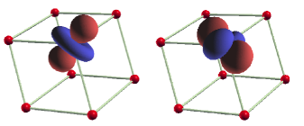
Figure 2: (Color online) $e_{\mathrm{g}}$-like ($3d_{3z^{2}-r^{2}}$ and $3d_{x^{2}-y^{2}}$) maximally localized Wannier functions for bcc Fe. The different tints denote regions with opposite sign.

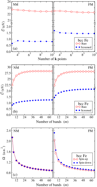
Figure 3: (Color online) Convergence of the average on-site matrix elements of the bare and screened Coulomb interaction between the 3d orbitals as a function of (a) the number of $\mathbf{k}$ points and (b) the number of bands used in the construction of the MLWF basis for the NM and FM states of bcc Fe. (c) The same as (b) for the average spread of the 3d orbitals.

In Fig. 3(a) we present a convergence study for the average on-site diagonal matrix elements of the bare and the screened Coulomb interaction ($\tilde{U}$) between the 3d orbitals as a function of the number of $\mathbf{k}$ points for the NM and the FM states of bcc Fe. Fig. 3(b) shows the same matrix elements as a function of the number of bands used in the construction of the MLWFs. We observe a fast $\mathbf{k}$-point convergence but a relatively slow convergence with respect to the number of bands. In fact, the screened $\tilde{U}$ is not completely converged even with 60 bands. The large difference between the NM and FM states will be discussed below.

The increase of the matrix elements of the Coulomb potential with the number of bands can be explained by the localization of the Wannier functions. In Fig. 3(c) we show the spread $\Omega$ for the 3d orbitals as a function of the number of bands. It can clearly be seen that $\Omega$ decreases if the number of bands increases, indicating that the 3d orbitals become more localized, which in turn gives rise to a larger $\tilde{U}$. For the rest of the 3d transition-metal series the behavior of the Coulomb matrix elements with respect to the number of bands is very similar to bcc Fe. In the rest of this section we use 6 bands and an $8\times 8\times 8$ $\mathbf{k}$-point mesh in order to compare our results with previously published data that adopted the same parameter settings.

In Table 1 we present the on-site matrix elements of the screened Coulomb potential for the NM and FM states of bcc Fe. Tables 2 and 3 contain the values for the FM state of fcc Co and Ni. For all three systems the average values for the diagonal ($\tilde{U}$) and off-diagonal ($\tilde{U}^{\prime}$, $\tilde{J}$) matrix elements are given in Table 4. We note that the splitting of the diagonal matrix elements by the crystal-field effect is quite pronounced. For bcc Fe the $e_{\mathrm{g}}$-like diagonal elements are larger than the $t_{2\mathrm{g}}$-like ones in the FM state, while in the NM state it is just the opposite. This means that the strongest interaction takes place between the electrons in the $e_{\mathrm{g}}$-like ($t_{2\mathrm{g}}$-like) orbitals for the FM (NM) state, because these are more localized. In the case of fcc Ni the situation is very similar. However, in fcc Co the splitting of the diagonal Coulomb matrix elements by the crystal-field effect is different: In the NM state (results not shown) all diagonal elements assume similar values, while in the FM state (see Table 2) the $t_{2\mathrm{g}}$-like diagonal elements are larger than the $e_{\mathrm{g}}$-like ones.

Table 1: Screened on-site direct ($\tilde{U}_{mn}=W_{mm,nn}^{\alpha\beta}$) and exchange ($\tilde{J}_{mn}=W_{mn,nm}^{\alpha\beta}$) Coulomb matrix elements between the 3d orbitals for FM bcc Fe within LSDA. In parentheses we show results for the NM state. We include 6 bands in the construction of the MLWFs. The indices 1 and 2 (3, 4, and 5) correspond to the $e_{\mathrm{g}}$-like ($t_{2\mathrm{g}}$-like) Wannier orbitals. All energies are in eV.

$\tilde{U}_{mn}$	1	2	3	4	5
1	1.63 (0.62)	0.35 (0.05)	0.64 (0.20)	0.64 (0.20)	0.31 (0.07)
2	0.35 (0.05)	1.63 (0.62)	0.42 (0.12)	0.42 (0.12)	0.75 (0.25)
3	0.64 (0.20)	0.42 (0.12)	1.33 (0.96)	0.38 (0.17)	0.38 (0.17)
4	0.64 (0.20)	0.42 (0.12)	0.38 (0.17)	1.33 (0.96)	0.38 (0.17)
5	0.31 (0.07)	0.75 (0.25)	0.38 (0.17)	0.38 (0.17)	1.33 (0.96)
$\tilde{J}_{mn}$	1	2	3	4	5
1	—	0.64 (0.28)	0.41 (0.30)	0.41 (0.30)	0.56 (0.37)
4	0.64 (0.28)	—	0.51 (0.35)	0.51 (0.35	0.35 (0.27)
3	0.41 (0.30)	0.51 (0.35)	—	0.47 (0.41)	0.47 (0.41)
2	0.41 (0.30)	0.51 (0.35)	0.47 (0.41)	—	0.47 (0.41)
5	0.56 (0.37)	0.35 (0.27)	0.47 (0.41)	0.47 (0.41)	—

Table 2: The same as Table 1 for the screened Coulomb potential for the FM state of fcc Co.

$\tilde{U}_{mn}$	1	2	3	4	5
1	1.20	0.22	0.54	0.51	0.24
2	0.22	1.20	0.36	0.32	0.59
3	0.54	0.36	1.45	0.38	0.39
4	0.51	0.32	0.38	1.45	0.36
5	0.24	0.59	0.39	0.36	1.45
$\tilde{J}_{mn}$	1	2	3	4	5
1	—	0.50	0.42	0.41	0.56
2	0.50	—	0.53	0.50	0.36
3	0.42	0.53	—	0.54	0.53
4	0.41	0.50	0.54	—	0.55
5	0.56	0.36	0.53	0.55	—

Table 3: The same as Table 2 for fcc Ni.

$\tilde{U}_{mn}$	1	2	3	4	5
1	1.53	0.28	0.57	0.58	0.26
2	0.28	1.53	0.35	0.37	0.66
3	0.57	0.35	1.33	0.34	0.33
4	0.58	0.37	0.34	1.33	0.33
5	0.26	0.66	0.33	0.33	1.33
$\tilde{J}_{mn}$	1	2	3	4	5
1	—	0.63	0.43	0.43	0.58
2	0.63	—	0.52	0.53	0.37
3	0.43	0.52	—	0.49	0.49
4	0.43	0.53	0.49	—	0.49
5	0.58	0.37	0.49	0.49	—

Table 4: Average screened on-site direct (diagonal $\tilde{U}$ and off-diagonal $\tilde{U}^{\prime}$) and exchange ($\tilde{J}$) Coulomb matrix elements between the 3d orbitals for FM 3d transition metals within LSDA. In parentheses we show results for the NM states. For comparison the LSDA+$U$ results ($U=1.9$ eV, $J=1.2$ eV) for fcc Ni are presented. We include 6 bands in the construction of the MLWFs. All energies are in eV.

	$\tilde{U}$	$\tilde{U}^{\prime}$	$\tilde{J}$
bcc Fe	1.45 (0.82)	0.47 (0.15)	0.48 (0.34)
fcc Co	1.35 (1.04)	0.39 (0.23)	0.49 (0.40)
fcc Ni	1.41 (1.28)	0.41 (0.34)	0.50 (0.46)
fcc Ni∗	1.49	0.44	0.51

^∗ LSDA+$U$

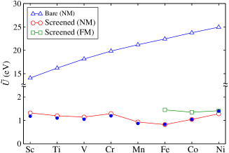
Figure 4: (Color online) Average bare and screened on-site direct ($\tilde{U}$) Coulomb matrix elements between the 3d orbitals for the series of 3d transition metals. For comparison results from Ref. Miyake, (filled spheres) are given. We include 6 bands in the construction of the MLWFs.

Figure 4 shows the average bare and screened on-site direct ($\tilde{U}$) Coulomb matrix elements for the series of 3d transition metals in the NM state. Results for the FM state of Fe, Co, and Ni are also included. Note that among all considered systems only the first three elements are not magnetic, while Cr and Mn order antiferromagnetically and Fe, Co, and Ni are ferromagnetic. The bare $\tilde{U}$ for the NM state increases linearly from 14 eV for Sc to 25 eV for Ni. This stems from the fact that, as one moves from the left to the right within one row of the periodic table, the nuclear charge increases and causes the 3d wave functions to contract. Hence the localization of the 3d electrons increases, giving rise to the observed trend for $\tilde{U}$. However, this trend is not observed for the screened Coulomb interaction, where the calculated values lie between 0.8 eV and 1.5 eV. As already seen in Table 1, the matrix elements of the screened Coulomb potential depend on the magnetic state. Figure 4 indicates that the $\tilde{U}$ values for the NM and FM states of Fe, Co, and Ni are also rather different, and this difference increases with the exchange splitting in the Ni-Co-Fe sequence. This observation can be qualitatively explained by the density of states (DOS) around the Fermi level presented in Fig. 5. As the screened Coulomb interaction depends on the polarizability, the number of occupied and unoccupied states around the Fermi level plays an important role in determining its strength. Bcc Fe in the NM state has the largest DOS around the Fermi energy and hence the smallest Coulomb matrix elements. However, for FM Fe the majority and minority-spin peaks at the Fermi level are shifted to lower and higher energies, respectively, due to the exchange field, leading to a lower DOS at the Fermi level. As a consequence, we obtain larger matrix elements. For the last three elements the calculated $\tilde{U}$, $\tilde{U}^{\prime}$, and $\tilde{J}$ values increase linearly for the NM state (see Table 4), while they are almost constant for the FM state. A comparison of our results for the screened Coulomb interaction in the NM state with Ref. Miyake, is given in Fig. 4. The agreement for the $\tilde{U}$ values is very good, and we find an equally good agreement for the $\tilde{J}$ values, which are not displayed in the figure.

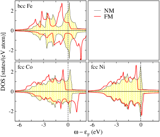
Figure 5: (Color online) Spin-resolved density of states for bcc Fe, fcc Co, and fcc Ni for the NM and FM states. The vertical dashed lines denote the Fermi level. Note that positive values of DOS refer to the majority-spin electrons and negative values to the minority-spin electrons.

To investigate the effect of static correlation on the matrix elements of the screened Coulomb interaction we present LSDA+$U$ results for $\tilde{U}$, $\tilde{U}^{\prime}$, and $\tilde{J}$ for the FM state of Ni in Table 4. The average matrix elements slightly increase relative to the LSDA. Again this observation can be explained by the scenario given above. Within the LSDA+$U$ scheme the exchange splitting of the Ni 3d states increases. This in turn gives rise to a larger magnetic moment (see Table 5) and a reduced DOS around the Fermi level. As a consequence, the Coulomb matrix elements increase. We expect a similar behavior for bcc Fe and fcc Co if the LSDA+$U$ scheme is employed.

Finally, we discuss the values of the matrix elements of the screened Coulomb potential $W$ used in the calculation of $R$ to make a connection with next section. The magnetic response function can be schematically written as

$$R=\frac{K}{1-WK}\>,$$ (33)

where the screened Coulomb potential $W$ in the denominator is responsible for the formation of collective spin-wave excitations. As shown above, the matrix elements of $W$ depend on the number of bands included in the construction of the MLWFs. The matrix elements of $K$ are considerably less sensitive to the number of bands; usually 10 bands are sufficient for 3d ferromagnets. For this reason, in the calculation of $R$ one might choose a particular $W$ that satisfies the exact condition $\lim_{\mathbf{q}\rightarrow\mathbf{0}}\omega(\mathbf{q})=0$ (Goldstone mode). For instance, in fcc Ni within LSDA one should include about 100 bands in order to fulfill the Goldstone theorem. Alternatively, one can calculate $W$ for a given number of bands and then scale it by a factor $\eta$, i.e., $W\rightarrow\eta W$, to obtain the Goldstone mode correctly. This second approach is computationally less demanding and is used in the present work. For 3d ferromagnets we calculate $W$ by including only 6 bands. In the case of fcc Ni the scaling factor is $\eta\approx 1.5$ within LSDA and $\eta\approx 1.8$ within LSDA+$U$. This means that the Coulomb matrix elements presented in Table 3 should be multiplied by 1.5 in the calculation of the magnetic response function $R$ within LSDA for fcc Ni. The violation of the Goldstone theorem within the present formalism stems from the approximations made in the calculation of the kernel $K$ and the screened Coulomb potential $W$. In a fully self-consistent linear-response calculation without additional approximations the Goldstone theorem should be fulfilled. However, this is hardly feasible in practice. When we manually reduce the exchange splitting of Ni by one-half within LSDA to simulate the renormalized Green function, the scaling factor is reduced to $\eta\approx 1.1$. Note that the LSDA overestimates the exchange splitting of Ni by a factor of 2 compared to experiments.exc_1 ; exc_2 In systems like bcc Fe for which the LSDA already provides a reasonable description of the electronic band structure compared to the experimentsexc_2 ; Singh ; Schindlmayr the scaling factor $\eta$ is close to 1.

IV Magnetic excitations in fcc Ni

This section deals with magnetic excitations in fcc Ni. Among the 3d ferromagnets Ni is known for particularly large discrepancies between the results from DFT calculations and experiments: The width of the occupied 3d bands in the LSDA is about 30% larger than that found in photoemission experiments, whereas the sp band width agrees within 10%.band_width ; band_width_2 Similarly, the LSDA yields a much smaller DOS [1.9 states/(eV atom)] at the Fermi level compared to low-temperature specific-heat data [3.0 states/(eV atom)], indicating a quasiparticle mass enhancement.dos_fermi Even larger discrepancies are obtained for the exchange splitting. Photoemission experiments give a small and highly anisotropic exchange splitting, 0.3 eV at the $\textrm{L}_{3}$ point and 0.2 eV at the $\textrm{X}_{2}$ point.exc_1 ; exc_2 In contrast, the LSDA yields a rather large (0.6 eV) and almost isotropic splitting.band_width However, the calculated magnetic moment turns out to be in good agreement with the experimental value.Ni_moment

Our calculated magnetic moments and exchange splittings within the LSDA and LSDA+$U$ are presented in Table 5. The corresponding band structures are given in Fig. 6. Within the LSDA the band structure, exchange splitting, and magnetic moment are in good accordance with literature values.band_width ; band_width_2 ; Ni_moment The inclusion of explicit static correlation in the form of a Hubbard $U$ within LSDA+$U$ slightly changes the electronic structure of Ni. In this case the exchange splitting is more anisotropic compared to the LSDA, i.e., it increases at the $\mathrm{L}_{3}$ point and decreases at the $\mathrm{X}_{2}$ point (see Table 5). The average exchange splitting increases within the LSDA+$U$ scheme however, and depending on the values of the Hubbard parameters $U$ and $J$ the LSDA+$U$ hence gives rise to a larger magnetic moment.

Table 5: Calculated magnetic moment $m$, exchange splitting at $\textrm{X}_{2}$ and $\textrm{L}_{3}$ as well as spin-wave stiffness constant $D$ in fcc Ni within LSDA and LSDA+$U$ with $U=1.9$ eV and $J=1.2$ eV. For comparison experimental values are given.

	$m$($\mu_{\mathrm{B}}$)	$\textrm{X}_{2}$(eV)	$\textrm{L}_{3}$(eV)	$D(\textrm{meV}\mathrm{{\AA}}^{2}$)
LSDA	0.61	0.61	0.57	740
LSDA+$U$	0.65	0.55	0.62	540
Expt.	0.60a	0.20b	0.30c	550d

^aRef. [Ni_moment, ]

^bRef. [exc_1, ]

^cRef. [exc_2, ]

^dRef. [Mook_2, ]

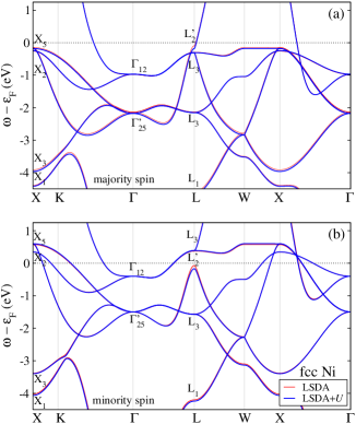
Figure 6: (Color online) LSDA and LSDA+$U$ ($U=1.9$ eV and $J=1.2$ eV) band structures of FM fcc Ni for (a) majority and (b) minority spins.

The magnetic response function $R$ [see Eq. (33)] contains all relevant information about the dynamics of the spin system. The poles of $K$ in the numerator correspond to the energies of single-particle spin-flip Stoner excitations, while the zeros of the denominator $(1-WK)$ describe collective spin-wave excitations. In the preceding section we showed that the convergence of the matrix elements of the screened Coulomb potential $W$ with respect to the number of $\mathbf{k}$ points (number of bands) is fast (slow), whereas the situation is opposite for the kernel $K$. For $W$ we take the values from Sec. III, scaled by an appropriate factor $\eta$, while we construct $K$ using 5 MLWFs, 15 occupied and unoccupied bands per spin channel, and a very dense $40\times 40\times 40$ $\mathbf{k}$-point sampling. The Brillouin-zone summations in $K$ are performed with the tetrahedron method.Tetrahedron The calculation of $R$ is carried out for a fixed $\mathbf{q}$ as a function of energy $\omega$ up to 1.5 eV.

The remainder of this section is divided into two parts. In the first part the single-particle Stoner excitations are presented. The second part deals with the collective spin-wave excitations.

IV.1 Single-particle Stoner excitations

Stoner excitations are electron transitions between bands of opposite spin. When an electron is excited from an occupied majority-spin state at $\mathbf{k}$ to an unoccupied minority-spin state at $\mathbf{k}$+$\mathbf{q}$, it produces an electron-hole pair with triplet spin configuration that reduces the magnetization by unity. Therefore, these excitations are associated with longitudinal fluctuations of the magnetization and play an important role in determining the high-temperature properties of magnetic materials.Moriya To simplify the discussion, let us consider a free electron gas with parabolic dispersion and a rigid exchange splitting $\Delta E_{\textrm{ex}}$. The corresponding single-particle excitation energies are given by $\omega(\mathbf{q})=(\pm 2\mathbf{k}\cdot\mathbf{q}+\mathbf{q}^{2})+\Delta E_{\textrm{ex}}$. For $\mathbf{q}\rightarrow\mathbf{0}$ the necessary energy for such excitations equals the exchange splitting $\Delta E_{\textrm{ex}}$, but for finite $\mathbf{q}$ these excitations form a continuous spectrum, which is called the Stoner continuum and is determined by all possible values of $\mathbf{k}$. The upper and lower bounds of the Stoner continuum depend on the electronic band structure of the material. For example, in strong ferromagnets the smallest possible excitation energy is given by the Stoner gap $\Delta S$. On the other hand, weak ferromagnets exhibit a vanishing gap $\Delta S=0$, and thus single-particle excitations do not require a finite energy for particular $\mathbf{q}$ values. The lower bound is of special interest, because when the collective spin-wave excitations enter the Stoner continuum, they start to decay into single-particle excitations, which reduces their lifetime drastically. We note that the picture of Stoner excitations in real materials is different from the free electron gas with a single band.Kuzemsky

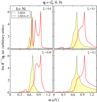
Figure 7: (Color online) The Kohn-Sham magnetic response function for fcc Ni for selected wave vectors along the $\Gamma-\textrm{X}$ direction in the Brillouin zone. Since the Kohn-Sham system is noninteracting, the spectrum exhibits only single-particle Stoner excitations but no collective magnon modes at lower energies. In each panel the peak amplitudes are scaled to the same height.

Since the Stoner excitations are single-particle spin-flip processes, they can be studied qualitatively at the Kohn-Sham level. They result from the term $\textrm{Im}\,K$, as discussed before. In Fig. 7 we present the imaginary part of the Kohn-Sham magnetic response function for fcc Ni for selected wave vectors along the $\Gamma-\textrm{X}$ direction. Note that all peak amplitudes are scaled to the same height. The energetic position and shape of the Stoner spectrum for $\mathbf{q}=\mathbf{0}$ provide a measure for the mean exchange splitting and its variation across the Brillouin zone. The triple-peak structure reflects the intraband and interband transitions. The position of the first peak gives the mean exchange splitting: 0.61 eV within LSDA and 0.69 eV within LSDA+$U$. The broadening of the peaks reflects the $\mathbf{k}$-dependence of the exchange splitting. For rigidly split bands one would get $\delta$ peaks. As the wave vector increases, individual peaks become broader and are no longer distinguishable. Since the Kohn-Sham system is noninteracting, the spectrum does not exhibit collective magnon modes at low energies.

Experimentally, Stoner excitations in 3d ferromagnets are studied with spin-polarized electron-energy-loss spectroscopy (SPEELS), a technique that not only measures the high-energy Stoner excitations but also low-energy collective spin-wave modes up to the Brillouin-zone boundary. Using SPEELS Kirschner et al.Kirschner_1 studied the Stoner excitation spectrum of Ni at $\mathbf{q}\approx\mathbf{0}$. The authors found that the spectrum had a broad energy distribution of 0.3 eV (full width at half maximum) and was centered around 0.3 eV, which is consistent with the average exchange splitting determined by photoemission experiments. Additionally, the width of the distribution provided evidence for the pronounced $\mathbf{k}$-dependence of the exchange splitting. The comparison of our calculated spectra with the experimental data shows large discrepancies, however. These can be attributed to the overestimated exchange splitting and its incorrect nearly isotropic behavior over the Brillouin zone in the LSDA. As pointed out by Oles and StollhoffOles and by Liebsch,Liebsch the large exchange splitting in the LSDA is due to the neglect of strong correlation effects within the 3d states and anisotropic exchange. Consequently, recent studies by Katsnelson and LichtensteinDMFT_1 and by Grechnev et al.DMFT_2 based on dynamical mean-field theory, in which the exchange and correlation effects are taken into account properly, gave much improved results for the exchange splitting and quasiparticle band structure of Ni.

IV.2 Collective spin-wave excitations

In the preceding section we discussed the non-interacting magnetic response function $K$, which has singularities that correspond to single-particle Stoner excitations, usually with a broad energy distribution. In addition, there may be other singularities of $R$ for a fixed $\mathbf{q}$. For some $\omega(\mathbf{q})$ outside the Stoner continuum the denominator ($1-WK$) of the magnetic response function might vanish, indicating collective spin-wave excitations. These correspond to transverse fluctuations of the direction of the magnetization and can be interpreted as a coherent superposition of an electron and a hole with opposite spins coupled via an attractive screened Coulomb interaction $W$, thereby forming a bound state with energy $\omega(\mathbf{q})$, spin $1$, and momentum $\mathbf{q}$.Pines As more than one particle is involved in the excitation process, the formation of spin waves cannot be described within a single-particle picture.

Before discussing our numerical results we briefly review the status of experimental and theoretical studies of magnetic excitations in fcc Ni. Starting from the mid 1960s the spin dynamics of ferromagnetic 3d transition metals and their alloys were intensively investigated by inelastic neutron scattering. The first experiments for Ni were performed at high temperatures and in the low-energy region. Later the measurements were extended to higher energies. The results of these early neutron-scattering experiments and a comparison with realistic band structure calculations can be found in the review article by Lowde and Windsor.Windsor However, the signal intensity and energy resolution in these early experiments were not favorable for a quantitative determination of the spin-wave excitations in Ni. More precise measurements were reported by Mook and collaborators in the 1980s with emphasis on high energies up to 240 meV.Mook_1 ; Mook_2 ; Mook_3 The authors measured the spin-wave dispersion of Ni at several temperatures starting from $T=4.2\,\textrm{K}$ up to $T\approx 2T_{\mathrm{C}}$, where $T_{\mathrm{C}}=631\,\textrm{K}$ is the Curie temperature, and found that the spin-wave dispersion was isotropic in $\mathbf{q}$ over the entire temperature range studied. The obtained spin-wave stiffness constant was $D=550$ meV $\mathrm{{\AA}}^{2}$ at $T=4.2\,\textrm{K}$ and $D=505$ meV $\mathrm{{\AA}}^{2}$ at $T=295\,\textrm{K}$. The spin-wave intensity was found to decrease faster with increasing energy in the $[1\,1\,1]$ direction than along other symmetry directions. In all directions the spin waves eventually disappeared at some wave vector close to the zone boundary inside the first Brillouin zone, which was attributed to a decay into Stoner excitations. Additionally, the authors found evidence for a second branch in the spin-wave dispersion, i.e., an optical mode that crosses the main $[1\,0\,0]$ acoustic branch around 125 meV. However, inelastic neutron scattering does not allow to explore the entire Brillouin zone in 3d ferromagnets, in contrast to SPEELS. Using SPEELS Abraham and HopsterAbraham attempted to study short-wave-length (or large-wave-vector) spin excitations in Ni. However, they only detected Stoner excitations, although the data reported reaches down to 100 meV and the resolution of the instrument (17 meV) should have been sufficient to observe collective excitations. A qualitative explanation for the absence of spin-wave peaks in the SPEELS spectrum was given by Hong and Mills,Hong who showed that the spin waves can only be observed in SPEELS if the exchange splitting of the 3d bands is large compared to the spin-wave excitation energies. Indeed, spin waves up to the Brillouin-zone boundary are observed in Fe and Co, which have substantially larger exchange splittings than Ni.Speels_1 ; Speels_2 ; Speels_3 ; Speels_4

On the theoretical side, the first attempt to use realistic energy bands for Ni in the calculations of a generalized susceptibility was undertaken by Lowde and Windsor.Windsor The authors calculated the magnetic susceptibility within the RPA for rigidly spin-split bands, but the agreement with the available experimental data was not good. Cooke et al.Cooke_1 ; Cooke_2 ; Cooke_3 showed that it is necessary to take the $\mathbf{k}$-dependence of the exchange splitting into account for a quantitative comparison between theory and experiment. They used a tight-binding description of the electronic energy bands, and the ferromagnetism was driven by an empirical on-site Coulomb interaction between the 3d electrons with two adjustable parameters. These parameters were chosen in such a way that the calculations reproduce the experimentally observed magnetic moment as well as the correct $t_{2\mathrm{g}}$ and $e_{\mathrm{g}}$ character of the moment as measured in neutron magnetic-form-factor experiments. The calculations of Cooke et al. not only yielded the correct spin-wave dispersion relation, including the appearance of the optical branch in the $[1\,0\,0]$ direction, but the damping of the spin waves in the presence of the Stoner modes was also correctly described. A similar approach was used by Hong and MillsHong with an empirical Coulomb interaction that was form-invariant under spin rotations. However, they failed to find the optical mode in the spin-wave dispersion of Ni.

A much more accurate description of spin waves in ferromagnetic 3d transition metals was reported by SavrasovSavrasov_SW and by Karlsson and Aryasetiawan.Karlsson_1 In both works spin-polarized DFT was used for the ground-state calculations. For the transverse spin susceptibility Savrasov employed TDDFT, while Karlsson and Aryasetiawan adopted MBPT. Similar to the findings of Cooke et al., Savrasov obtained two branches in the spin-wave dispersion of Ni along the $[1\,0\,0]$ direction with an optical mode at high energies. Karlsson and Aryasetiawan confirmed these results and investigated the role of the one-particle band structure on the spin-wave dispersion. They found a very good agreement between theory and experiment if the LSDA exchange splitting was manually reduced by one-half. Additionally, the calculations gave evidence for an optical branch along the $[1\,1\,1]$ direction.

The optical branch in the spin-wave dispersion of Ni is evidently a very subtle issue. So far, there has been no general consensus in theoretical treatments concerning the sensitivity of the results to the details of the electronic structure and to the method used. In the following we hence focus on the energy region where the double-peak structure is observed in the spin-wave spectrum. To illuminate the effect of the electronic structure on the magnetic excitation spectrum of Ni we employ three different methods: LSDA, LSDA+$U$, and LSDA with a reduced exchange splitting by one-half. The calculated spin-wave dispersion along the high-symmetry lines $\textrm{L}-\Gamma-\textrm{X}$ is displayed in Fig. 8. For comparison the experimental dispersion is also shown. The LSDA and LSDA+$U$ yield qualitatively similar results, with an optical mode not only in the $[1\,0\,0]$ but also in the $[1\,1\,1]$ direction. The acoustic branch is well described within LSDA and LSDA+$U$, but the optical branch is too high in energy. This discrepancy between theory and experiment can be traced back to the overestimation of the exchange splitting in the LSDA.Karlsson_1 Indeed, when we reduce the exchange splitting by one-half as in Ref. Karlsson_1, , we obtain reasonable agreement with the experiments. The corresponding dispersion, shown in Fig. 8(c), is similar to that of Karlsson and Aryasetiawan.Karlsson_1

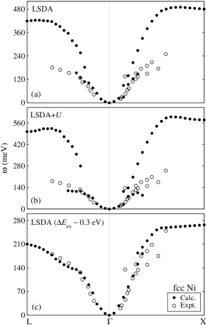
Figure 8: Spin-wave dispersion for fcc Ni along high-symmetry lines $(\textrm{L}-\Gamma-\textrm{X})$ in the Brillouin zone within (a) LSDA, (b) LSDA+$U$, and (c) LSDA with a reduced exchange splitting. The experimental dispersion is taken from Refs. Mook_2, and Mook_3, .

In Fig. 9 we show the imaginary part of the magnetic response function $R$ for selected wave vectors along the $[1\,0\,0]$ and $[1\,1\,1]$ directions. The peak amplitudes are again scaled to the same height for presentational purposes. The obtained spin-wave spectra along $[1\,0\,0]$ are in very good agreement with previous calculations.Savrasov_SW ; Karlsson_1 In particular, a double-peak structure starts to develop from $\mathbf{q}=(0.15,\,0,\,0)$. For larger wave vectors the two peaks overlap, resulting in a rather broad single feature, which can be decomposed into two Lorentzian peaks as shown in Fig. 10 for $\mathbf{q}=(0.25,\,0,\,0)$. As the wave vector increases, the intensity of the lower peak decreases in agreement with experiments.Mook_3 In the $[1\,1\,1]$ direction the double peak is not so clear within the LSDA. Nevertheless, the calculated structure can still be decomposed into two Lorentzians (results not shown), but the $\mathbf{q}$ interval where the double-peak structure appears is small compared to the $[1\,0\,0]$ direction.

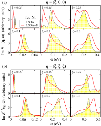
Figure 9: (Color online) Spin-wave excitation spectra for fcc Ni within LSDA and LSDA+$U$ for selected wave vectors along (a) the $[1\,0\,0]$ and (b) the $[1\,1\,1]$ directions in the Brillouin zone. The double-peak structure for certain wave vectors is clearly visible. All peak amplitudes are scaled to the same height.

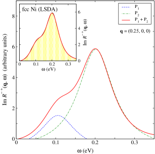
Figure 10: (Color online) Decomposition of the single feature for $\mathbf{q}=(0.25,0,0)$ into two Lorentzian peaks. In the inset we compare with the original curve.

Our calculations show that the exchange splitting has a strong influence on the emergence of a double-peak structure. To demonstrate this we consider two $\mathbf{q}$ points in the $[1\,0\,0]$ direction where such features appear and calculate the LSDA spin-wave spectra by reducing the exchange splitting gradually by 0.1 eV in each step, up to one-half of its original value. The results are presented in Fig. 11. Even a very small reduction in the exchange splitting by 0.1 eV strongly suppresses the double-peak feature. As the exchange splitting reduces further, the width of the peaks becomes narrower, indicating an increased spin-wave life time. When the exchange splitting is reduced by one-half and corresponds to the experimental value, the optical branch completely disappears in the $[1\,1\,1]$ direction, while it is shifted to larger wave vectors in the $[1\,0\,0]$ direction. The situation is very similar within LSDA+$U$ with a reduced exchange splitting. Karlsson and Aryasetiawan found a weak double-peak structure with a reduced exchange splitting for $\mathbf{q}=0.1875(1,\,1,\,1)$ when they used a small Gaussian broadening parameter in the Brillouin-zone integration,Karlsson_1 but this double-peak structure becomes smeared out if a larger broadening is used. Based on the symmetry properties of fcc Ni, the spin-wave dispersion should be isotropic, i.e., one expects an optical branch also in the $[1\,1\,1]$ direction, but the resolution of the presently available experimental data is not sufficient to observe it.Mook_3 Of course, a reduction of the exchange splitting in the calculations does not solve all problems for Ni. In particular, too large band widths and the incorrect isotropic exchange splitting remain important issues whose effect on the spin-wave spectra requires further investigations.

As pointed out by Cooke et al.,Cooke_2 the double-peak structure in the magnetic excitation spectra of 3d ferromagnets stems from the $\mathbf{k}$-dependent exchange splitting and interband transitions. A detailed analysis was given by Karlsson and Aryasetiawan,Karlsson_1 who showed that the double-peak structure in fcc Ni is implicitly contained in the kernel $K$, i.e., it is a band-structure effect arising from the fact that $W\textrm{Im}\,K$ possesses additional structure below the Stoner peak, which in turn gives rise to a weak dip structure in $(1-W\textrm{Re}\,K)$ via the Hilbert transformation. Such a weak dip structure appears as a second peak in the spin-wave excitation spectrum for particular wave vectors. This observation is indirectly confirmed by our analysis. The application of a Hubbard $U$ in the LSDA+$U$ calculation shifts majority-spin and minority-spin states more or less rigidly, and the optical branch appears in the LSDA and LSDA+$U$ around the same wave vector $\mathbf{q}$ along $[1\,0\,0]$, while a reduction of the exchange splitting leads to an appearance of the optical branch at higher $\mathbf{q}$ values.

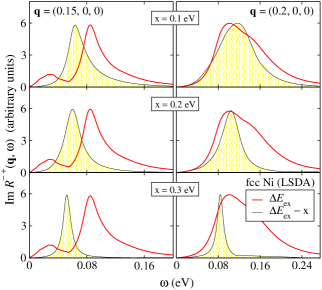
Figure 11: (Color online) Same as Fig. 9 for $\mathbf{q}=(0.15,0,0)$ and $\mathbf{q}=(0.2,0,0)$ for different exchange splitting within LSDA. The spectra for the original LSDA exchange splitting are included for comparison.

The magnetic response function $R$ allows to extract information about the spin-wave life times, which are inversely proportional to the widths of the spin-wave peaks. If Ni were a strong ferromagnet, one would get well defined $\delta$ peaks up to about 0.3 eV in the spin-wave spectra, corresponding to the energy difference between the highest occupied majority-spin 3d band and the Fermi level, i.e., the Stoner gap. However, Ni is not a truly strong ferromagnet due to the sp-d hybridized majority states around the Fermi energy, and Stoner excitations thus occur essentially at all energies. This means that spin waves decay into Stoner excitations for all non-zero wave vectors, which is reflected by a finite width of the spin-wave peaks as shown in Fig. 9. The life time of the spin waves depends on the details of the coupling between these excitations and on the density of states of the Stoner excitations. It should be noted that in itinerant ferromagnets the life time of the spin waves becomes infinite in the limit of a vanishing wave vector, provided that spin-orbit coupling is ignored. As seen in Fig. 9, for small wave vectors the spin-wave peaks are indeed narrow, and the damping is hence weak, i.e., the life times are long. As the wave vector increases, the spin-wave dispersion enters into the region with a high density of states of Stoner excitations, and the decay mechanism becomes more efficient. In both crystallographic directions considered here the maximum damping occurs in the region where the double-peak structure appears. In contrast to the findings of Cooke et al.,Cooke_2 the spin-wave peaks associated with the optical branch are narrower than the acoustic ones in our work, and the peak widths stay almost constant throughout the Brillouin zone, while the peak widths in the acoustic branch increase with the wave vector. This might in fact explain why the acoustic branch disappears in the middle of the Brillouin zone in the neutron-scattering experiments.Mook_3

Finally, we focus on the spin-wave stiffness constant $D$. In ferromagnets the spin waves show a quadratic dispersion law $\omega(\mathbf{q})=Dq^{2}$ for small wave vectors. The values for Ni obtained with different methods are listed in Table 5. Our LSDA estimate of $740\,\textrm{meV}\,\mathrm{{\AA}}^{2}$ is substantially larger than the experimental value $550\,\textrm{meV}\,\mathrm{{\AA}}^{2}$. With the reduced exchange splitting $D$ increases even further to $870\,\textrm{meV}\,\mathrm{{\AA}}^{2}$, whereas LSDA+$U$ provides a much better estimate of $540\,\textrm{meV}\,\mathrm{{\AA}}^{2}$, which reflects the importance of static correlation effects in Ni. We note that our LSDA estimate for the spin-wave stiffness of fcc Ni is in good agreement with calculations based on constrained DFT in the adiabatic approximation. Using the frozen-magnon technique Rosengaard and JohanssonJohansson found $D=739\,\textrm{meV}\,\textrm{{\AA}}^{2}$, which is very similar to the values obtained by Schilfgaarde and AntropovSchilfgaarde ($740\,\textrm{meV}\,\textrm{{\AA}}^{2}$) and by Pajda et al.Pajda ($756\pm 29\,\textrm{meV}\,\textrm{{\AA}}^{2}$), who employed real-space methods. As the adiabatic approximation becomes exact in the limit of long wave lengths ($\mathbf{q}\rightarrow\mathbf{0}$),Katsnelson_1 this can be compared with values obtained from more rigorous approaches based on the dynamical transverse spin susceptibility or magnetic response function. However, within constrained DFT the second branch in the spin-wave dispersion of Ni cannot be described.

V Conclusions and outlook

In conclusion, we have developed a computational method to study excitation spectra of magnetic materials from first principles. The method is based on many-body perturbation theory. The main quantity of interest is the transverse magnetic response function, which treats both collective spin-wave excitations and single-particle spin-flip Stoner excitations on an equal footing. In order to describe the former we include appropriate vertex corrections in the form of a multiple-scattering $T$-matrix, which describes the coupling of electrons and holes with different spins. To reduce the numerical cost for the calculation of the four-point $T$-matrix we exploit a transformation to maximally localized Wannier functions that takes advantage of the short spatial range of electronic correlation in the partially filled d or f orbitals of magnetic materials. Our implementation is based on the FLAPW method.

The developed scheme was employed to calculate the matrix elements of the Coulomb potential for the series of 3d transition metals in the MLWF basis. Special attention was given to the ferromagnets Fe, Co and Ni. We showed that the matrix elements of the screened Coulomb potential are rather different for the NM and FM states and that the difference increases with the exchange splitting in the Ni-Co-Fe sequence, which can be accounted for on the basis of the total density of states around the Fermi level for the corresponding systems.

The magnetic excitations in fcc Ni were studied in detail based on the LSDA and LSDA+$U$ methods. Both schemes give qualitatively similar results for the spin-wave spectra and dispersion. However, correlation effects seem to be important for the spin-wave stiffness constant, which is overestimated within LSDA. Our calculations indicate the existence of an optical branch in the spin-wave dispersion of Ni along the $[1\,1\,1]$ in addition to that along the $[1\,0\,0]$ direction in the Brillouin zone. Although the acoustic branch is well described within LSDA and LSDA+$U$, the optical branch appears to be too high in energy. This discrepancy between theory and experiment can be attributed to the overestimation of the exchange splitting or, in other words, to the use of the Kohn-Sham Green function in the calculation of the kernel $K$ instead of the renormalized one.

In the LSDA Kohn-Sham Green function the long and short-range correlation effects are not taken into account properly. The former can be treated within the $GW$ approximation, while the latter require the summation of spin-dependent $T$-matrix contributions. In the future we plan to incorporate electron-electron (hole-hole) and electron-magnon scattering processes into the electronic self-energy by means of the $T$-matrix formalism, which improves the theoretical description of the quasiparticle band structure. In particular, it is expected to yield the correct exchange splitting in magnetic materials.

- (1) T. Moriya, Spin Fluctuations in Itinerant Electron Magnetism (Springer, Berlin, 1985).
- (2) U. Köbler, A. Hoser, H.A. Graf, M.-T. Fernandez-Diaz, K. Fischer, and T. Brückel, Eur. Phys. J. B 8, 217 (1999).
- (3) N. D. Mermin and H. Wagner, Phys. Rev. Lett. 17, 1133 (1966); 17, 1307(E) (1966).
- (4) A. Hofmann, X. Y. Cui, J. Schäfer, S. Meyer P. Höpfner, C. Blumenstein, M. Paul, L. Patthey, E. Rotenberg, J. Bünemann, F. Gebhard, T. Ohm, W. Weber, and R. Claessen, Phys. Rev. Lett. 102, 187204 (2009).
- (5) J. Hong and D. L. Mills, Phys. Rev. B 59, 13840 (1999).
- (6) J. Hong and D. L. Mills, Phys. Rev. B 62, 5589 (2000).
- (7) V. P. Zhukov, E. V. Chulkov, and P. M. Echenique, Phys. Rev. Lett. 93, 096401 (2004); Phys. Rev. B 72, 155109 (2005); 73, 125105 (2006).
- (8) I. A. Nechaev, I. Yu. Sklyadneva, V. M. Silkin, P. M. Echenique, and E. V. Chulkov, Phys. Rev. B 78, 085113 (2008).
- (9) E. Dagotto, Rev. Mod. Phys. 66, 763 (1994).
- (10) D. J. Scalapino, Phys. Rep. 250, 329 (1995).
- (11) J. P. Carbotte, E. Schachinger, and D. N. Basov, Nature 401, 354 (1999).
- (12) T. Dahm, V. Hinkov, S. V. Borisenko, A. A. Kordyuk, V. B. Zabolotnyy, J. Fink, B. Büchner, D. J. Scalapino, W. Hanke, and B. Keimer, Nature Phys. 5, 217 (2009).
- (13) B. C. Choi, M. Belov, W. K. Hiebert, G. E. Ballentine, and M. R. Freeman, Phys. Rev. Lett. 86, 728 (2001).
- (14) M. Farle, Rep. Prog. Phys. 61, 755 (1998).
- (15) J. Kübler, Theory of Itinerant Electron Magnetism (Clarendon Press, Oxford, 2000).
- (16) L. M. Sandratskii, Adv. Phys. 47, 91 (1998).
- (17) L. Nordström and D. J. Singh, Phys. Rev. Lett. 76, 4420 (1996).
- (18) N. M. Rosengaard and B. Johansson, Phys. Rev. B 55, 14975 (1997).
- (19) S. V. Halilov, H. Eschrig, A. Y. Perlov, and P. M. Oppeneer, Phys. Rev. B 58, 293 (1998).
- (20) M. van Schilfgaarde and V. P. Antropov, J. Appl. Phys. 85, 4827 (1999).
- (21) O. Grotheer, C. Ederer, and M. Fähnle, Phys. Rev. B 63, 100401 (2001).
- (22) M. Pajda, J. Kudrnovský, I. Turek, V. Drchal, and P. Bruno, Phys. Rev. B 64, 174402 (2001).
- (23) J. F. Cooke, Phys. Rev. B 7, 1108 (1973).
- (24) J. F. Cooke, J. W. Lynn, and H. L. Davis, Phys. Rev. B 21, 4118 (1980).
- (25) J. F. Cooke, J. A. Blackman, and T. Morgan, Phys. Rev. Lett. 54, 718 (1985).
- (26) J. A. Blackman, T. Morgan, and J. F. Cooke, Phys. Rev. Lett. 55, 2814 (1985); K. N. Trohidou, J. A. Blackman, and J. F. Cooke, Phys. Rev. Lett. 67, 2561 (1991).
- (27) H. Tang, M. Plihal, and D. L. Mills, J. Magn. Magn. Mater. 157, 23 (1998).
- (28) R. B. Muniz and D. L. Mills, Phys. Rev. B 66, 174417 (2002).
- (29) A. T. Costa, R. B. Muniz, and D. L. Mills, J. Phys.: Condens. Matter 15, S495 (2003); Phys. Rev. B 68, 224435 (2003); 69, 064413 (2004); 70, 054406 (2004); 74, 214403 (2006).
- (30) A. T. Costa, R. B. Muniz, J. X. Cao, R. Q. Wu, and D. L. Mills, Phys. Rev. B 78, 054439 (2008).
- (31) S. Y. Savrasov, Phys. Rev. Lett. 81, 2570 (1998).
- (32) P. Buczek, A. Ernst, L. Sandratskii, and P. Bruno, J. Magn. Magn. Mater. (to be published); P. Buczek, A. Ernst, P. Bruno, and L. M. Sandratskii, Phys. Rev. Lett. 102, 247206 (2009).
- (33) K. Karlsson and F. Aryasetiawan, Phys. Rev. B 62, 3006 (2000); J. Phys.: Condens. Matter 12, 7617 (2000).
- (34) F. Aryasetiawan and K. Karlsson, Phys. Rev. B 60, 7419 (1999).
- (35) G. Strinati, La Rivista del Nuovo Cimento 11, 1 (1988).
- (36) N. Marzari and D. Vanderbilt, Phys. Rev. B 56, 12847 (1997).
- (37) I. Souza, N. Marzari, and D. Vanderbilt, Phys. Rev. B 65, 035109 (2001).
- (38) O. K. Andersen and T. Saha-Dasgupta, Phys. Rev. B 62, R16219 (2000); Bull. Mater. Sci. 26, 19 (2003).
- (39) G. Berghold, C. J. Mundy, A. H. Romero, J. Hutter, and M. Parrinello, Phys. Rev. B 61, 10040 (2000).
- (40) M. Posternak, A. Baldereschi, S. Massidda, and N. Marzari, Phys. Rev. B 65, 184422 (2002).
- (41) K. S. Thygesen, L. B. Hansen, and K. W. Jacobsen, Phys. Rev. Lett. 94, 026405 (2005); Phys. Rev. B 72, 125119 (2005).
- (42) H. Weng, T. Ozaki, and K. Terakura, Phys. Rev. B 79, 235118 (2009).
- (43) W. Ku, H. Rosner, W. E. Pickett, and R. T. Scalettar, Phys. Rev. Lett. 89, 167204 (2002).
- (44) E. Pavarini, S. Biermann, A. Poteryaev, A. I. Lichtenstein, A. Georges, and O. K. Andersen, Phys. Rev. Lett. 92, 176403 (2004).
- (45) F. Lechermann, A. Georges, A. Poteryaev, S. Biermann, M. Posternak, A. Yamasaki, and O. K. Andersen, Phys. Rev. B 74, 125120 (2006); M. Aichhorn, L. Pourovskii, V. Vildosola, M. Ferrero, O. Parcollet, T. Miyake, A. Georges, and S. Biermann, Phys. Rev. B 80, 085101 (2009).
- (46) V. I. Anisimov, D. E. Kondakov, A. V. Kozhevnikov, I. A. Nekrasov, Z. V. Pchelkina, J. W. Allen, S.-K. Mo, H.-D. Kim, P. Metcalf, S. Suga, A. Sekiyama, G. Keller, I. Leonov, X. Ren, and D. Vollhardt, Phys. Rev. B 71, 125119 (2005); M. M. Korshunov, V. A. Gavrichkov, S. G. Ovchinnikov, I. A. Nekrasov, Z. V. Pchelkina, and V. I. Anisimov, Phys. Rev. B 72, 165104 (2005).
- (47) L. Hedin, Phys. Rev. 139, A796 (1965).
- (48) F. Aryasetiawan and O. Gunnarsson, Phys. Rev. B 49, 16214 (1994).
- (49) T. Kotani and M. van Schilfgaarde, Solid State Commun. 121, 461 (2002).
- (50) C. Friedrich, A. Schindlmayr, and S. Blügel, Comput. Phys. Commun. 180, 347 (2009).
- (51) C. Friedrich, S. Blügel, and A. Schindlmayr, Phys. Rev. B. (to be published)
- (52) http://www.flapw.de
- (53) J. P. Perdew and A. Zunger, Phys. Rev. B 23, 5048 (1981).
- (54) P.H. Dederichs, S. Blügel, R. Zeller, and H. Akai, Phys. Rev. Lett. 53, 2512 (1984).
- (55) F. Aryasetiawan, M. Imada, A. Georges, G. Kotliar, S. Biermann, and A. I. Lichtenstein, Phys. Rev. B 70, 195104 (2004); F. Aryasetiawan, K. Karlsson, O. Jepsen, and U. Schönberger, Phys. Rev. B 74, 125106 (2006).
- (56) T. Miyake, F. Aryasetiawan, and M. Imada, Phys. Rev. B 80, 155134 (2009).
- (57) T. Miyake and F. Aryasetiawan, Phys. Rev. B 77, 085122 (2008).
- (58) I. Yang, S. Y. Savrasov, and G. Kotliar, Phys. Rev. Lett. 87, 216405 (2001).
- (59) A. A. Mostofi, J. R. Yates, Y.-S. Lee, I. Souza, D. Vanderbilt, and N. Marzari, Comput. Phys. Commun. 178, 685 (2008).
- (60) F. Freimuth, Y. Mokrousov, D. Wortmann, S. Heinze, and S. Blügel, Phys. Rev. B 78, 035120 (2008).
- (61) M. Springer and F. Aryasetiawan, Phys. Rev. B 57, 4364 (1998).
- (62) T. Kotani, J. Phys.: Condens. Matter 12, 2413 (2000).
- (63) I. Schnell, G. Czycholl, and R. C. Albers, Phys. Rev. B 65, 075103 (2002); 68, 245102 (2003).
- (64) M. Cococcioni and S. de Gironcoli, Phys. Rev. B 71, 035105 (2005).
- (65) I. V. Solovyev and M. Imada, Phys. Rev. B 71, 045103 (2005); I. V. Solovyev, Phys. Rev. Lett. 95, 267205 (2005).
- (66) K. Nakamura, R. Arita, Y. Yoshimoto, and S. Tsuneyuki, Phys. Rev. B 74, 235113 (2006).
- (67) W. Eberhardt and E. W. Plummer, Phys. Rev. B 21, 3245 (1980).
- (68) C. S. Wang and J. Callaway, Phys. Rev. B 15, 298 (1977).
- (69) M. Dixon, F. E. Hoare, T. M. Holden, and D. E. Moody, Proc. R. Soc. A 285, 561 (1965).
- (70) R. Raue and H. Hopster, Z. Phys. B 54, 121 (1984).
- (71) D. E. Eastman, F. J. Himpsel, and J. A. Knapp, Phys. Rev. Lett. 44, 95 (1980).
- (72) V. Iota, J.-H. P. Klepeis, C.-S. Yoo, J. Lang, D. Haskel, and G. Srajer, Appl. Phys. Lett. 90, 042505 (2007).
- (73) M. Singh, C. S. Wang, and J. Callaway, Phys. Rev. B 11, 287 (1975).
- (74) A. Schindlmayr, C. Friedrich, E. Şaşıoğlu, and S. Blügel, Z. Phys. Chem. (to be published).
- (75) J. Rath and A. J. Freeman, Phys. Rev. B 11, 2109 (1975).
- (76) A. L. Kuzemsky, Int. J. Mod. Phys. B 16, 803 (2002).
- (77) J. Kirschner, D. Rebenstorff, and H. Ibach, Phys. Rev. Lett. 53, 698 (1984).
- (78) A. M. Oles and G. Stollhoff, Phys. Rev. B 29, 314 (1984).
- (79) A. Liebsch, Phys. Rev. B 23, 5203 (1981).
- (80) M. I. Katsnelson and A. I. Lichtenstein, Eur. Phys. J. B 30, 9 (2002).
- (81) A. Grechnev, I. Di Marco, M. I. Katsnelson, A. I. Lichtenstein, J. Wills, and O. Eriksson, Phys. Rev. B 76, 035107 (2007).
- (82) D. Pines, The Many Body Problem (Benjamin, New York, 1962).
- (83) R. D. Lowde and C. G. Windsor, Adv. Phys. 19, 813 (1970).
- (84) H. A. Mook and D. Tocchetti, Phys. Rev. Lett. 43, 2029 (1979).
- (85) J. W. Lynn and H. A. Mook, Phys. Rev. B 23, 198 (1981).
- (86) H. A. Mook and D. McK. Paul, Phys. Rev. Lett. 54, 227 (1985).
- (87) D. L. Abraham and H. Hopster, Phys. Rev. Lett. 62, 1157 (1989).
- (88) M. Plihal, D. L. Mills, and J. Kirschner, Phys. Rev. Lett. 82, 2579 (1999).
- (89) R. Vollmer, M. Etzkorn, P. S. A. Kumar, H. Ibach, and J. Kirschner, Phys. Rev. Lett. 91, 147201 (2003).
- (90) W. X. Tang, Y. Zhang, I. Tudosa, J. Prokop, M. Etzkorn, and J. Kirschner, Phys. Rev. Lett. 99, 087202 (2007).
- (91) J. Prokop, W. X. Tang, Y. Zhang, I. Tudosa, T. R. Peixoto, Kh. Zakeri, and J. Kirschner, Phys. Rev. Lett. 102, 177206 (2009).
- (92) J. Hong and D. L. Mills, Phys. Rev. B 61, R858 (2000).
- (93) M. I. Katsnelson and A. I. Lichtenstein, J. Phys.: Condens. Matter 16, 7439 (2004).