Anisotropic Galactic Outflows and Enrichment of the Intergalactic Medium. II. Numerical Simulations

Abstract

We combine an analytic model for anisotropic outflows and galaxy formation with numerical simulations of large-scale structure and halo formation to study the impact of galactic outflows on the evolution of the Intergalactic medium. Using this algorithm, we have simulated the evolution of a comoving volume of size $(15\,{\rm Mpc})^{3}$ in the $\Lambda$CDM universe. Using an N-body simulation starting at redshift $z=24$, we follow the formation of $20\,000-60\,000$ galaxies and simulate the galactic outflows produced by these galaxies, for five outflow opening angles, $\alpha=60^{\circ}$, $90^{\circ}$, $120^{\circ}$, $150^{\circ}$, and $180^{\circ}$ (isotropic outflows). Anisotropic outflows follow the path of least resistance and thus travel preferentially into low-density regions, away from cosmological structures (filaments and pancakes) where galaxies form. These anisotropic outflows are less likely to overlap with one another than isotropic ones. They are also less likely to hit pre-galactic collapsing halos and strip them of their gas, preventing a galaxy from forming. Going from $180^{\circ}$ to $60^{\circ}$, the number of galaxies that actually form doubles, producing twice as many outflows, and these outflows overlap to a lesser extent. As a result, the metal volume filling factor of the IGM goes from 8% for isotropic outflows up to 28% for anisotropic ones. High-density regions are more efficiently enriched than low density ones ($\sim 80\%$ compared to $\sim 20\%$ by volume), even though most enriched regions are low-densities. Increasing the anisotropy of outflows increases the extent of enrichment at all densities, low and high. This is in part because anisotropic outflows are more numerous. When this effect is factored-out, we find that the probability a galaxy will enrich systems at densities up to $10\bar{\rho}$ is higher for increasingly anisotropic outflows. This is interpreted as an effect of the dynamical evolution of the IGM. Anisotropic outflows expand preferentially into underdense gas, but that gas can later accrete onto overdense structures. The inclusion of photoionization suppression of low-mass galaxy formation reduces the degree of late galaxy formation and preferentially suppresses galaxy formation in low-density regions. The result is a decline in the physical extent of galactic outflows after $z=3$ as accretion overwhelms the expansion of new outflows and reduces feedback in underdense regions.

1. INTRODUCTION

The evolution of the Intergalactic medium (IGM) can be significantly affected by feedback effects from galaxies. Supernovae and active galactic nuclei (AGN) can deposit large amounts of energy into the surrounding interstellar gas, accelerating it to large velocities. If the gas becomes unbound, a galactic wind, or outflow, will result, with important consequences for the evolution of the IGM. Galactic outflows deposit energy, momentum, and metal-enriched gas into the IGM. This can affect the subsequent formation of other galaxies, by striping the gas from collapsing halos, reheating and possibly ionizing the IGM, and modifying its cooling rate through metal enrichment. These metals have been observed via the Lyman-$\alpha$ forest (e.g. Meyer & York 1987; Schaye et al. 2003; Pieri & Haehnelt 2004; Pieri et al. 2009; Aguirre et al. 2008; Pieri et al. 2010). Feedback from galactic outflows have been invoked to explain several observations at the galaxy scale, such as the high mass-to-light ratio of dwarf galaxies, the overcooling problem, and the size of the galactic discs (the angular momentum problem). At larger scales, feedback is needed to explain the observed metallicity and entropy content of the IGM, and the scaling relations for clusters.

SNe-driven outflows and AGN-driven outflows are complementary. The number of SNe increases with galactic mass, but the depth of the potential well that the gas must climb to escape also increases with galactic mass. Hence, outflows produced by high-mass galaxies are not much larger than outflows produced by dwarf galaxies, and since these dwarf galaxies are much more numerous than high-mass ones, they account for most of the IGM enrichment due to SNe. AGN-driven outflows are produced by massive galaxies, because these galaxies are the ones that harbor AGNs. In this paper, we focus on SNe-driven outflows. AGN-driven outflows are presented in two separate papers (Germain et al., 2009; Barai et al., 2010).

Numerical simulations and observations reveal that galactic outflows tend to be highly anisotropic. Several authors have performed SPH simulations of explosions inside isolated galaxies (Mac Low & Ferrara, 1999), or inside protogalaxies embeded in larger cosmological structures (Martel & Shapiro, 2001a, b). These simulations reveal that outflows tend to be bipolar, with the energy and metal-enriched gas being channeled along the direction of least resistance. These results are supported by many observations that suggest that outflows are anisotropic and even bipolar (e.g. Bland & Tully 1988; Fabbiano et al. 1990; Shopbell & Bland-Hawthorn 1998; Strickland et al. 2000; Veilleux & Rupke 2002). There is also indirect support for anisotropic outflows from observations of metal enrichment at high redshift: metals are found in average-density regions far from known galaxies and a substantial scatter in metallicity is seen, which does not seem to be purely a consequence of density or galaxy proximity (Pieri et al., 2006). Anisotropic outflows travel larger distances than isotropic ones, and can more easily reach some low-density regions, while leaving others effectively pristine.

Several numerical studies of the impact of galactic outflows on the evolution of the IGM have been performed. The different approaches used fall into three categories. The first approach consists of describing the growth of large-scale structure and the formation of galaxies in the universe using either an N-body simulation or a semi-analytical method (e.g. Scannapieco & Broadhurst 2001, hereafter SB01, Theuns et al. 2001; Bertone et al. 2005), and to combine it with an analytical model for describing the evolution of the outflow (Tegmark et al., 1993). The model used assumes that outflows remain isotropic as they propagate through the IGM and the surrounding structures.

The second approach uses a smoothed particle hydrodynamics (SPH) algorithm to simulate both the formation of large-scale structure and galaxies and the outflows themselves. Outflows are generated by either depositing additional thermal energy into SPH particles at the location of galaxies, to represent the energy generated by SNe (e.g. Theuns et al. 2002b), or by creating a shell of SPH particles around galaxies, and giving to these particles a large outward velocity component (e.g. Scannapieco et al. 2001; Springel & Hernquist 2003; Oppenheimer & Davé 2006). Outflows that start isotropic will become anisotropic as they propagate into a non-uniform external medium around galaxies. However, unlike the analytical outflow model used in the first approach, SPH simulations have a limited resolution. If the anisotropy of the outflow is not caused by the density distribution around the galaxies, but instead by the structure of the galaxies, the simulations will not be able to resolve it properly.

The third approach consists of identifying galaxies in an output from an SPH simulation and calculating the propagation of outflows from these galaxies in $N_{a}$ different directions (Aguirre et al., 2001). Since the resistance encountered by the outflows will be direction-dependent, outflows will start isotropic but then become anisotropic as the distance traveled by outflows will vary with direction. In this approach, the matter located in the outflow slows down, but keeps expanding radially, while in the second approach described above, the matter located in outflows can be redirected in a different direction when it encounters resistance. But the most important limitation of this third approach is that it ignores the potential effect of feedback on the formation of galaxies, since the outflows are introduced a posteriori into an already completed SPH simulation.

To study anisotropic outflows in a cosmological context, including the effect of feedback, we have returned to the first approach. The analytical model used in these studies for describing the outflows do not suffer from limited resolution, but assume isotropy. In a previous paper (Pieri et al. 2007, hereafter Paper I), we presented a modified version of the outflow model, designed to describe the evolution of anisotropic outflows. We then combined this model with the analytical Monte-Carlo method of SB01. We used a filtered Gaussian density field to determine the location, mass, and collapse redshift of galaxies. Galaxies produce anisotropic outflows that propagate along the direction of least resistance. When an outflow hits a region destined to collapse by $z=2$, it either strips it of its gas, preventing the formation of a galaxy, or else enriches it in metals, potentially changing its cooling rate and the time necessary to turn it into a galaxy. We found that the anisotropy significantly enhanced the metal enrichment of average-to-low-density regions, as outflow tend to propagate into low-density regions, away from the cosmological structures (pancakes and filaments) where galaxies reside.

The Monte Carlo approach used in Paper I provides a simple description of the formation and growth of structures in the Universe, but it has a few drawbacks. First, the mass spectrum of halos is discrete, with only 10 different masses being allowed. Second, the peculiar velocity of halos is ignored; halos form at the comoving location of density peaks, and remain there throughout the course of the simulation. Hence, the clustering of halos and its potential consequences are poorly described. Third, the movement and accretion of gas on large-scales is ignored. Fourth, the treatment of halo destruction by mergers is quite simplistic. To address these four issues, we replace the semi-analytical approach of Paper I by a full N-body simulation of structure formation.

This paper is set out as follows. In §2, we describe our numerical method and analytic outflow algorithm. Results are presented in §3, with and without photoionization suppression of galaxy formation. Implications are discussed in §4 and conclusions are presented in §5.

2. THE NUMERICAL METHOD

2.1. The Cosmological Simulations

We perform a numerical simulation of dark matter structure on cosmological scales by considering a $\Lambda$CDM model with present density parameter $\Omega_{0}=0.268$, baryon density parameter $\Omega_{b,0}=0.0441$, cosmological constant $\lambda_{0}=0.732$, Hubble constant $H_{0}=70.4\rm\,km\,s^{-1}Mpc^{-1}$ ($h=0.704$), primordial tilt $n_{s}=0.947$, and CMB temperature $T_{\rm CMB}=2.725$, consistent with the results of WMAP3 (Spergel et al., 2007). We simulate structure formation inside a comoving cubic volume of size $L_{\rm box}=15{\rm Mpc}$, with periodic boundary conditions. The simulation was performed with a Particle-Particle/Particle-Mesh algorithm (Hockney & Eastwood, 1981), using $384^{3}$ equal-mass particles and a $1024^{3}$ grid. The total mass in the computational volume is $M_{\rm tot}=1.244\times 10^{14}{\rm M}_{\odot}$, and the mass per particle is $M_{\rm part}=2.197\times 10^{6}{\rm M}_{\odot}$. The length resolution is $5.86\,{\rm kpc}$ comoving.

2.2. Halos, Merger Trees, and Galaxy Formation

The simulation produces dumps containing the positions and velocities of the particles. The dumps are regularly spaced in time by a time interval $\Delta t=2.5\times 10^{7}{\rm years}$, which gives 131 dumps between redshifts $z=24$ and $z=2$. In each dump, we identify halos using the friends-of-friends algorithm (Davis et al., 1985), with a linking length equal to 0.2 times the mean particle spacing. As in Paper I, we set the minimum mass of halos at $M_{\min}=7.61\times 10^{7}M_{\odot}$, corresponding to 34 particles. As we found in Paper I and Pieri & Martel (2007), halos below this mass do not form galaxies with mature stellar populations either because of long cooling times or photoionization heating. We do not consider the impact of mini-halos or Population III stars here, we assume that it is negligible aside from pre-enriching halos to a level where mature stellar populations can arise.

By combining the catalogs of halos, we can find the ancestry of each halo. Consider a particular halo $H_{i}^{n}$ found in dump $n$. We identify the particles contained in this halo, and then examine the previous dump, $n-1$, to find where these particles were. If 50% or more of the particles located in a halo $H_{j}^{n-1}$ in dump $n-1$ end up in halo $H_{i}^{n}$ in dump $n$, then halo $H_{j}^{n-1}$ is considered to be a progenitor of halo $H_{i}^{n}$. Then, we have three possibilities, depending on the number of progenitors:

• Case A: Halo $H_{i}^{n}$ has no progenitor. This halo was formed by the monolithic collapse of a region containing field particles, clumps (halos containing fewer than 34 particles), or pieces extracted from other halos that amounted to less than 50% of those halos. In this case, we consider that a new halo is born, the birth redshift being the redshift corresponding to dump $n$. Halo $H_{i}^{n}$ is a “leaf” in a merger tree.

• Case B: Halo $H_{i}^{n}$ has one progenitor. In this case, the halo already existed in dump $n-1$. Between the two dumps, it might have grown by accretion of field particles or small clumps, or might have lost mass by evaporation.

• Case C: Halo $H_{i}^{n}$ has several progenitors. In this case, the merger of the progenitors have formed a new halo, and the progenitors no longer exist. There is an exception: if one progenitor, say halo $H_{k}^{n-1}$, provides 90% or more of the mass of halo $H_{i}^{n}$, we do not consider this to be a merger. Halos $H_{k}^{n-1}$ and $H_{i}^{n}$ are actually the same halo, which grew by accreting (not merging with) smaller halos. In this case, halo $H_{i}^{n}$ is not treated as a new halo, but as a preexisting one.

Figure 1.— Merger tree illustrating the various cases: monolithic collapse (Case A), growth (Case B), merger (Case C), and accretion (Case C, exception). The areas of the circles are proportional to the masses of the halos. Lowercase labels identify halos, with identical labels indicating halos that existed in the previous dump.

Figure 1 illustrates the various cases. Halo b, which had no progenitor, formed by monolithic collapse (also, halo d, and halo a in dump $n-3$). Halo a grows by accretion between dumps $n-3$ and $n-2$. Halo c formed by the merger of halos a and b. Halo d is accreted onto halo c. This is not regarded as a merger because 90% or more of the mass of halo c in dump $n$ came from one single progenitor.

Once a halo has formed, if its gas is not being kept hot by the UV background, it will lose energy by radiative cooling. We implement this photoionization heating in manner described by the fiducial approach of Pieri & Martel (2007). This is manifest in the simulation as a redshift-dependent minimum halo mass for gas cooling using the mass for which half the halo gas is expected to cool (taken from Dijkstra et al. 2004). This corresponds to a halo circular velocity of

$$\upsilon_{1/2}=\big{[}89.4\pm 2.4-(6.3\pm 0.3)z_{\rm coll}\big{]}{\rm km\,s^{-1}},$$ (1)

where $z_{\rm coll}$ is the collapse redshift of the halo. We conservatively apply this criterion by requiring that halos must have reached turnaround after $z=6$ for suppression of cooling to occur. We investigate the impact of photoionization heating in §3 by showing results, first without, then with this criterion.

Where photoionization suppression does not occur, halo gas cools resulting in galaxy formation and outflow production. As in SB01 and Paper I, we calculate the virial temperature of each halo from its mass and collapse redshift using the method of Eke et al. (1996), and then we calculate the cooling time using the cooling model of White & Frenk (1991). We assume that the halo turns into a galaxy after the cooling time has elapsed. As it turns out, for the range of halo masses and collapse redshifts considered in our simulations, the cooling times are almost always very long or very short, that is, either longer than the age of the universe or shorter than the time interval $\Delta t=2.5\times 10^{7}{\rm years}$ between dumps. Hence, most collapsed halos either become galaxies almost immediately, or never become galaxies. We assume that once a galaxy has formed, the outflow starts immediately. This is a valid assumption, since the lifespan of the progenitors of Type II SNe are short compared to the time resolution of our simulations.

Mergers and accretion of halos onto more massive halos bring an end to the fueling of outflows from hosted galaxies, since these galaxies no longer exist as independent systems. The effect is to revert any outflows into a post-supernova phase (see the following section) and begin the process of describing the properties of the new merged galaxy as a source of outflow fueling.

2.3. The Outflows

2.3.1 Direction of Least Resistance

To determine the direction of least resistance out of a halo, we first determine the orientations and lengths of the semimajor axes of the halo, using the standard method described by Davis et al. (1985). We calculate the quadrupole tensor ${\bf Q}$ of the halo,

$$Q_{ij}=\sum_{k}m_{k}({\bf r}_{k})_{i}({\bf r}_{k})_{j}\,;\qquad i,j=x,y,z\,;$$ (2)

where $m_{k}$ and ${\bf r}_{k}$ are the mass of particle $k$ and its position relative to the center of mass, respectively. We then diagonalize this tensor. The semimajor axes $a_{1}$, $a_{2}$, $a_{3}$ of the halo are related to the eigenvalues $Q_{1}$, $Q_{2}$, $Q_{3}$ by $a_{i}=(5Q_{i}/M)^{1/2}$, where $M$ is the mass of the halo, and the eigenvectors give us the direction of these axes. We then take the direction of least resistance as being along the shortest axis.

We have to make sure that the number of particles per halo is sufficient for this method to work. In Paper I, the smallest halos we considered had a mass of $7.61\times 10^{7}M_{\odot}$. Here a halo of such mass would be made of 34 particles, which is sufficient to determine the direction of the shortest axis.

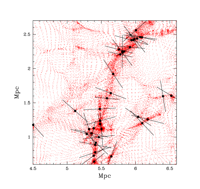
Figure 2 shows a region of size $2.1\,{\rm Mpc}$ and thickness $0.25\,{\rm Mpc}$ at redshift $z=4$ in the computational volume. We focus on a region containing a large-scale cosmological filament. The red dots represent the ${\rm P^{3}M}$ particles, the black dots indicate the positions of clusters identified by the friend-of-friend algorithm, and the bars indicate the direction of least resistance. These bars have equal length in 3D, but since they are seen in projection, they appear to have different lengths. There is clearly an overall tendency of the directions of least resistance to be aligned with each other, and to be perpendicular to the filament. Outflows propagating along these directions will transport energy and metal-enriched gas preferentially in low-density regions.

Figure 2.— Region of size $2.1\,{\rm Mpc}$ and thickness $0.25\,{\rm Mpc}$ centered on a large-scale filament, at redshift $z=4$. Red dots: ${\rm P^{3}M}$ particles; Black dots: halos. The lines indicate the directions of least resistance.

2.3.2 Expansion

The dynamical equations describing the evolution of the outflows are presented in full detail in Paper I. They are based on the original treatment of Tegmark et al. (1993), SBO1, and Scannapieco et al. (2002), and have been generalized to the case of anisotropic outflows. Here we present a review of the method.

The injection of thermal energy by SNe produces an outflow of radius $R$, which consists of a dense shell of thickness $R\delta$ containing a cavity. A fraction $1-f_{m}$, of the gas is piled up in the shell, while a fraction, $f_{m}$, of the gas is distributed inside the cavity. We normally assume that most of the gas is located inside a thin shell ($\delta\ll 1$, $f_{m}\ll 1$). This is called the thin-shell approximation.

The evolution of an outflow of radius $R$ and opening angle $\alpha$ expanding out of a halo of mass $M$ is described by the following system of equations,

$$\ddot{R} = {8\pi G(p-p_{\rm ext})\over\Omega_{b}H^{2}R}-{3\over R}(\dot{R}-HR)^{2}-{\Omega H^{2}R\over 2}-{GM\over R^{2}}\,,$$ (3)

$$\dot{p} = {L\over 2\pi R^{3}[1-\cos(\alpha/2)]}-{5\dot{R}p\over R}\,,$$ (4)

where a dot represents a time derivative, $\Omega$, $\Omega_{b}$, and $H$ are the total density parameter, baryon density parameter, and Hubble parameter at time, $t$, respectively. $L$ is the luminosity (see below), $p$ is the thermal pressure resulting from this luminosity, and $p_{\rm ext}$ is the external pressure of the IGM. $\alpha$ is the opening angle of the outflow, which is $180^{\circ}$ for isotropic outflows.

The external pressure $p_{\rm ext}$ depends upon the density and temperature of the IGM. As in Paper I, we assume a photoheated IGM made of ionized hydrogen and singly-ionized helium, with a fixed temperature $T_{\rm IGM}=10^{4}{\rm K}$ (Madau et al., 2001), and an IGM density $\rho^{\phantom{1}}_{\rm IGM}$ equal to the mean baryon density, $\bar{\rho}_{b}$. The external pressure is then given by

$$p_{\rm ext}(z)={\bar{\rho}_{b}kT_{\rm IGM}\over\mu}={3\Omega_{b,0}H_{0}^{2}kT_{\rm IGM}(1+z)^{3}\over 8\pi G\mu}\,,$$ (5)

where $z$ is the redshift and $\mu=0.611$ is the mean molecular mass.

The luminosity $L$ is the rate of energy deposition or dissipation within the outflow, and is given by

$$L(t)=L_{\rm SN}-L_{\rm comp}\,,$$ (6)

where $L_{\rm SN}$ is the total luminosity of the supernovae responsible for generating the outflow, and $L_{\rm comp}$ represents cooling due to Compton drag against CMB photons (other contributions are neglected, as in Paper I). The supernovae luminosity, for a galaxy forming in a halo of mass $M$, is given by

$$L_{\rm SN}={f_{\rm w}E_{0}\over t_{\rm burst}}{M_{*}\over M_{\rm req}}=2.86f_{\rm w}f_{*}\left({\Omega_{b,0}\over\Omega_{0}}\right)\left({M\over 1{\rm M}_{\odot}}\right)\,{\rm L}_{\odot}\,,$$ (7)

where $f_{*}$ is the star formation efficiency, $M_{*}=f_{*}M\Omega_{b,0}/\Omega_{0}$ is the total mass in stars formed during the starburst, $f_{\rm w}$ is the fraction of the total energy released that goes into the outflow, $M_{\rm req}$ is the mass of stars required to form one SN, and $E_{0}=10^{51}{\rm ergs}$ is the energy released by each of these SNe. As in Paper I, we take the values $f_{*}=0.1$, $M_{\rm req}=89.7{\rm M_{\odot}}$ (derived using a broken power-law IMF from Kroupa 2001), and the mass-dependent expression for $f_{\rm w}$ given by Scannapieco et al. (2002).

The Compton luminosity for a mixture of ionized hydrogen and singly-ionized helium is given by

$$L_{\rm comp}={2\pi^{3}\over 45}{\sigma_{t}\hbar\over m_{e}}\left({kT_{\gamma 0}\over\hbar c}\right)^{4}\left(1-\cos{\alpha\over 2}\right)(1+z)^{4}pR^{3}\,,$$ (8)

where $\sigma_{t}$ is the Thompson cross section, and $T_{\gamma 0}$ is the present CMB temperature. We used $T_{\gamma}=T_{\gamma 0}(1+z)$, which is valid over the range of redshifts we consider.

The expansion of the outflow is initially driven by the supernovae luminosity. After a time $t_{\rm burst}=5\times 10^{7}{\rm yr}$, the supernovae turn off, and the outflow enters the “post-supernova phase.” The pressure inside the outflow keeps driving the expansion, but this pressure drops since there is no energy input from supernovae. Eventually, the pressure will drop down to the level of the external IGM pressure. At that point, we assume that the expansion of the outflow will simply follow Hubble expansion.

2.3.3 Ram Pressure Stripping

As outflows propagate into the IGM, the expanding shells of swept-up gas may eventually hit halos. Following SB01 and Paper I, we assume that if an already formed galaxy is hit by an outflow, the cross section is too small for the impact to have any significant effect. If a halo that has not yet collapsed and formed a galaxy is hit, two things might happen. Either the ram pressure of the outflow will strip the halo of its baryonic content, preventing the formation of a galaxy, or else the halo will be enriched in metals by the outflow. The condition for stripping is

$$\left({l^{2}\over 4R^{2}}\right)M_{o}v_{o}\geq M_{b}v_{\rm esc},$$ (9)

where $M_{o}$ and $R$ the mass and radius of the shell, respectively, $v_{o}$ is the outflow velocity, $l$ and $M_{b}$ are the radius and baryonic mass of the halo being hit, and $v_{\rm esc}$ is the escape velocity from the halo. In Paper I, we used the spherical collapse model to estimate the radius $l$ at the time of the hit. This model predicts that halos expand, eventually turn around, and collapse to a point. This was straight forward in the Monte Carlo approach of Paper I. However, in the numerical approach used in this paper, we identify collapsed halos using the friend-of-friend algorithm, and these halos obviously have a finite size. Thus, the basic spherical model needs to be modified to account for the fact that real halos do not collapse down to a point, but instead contract by a factor of order 2 after turnaround, and reach virial equilibrium. We describe our modified spherical collapse model in Appendix B.

When the criterion for stripping is met, the halo is labeled as being stripped, and it will not form a galaxy. If the halo is not stripped, the outflow will deposit metals into the halo.

2.3.4 Metal Enrichment of Halos

We assume that halos start with metallicity of $\rm[Fe/H]=-3$, which is negligible for the purposes of calculating the halo cooling time. Once galaxies are formed, metals are produced at rate of $2{\rm M_{\odot}}$ per SN (Nagataki & Sato, 1998). Hence the mass of metals in the outflow is

$$M_{Z}=f_{\rm esc}{2{\rm M_{\odot}}\over M_{\rm req}}f_{*}{\Omega_{b,0}\over\Omega_{0}}M\,,$$ (10)

where $f_{\rm esc}$ is the fraction of ISM gas blown out with the outflow. We use the value $f_{\rm esc}=0.5$ taken from the numerical simulations of Mori et al. (2002). This mass of metals is distributed evenly throughout the volume of the outflow.

When an outflow strikes a halo and does not strip it, it modifies the metal content of the halo by depositing a fraction of its metals, $f_{\rm dep}V_{\rm overlap}/V_{\rm outflow}$, where $f_{\rm dep}$ is a mass deposition efficiency, which we set at $f_{\rm dep}=0.9$, and $V_{\rm overlap}$ is the volume of the outflow that overlaps with the halo. For details, we refer the reader to Paper I.

The radiative cooling rate increases with metallicity. So when a halo is enriched by metals, we recompute its cooling time, which determines when this halo will form a galaxy. This is the potential to “bring to life” dead halos. A halo that cannot become a galaxy because its cooling time exceeds the age of the universe might form a galaxy after all, if metal enrichment reduces the cooling time. It turns out to be a rare occurrence. In all the simulations we performed only several galaxies were formed this way, out of $20\,000-60\,000$ galaxies.

2.4. Metal Enrichment of the IGM

Stellar evolution in galaxies produces metals, that are then carried into the IGM by outflows. Of particular interest is the volume filling factor, that is, the fraction of the IGM, by volume, that has been enriched in metals by outflows. To calculate the volume filling factor, we cannot simply add up the final volumes of the outflows, and divide by the volume of the computational box. Intergalactic gas enriched by outflows will move with time as structures grow, and therefore regions that were never hit by outflows might end up containing metals.

We take this effect into account, by using a dynamic particle enrichment scheme that was developed by Germain et al. (2009). By combining the dumps produced by the $\rm P^{3}M$ code, which contains the position of the particles, with the positions, orientations, and radii of the outflows, we can find which particles are being hit by outflows, and at what redshift. We can then use a Smoothed Particle Hydrodynamics technique to estimate the volume filling factor at any redshift. A smoothing length $h$ is ascribed to each particle. We calculate $h$ iteratively by requiring that each particle has between $60$ and $100$ neighbors within a distance $1.7h$. We then treat each particle as an extended sphere of radius $1.7h$ over which it is considered to be spread. We then divide the computational volume into $N=256^{3}$ cubic cells. The cells that are covered by one or more enriched particles are then considered enriched. Notice that simply counting the number of enriched particles in each cell would fail in low-density regions, where the local particle spacing exceeds the cell size

Additionally, giving a smoothing length to each $\rm P^{3}M$ particle enables us to easily calculate the gas density in the center of each cell, using the standard SPH equation,

$$\rho({\bf r}_{g})=\sum_{i}m_{i}W({\bf r}_{g}-{\bf r}_{i},h_{i})\,,$$ (11)

where ${\bf r}_{i}$, $m_{i}$, and $h_{i}$ are the position, mass, and smoothing length of particle $i$, ${\bf r}_{g}$ is the position of a grid point, and $W$ is the smoothing kernel (see Monaghan 1992 for a detailed description of SPH). We will use this in § 3.2 below.

3. RESULTS

We performed a series of ten simulations: five with our galaxy formation scheme excluding suppression by photoionization heating, to produce results that can be compared with our results in Paper I, and a further five with this suppression as used in Pieri & Martel (2007). In each case we simulate outflows with opening angles $\alpha=60^{\circ}$, $90^{\circ}$, $120^{\circ}$, $150^{\circ}$, and $180^{\circ}$. This latter case corresponds to isotropic outflows.

3.1. Without Photoionization Suppresion

3.1.1 Volume Filling Factor

Figure 3 shows the evolution of the volume filling factor for the five opening angles considered. Enrichment starts at redshift $z\sim 12$ when the first galaxies form, and steadily increase with time, to reach $8-28\%$ by redshift $z=2$. The fraction increases with decreasing angle, at all redshifts. This differs from the results of Paper I, and clearly shows the importance of an accurate description of clustering. In Paper I, we found that the fraction was nearly constant, near 14%, for angles between $\alpha=180^{\circ}$ and $\alpha=100^{\circ}$, and then dropped down to $11\%$ at $\alpha=60^{\circ}$ (Fig. 8, bottom left panel, in Paper I).

Figure 3.— Volume filling factor versus redshift, with various opening angles, for simulations without photoionization suppression of galaxy formation.

Three distinct effects determined the overall volume filling factor in Paper I. These effects are still present here but their relative impact is changed. First, outflows are much more likely to overlap when the sources are highly clustered and this effect is diminished where outflows are anisotropic and aligned. Second, clustering makes it more likely that an expanding outflow will hit a pre-galactic collapsing halo, possibly resulting in gas stripping and preventing a galaxy from forming and producing its own outflow. Again the impact of this effect is diminished where outflows are anisotropic. Third, the volume of each outflow decreases with decreasing angle, the increase in radius not being enough to compensate for the smaller angle. The first two effects tend to increase the volume filling factor for anisotropic outflows and are sensitive to the level of galaxy clustering. The third effect tends to decrease the overall volume filling factor and is insensitive to the degree of clustering. Our results here show a more accurate and stronger degree of halo clustering, thus explaining the more marked impact of the first two effects with respect to the third. This also explains the small fractions we obtain in the isotropic case here ($8\%$ at $z=2$) by comparison to the equivalent result in Paper I.

Table 1Statistics of Enrichment and Hits Without Photoionization Suppresion

$\alpha$	$V_{\rm outflows}$	V.F.F.	$N_{\rm hit}$	$N_{\rm stripped}$	$N_{\rm outflows}$
$60^{\circ}$	0.388	0.277	$159\,957$	$145\,188$	$63\,015$
$90^{\circ}$	0.381	0.206	$192\,115$	$168\,365$	$52\,354$
$120^{\circ}$	0.369	0.155	$213\,846$	$178\,304$	$44\,399$
$150^{\circ}$	0.367	0.109	$231\,058$	$178\,781$	$38\,707$
$180^{\circ}$	0.369	0.081	$234\,365$	$165\,353$	$34\,324$

In Table 1, we list, for each opening angle, the total volume of the outflows, $V_{\rm outflows}$ (sum of all the volumes, ignoring overlap, in units of the box volume), the volume filling factor (V.F.F.) the number of halos hit and stripped ($N_{\rm hit}$, $N_{\rm stripped}$, respectively), and the number of outflows, $N_{\rm outflows}$, all at $z=2$. Comparing $V_{\rm outflow}$ with V.F.F. in Table 1, we clearly see that the effect of overlap is mild for small opening angles, but becomes very important for large ones. As the opening angle increases, there are more halos hit, more halos stripped, and as a result fewer galaxies are formed, producing fewer outflows. Going from $\alpha=60^{\circ}$ to $\alpha=180^{\circ}$, the number of outflows drops by a factor of 2. Despite this, though, their total volumes are comparable (0.388 vs. 0.369) since the volume per outflow is greater for outflows with larger opening angles.

In addition to the three effects described above we are also able to consider a fourth effect given the dynamical nature of our new simualtions. The matter enriched with metals moves as the simulation proceeds, and this motion modifies the volume filling factor. An isotropic outflow produced by a galaxy enriches matter that is located near the galaxy, and this matter is likely to later contract as it accretes over the cosmological structure hosting the galaxy. Highly anisotropic outflows travel larger distances, and might enrich matter located far from cosmological structures, and potentially expanding away from them.

Notice that the number of galaxies formed is significantly larger than in Paper I ($\sim 20\,000$ in a cosmological volume that was 40% larger). As we showed in Paper I, the Monte Carlo method underestimates the number of galaxies compared to either an N-body simulation or the Press-Schechter approximation (see Fig. 4 in Paper I). This provides additional motivation for performing a full cosmological simulation.

3.1.2 Distribution of Metal-Enriched Gas

Figure 4.— Slice (of comoving size $15\,{\rm Mpc}\times 15\,{\rm Mpc}$, and comoving thickness $0.1\rm{Mpc}$) of the computational volume for an opening angle $\alpha=180^{\circ}$, showing the evolution of the distribution of metals, for simulations without photoionization suppression of galaxy formation. The areas shown in green are enriched. The black dots represent the $\rm P^{3}M$ particles, and show the large-scale structures.

Figure 5.— Same as Figure 4 for an opening angle $\alpha=120^{\circ}$.

Figure 6.— Same as Figures 4 and 5 for an opening angle $\alpha=60^{\circ}$.

Figures 4–6 show slices of the computational volume at redshifts $z=4.98$, 4.00, 3.00, and 2.00, for opening angles $\alpha=180^{\circ}$, $120^{\circ}$, and $60^{\circ}$, respectively. At high redshift, metals are located in high-density regions where the sources are located. As time goes on, they eventually reach lower-density region, but never travel far enough to reach the deepest voids. Instead, even at $z=2$, all metals are found near dense structures like clusters and filaments.

Figure 7.— The number of enriched cells $N^{\prime}_{\rho}$ in the simulation volume at $z=2$ as a function of IGM density with various opening angles, for simulations without photoionization suppression of galaxy formation. Top panel: $N^{\prime}_{\rho}$ as a fraction of the number of cells at this density, $N_{\rho}$. Bottom panel: $N^{\prime}_{\rho}$ as a function of the total number of cells, $N$.

Figure 8.— Same as Figure 7, except that the number of enriched cells has been multiplied by the factor $f_{\rm outflow}(\alpha)\equiv N_{\rm outflow}(180^{\circ})/N_{\rm outflows}(\alpha)$, where $N_{\rm outflows}$ is given in Table 1. This isolates the impact of anisotropy on the regions enriched by individual outflows.

The main effect of narrowing the opening angle is to increase the volume over which metals are dispersed, as Figure 3 showed. Comparing Figures 4–6, it appears that both high- and moderately-low-density regions are affected. It is not obvious from these figures that anisotropic outflows enrich predominantly low-density regions. To investigate this issue, we calculated the density at each of the $N$ cells on the grid, using equation (11). We then binned these cells according to density, and counted in each bin the number of cells, $N_{\rho}$, and the number of enriched cells, $N^{\prime}_{\rho}$. From this, we calculated statistics of metal enrichment vs. density. The results are shown in Figure 7. The top panel shows $N^{\prime}_{\rho}/N_{\rho}$; this is effectively the probability of enriching a systems of a given density. The galaxies producing the outflows are located in high-density regions, hence these regions are favored over low-density ones, even with anisotropic outflows (such outflows will still enrich the gas located near the galaxies). The enrichment reaches 80% or more in high-density regions. The extent of enrichment increases with decreasing opening angle, at all densities, although this effect is most significant at lower densities. Going from $\alpha=180^{\circ}$ to $\alpha=60^{\circ}$, $N^{\prime}_{\rho}/N_{\rho}$ increases by a factor of 3.90 at $\log[\rho/\bar{\rho}]=-1$, 3.53 at $\log[\rho/\bar{\rho}]=0$, 1.75 at $\log[\rho/\bar{\rho}]=1$, 1.24 at $\log[\rho/\bar{\rho}]=2$, and 1.13 at $\log[\rho/\bar{\rho}]=3$.

The bottom panel shows the number of grid points enriched at a given overdensity as a fraction of the total number of cells, $N$. There are very few cells at densities below $\log[\rho/\bar{\rho}]=-1.2$, but about $\sim 10\%$ of these cells get enriched, explaining why $N^{\prime}_{\rho}/N$ becomes negligible while $N^{\prime}_{\rho}/N_{\rho}$ does not. The curves are very similar for all opening angles, except for the overall amplitude. Most enriched cells are located at low-densities in the range $\log[\rho/\bar{\rho}]=-1$ to 0, even though enrichment is less efficient in these regions compared to high-density ones. Even in the case of isotropic outflows most of metals are in underdense regions when considered by volume.

As the opening angle is reduced, outflows travel predominantly into low-density regions, and the number of outflows increases, because less stripping occurs. These two effects are acting in the same direction in low-density regions, while they are competing in high-density regions. To separate the two effects, we replotted in Figure 8 the same results as in Figure 7, but rescaled by the number of outflows. That is, we have multiplied the number of enriched cells $N^{\prime}_{\rho}$ by the factor $f_{\rm outflow}\equiv N_{\rm outflow}(180^{\circ})/N_{\rm outflows}(\alpha)$, where $N_{\rm outflow}$ can be read from the last column of Table 1. The top panel of Figure 8 is strikingly similar to the top panel of Figure 9 in Paper I. As the opening angle decreases, low-density regions are being enriched more, at the expense of high-density regions. However, the crossover happens at a higher density, $\rho/\bar{\rho}\approx 10$, compared to $\rho/\bar{\rho}\approx 2$ if we make a similar correction to $f_{\rm outflow}$ for Paper I. We attribute this difference to our dynamical treatment of metal enrichment. Enriched gas located in low-density regions can eventually move into higher-density regions as the system evolves.

3.2. With Photoionization Suppression

Table 2Statistics of Enrichment and Hits With Photoionization Suppresion

$\alpha$	$V_{\rm outflows}$	V.F.F.	$N_{\rm hit}$	$N_{\rm stripped}$	$N_{\rm outflows}$
$60^{\circ}$	0.301	0.189	$84\,599$	$80\,082$	$49\,276$
$90^{\circ}$	0.280	0.119	$107\,242$	$100\,410$	$39\,994$
$120^{\circ}$	0.255	0.079	$120\,593$	$110\,588$	$32\,773$
$150^{\circ}$	0.238	0.065	$126\,114$	$112\,347$	$27\,339$
$180^{\circ}$	0.223	0.047	$120\,717$	$103\,479$	$22\,992$

Figure 9.— Volume filling factor versus redshift, with various opening angles, for simulations with photoionization suppression of galaxy formation.

Figure 9 shows the evolution of the volume filling factor with the inclusion of photoionization suppression of galaxy formation as described in §2.2. By comparison with Figure 3, one can see that the volume filling factor remains unaffected until $z\approx 4$ and after this the extent of mechanical feedback is diminished. The volume filling factor continues to increase until $z\approx 3$ after which it actually begins to fall until the end of our simulations at $z=2$. This is a result of the dynamics included in our simulation, whereby gravitational attraction carries metal-enriched regions towards dense structures faster than outflows can carry them away from these structures. The final statistics of the suite of runs with photoionization suppression are shown in Table 2. The same notation as Table 1 is used and as before increasing opening angles leads to more outflows hitting halos, more stripping and so fewer galaxies (and so outflows).

As one can see by comparing Table 2 with Table 1, the introduction of photoionization suppression has the weakest impact for our smallest opening angle: the volume filling factor is 32% lower due photoionization heating in the for $\alpha=60^{\circ}$. However, the most pronounced impact occurs one of our intermediate models, $\alpha=120^{\circ}$ where the volume filling factor is 49% lower. The number of halos hit is also non-linear with opening angle, peaking at $\alpha=150^{\circ}$. It is also notable that the summed volume of all outflows $V_{\rm outflows}$ shows a clear decline with increasing opening angle, indicating that the fall in galaxy numbers with increasing opening angle dominates over the impact of the change in individual outflow volumes. As in the case without the inclusion photoionization suppression, the true model volume fraction shows a stronger opening angle dependence and this is a sign of reduced outflow overlap for more anisotropic outflows.

The density dependence of the volume filling factor is shown in Figure 10. These results are broadly similar to those for the suite of simulations without photoionization suppression (Figure 7). The values of $N^{\prime}_{\rho}/N$ are reduced in underdense regions ($\log[\rho/\bar{\rho}]<0$), but almost unaffected in very high-density regions ($\log[\rho/\bar{\rho}]>1$). In these high-density regions, outflows strongly overlap, and the removal of some of them by photoionization suppression does not prevent cells from being enriched.

Figure 10.— The number of enriched cells $N^{\prime}_{\rho}$ in the simulation volume at $z=2$ as a function of IGM density with various opening angles, for simulations with photoionization suppression of galaxy formation. Top panel: $N^{\prime}_{\rho}$ as a fraction of the number of cells at this density, $N_{\rho}$. Bottom panel: $N^{\prime}_{\rho}$ as a function of the total number of cells, $N$.

4. DISCUSSION

In Paper I, we described the evolution of anisotropic outflows and the enrichment of the IGM using a simple Monte Carlo method that was originally introduced by SB01. In this paper, we used cosmological N-body simulations to simulate the formation and evolution of large-scale structures in a more realistic way. The results obtained with both methods show interesting differences. In the Monte Carlo approach, the volume filling factors were largely independent of opening angle (Fig. 8, bottom-left panel of Paper I). Here were find a clear dependence on outflow anisotropy: the volume filling factor increases with decreasing opening angle, as Figures 3 and 9 showed.

In Paper I, we generated a Gaussian density field at high redshift, filtered it at various mass scales, and used the spherical collapse model to predict the location and collapse redshift of halos. Hence, the location of halos was predetermined by the initial conditions, and these locations did not change with time. Also, the density $\rho$ was determined by a nonlinear mapping of the initial density field. The density $\rho({\bf r})$ at a comoving position ${\bf r}$ was thus entirely determined by the initial density at that location. This approach has the advantage of simplicity, but does not constitute a full treatment of clustering.

This can have important consequences. Galaxies tend to be located inside larger cosmological structures, like filaments or pancakes. If several galaxies are located in a common structure, they can affect each other in two ways. First, the outflows might overlap, and second, if an outflow hits a halo that has not yet formed a galaxy, ram pressure stripping might prevent the galaxy from forming. These two effects are reduced when the outflows are anisotropic, because such outflows travel away from the cosmological structures, into low-density regions, and tend to avoid other galaxies and other outflows.

These effects were present in the Monte Carlo simulations (Fig. 8, bottom right panel of Paper I), however, they were not dominant. Instead they either approximately balanced the decline in individual outflow volumes for increasingly anisotropic outflows (down to opening angles of $\alpha=100^{\circ}$) or were dominated by them (opening angles from $\alpha=100^{\circ}$ to $\alpha=60^{\circ}$). The strength of clustering is much more apparent in the cosmological N-body simulations, and these effects now dominate. The higher level of clustering in the simulations here give greater weight to the impact of outflows that travel preferentially into low-density regions. Most results which are sensitive to this effect are all stronger here: the reduced outflow overlap, the reduced stripping of halos, the increased extent of enrichment in low-density regions. There is one aspect in which these results show a weaker signal of anisotropy than Paper I: the enrichment of overdense systems. In Paper I the fact that outflows travel into low-density regions resulted in a reduction in the physical extent of outflows in overdense regions, here however, anisotropic outflows increase the extent of outflows for densities all the way up to $\rho/\bar{\rho}\approx 10$. This a consequence of the dynamic nature of our N-body simulations. At the time of launching the outflow may expand into underdense regions but as the simulation progresses the gas enriched by the outflow is re-accreted onto overdense structures.

The impact of this accretion is also notable in the context of results from Oppenheimer et al. (2009). They find that understanding the accretion of outflow gas back onto galaxies plays an important role in galaxy assembly and the stellar mass function of galaxies by $z=0$. We find accretion of outflow gas onto large-scale structures plays an important role at $z>2$ and it seems likely that much of this gas continues its infall onto galaxies and fuels star formation.

Consider a galaxy producing an outflow that carries metals into low-density regions. As Figures 4–6 show, outflows never travel very far from their sources. Thus, the gas enriched by outflows is likely to be gravitationally bound to the structure hosting the galaxy. As that gas accretes onto that structure, it carries metals from a low- to a high-density region. This effect has been found by Germain et al. (2009) in a different context (anisotropic outflows powered by AGNs). As these authors argue, even though anisotropic outflows deposit metals predominantly in low-density regions, the subsequent evolution of the large-scale structure will tend to partly wash out that effect. The only exception might occur when outflows travel very large distances, reaching gas inside deep voids that is not destined to accrete onto any structure within a Hubble time. This happens with AGN-powered outflows (Germain et al., 2009), but SNe-powered outflows do not have enough energy to reach such distances.

The simulations presented in this paper use the same outflow model as the ones presented in Paper I. Only the method used for generating the population of halos (Monte Carlo vs. N-body simulations) and for calculating the enrichment of the IGM (static vs. dynamical) are different. The outflow model contains several parameters, such as $f_{*}$, $f_{\rm w}$, $f_{\rm esc}$, and $M_{\rm req}$. We use the same values as in Paper I, and we refer the reader to that paper for a discussion on the limits on these various parameters.

5. SUMMARY AND CONCLUSION

We have combined cosmological N-body simulations with a friend-of-friend algorithm for identifying halos and merger events, and an anisotropic outflow model, to study the metal-enrichment of the IGM by SNe-powered galactic outflows, in a $\Lambda$CDM universe. Outflows are modeled as bipolar cones traveling along the direction of least resistance, which we take as the direction along which the density drops the fastest. We performed five simulations with outflow opening angles ranging from $60^{\circ}$ to $180^{\circ}$, the latter case corresponding to isotropic outflows. Each simulation was stopped at redshift $z=2$. For each simulation, we tracked the deposition of metals in the IGM by outflows, and the subsequent motion of the metal-enriched gas. We also included the effect of ram pressure stripping and metal enrichment of pre-galactic collapsing halos that are hit by outflows. We did this with and without the inclusion of photoionization suppression of galaxy formation resulting in a total of ten simulations. Our main results are the following.

• Anisotropic outflows travel predominantly into low-density regions, away from cosmological structures (filament and pancakes) that host most galaxies. As a result, anisotropic outflows are less likely to overlap than isotropic ones, and are less likely to inhibit galaxy formation by stripping collapsing halos of their gas. The combination of these effect results in an increase of the volume filling factor of the IGM with decreasing opening angle, from 8% with isotropic outflows, up to 28% with opening angle of $60^{\circ}$.

• The majority of collapsing halos hit by outflows end up being stripped of their gas, preventing the formation of a galaxies. The total number of galaxies formed drops by a factor of 2 when going from opening angle $\alpha=60^{\circ}$ to $180^{\circ}$. Halos not stripped are enriched in metals, with negligible consequences for the formation time of the galaxy. In particular, fewer than one in $10^{3}-10^{4}$ galaxies that formed would not have formed without the hit, because their cooling time exceeded the Hubble time.

• The volume filling factor remain small (28% or less) because outflows do not travel large distances. They remain fairly close to the structures where they originate, never reaching the center of the deep cosmological voids. The regions most efficiently enriched (up to 90% by volume) are the high-density regions, where the galaxies producing the outflows are located. The enrichment of low-density regions is not as efficient. However, by volume, most metals are located in these low-density region, because their combined volume greatly exceeds the combined volume of high-density regions. Indeed, most of the enriched volume is in regions whose density is between $0.1\bar{\rho}$ and $\bar{\rho}$.

• As outflows become more anisotropic (smaller opening angle $\alpha$), the extent of enrichment increases at all densities, low and high. The effect is most important at low densities, where the efficiency increases by factors of several. At very-high densities, $\rho=1000\bar{\rho}$, regions are already 80% enriched by volume by isotropic outflows, so there is little room for an additional increase.

• Overall, anisotropic outflows do not strongly favor low-density regions at the expense high-density ones, unlike what was found in Paper I. Anisotropic outflows are more numerous, resulting in higher probability of enrichment at all densities. When this effect is factored-out, we find that the probability that a galaxy will enrich systems at densities up to $10\bar{\rho}$ is higher for increasingly anisotropic outflows. This results from evolution of the metal-enriched IGM. Enriched gas tends to be located relatively near the large-scale structures hosting the galaxies responsible for this enrichment. As that enriched gas accretes onto these structures, the effect of anisotropy is partly washed out.

• Photoionization suppression of low-mass galaxy formation leads to a number of modifications to our enrichment predictions. Since many of these low mass galaxies would otherwise have formed in or near voids of our density distribution, their suppression leads to a reduction in the enrichment of low-density regions. Also a surprising, but not implausible, consequence of this prescription is a fall in volume fraction of enriched regions after $z=3$. This is a consequence of suppression of much late galaxy formation combined with the accretion of enriched structures back onto high-density, low-volume regions.

Appendix A MERGER TREE: DEALING WITH SPLITTERS

While building merger trees, we discovered that some clusters of ${\rm P^{3}M}$ particles were actually splitting, that is, breaking up into two or more components. Such splitting might be real. A small cluster located in the vicinity of a larger one might get stretched by the tidal field to the point where it breaks up, or it might get so elongated that the FOF algorithm identifies it as several clusters. This can also be a purely numerical effect, which could occur in two different situations: (1) Two clusters that pass near each others without merging come briefly into contact. If the FOF algorithm is applied while the clusters are in contact, they will be identified as one single cluster, that then splits. (2) When two clusters approach each others on a collision course, they will be identified as one single cluster as soon as one particle from the first cluster and one particle from the other cluster are within a linking length of one another. Then, because of the internal motion of the particles inside clusters, the two clusters might lose and re-establish contact several times during the following timesteps, before they finally merge for good. These effects are artifacts of the FOF algorithm, and usually go unnoticed unless one uses a very fine time resolution when building merger trees. In this paper, we build cluster catalogs spaced by time intervals of $2.5\times 10^{7}{\rm years}$, which gives us merger trees with 306 levels between redshift $z=6$ and $z=2$. With such a fine time resolution, these ‘splitters’ become a real problem, which needs to be addressed. More specifically, since mergers result in starburst, we have to be sure that mergers identified by the FOF algorithm are real. A merger that immediately follows or is immediately followed by a splitter might not be real.

Figure 11.— Contour plot showing the time $t_{\rm sur}$ that a merger remnant survives before it splits, vs. the time $t_{\rm ret}$ that a split lasts before the various parts re-merge together. The contours show the number of clusters. All clusters have either $t_{\rm sur}<t_{\rm stab}$, $t_{\rm ret}<t_{\rm stab}$, or both, where $t_{\rm stab}=1.5\times 10^{8}{\rm years}$ is the time of stability.

We have designed an algorithm that scans our merger trees and eliminate splitters that appear to be spurious. We start by defining a time of stability $t_{\rm stab}$, which is the minimum time a cluster must exist in the simulation to be considered a real cluster. When a cluster forms by a merger, and then splits, we calculate the time $t_{\rm sur}$ during which the cluster survived before splitting. If $t_{\rm sur}<t_{\rm stab}$, we consider that the cluster was not present long enough to be considered real, and therefore the merger that formed that cluster and the subsequent splitter that destroyed it were both spurious. This handles the first case described above, that is of two clusters that briefly come into contact during a non-merging encounter.

This leaves the second case, two clusters that experience a series of mergers and splitters before finally merging for good. In this case, every time the cluster splits, the two pieces will re-merge after a time $t_{\rm ret}$. If this time is sufficiently short, we assume that the split and the subsequent re-merging were spurious, and that the cluster actually never split. We use the criterion $t_{\rm ret}<t_{\rm stab}$, where $t_{\rm stab}$ is the time of stability that was used in the other criterion.

We have applied this method to the merger tree built from our simulation, using a time of stability $t_{\rm stab}=1.5\times 10^{8}{\rm years}$. We have identified all cases where a cluster splits. For each case, we calculated the time $t_{\rm sur}$ during which the cluster existed before it split, and the time $t_{\rm ret}$ elapsed before the various pieces re-merged together (this can be infinite if the pieces never re-merged). In Figure 11, we show a plot of $t_{\rm ret}$ vs. $t_{\rm sur}$, where the contours show the actual number of clusters. Most clusters have either $t_{\rm sur}<t_{\rm stab}$, $t_{\rm ret}<t_{\rm stab}$, or both. Hence, according to our criterion, these splitters are not real, and we simply ignore them. A small fraction of splitters fail both criteria, and are considered real splitters. Such splitters occur when a small halo is torn apart by the tidal field of a larger one. This violent process should result in a significant reheating of the gas, which can later cool down and lead to a starburst. Consequently, we treat a halo formed by a splitter like we treat halos formed by monolithic collapse and mergers: we calculate its cooling time, and after that time has elapsed, we start a new outflow. Note that the details of this treatment are not critical, since real splitters are rare.

Appendix B THE SPHERICAL COLLAPSE MODEL

In SB01 and Paper I, the spherical top-hat collapse model was used to estimate the size of uncollapsed halos when these halos are hit by outflows. The comoving radius of a halo is given by

$$l=\left({2\over 9}\right)^{1/3}\!{R(1-\cos\theta)\over(\theta-\sin\theta)^{2/3}}\,,$$ (B1)

where $R$ is the comoving radius in the limit $z\rightarrow\infty$. In equation (B1), the parameter $\theta$ is obtained by solving the following transcendental equation,

$$\left({\theta-\sin\theta\over 2\pi}\right)^{2/3}={\delta_{+}(z)\over\delta_{+}(z_{\rm coll})}\,,$$ (B2)

where $\delta_{+}$ is the linear growing mode. As $z$ varies from $z=\infty$ to $z=z_{\rm coll}$, $\theta$ varies from 0 to $2\pi$. The physical radius of the halo is given by

$$l_{\rm phys}=\left({2\over 9}\right)^{1/3}\!{R(1-\cos\theta)\over(1+z)(\theta-\sin\theta)^{2/3}}\,.$$ (B3)

Notice that at high redshift (when $\Omega\approx 1$ and $\lambda\approx 0$), $\delta_{+}(z)\approx(1+z)^{-1}$. Hence, the denominator in equation (B3) is nearly constant. The time-dependence in equation (B3) essentially comes from the factor $(1-\cos\theta)$ in the numerator. The halo has a physical size of 0 at $\theta=0$ (corresponding to the big bang), reaches maximum size at $\theta=\pi$, and collapses to a black hole at $\theta=2\pi$.

In practice, halos will not collapse to a black hole. After turnaround, radial motions will be converted into transverse motions, and eventually the halo will virialize, with a physical radius that is 1/2 of the maximum physical radius (that is, the halo shrinks by a factor of 2 in radius after turnaround). We do not have a precise model for the evolution of the system between turnaround and virialization. A fair assumption is that the time it takes for the halo to shrink by a factor of 2 is equal to the time it would have taken to collapse to a black hole in the absence of virialization (Padmanabhan 1993; Dekel & Ostriker 1999; see however Coles & Lucchin 1995). To achieve this result, we modify equation (B1) and (B3), using

$$l = \left({2\over 9}\right)^{1/3}{R\chi(\theta)\over(\theta-\sin\theta)^{2/3}}\,,$$ (B4)

$$l_{\rm phys} = \left({2\over 9}\right)^{1/3}\!{R\chi(\theta)\over(1+z)(\theta-\sin\theta)^{2/3}}\,,$$ (B5)

where

$$\chi(\theta)=\cases{1-\cos\theta\,,&$\theta\leq\pi$;\cr\vskip 6.0pt plus 2.0pt minus 2.0pt\cr\displaystyle{1\over 2}(3-\cos\theta)\,,&$\theta>\pi$.\cr}$$ (B6)

Figure 12.— Evolution of a spherical halo collapsing at redshift $z_{\rm coll}=3$ in a universe with $\Omega_{0}=0.268$ and $\lambda_{0}=0.732$. The solid and dashed curves show the standard and modified spherical collapse model, respectively.

Figure 12 shows the evolution of a spherical halo collapsing at redshift $z_{\rm coll}=3$ in a universe with $\Omega_{0}=0.268$ and $\lambda_{0}=0.732$. The comoving radius and physical radius are plotted versus time in units of the Hubble time $1/H_{0}$. Since the evolution is similar for halos of different sizes, we set arbitrarily $R=1$. The solid curves show the basic spherical model given by equations (B1), (B2) and (B3). The dashed curves show the effect of using equation (B4) and (B5). After turnaround, the halo collapses by a factor close to 2.

It is convenient to re-express the physical radius in terms of its final value at $z=z_{\rm coll}$. That value is obtained by setting $z=z_{\rm coll}$ and $\theta=2\pi$ in equation (B5). We get

$$l_{\rm phys}(z)=l_{\rm phys}(z_{\rm coll})\biggl{[}{(1+z_{\rm coll})\delta_{+}(z_{\rm coll})\over(1+z)\delta_{+}(z)}\biggr{]}^{2/3}\chi(\theta)\,.$$ (B7)

Since at high redshift the quantity in brackets is close to unity, the time-dependence is essentially given by the function $\chi(\theta)$.

References

- Aguirre et al. (2001) Aguirre, A., Hernquist, L., Schaye, J., Katz, N., Weinberg, D. H., & Gardner, J. 2001, ApJ, 561, 521
- Aguirre et al. (2008) Aguirre, A., Dow-Hygelund, C., Schaye, J., & Theuns, T. 2008, ApJ, 689, 851
- Barai et al. (2010) Barai, P., Martel, H., & Germain, J. 2010, submitted to ApJ
- Bertone et al. (2005) Bertone, S., Stoehr, F., & White, S. D. M. 2005, MNRAS, 359, 1201
- Bland & Tully (1988) Bland, L., & Tully, R. B. 1988, Nature, 334, 43
- Coles & Lucchin (1995) Coles, P., & Lucchin, F. 1995, Cosmology. The Origin and Evolution of Cosmic Structure (New York: Wiley)
- Davis et al. (1985) Davis, M., Efstathiou, G., Frenk, C. S., & White, S. D. M. 1985, ApJ, 292, 371
- Dekel & Ostriker (1999) Dekel, A., & Ostriker, J. P. 1999, Formation of Structure in the Universe (Cambridge University Press).
- Dijkstra et al. (2004) Dijkstra, M., Haiman, Z., Rees, M. J., & Weinberg D. H., ApJ, 601, 666
- Eke et al. (1996) Eke, V. R., Cole, S., & Frenk, C. S. 1996, MNRAS, 282, 263
- Fabbiano et al. (1990) Fabbiano, G., Heckman, T., & Keel, W. C. 1990, ApJ, 355, 442
- Germain et al. (2009) Germain, J., Barai, P., & Martel, H. 2009, ApJ, 704, 1002
- Hockney & Eastwood (1981) Hockney, R. W., & Eastwood, J. W. 1981, Computer Simulation using Particles (New York: McGraw Hill).
- Kroupa (2001) Kroupa, P. 2001, MNRAS, 322, 231
- Mac Low & Ferrara (1999) Mac Low, M.-M., & Ferrara, A. 1999, ApJ, 513, 142
- Madau et al. (2001) Madau, P., Ferrara, A., & Rees, M. J. 2001, ApJ, 555, 92
- Martel & Shapiro (2001a) Martel, H., & Shapiro, P. R. 2001a, Rev.Mex.A&A (SC), 10, 101
- Martel & Shapiro (2001b) Martel, H., & Shapiro, P. R. 2001b, in Relativistic Astrophysics, AIP Conference Proceedings 586, eds. J. C. Wheeler & H. Martel, p. 265
- Meyer & York (1987) Meyer, D. M., & York, D. G. 1987, ApJ, 315, L5
- Monaghan (1992) Monaghan, J. J. 1992, ARA&A, 30, 543
- Mori et al. (2002) Mori, M., Ferrara, A., & Madau, P. 2002, ApJ, 571, 40
- Nagataki & Sato (1998) Nagataki, S., & Sato, K. 1998, ApJ, 504, 629
- Oppenheimer & Davé (2006) Oppenheimer, B. D., & Davé, R. 2006, MNRAS, 373, 1265
- Oppenheimer et al. (2009) Oppenheimer, B. D., Davé, R., Kereš, D., Fardal, M., Katz, N., Kollmeier, J. A., & Weinberg, D. H. 2009, submitted to MNRAS, (astro-ph.CO/0912.0519)
- Padmanabhan (1993) Padmanabhan, T. 1993, Structure Formation in the Universe (Cambridge University Press).
- Pieri & Haehnelt (2004) Pieri, M. M., & Haehnelt, M. G. 2004, MNRAS, 347, 985
- Pieri & Martel (2007) Pieri, M. M., & Martel, H. 2007, ApJ, 662, L7
- Pieri et al. (2007) Pieri, M. M., Martel, H., & Grenon, C. 2007, ApJ, 658, 36 (Paper I)
- Pieri et al. (2006) Pieri, M. M., Schaye, J., & Aguirre, A. 2006, ApJ, 638, 45
- Pieri et al. (2009) Pieri, M. M., Frank, S., Mathur, S., Weinberg, D., H., York, D. G., & Oppenheimer, B., D. 2009, submitted to ApJ, (astro-ph.CO/0908.2001)
- Pieri et al. (2010) Pieri, M. M., Frank, S., Mathur, S., Weinberg, D., H., & York, D. G. 2010, submitted to ApJL, (astro-ph.CO/1001.5282)
- Scannapieco & Broadhurst (2001) Scannapieco, E., & Broadhurst, T. 2001, ApJ, 549, 28 (SB01)
- Scannapieco et al. (2002) Scannapieco, E., Ferrara, A., & Madau, P. 2002, ApJ, 574, 590
- Scannapieco et al. (2001) Scannapieco, E., Thacker, R. J., & Davis, M. 2001, ApJ, 557, 605
- Schaye et al. (2003) Schaye, J., Aguirre, A., Kim, T., Theuns, T., Rauch, M., & Sargent, W. L. W. 2003, ApJ, 596, 768
- Shopbell & Bland-Hawthorn (1998) Shopbell, P. L., & Bland-Hawthorn, J. 1998, ApJ, 493, 129
- Spergel et al. (2007) Spergel, D. N. et al. 2007, ApJS, 170, 377
- Springel & Hernquist (2003) Springel, V., & Hernquist, L. 2003, MNRAS, 312, 334
- Strickland et al. (2000) Strickland, D. K., Heckman, T. M., Weaver, K. A., & Dahlem, M. 2000, AJ, 120, 2965
- Tegmark et al. (1993) Tegmark, M., Silk, J., & Evrard, A. 1993, ApJ, 417, 54
- Theuns et al. (2001) Theuns, T., Mo, H. J., & Schaye, J. 2001, MNRAS, 321, 450
- Theuns et al. (2002a) Theuns, T., Schaye, J., Zaroubi, S., Kim, T.-S., Tzanavaris, P., Carswell, R. F. 2002a, ApJ, 567, L103
- Theuns et al. (2002b) Theuns, T, Viel, M., Kay, S., Schaye, J., Carswell, R. F., & Tzanavaris, P. 2002b, ApJ, 578, L5
- Veilleux & Rupke (2002) Veilleux, S., & Rupke, D. S. 2002, ApJ, 565, L63
- White & Frenk (1991) White, S. D. M., & Frenk, C. S. 1991, ApJ, 379, 52