Habitable Climates: The influence of eccentricity

Abstract

In the outer regions of the habitable zone, the risk of transitioning into a globally frozen “snowball” state poses a threat to the habitability of planets with the capacity to host water-based life. Here, we use a one-dimensional energy balance climate model (EBM) to examine how obliquity, spin rate, orbital eccentricity, and the fraction of the surface covered by ocean might influence the onset of such a snowball state. For an exoplanet, these parameters may be strikingly different from the values observed for Earth. Since, for constant semimajor axis, the annual mean stellar irradiation scales with $(1-e^{2})^{-1/2}$, one might expect the greatest habitable semimajor axis (for fixed atmospheric composition) to scale as $(1-e^{2})^{-1/4}$. We find that this standard simple ansatz provides a reasonable lower bound on the outer boundary of the habitable zone, but the influence of both obliquity and ocean fraction can be profound in the context of planets on eccentric orbits. For planets with eccentricity 0.5, for instance, our EBM suggests that the greatest habitable semimajor axis can vary by more than 0.8 AU (78%!) depending on obliquity, with higher obliquity worlds generally more stable against snowball transitions. One might also expect that the long winter at an eccentric planet’s apoastron would render it more susceptible to global freezing. Our models suggest that this is not a significant risk for Earth-like planets around Sun-like stars, as considered here, since such planets are buffered by the thermal inertia provided by oceans covering at least 10% of their surface. Since planets on eccentric orbits spend much of their year particularly far from the star, such worlds might turn out to be especially good targets for direct observations with missions such as TPF-Darwin. Nevertheless, the extreme temperature variations achieved on highly eccentric exo-Earths raise questions about the adaptability of life to marginally or transiently habitable conditions.

1. Introduction

There are now more than 460 extrasolar planets known. Selection effects favor the discovery of massive giant planets orbiting very close to their parent stars, but advances in imaging and spectroscopic capabilities, longer baselines for observation, and missions such as CoRoT and Kepler should accelerate the rate of discovery of less massive planets in longer period orbits in the near future. In particular, microlensing observations have already detected planets less than ten times as massive as the Earth at distances as great as 2.6 AU (Beaulieu et al., 2006; Bennett et al., 2008), and have discovered a potential analog to our solar system (Gaudi et al., 2008) that might allow a habitable planet on a stable orbit (Malhotra & Minton, 2008). Both CoRoT and Kepler promise to further increase the number of detected terrestrial exoplanets (Baglin, 2003; Borucki et al., 2003, 2007; Borucki & for the Kepler Team, 2010). The observed secondary eclipse of HAT-P-7b by Kepler demonstrates that it should be capable of detecting transits of Earth-size planets (Borucki et al., 2009). Additionally, the CoRoT team recently announced the detection of the $\sim$1.7$R_{\earth}$ exoplanet COROT-Exo-7b orbiting a K0 star in the constellation Monoceros (Rouan et al., 2009; Leger et al., 2009; Bouchy et al., 2009; Fressin et al., 2009) and the MEarth Project detected the transit of the 6.55 M_⊕ planet GJ 1214b (Charbonneau et al., 2009). Although these planets are in extremely close orbits ($a=0.017$ AU, P = 0.85 days for COROT-Exo-7b; $a=0.014$ AU, P = 1.58 days for GJ 1214b) and are unlikely to be habitable, their discoveries represent a tremendous advance in planet detection capability. As the CoRoT, Kepler, and MEarth projects continue, even less massive terrestrial planets will surely be discovered in orbits with greater semimajor axes. Once these potentially habitable terrestrial planets are discovered, researchers will be able to determine the radii, orbital semimajor axes, and masses of the planets, but current techniques are insufficient to constrain their obliquities and rotation rates (Valencia et al., 2006, 2007; Adams et al., 2008). Although transit measurements might place constraints on the eccentricities of some transiting planets (Barnes, 2007; Ford et al., 2008), radial velocity measurements of exact Earth analogs will be extremely challenging, and so the eccentricities of most such planets will remain undetermined in the near future. This paper attempts to quantify the effects of orbital parameters such as eccentricity on planetary habitability in order to prepare us to draw inferences about the habitability of yet-to-be-detected terrestrial planets even if their eccentricities are not well constrained.

However, current surveys of extrasolar planets indicate that the near-zero eccentricities seen in the Solar System are not necessarily typical and that many planets have significantly higher eccentricities (Udry & Santos, 2007). Of the exoplanets with measured eccentricities, $\sim$40% are on more eccentric orbits than Pluto (${e=0.2488}$) and $\sim$10% are on orbits with eccentricities $>$0.5. This suggests that current views of habitability that focus on direct Earth analogs in near-circular orbits might consider only a small subset of potentially habitable worlds. It therefore seems prudent to expand our study of habitability to encompass a wide range of orbital parameters.

The study of planetary habitability began decades prior to the detection of exoplanets with the classic work of Dole (1964) and Hart (1979). In the last two decades, this topic has been revisited with increasing frequency, beginning with the work of Kasting et al. (1993), who found conservative limits for the Earth’s liquid water habitable zone between 0.95 AU and 1.37 AU. In recent years, various studies have applied the tools and techniques used to study the Earth’s climate to simulations of planets around other stars. Investigations by Williams & Pollard (2003), Williams & Kasting (1997) and Spiegel et al. (2009) have shown that, while variations in the polar obliquity angle can alter the distance from the star at which a planet becomes too cold to be habitable, planets with high obliquities are not necessarily less habitable than planets with low obliquities. Williams & Pollard (2002) also considered the effect of eccentricity on habitability but only in the context of Earth twins at 1 AU.

Spiegel et al. (2008, 2009) have analyzed the effect of changes in semimajor axis, rotation rate, obliquity, and ocean coverage on the temperature of a generic terrestrial planet, but not variations in eccentricity. This paper attempts to fill in the void between the work of Spiegel et al. (2009) and Williams & Pollard (2002) by varying the eccentricity of model planets that are more diverse than the Earth-twin used by Williams & Pollard (2002). In addition, we also conduct a sensitivity study to determine which parameters have the strongest effect on planetary temperatures, so as to quantify the degree to which uncertainty in parameter measurement translates to uncertainty in climate.

Although some planets may be habitable at all latitudes during their entire orbit, other planets, like the Earth, might be only partially habitable. These planets could therefore transition to a “snowball state” if small changes in insolation or atmospheric composition cause part or all of the planet to freeze. During a “snowball transition,” the formation of snow or ice increases the albedo of the planet and the planet consequently becomes even colder. If the positive feedback loop between ice formation and increased albedo continues, the entire planet may become frozen and trapped in a snowball state. As discussed in Section 5.1, the accumulation of greenhouse gases in the atmosphere while the planet is frozen may warm the surface sufficiently to allow the planet to eventually exit the snowball state. The transition from a snowball state to a partially habitable state is beyond the scope of this paper, but an investigation is pursued in Pierrehumbert (2005) as well as in a companion paper (Spiegel et al., 2010).

In this paper, based on a simple energy balance model (EBM) treatment, we determine that obliquity, eccentricity, and ocean fraction can together have a very strong influence on the orbital location of the snowball transition. For instance, for models with an Earth-like atmosphere and eccentricity 0.5 (which might not be extreme by extrasolar standards), we find that the maximum habitable semimajor axis can extend to 1.90 AU or be as close to the star as 1.07 AU, depending on obliquity and ocean fraction. As a result, for $e=0.5$, the standard ansatz for the outer boundary of the habitable zone derived from considering only the annual mean flux (Barnes et al., 2008) can be off by more than 78%. Altering the azimuthal obliquity (the degree of alignment of periastron with the solstices) does not have a significant effect on where the snowball transition occurs for low eccentricity planets, but the transition for high eccentric planets is pushed out significantly for azimuthal obliquity $\sim$30^∘. More generally, planets in higher eccentricity orbits display more latitudinal variation and seasonal variation in habitability than planets in near-circular orbits. Because all of the models in this study incorporate an Earth-like atmosphere, simultaneous variations of atmospheric composition or other factors in combination with the parameters considered in this study may produce a more complicated picture of general planetary habitability.

In Section 2 we discuss several important factors that influence the Earth’s climate on long time-scales. We explain the setup of our model in Section 3 and discuss the validation of the model in Section 4. In Section 5 we present our results. We then conclude in Section 6 and consider the implications of our findings on planetary habitability.

2. Generalized Milankovitch Cycles

Milankovic (1941) realized that the long-term climate behavior of the Earth could in part be explained by considering the combined effects of obliquity, orbital eccentricity, and precession. Each of these orbital elements changes on multiple, nonconstant timescales known as Milankovitch cycles and the combination of these variations alters the climate of the Earth by increasing or decreasing the solar insolation received by the Earth at a given latitude. For example, increasing the Earth’s obliquity increases the annually averaged insolation received by the poles and decreases the annually averaged insolation received by the equator; both effects act to decrease the latitudinal temperature gradient.” However, the Earth’s obliquity is largely stabilized by the Moon and varies by only ${\pm 1.2^{\circ}}$ on timescales of $\sim$41 kyr (Laskar et al., 1993; Berger, 1976, 1978). Much higher variations in obliquity are expected for planets without large moons: the obliquity of Mars varies between ${14.9^{\circ}}$ and ${35.5^{\circ}}$ (Ward, 1974) and numerical models suggest that the Earth would experience obliquity oscillations between ${0^{\circ}}$ and ${85^{\circ}}$ in the absence of the Moon (Laskar et al., 1993; Laskar & Robutel, 1993). Even in the absence of large moons, however, the obliquity of a quickly rotating planet ($\lesssim$8-hour day) would probably be self-stabilized by the fast rotation rate of the planet (Ward, 1982; Laskar et al., 1993).

In addition to obliquity, there is also a Milankovitch cycle governing precession on shorter timescales of $\sim$19 kyr and $\sim$23 kyr (Berger, 1976, 1978). Over time, the slow shift of the direction of the Earth’s rotation axis due to precession of both the spin axis and the orbital ellipse alters the position of solstices and equinoxes with respect to apoastron and periastron. In this paper, we consider this effect by varying the azimuthal obliquity angle $\theta_{a}$ of our model planets (defined in Section 3 as the angle between the position of the planet at periastron and the position of the planet at the northern winter solstice). Due to the ice albedo effect, the hemisphere that is tilted toward the star at apoastron—which has a shorter winter (i.e., a shorter period of high albedo)—absorbs more integrated stellar energy per year than does the hemisphere that is tilted away at apoastron. Accordingly, the greatest temperature asymmetry between the northern and southern hemispheres is produced when periastron is aligned with a solstice (${\theta_{a}=0^{\circ}}$ or ${\theta_{a}=180^{\circ}}$). Conversely, both hemispheres absorb equal annually averaged stellar irradiation when periastron is aligned with an equinox (${\theta_{a}=90^{\circ}}$ or ${\theta_{a}=270^{\circ}}$).

Finally, there is a Milankovitch cycle for eccentricity. The Earth’s orbital eccentricity is currently nearly circular (${e=0.0167}$), but varies slowly up to $\sim$0.06 over long timescales of $\sim$100 and $\sim$400 kyr (Berger, 1976, 1978). As shown in Figure 2, the annual mean flux ${\left<F\right>}$ scales as ${(1-e^{2})^{-1/2}}$ so that flux increases with increasing eccentricity for a given semimajor axis. Increasing the eccentricity, therefore, accentuates the ratio of the irradiating flux at periastron to that at apoastron (${F_{\rm max}/F_{\rm min}\propto((1+e)/(1-e))^{2}}$), and slightly increases the annually averaged irradiation. The ratio ${F_{\rm max}/F_{\rm min}}$ can be quite substantial for highly eccentric orbits, exceeding $10^{2}$ for $e>0.82$, which could, depending on a planet’s thermal inertia and redistribution of energy, cause dramatic seasonal temperature swings. We present climate models of planets with high orbital eccentricity in Section 5.1, and refer readers to a companion paper (Spiegel et al., 2010) for a discussion of scenarios in which the eccentricity of an Earth-like planet might be excited to large values.

Over time, the combined changes in obliquity, precession, and eccentricity, together with nonlinear amplifications, can dramatically alter an exo-Earth’s climate, leading alternately to periods of glaciation and of deglaciation as has been shown in the case of the Earth (Berger et al., 2005; Crucifix et al., 2006; Laskar et al., 1993; Loutre et al., 2004; Quinn et al., 1991).

3. Model Setup

In this study, we investigate the temperature of a planet using the same one-dimensional time-dependent energy balance model introduced in Spiegel et al. (2008) and further explored in Spiegel et al. (2009). The model, which is similar to the more Earth-centric model used by Suarez & Held (1979), treats the meridional transport of heat as diffusion driven by the zonal mean temperature gradient:

$$C\frac{\partial T[x,t]}{\partial t}-\frac{\partial}{\partial x}\left(D(1-x^{2})\frac{\partial T[x,t]}{\partial x}\right)+I=S(1-A)\,.$$ (1)

This equation describes the evolution of the temperature $T$ at location $x\equiv\sin\lambda$, where $\lambda$ is the latitude, as a function of an effective heat capacity $C$, a diffusion coefficient $D$, and an albedo $A$. The net radiative energy flux in a latitude band is determined by the relationship between the energy received due to the diurnally averaged stellar flux $S$ and the energy lost due to infrared emission $I$. One-dimensional EBMs such as this model provide a reasonable approximation of seasonal mean temperatures for planets that rotate sufficiently quickly relative to their orbital frequency (Showman et al., 2009). In all of our models we assume that the planet orbits a Sun-like star, so the stellar flux $S$ is equivalent to that from a 1 $M_{\sun}$, 1 $L_{\sun}$ star. The effective heat capacities of the atmosphere over land ($C_{l}$), over the wind-mixed surface layer of the ocean ($C_{o}$), and over ice ($C_{i}$) are the same as in Spiegel et al. (2008, 2009) and Williams & Kasting (1997) and are shown in Table 1.

Previous work (Spiegel et al., 2008) explored three sets of infrared cooling radiation functions and albedo functions. Of the three models tested in that paper, Model 2 produced climates most similar to those on current Earth and is the one used in the current study:

$$I[T]=\frac{\sigma T^{4}}{1+0.5925\left(\frac{T}{273\mathrm{\ K}}\right)^{3}}\,\,,$$ (2)

where $\sigma$ is the Stefan-Boltzmann constant. The denominator of equation 2 would instead be 1 if the atmosphere had no opacity to outgoing infrared radiation; the functional form used for this denominator represents the strength of the greenhouse effect, and is a reasonable approximation of the greenhouse for present-Earth conditions (Spiegel et al., 2008). In order to account for the higher reflectivity of ice and snow while using a simple functional form, we take the albedo to be constant and low ($\sim$0.28) at high temperatures, constant and high ($\sim$0.77) at low temperatures, and to vary smoothly in between:

$$A[T]=0.525-0.245\tanh\left(\frac{T-268\mathrm{\ K}}{5\mathrm{\ K}}\right)\,.$$ (3)

The smooth hyperbolic tangent formulation is chosen to handle the phase transition from water to ice at 273 K in order to avoid the small ice-cap instabilities seen in models with a discontinuity in the albedo function at 273 K (Held et al., 1981).

As explained in Spiegel et al. (2008), the fiducial diffusion coefficient follows the form of Williams & Kasting (1997) and is taken to be ${D_{\rm fid}=5.394\times 10^{2}{\rm~{}erg~{}cm^{-2}~{}s^{-1}~{}K^{-1}}\times(\Omega_{p}/\Omega_{\earth})^{-2}}$, where $\Omega_{p}$ and $\Omega_{\earth}$ are the rotation rates of the exoplanet and the Earth, respectively. Its value increases with decreasing planetary angular spin frequency. We note that while the “thermal Rossby Number” scaling argument of Farrell (1990) supports this dependence of $D$ on $\Omega_{p}$, del Genio et al. (1993) and del Genio & Zhou (1996) find that the effective diffusivity of slowly rotating planets might not follow such a simple scaling relationship. The reader is directed to the recent review by Showman et al. (2009) for an in-depth discussion of the relationship between planetary rotation rate and effective diffusivity.

The model is solved by relaxation on a grid of 145 uniformly spaced latitude points using a time-implicit numerical scheme and an adaptive time-step, as described in Spiegel et al. (2008) and Hameury et al. (1998). We typically initialize the planet at the northern winter solstice, but for some runs we vary the azimuthal obliquity $\theta_{a}$ to change the initial season. The initial temperature in all cases is uniform across the surface of the planet and is chosen to be at least 350 K to minimize the likelihood that models evolve into ice-covered snowball Earths. Similar initial conditions were also used by Kasting et al. (1993) and Spiegel et al. (2008, 2009) to avoid “cold start” planets. As explained in the Appendix of Spiegel et al. (2008), as long as the initial planet temperature is significantly warmer than 273 K, our model relaxation studies indicate that within 130 years of model evolution (and sometimes far less), the final state of the planet is independent of the initial conditions. If the initial temperature is ${T\lesssim 273\rm~{}K}$, however, the planet can quickly transition to a snowball state due to water-ice albedo feedback. Our choice of initial conditions should therefore lead to more optimistic results for the location of the snowball transition.

The purpose of this study is to examine the influence of various orbital and planetary parameters on planetary habitability and to determine the sensitivity of a planet’s habitability to changes in those parameters. Figure 3 portrays a schematic diagram indicating the relevant angles; here, we give a detailed description of parameters:

1. Eccentricity $e$. We vary the eccentricity of our model planets from ${e=0}$ to ${e=0.90}$.

2. Polar Obliquity Angle $\theta_{p}$. This is the angle between the rotation axis of the planet and the normal to the plane of rotation. Because our model planets are symmetric, we restrict this angle to between ${\theta_{p}=0^{\circ}}$ and ${\theta_{p}=90^{\circ}}$. Values between ${\theta_{p}=90^{\circ}}$ and ${\theta_{p}=180^{\circ}}$ simply reverse the designation of the identical northern and southern hemispheres. The wide range of polar obliquities is appropriate given the variety of polar obliquities in our own solar system and the range of obliquities predicted by simulations such as Agnor et al. (1999); Laskar et al. (1993); Laskar & Robutel (1993). In particular, Kokubo & Ida (2007) suggest that polar obliquities near 90$\arcdeg$ may actually be more common than polar obliquities near 0$\arcdeg$.

3. Azimuthal Obliquity Angle $\theta_{a}$. This is the angle between the projection of the rotation axis of the planet onto the plane of rotation and the line between the star and the periastron position of the planet. Variations in this angle change the initial season. The model is always initialized at periastron, and periastron coincides with northern winter for most models because most models have ${\theta_{a}=0}$. Once the model reaches a periodic state, the average temperature of the planet will be greater at periastron than at apoastron. Consequently, initializing the models at periastron is a relatively conservative choice because the average planetary temperature will decrease as the planet approaches apoastron and the planet could enter a snowball state more quickly than a planet that was initialized with an average global surface temperature of $\gtrsim 350$ K at apoastron.

4. Rotation Rate $\Omega_{p}$. Because our parametrization of the diffusion coefficient depends inversely on the square of the rotation rate, increasing the rotation rate is equivalent to reducing the efficiency of latitudinal heat transport. In this study we consider planets with 8-hour days (${\Omega_{p}=3\Omega_{\earth}}$, ${D=(1/9)D_{\rm fid}}$), 24-hour days (${\Omega_{p}=\Omega_{\earth}}$, ${D=D_{\rm fid}}$) and 72-hour days (${\Omega_{p}=(1/3)\Omega_{\earth}}$, ${D=9D_{\rm fid}}$).

5. Semimajor Axis a. We begin each set of models by using a simple scaling approximation as an ansatz about the location of the outer boundary of climatic habitability and then run a series of models with semimajor axes near that value to locate and refine the position at which a model planet first becomes fully ice-covered year-round.

6. Ocean Fraction $f_{o}$. This parameter determines the ratio of land to ocean found on the surface of the planet. Since the atmosphere over the wind-mixed layer of the ocean has a much higher effective thermal inertia than the atmosphere over land, waterworld planets with high ocean fractions experience less dramatic temperature variations than do desert worlds with low ocean fractions. Although the wind-mixed layer of the ocean varies in depth from a few meters to a few hundred meters or more (Hartmann, 1994), we assume a depth of 50 m for the study. Increasing the depth of the wind-mixed layer would enhance the effective surface heat capacity and lengthen the timescale on which temperature changes occur. Theoretical simulations by Marotzke & Botzet (2007) indicate that the depth of the wind-mixed layer increases dramatically as the Earth freezes over, so our use of a constant 50-m wind-mixed layer may increase the likelihood that a planet will transition to a snowball state. Indeed, our most Earth-like model ($a=1$ AU, $e=0$, $\theta_{p}=23.5\arcdeg$, $\theta_{a}=0\arcdeg$, $f_{o}=70\%$) transitions to a snowball state when the stellar luminosity has been reduced to 0.995${L_{\odot}}$; at 0.996${L_{\odot}}$, more than 29% of the surface is covered by ice. This is comparable to the maximum stable ice cover of 30% reported by North (1975), but significantly below the value of 55% found by Voigt & Marotzke (2009). In this study, we present results from simulations with ocean coverage ranging between 10% and 90%, but most of our models incorporate an Earth-like 70% ocean fraction (${f_{o}=0.7}$). Considering a range of ocean fractions is important because simulations of planetary formation indicate a wide range of possible water contents (Raymond et al., 2004). In all cases, the land and ocean are uniformly distributed over the planet so that each latitude band has the same percentage of land and ocean coverage. Due to the lower specific heat capacity of land compared to water, altering the land distribution to produce polar continents could provide additional stability against snowball states. See Spiegel et al. (2009) for a detailed discussion of climate models of planets with nonuniform ocean coverage.

4. Model Validation

Spiegel et al. (2008) confirmed that our EBM works reasonably well for the Earth and reproduces the Earth’s climate to a degree of accuracy sufficient for investigations of exoplanet habitability. With the exception of the north/south asymmetry in the Earth’s temperature profile at latitudes south of 60^∘S caused by Antarctica, the model agrees with the Earth’s observed temperatures in 2004, as compiled by the National Center for Environmental Protection/National Center for Atmospheric Research (Kistler et al., 1999; Kalnay et al., 1996). Spiegel et al. (2009) verified that the model predicts the seasonal variations in the Earth’s radiative fluxes, by comparing the model results to data from NASA’s Earth Radiation Budget Experiment (Barkstrom et al., 1990). The model results also agreed with those of Williams & Pollard (2003).

As the current study considers eccentricity variations as well as obliquity variations, we reexamine the model relaxation time to ensure that the model run time of 130 years used in Spiegel et al. (2008, 2009) is still sufficient for the model to reach a relaxed state under the forcing conditions explored here. As shown in the Appendix, model runs reach a stable oscillatory state within 100 years of model evolution. Thus, running the model for 130 years ensures that the resulting temperature profile represents a relaxed state of the planet, independent of initial conditions.

As a further check, we compare our results to those of Williams & Pollard (2002). In that work, a latitudinally resolved EBM and the three-dimensional climate code GENESIS 2 are used to model the climate of an Earth-like planet in an eccentric orbit with a semimajor axis of 1 AU. The geography, atmosphere, and obliquity angles of their model planet were identical to those of the Earth. Figure 4 is our version of their paper’s Figure 2: we conducted model runs of planets with obliquity angles ${\theta_{p}=23.5^{\circ}}$ and ${\theta_{a}=0^{\circ}}$, semimajor axis $a=1$ AU, and eccentricities $e$ = 0.1, 0.3, and 0.4. While our results do not strictly reproduce those of Williams & Pollard (2002), the general shapes of the temperature curves are similar and the temperatures generally agree to within 5 K. This agreement between our EBM and both the EBM and the general circulation model used by Williams & Pollard (2002) gives us further confidence in the suitability of our EBM for the habitability studies presented below.

5. Study of Habitability

We present a suite of models designed to probe the maximum semimajor axis at which a planet remains habitable before transitioning to a snowball state. We view habitability as a continuous, rather than a discrete, property and consider both temporal and regional habitability (Spiegel et al., 2008, 2009). We also follow convention by adopting the freezing and boiling points of water under 1 bar of atmospheric pressure as the lower and upper bounds on habitable temperature. While boiling temperatures may seem extreme, there are several hyperthermophiles on Earth that can grow at temperatures above 373 K (e.g. Kashefi & Lovley, 2003; Takai et al., 2008) so even our definition of habitability may be conservative and Earth-centric. Regardless, for the purpose of this paper, regions of a planet that are at temperatures between 273 K and 373 K are considered habitable while regions outside that temperature range are considered not habitable. We note that some regions of a planet’s surface may be habitable even when the rest of the surface is not or that a planet may be habitable for only part of a year. Accordingly, we refer to both the temporal habitability fraction (the fraction of a year for which a given latitude band is habitable) and the regional habitability fraction (the fraction of the surface that is habitable at a given time). A detailed description of these terms is provided in Spiegel et al. (2008).

When a planet becomes globally frozen year-round, we say that it has fallen into a “snowball” state. Here, we examine the maximum allowed semimajor axis that our models can withstand before falling into a snowball state. Recall that the models in this paper do not include longterm geochemical feedback processes that would tend to stabilize a geophysically active planet’s climate against such a snowball transition. As proposed by Walker et al. (1981), the decreased efficiency of the carbonate-silicate weathering cycle at low temperatures should cause greenhouse gases from volcanic eruptions to accumulate in the atmosphere and gradually warm a planet out of a near-snowball state. Models by Kasting et al. (1993) that incorporated this negative feedback loop showed that including the effects of the carbonate-silicate cycle extends the outer edge of the Sun’s habitable zone to at least 1.37 AU. Since our model does not incorporate this feedback loop, our simulated planets may be more prone to snowball transitions than actual planets. Nevertheless, short-term changes in forcing may induce a snowball transition in far less time than the $\sim$million year period that would be required to accumulate enough CO₂ in the atmosphere to restore temperate conditions. The value of our fixed-atmosphere models is to probe circumstances in which short-term (destabilizing) feedbacks might induce a snowball “phase-transition” that overwhelms longer-term (stabilizing) feedbacks.

5.1. Probing the Outer Limits of Habitability

We probe the outer limits of habitability with a variety of diagnostic tests. We examine the effect of increasing semimajor axis while holding $e$ constant (Figure 5) and the effect of increasing $e$ at a constant semimajor axis (Figures 6, 7, and 8). We also explore the relative influence of rotation rate and eccentricity for model planets at range of semimajor axes (Figure 9). Figures 7, 8, and 9 show dramatically increased outer boundaries of habitability for some eccentric models. In Figure 7, a planet with $e=0.9$ and $\theta_{p}=0\arcdeg$ has nonzero habitability out to 2.85 AU; in Figure 8, a planet with $e=0.7$ and $\theta_{p}=23.5\arcdeg$ is partially habitable to 1.215 AU; and in Figure 9, a planet with eccentricity of only 0.5 and $\theta_{p}=90\arcdeg$ (perhaps the most likely obliquity) is partially habitable out to 1.90 AU. These models all have Earth-composition atmosphere.

Consider for instance the models in Figure 5 for a planet with eccentricity ${e=0.6}$, rotation rate ${\Omega_{p}=\Omega_{\earth}}$, obliquity angles ${\theta_{p}=23.5^{\circ}}$ and ${\theta_{a}=0^{\circ}}$, and ocean fraction = 70%. For a semimajor axis of ${1.025}$ AU, the planet is completely habitable throughout the course of a year, but shows a strong temperature asymmetry due to the alignment of northern “winter” with periastron. Interestingly, the northern hemisphere actually decreases in temperature during northern “summer.” This occurs because, even though the northern hemisphere is pointed toward the star, the planet is at apoastron and receives much less insolation than when at periastron (see Figure 2). The southern hemisphere faces away from the star at apoastron and becomes much colder than the northern hemisphere because it receives even less insolation during its long winter.

If the semimajor axis of the planet is increased to 1.050 AU, the southern hemisphere becomes so cold during the winter that a permanent ice cover develops over the southern pole in late southern spring. If the semimajor axis is increased to 1.075 AU, the ice forms earlier in the year because the planet cools faster and spends less time near the star at periastron. In addition, the ice that develops on a planet at $a=1.075$ AU also extends farther northward before melting at periastron than the ice formed at smaller semimajor axes. Once the semimajor axis reaches 1.100 AU, however, the southern region of the planet becomes so cold during southern winter and spring that it cannot warm sufficiently at periastron and remains below freezing year-round. In addition, a seasonal northern polar cap develops during northern winter despite the proximity of the star. When the semimajor axis is further increased to 1.125 AU, the magnitude of the ice-water albedo effect is so strong that the entire planet transitions to a snowball state because more ice is formed during the southern winter at apoastron than can be melted during southern summer at periastron.

As expected from the discussion in Section 2, the maximum habitable semimajor axis moves outwards with increasing eccentricity. Figure 6 displays the planetary temperature at each latitude over the course of one orbit for planets in orbits with ${a=1}$ AU and increasing eccentricities. At low eccentricity neither pole receives enough insolation to raise the temperature above freezing during any part of the year, but, as the orbit becomes more eccentric, the net annual irradiation received by the planet increases (see Figure 2) and the habitable region of the planet expands. The northern pole becomes habitable at a lower eccentricity than the southern pole because the southern hemisphere faces away from the star at apoastron and therefore absorbs less annually averaged flux than the northern hemisphere. The southern hemisphere also experiences a longer, colder winter than the northern hemisphere, which faces toward the star at apoastron and away from the star at periastron. The model planet’s polar climate differs from that of the Earth because of a variety of simplifications that the model has compared to the Earth, including uniform distribution of continents and ocean, the azimuthal obliquity of 0$\arcdeg$ (in comparison to the Earth’s value of 13$\arcdeg$), the various climate feedbacks that our model does not include, and our treatment of heat redistribution as a purely diffusive process.

A visual example of the outward movement of the maximum habitable semimajor axis with increasing eccentricity is provided in the left panel of Figure 7, which displays the temporal habitability fraction of a series of planets with polar obliquity ${\theta_{p}=0^{\circ}}$ and a range of eccentricities and semimajor axes. As the eccentricity of the planet’s orbit is increased, the maximum habitable semimajor axis also increases for each latitude band of the planet. The most extreme example is shown in the last row of Figure 7 for planets with ${e=0.9}$. At such high eccentricities, the range of semimajor axes for habitable planets lies past the maximum habitable semimajor axis for planets in low-eccentricity orbits (${e\lesssim 0.10}$). In addition, the variation of habitability with latitude is much more noticeable for the case of ${e=0.9}$ planets than for the lower eccentricity planets. At the equator, this model maintains partial habitability out to 2.85 AU. While this is an interesting suggestion that such highly eccentric planets could have dramatically expanded habitable zones, this result should be viewed cautiously, since such extremely eccentric planets might not be reasonably modeled by a simple EBM.

Seasonal variations in habitability are much more pronounced on planets in highly eccentric orbits. As shown in the right panel of Figure 7, the habitability of a planet in a near-circular orbit is nearly constant year-round, but the habitability of planets with ${e\gtrsim 0.30}$ depends on the season. Because the models were initialized at periastron, the planet receives much more stellar irradiation during the first half of the year (time $<$ 0.5 years) than during second half of the year (time $>$ 0.5 years). During the long winter near apoastron, ice accumulates at the poles and decreases the habitability fraction of the planet, especially at increased values of the semimajor axis. Near periastron, however, the seasonal ice cover melts and the regional habitability fraction is increased. Accordingly, the regional habitability fraction for planets on highly eccentric orbits depends strongly on both the semimajor axis and the time of the year.

Since the model planets analyzed in Figure 7 have ${\theta_{p}=0^{\circ}}$ and ${\theta_{a}=0^{\circ}}$, their temporal habitability fraction is symmetric with respect to the equator. For planets with non-zero $\theta_{p}$, the northern and southern hemispheres display different temporal habitabilities. Figure 8 shows the temporal and regional habitability fractions for a set of model planets with $\theta_{p}=23.5\arcdeg$ and a range of eccentricities. As displayed in the left panel, the northern hemisphere of such planets is more habitable than the southern hemisphere at larger semimajor axes. This effect is most pronounced for planets in highly eccentric orbits.

The right panel of Figure 8 demonstrates that planets with eccentricities between 0.4 and 0.6 experience sharp decreases in regional habitability at the snowball transition. Just inside the maximum habitable semimajor axis, at least 60% of the surface of a planet with a 24-hr day or a 72-hr day is habitable for the majority of the year. Less than 0.005 AU beyond this distance, however, the entire planet becomes completely non-habitable. At higher eccentricities, the snowball transition is much more gradual. For eccentricity 0.7, a small region of the planet remains transiently habitable for semimajor axes between 1.2 AU and 1.225 AU regardless of rotation rate. Consequently, the regional habitability plot reveals a sharp cut-off in regional habitability at the snowball transition for planets with moderate eccentricities (${0.4<e<0.6}$) but a long “tail” of decreasing partial habitability for slightly higher eccentricity (${e=0.7}$).

Figure 9 shows the semimajor axis corresponding to the snowball transition for planets with 8-,
24-, and 72-hour days. The semimajor axis indicated is the largest semimajor axis for which at least part of the planet is habitable at some point in the year. For reference, the black curve plots the ratio of the annual mean flux received on an orbit with the eccentricity shown along the x-axis to the flux received on a circular orbit at 1 AU. As displayed in the figure, the assumption that the location of the habitable zone scales with the orbit-averaged flux is justified for low to moderate eccentricity orbits ($e<0.65$), but for highly eccentric orbits, the habitable zone extends to much greater distances than that simple scaling relationship predicts. For $e=0.75$, for example, model planets with $\theta_{p}=23.5^{\circ}$, $\theta_{a}=0$, and $f_{o}=0.7$ are habitable out to $a\sim$1.39 AU even though the scaling relationship would predict an outermost habitable semimajor axis of only $\sim$1.23 AU. Despite the simplicity of this scaling relation, our ansatz is typically within the identified snowball transition region for a planet with a 24-hour day.

Intriguingly, in the context of our models, the relationship between rotation rate and the position of the snowball transition does not seem to be monotonic. In a circular orbit, a planet with an 8-hr day, $\theta_{p}=23.5^{\circ}$, $\theta_{a}=0$, and $f_{o}=0.7$ undergoes a snowball transition at $a\sim$0.95 AU, but more slowly rotating planets (24-hr days or 72-hr days) are habitable out to $a\sim$1 AU. Consequently, more quickly rotating planets in circular orbits freeze over at shorter distances than more slowly rotating planets. However, if the eccentricity of the orbit is raised to $e=0.2$, planets with Earth-like 24-hr days are habitable at greater semimajor axes ($a\sim$1.013) than planets with either 8-hr days ($a\sim$1.003) or 72-hr days ($a\sim$0.993). These differences are smaller than the difference in the position of the snowball transition for quickly rotating (8-hr days) and less rapidly rotating planets (24-hr or 72-hr days) in circular orbits, but the order of the distances of the snowball transitions is unexpected. As discussed by Spiegel et al. (2008), this suggests that there may be a trade-off in keeping the equator warm by rotating sufficiently quickly that not all of the heat can diffuse to the poles and by rotating slowly enough to allow enough heat to diffuse to the high latitudes to prevent the formation of large-scale polar ice coverage that could cool the entire planet through the ice-water albedo effect. Exploring a denser range of rotation rates across a variety of eccentricities might help elucidate the relationship between rotation rate, eccentricity, and the position of the snowball transition in low eccentricity orbits. For more eccentric orbits, however, rotation rate (or at least the rotation rates studied here) does not appear to have a significant influence on the position of the snowball transition. As shown in Figure 9, for orbits with $e=0.5$, the onset of the snowball transition occurs at the same semimajor axis for planets with 8-hr, 24-hr, and 72-hr days. Additionally, the position of the snowball transition is nearly identical for planets with 24-hr and 72-hr days in orbits with e$\gtrsim 0.35$.

5.2. Sensitivity Study

Previous models of habitability (Spiegel et al., 2008, 2009; Williams & Pollard, 2002, 2003; Williams & Kasting, 1997) have investigated a variety of test planets, but there is still a large region of parameter space unexplored. The sheer number of factors influencing climatic habitability means that thousands of model runs would be required to fully explore the contours of the snowball transition in the multi-dimensional space of parameters describing the star, the orbit, the planetary spin (rate and obliquity), and properties of the planet’s atmosphere and surface. Instead, we present the results of a sensitivity study to determine which parameters have the strongest effects on habitability. We find that increasing the polar obliquity increases the semimajor axis of the snowball transition for both low and high eccentricity planets, but that the effects of changes in azimuthal obliquity or ocean coverage depend on eccentricity.

We consider two model planets, one with eccentricity $0.2$ and the other with eccentricity $0.5$. Both model planets have Earth-like obliquity (${\theta_{p}=23.5^{\circ}}$, ${\theta_{a}=0^{\circ}}$ compared to ${\theta_{p_{\earth}}=23.5^{\circ}}$, ${\theta_{a_{\earth}}=13^{\circ}}$ for the Earth) and uniform continent distributions with an Earth-like 70% ocean fraction. We first determine the maximum habitable semimajor axis for both planets by conducting preliminary model runs on a fine grid in semimajor axis (0.005 AU spacing). Then, we systematically alter each parameter either individually or in combination to determine the maximum semimajor axis for a habitable planet as a function of slight deviations in each input parameter. Our results for the planet with ${e=0.2}$ are shown in Table 2 and our results for the planet with ${e=0.5}$ are shown in Table 3.

For both cases increasing the polar obliquity allows the planet to remain habitable at greater semimajor axes. When ${\theta_{p}\lesssim 57^{\circ}}$, the equator receives more annually averaged insolation than the poles and the direction of heatflow is poleward, but at higher polar obliquities, the poles receive more insolation than the equator and the direction of heatflow is reversed. As a result, while planets with ${\theta_{p}=0^{\circ}}$ develop permanent ice coverage at both poles and transition to a snowball state when the downward extension of the ice reaches the equator, planets with ${\theta_{p}=90^{\circ}}$ are warmest at their poles and heat is transported from the poles toward the equator. Planets with ${90^{\circ}}$ polar obliquity therefore develop small, seasonal ice coverage near the equator and remain habitable for an additional 0.04 AU (for ${e=0.2}$) or for an additional 0.838 AU (for ${e=0.5}$). This later case is the planet that is habitable at 1.90 AU featured in Figure 9, which is transiently habitable at the south pole during the brief, intense periastron summer.

Reducing the ocean fraction from 70% ocean to 10% ocean decreases the maximum habitable semimajor axis for planets with high eccentricity, but has a more complicated effect on planets with low eccentricity depending on polar obliquity. Consider, for example, a desert planet with ${\theta_{p}=90^{\circ}}$, ${a=1.255}$ A, and ${e=0.2}$. The desert planet experiences tremendous temperature oscillations during the course of the year, but the southern pole becomes transiently habitable during northern winter at periastron. The southern pole then freezes during the long winter and reaches cold temperatures (${T\sim}$150 K) before thawing again at apoastron. As shown in Figure 10, the southern pole is the only part of the planet that is ever within the liquid water limits of habitability and experiences the most extreme temperature variations on the planet. However, properly modeling this planet would require taking into account the latent heat of freezing and melting.

Variations in azimuthal obliquity shift the positions of the solstices with respect to periastron and apoastron. As a result, the azimuthal obliquity can influence the orbital distance at which a planet transitions to a snowball state. At low eccentricity, there is not much effect. At higher eccentricity, $\theta_{a}\sim 30\arcdeg$ leads to a larger habitable semimajor axis than ${\theta_{a}=0\arcdeg}$ or ${\theta_{a}=90\arcdeg}$. Why might this occur? At low azimuthal obliquity, the contrast between the annually averaged flux received by the southern and northern hemispheres is conducive to ice growth. Conversely, for $\theta_{a}\sim 90\arcdeg$ the planet experiences milder winters, but the less intense summers reduce seasonal melting. A sweet spot occurs near $\theta_{a}=30\arcdeg$, where the enhanced irradiation experienced during summer roughly compensates for the colder winters. As shown in Figure 2, the ratio of the flux received at periastron to the flux received at apoastron increases with increasing eccentricity so that variations in azimuthal obliquity have a more pronounced effect on planets in more eccentric orbits.

6. Summary and Conclusion

We presented the results of a series of idealized energy balance model runs to determine the habitability of planets with a range of eccentricities. As shown in Section 5.1, planets in orbits with a given semimajor axis can remain habitable for a range of eccentricities. This suggests that if a planet were to experience eccentricity perturbations caused by a giant planet companion, as considered in the companion paper (Spiegel et al., 2010), it would not necessarily transition to a snowball state. Instead, our study suggests that many perturbed planets could remain fully or partially habitable even at slightly different eccentricities. Intriguingly, a previously frozen planet might thaw if perturbed to a higher eccentricity. Incorporating the latent heat involved in the melting of a frozen world is a complex problem that we do not address in this paper, but we propose a solution in Spiegel et al. (2010).

Throughout this study, we have used the conventional liquid water definition of habitability, but many extremophiles are capable of surviving outside of that temperature range (Carpenter et al., 2000; Kashefi & Lovley, 2003; Takai et al., 2008; Junge et al., 2004). While it remains to be seen whether life could originate at temperatures well below 273 K or well above 373 K, we should remain cautious about making any assumptions about the limitations of microbes. Recent advances in biology continue to demonstrate that lifeforms on Earth are far more inventive and ubiquitous than we ever would have expected.

In this study we have considered the effects of eccentricity on the semimajor axis corresponding to the snowball transition for pseudo-Earth planets and found, as has been seen by Williams & Pollard (2002), that increasing eccentricity can increase the allowed semimajor axis for habitable planets. In addition to increasing the maximum semimajor axis at which the planet can remain habitable, increases in eccentricity also enhance regional and seasonal variability in planetary temperatures and lead to a more gradual transition from habitable to non-habitable planets with increasing semimajor axis.

We have also conducted a sensitivity study to determine which orbital parameters are the most influential on the location of the snowball transition. Although changing the obliquity of a low-eccentricity planet can alter the maximum habitable semimajor axis by a hundredth of an AU, we find that reducing the ocean fraction has the strongest effect on the maximum habitable semimajor axis of a low-eccentricity planet because of the important role of the ocean’s thermal inertia in mediating climate variations. Combining decreases in ocean coverage with increases in polar obliquity can further extend the position of the snowball transition, but changes in azimuthal obliquity have a negligible effect on the habitability of low eccentricity planets.

The situation for higher-eccentricity planets is more complicated, but variations in polar obliquity seem to have the most powerful effect on the position of the maximum habitable semimajor axis and can increase the semimajor axis corresponding to the snowball transition by $\sim$0.8 AU. Changes in azimuthal obliquity are also significant for highly eccentric planets because of the uneven distribution of flux throughout the orbit. Increasing the azimuthal obliquity to ${90^{\circ}}$ actually decreases the semimajor axis of the snowball transition, but there is a sweet spot near $\sim$30^∘ where the increase in the azimuthal obliquity extends the position of the snowball transition by $\sim$0.175 AU. Our simulations indicate that changes in the effective thermal diffusivity by roughly an order of magnitude in either direction (motivated by the suggestion that thermal diffusivity might depend strongly on rotation rate) have little influence on habitability for planets with moderate eccentricity (${0.35\lesssim e\lesssim 0.65}$), but planets with high or low eccentricity display a complex dependence of the position of the snowball transition on diffusivity.

Finally, this study suggests that planets in moderately- or highly-eccentric orbits (${e\gtrsim 0.5}$) may be habitable to much larger semimajor axes than would result from simply scaling the semimajor axis to match the flux received in a circular orbit. In particular, a model with $e=0.9$ and $\theta_{p}=0\arcdeg$ is habitable to 2.85 AU and a model with $e=0.5$ and $\theta_{p}=90\arcdeg$ is habitable to 1.90 AU, both with Earth-composition atmospheres. Although these numbers are surprisingly large for a fixed-composition atmosphere, the fact that EBMs tend to be more susceptible to global freezing than are actual planets gives us some confidence that our models are not prone to overestimating the outer boundary of habitability. The partially habitable model with $e=0.5$ and $a=1.90$ AU has apoastron separation of 2.85 AU, which raises the intriguing possibility that some moderately-to-highly eccentric planets in the outer reaches of a habitable zone might be significantly easier to observe with direct imaging platforms such as TPF-Darwin (Kaltenegger & Fridlund, 2005; Heap et al., 2008) than similar planets on circular orbits. Nevertheless, this question cannot be properly evaluated without a model that appropriately accounts for both the latent heat of melting/freezing and the atmospheric changes (in composition, cloud-cover, etc.) that occur with such strong changes in stellar irradiation over the annual cycle. Ideally, future studies would combine study of changes in polar obliquity, azimuthal obliquity, rotation rate, and eccentricity with variations in other parameters such as continent distribution, atmospheric composition, and azimuthal obliquity to further explore the multi-dimensional contours of the snowball transition.

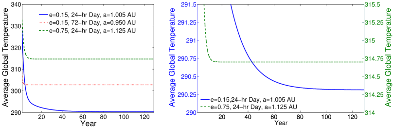
Figure A.— Model relaxation tests. Left: Variations in the average global temperature over the 130-year model evolution for model planets with polar obliquity $\theta_{p}=23.5^{\circ}$ and azimuthal obliquity $\theta_{a}=0^{\circ}$ and a variety of eccentricities, rotation rates, and semimajor axes. The average global temperature is smoothed by a 1-year boxcar filter for the entire 130-year model evolution of a planet. The slowly rotating planet reaches a steady climate state after $\lesssim$10 years, but as shown in the right panel, the planets with 24-hr days require longer model runs to reach a steady climate state. Right: A more detailed plot of the average global temperature for the model planets with rotation rate $\Omega_{p}=\Omega_{\earth}$ highlighting the transition to a steady climate state. The planet with eccentricity $e=0.15$ cools to $T\sim$290.3 K after $\sim$90 years, but the planet with eccentricity $e=0.75$ reaches a steady climate state with $T=314.7$ K after only $\sim$17 years. As before, the global mean temperature is smoothed by a 1-year boxcar filter.

Table 1Model Values for the Surface Heat Capacity $C$

Surface Type	Effective Heat Capacity (erg cm-2 K-1)
Land	$C_{l}$ = 5.25 $\times$ 109
Ocean	$C_{o}$ = 40$C_{l}$
Ice (263 K $<$ T $<$ 273 K)	$C_{i}$ = 9.2$C_{l}$
Ice (T $<$ 263 K)	$C_{i}$ = 2.0$C_{l}$

Table 2Sensitivity Study for a Planet with Eccentricity $e=0.2$

Variation in Model			Outer Edge	Change from
Parameters			of HZ (AU)	Fiducial Model (AU)
Fiducial Model (Earth with $e$ = 0.2)			1.010-1.015	N/A
$\theta_{p}$ = 23.5∘	$\theta_{a}$ = 30∘	Ocean Fraction = 0.7	1.010-1.015	0.000
$\theta_{p}$ = 23.5∘	$\theta_{a}$ = 90∘	Ocean Fraction = 0.7	1.010-1.015	0.000
$\theta_{p}$ = 0∘	$\theta_{a}$ = 0∘	Ocean Fraction = 0.7	1.015-1.020	0.005
$\theta_{p}$ = 15∘	$\theta_{a}$ = 0∘	Ocean Fraction = 0.7	1.010-1.015	0.000
$\theta_{p}$ = 30∘	$\theta_{a}$ = 0∘	Ocean Fraction = 0.7	1.010-1.015	0.000
$\theta_{p}$ = 60∘	$\theta_{a}$ = 0∘	Ocean Fraction = 0.7	1.030-1.035	0.020
$\theta_{p}$ = 90∘	$\theta_{a}$ = 0∘	Ocean Fraction = 0.7	1.050-1.055	0.040
$\theta_{p}$ = 23.5∘	$\theta_{a}$ = 0∘	Ocean Fraction = 0.9	1.010-1.015	0.000
$\theta_{p}$ = 23.5∘	$\theta_{a}$ = 0∘	Ocean Fraction = 0.5	1.010-1.015	0.000
$\theta_{p}$ = 23.5∘	$\theta_{a}$ = 0∘	Ocean Fraction = 0.1	0.990-0.995	-0.020
$\theta_{p}$ = 0∘	$\theta_{a}$ = 0∘	Ocean Fraction = 0.1	0.995-1.000	-0.015
$\theta_{p}$ = 90∘	$\theta_{a}$ = 0∘	Ocean Fraction = 0.1	1.255-1.260	0.245

Table 3Sensitivity Study for a Planet with Eccentricity ${e=0.5}$

Variation in			Outer Edge	Change from
Model Parameters			of HZ (AU)	Fiducial Model (AU)
Fiducial Model (Earth with $e=0.5$)			1.070-1.075	N/A
$\theta_{p}$ = 23.5∘	$\theta_{a}$ = 30∘	Ocean Fraction = 0.7	1.245-1.250	0.175
$\theta_{p}$ = 23.5∘	$\theta_{a}$ = 90∘	Ocean Fraction = 0.7	1.065-1.070	-0.005
$\theta_{p}$ = 0∘	$\theta_{a}$ = 0∘	Ocean Fraction = 0.7	1.070-1.075	0.000
$\theta_{p}$ = 15∘	$\theta_{a}$ = 0∘	Ocean Fraction = 0.7	1.070-1.075	0.000
$\theta_{p}$ = 30∘	$\theta_{a}$ = 0∘	Ocean Fraction = 0.7	1.365-1.370	0.295
$\theta_{p}$ = 60∘	$\theta_{a}$ = 0∘	Ocean Fraction = 0.7	1.765-1.785	0.703
$\theta_{p}$ = 90∘	$\theta_{a}$ = 0∘	Ocean Fraction = 0.7	1.900-1.920	0.838
$\theta_{p}$ = 23.5∘	$\theta_{a}$ = 0∘	Ocean Fraction = 0.9	1.075-1.080	0.005
$\theta_{p}$ = 23.5∘	$\theta_{a}$ = 0∘	Ocean Fraction = 0.3	1.090-1.095	0.020
$\theta_{p}$ = 23.5∘	$\theta_{a}$ = 0∘	Ocean Fraction = 0.1	1.255-1.260	0.185
$\theta_{p}$ = 0∘	$\theta_{a}$ = 0∘	Ocean Fraction = 0.1	1.070-1.075	0.000
$\theta_{p}$ = 90∘	$\theta_{a}$ = 0∘	Ocean Fraction = 0.1	1.415-1.420	0.345

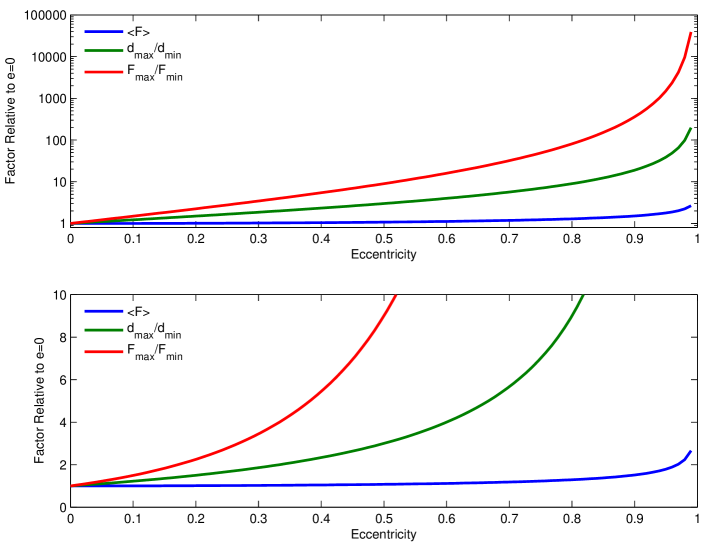
Figure 2.— Comparison of the mean flux (blue) and the ratio of periastron flux to apoastron flux (red) for planets in eccentric orbits to those of planets in circular orbits. The top plot is logarithmic and extends from $e=0$ to $e=1$ while the bottom plot is linear to highlight the change in flux between $e=0$ and $e=0.5$. For reference, the green line shows the distance of the planet at apoastron relative to the distance of the planet at periastron. Although the average flux changes by less than a factor of two even at very high eccentricity, the change in flux over the course of the orbit is several orders of magnitude larger for planets at high eccentricity. Consequently, regions of those planets may be both well below 273 K and well above 373 K during the course of a year. Provided the planets do not freeze over completely during the long winter and enter a snowball state, this raises the question of whether life would be able to withstand such extreme temperature variations.

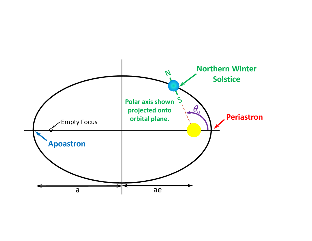
Figure 3.— Top view of a planet in an elliptical orbit with semimajor axis $a$ and eccentricity $e$. As explained in Section 3, the azimuthal obliquity $\theta_{a}$ is zero if periastron is aligned with the projection of the planet’s spin angular momentum vector onto the orbital plane. In that case, northern winter coincides with periastron.

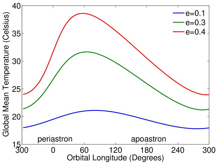
Figure 4.— Our version of Figure 2 of Williams & Pollard (2002). Their model used a test planet with the geography of the Earth while our model used a test planet with a uniform continent distribution but the same 70% ocean fraction as the Earth. The slight differences between their results and ours might be due to the presence of an asymmetric southern continent (Antarctica) in their model but not ours, and other model differences between their three-dimensional GCM and our simpler one-dimensional EBM.

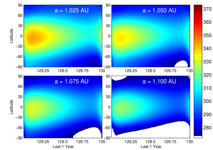
Figure 5.— Temperature as a function of latitude and time of year for a set of planets with $e=0.6$, $\theta_{p}=23.5^{\circ}$, $\theta_{a}=0^{\circ}$, $f_{o}=70\%$ and rotation rate $\Omega_{p}=\Omega_{\earth}$ with a range of semimajor axes. The color indicates temperature as shown in the colorbar. Areas of the planet shown in white are either below 273 K or above 373 K. The planet is completely habitable at 1.025 AU, but the temperature near the south pole drops below freezing during the southern winter at 1.050 AU. The southern ice coverage grows for semimajor axes $>1.075$ AU and is accompanied by northern ice coverage during northern winter at 1.100 AU. Beyond 1.125 AU, the planet is completely frozen.

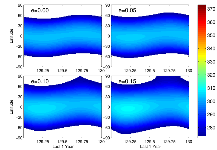
Figure 6.— Temperature as a function of latitude and time of year for a set of planets with $\theta_{p}$ = 23.5^∘, $\theta_{a}$ = 0^∘, $f_{o}=70\%$ and rotation rate $\Omega_{p}=\Omega_{\earth}$. All of the planets are in an orbit with semimajor axis $a=1$ AU, but the eccentricity varies from $e=0$ (top left) to $e=0.15$ (bottom right). At near-zero eccentricity, only the mid-latitudes are habitable, but at high eccentricities, the polar regions receive greater mean isolation over the course of the year and the regional habitability fraction increases. In addition, note that the temperature asymmetry between the northern and southern hemispheres due to the alignment of periastron with northern winter is more pronounced at higher eccentricities because northern winter occurs much closer to the star than southern winter.

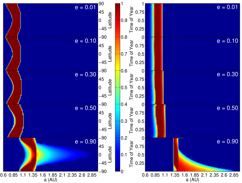
Figure 7.— Left: Temporal habitability fraction (the fraction of a year for which a given latitude band is habitable) for planets with $\theta_{p}=0^{\circ}$, $\theta_{a}=0^{\circ}$, ocean fraction = 70%, and $\Omega_{p}=\Omega_{\earth}$. The eccentricity of each set of planets is indicated and increases downward from $e$ = 0.01 to $e$ = 0.90. Note that the maximum habitable semimajor axis increases for greater eccentricities. Regions shown in red indicate that the region is habitable for the entire year while regions shown in blue indicate that the region is non-habitable for the entire year. Colors between red and blue signify that the region is habitable for part of the year. Right: Regional habitability fraction (the fraction of the surface that is habitable at a given time) for the same planets as in the left panel. Note the increased seasonal dependence at higher eccentricities due to the extreme variations in flux over the orbit. Times shown in red indicate that the entire planet is habitable at that time while times shown in blue indicate that the entire planet is non-habitable at that time. Colors between red and blue signify that a fraction of the planet is habitable at that time.

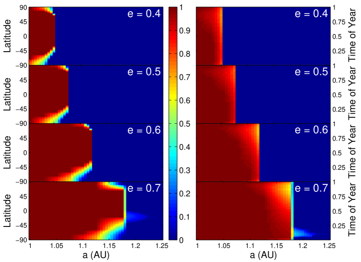
Figure 8.— Same as Figure 7 but for planets with $\theta_{p}=23.5^{\circ}$. Eccentricity increases downward from $e=0.4$ for the top plots to $e=0.7$ for the bottom plots. Left: Temporal habitability fraction as a function of semimajor axis. Right: Regional habitability fraction as a function of semimajor axis. Note that the light shades of blue at $a=1.2$ AU in the plots corresponding to planets with eccentricity $e=0.7$ means that a small fraction of the planet is habitable for a brief period in during southern fall. Comparison with the left panel reveals that the area of the planet that is is transiently habitable during southern fall is near $-30^{\circ}$S, which is near the substellar point at periastron.

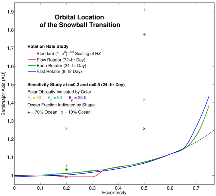
Figure 9.— Effect of rotation rate on the position of the snowball transition. Each line displays the approximate location of the snowball transition for planets with 72-hr days (red), 24-hr days (green), and 8-hr days (blue). For comparison, the symbols mark the position of the snowball transition for several of the model planets with 24-hr days used in the sensitivity study discussed in Section 5.2. The orbital and planetary parameters for those planets are indicated above; for all other model planets ${\theta_{p}=23.5^{\circ}}$, ${\theta_{a}=0^{\circ}}$, and ${f_{o}=0.7}$. The black line shows where the (fixed-atmosphere) outer boundary of the habitable zone would be if it followed the $(1-e^{2})^{-1/4}$ scaling that is sometimes assumed. This scaling has been used by previous studies to estimate the position of the habitable zone, and matches well with our modeled habitable zones for eccentricities ${\lesssim 0.65}$. Planets in more eccentric orbits appear to be habitable at greater semimajor axes than the simple scaling relationship would predict. For instance, the planet with ${\theta_{p}=90^{\circ}}$ and ${f_{o}=0.7}$ is habitable out to 1.90 AU. Rotation rate has little effect on the position of the snowball transition for eccentricities between 0.35 and 0.65, but increasing rotation rate appears to extend the position of the habitable zone for highly eccentric planets. In low eccentricity orbits, the relationship between rotation rate and maximum habitable semimajor axis is not monotonic. The complex relationship may indicate that the semimajor axis of the snowball transition is maximized when the planet rotates slowly enough that sufficient heat is transported to the mid-latitudes to prevent the advance of global permanent ice coverage but quickly enough that a significant amount of heat is retained in the low-latitudes.

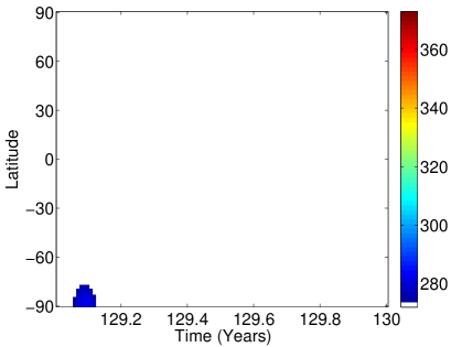
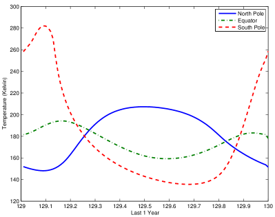
Figure 10.— Temperature profile of a pseudo-Earth with rotation rate $\Omega_{p}=\Omega_{\earth}$, azimuthal obliquity $\theta_{a}=0$, polar obliquity $\theta_{p}=90$, and ocean fraction = 10% in an eccentric orbit with semimajor axis with $a=1.255$ AU and eccentricity $e=0.20$. Left: Habitability map of the planet with colors representing temperature as shown in the color bar. The planet is completely frozen for most of the year, but the southern hemisphere warms to just above 273 K during southern summer at periastron. Right: Temperature variations during the course of the year for the latitude bands at the equator, north pole, and south pole. Although the south pole is the only region of the planet that ever becomes habitable, it also experiences the most extreme temperature variations of any region on the planet.

References

- Adams et al. (2008) Adams, E. R., Seager, S., & Elkins-Tanton, L. 2008, ApJ, 673, 1160
- Agnor et al. (1999) Agnor, C. B., Canup, R. M., & Levison, H. F. 1999, Icarus, 142, 219
- Baglin (2003) Baglin, A. 2003, Advances in Space Research, 31, 345
- Barkstrom et al. (1990) Barkstrom, B. R., Harrison, E. F., & Lee, III, R. B. 1990, EOS Transactions, 71, 279
- Barnes (2007) Barnes, J. W. 2007, PASP, 119, 986
- Barnes et al. (2008) Barnes, R., Raymond, S. N., Jackson, B., & Greenberg, R. 2008, Astrobiology, 8, 557
- Beaulieu et al. (2006) Beaulieu, J.-P., Bennett, D. P., Fouqué, P., Williams, A., Dominik, M., Jorgensen, U. G., Kubas, D., Cassan, A., Coutures, C., Greenhill, J., Hill, K., Menzies, J., Sackett, P. D., Albrow, M., Brillant, S., Caldwell, J. A. R., Calitz, J. J., Cook, K. H., Corrales, E., Desort, M., Dieters, S., Dominis, D., Donatowicz, J., Hoffman, M., Kane, S., Marquette, J.-B., Martin, R., Meintjes, P., Pollard, K., Sahu, K., Vinter, C., Wambsganss, J., Woller, K., Horne, K., Steele, I., Bramich, D. M., Burgdorf, M., Snodgrass, C., Bode, M., Udalski, A., Szymański, M. K., Kubiak, M., Wiȩckowski, T., Pietrzyński, G., Soszyński, I., Szewczyk, O., Wyrzykowski, Ł., Paczyński, B., Abe, F., Bond, I. A., Britton, T. R., Gilmore, A. C., Hearnshaw, J. B., Itow, Y., Kamiya, K., Kilmartin, P. M., Korpela, A. V., Masuda, K., Matsubara, Y., Motomura, M., Muraki, Y., Nakamura, S., Okada, C., Ohnishi, K., Rattenbury, N. J., Sako, T., Sato, S., Sasaki, M., Sekiguchi, T., Sullivan, D. J., Tristram, P. J., Yock, P. C. M., & Yoshioka, T. 2006, Nature, 439, 437
- Bennett et al. (2008) Bennett, D. P., Bond, I. A., Udalski, A., Sumi, T., Abe, F., Fukui, A., Furusawa, K., Hearnshaw, J. B., Holderness, S., Itow, Y., Kamiya, K., Korpela, A. V., Kilmartin, P. M., Lin, W., Ling, C. H., Masuda, K., Matsubara, Y., Miyake, N., Muraki, Y., Nagaya, M., Okumura, T., Ohnishi, K., Perrott, Y. C., Rattenbury, N. J., Sako, T., Saito, T., Sato, S., Skuljan, L., Sullivan, D. J., Sweatman, W. L., Tristram, P. J., Yock, P. C. M., Kubiak, M., Szymański, M. K., Pietrzyński, G., Soszyński, I., Szewczyk, O., Wyrzykowski, Ł., Ulaczyk, K., Batista, V., Beaulieu, J. P., Brillant, S., Cassan, A., Fouqué, P., Kervella, P., Kubas, D., & Marquette, J. B. 2008, ApJ, 684, 663
- Berger et al. (2005) Berger, A., Mélice, J. L., & Loutre, M. F. 2005, Paleoceanography, 20, A264019+
- Berger (1976) Berger, A. L. 1976, A&A, 51, 127
- Berger (1978) —. 1978, Journal of Atmospheric Sciences, 35, 2362
- Borucki & for the Kepler Team (2010) Borucki, W. J. & for the Kepler Team. 2010, ArXiv e-prints
- Borucki et al. (2003) Borucki, W. J., Koch, D., Basri, G., Brown, T., Caldwell, D., Devore, E., Dunham, E., Gautier, T., Geary, J., Gilliland, R., Gould, A., Howell, S., & Jenkins, J. 2003, in ESA Special Publication, Vol. 539, Earths: DARWIN/TPF and the Search for Extrasolar Terrestrial Planets, ed. M. Fridlund, T. Henning, & H. Lacoste, 69–81
- Borucki et al. (2009) Borucki, W. J., Koch, D., Jenkins, J., Sasselov, D., Gilliland, R., Batalha, N., Latham, D. W., Caldwell, D., Basri, G., Brown, T., Christensen-Dalsgaard, J., Cochran, W. D., DeVore, E., Dunham, E., Dupree, A. K., Gautier, T., Geary, J., Gould, A., Howell, S., Kjeldsen, H., Lissauer, J., Marcy, G., Meibom, S., Morrison, D., & Tarter, J. 2009, Science, 325, 709
- Borucki et al. (2007) Borucki, W. J., Koch, D. G., Lissauer, J., Basri, G., Brown, T., Caldwell, D. A., Jenkins, J. M., Caldwell, J. J., Christensen-Dalsgaard, J., Cochran, W. D., Dunham, E. W., Gautier, T. N., Geary, J. C., Latham, D., Sasselov, D., Gilliland, R. L., Howell, S., Monet, D. G., & Batalha, N. 2007, in Astronomical Society of the Pacific Conference Series, Vol. 366, Transiting Extrapolar Planets Workshop, ed. C. Afonso, D. Weldrake, & T. Henning, 309–+
- Bouchy et al. (2009) Bouchy, F., Moutou, C., & Queloz, D. 2009, in CoRoT International Symposium I
- Carpenter et al. (2000) Carpenter, E. J., Lin, S., & Capone, D. G. 2000, Applied and Environmental Microbiology, 66, 4514
- Charbonneau et al. (2009) Charbonneau, D., Berta, Z. K., Irwin, J., Burke, C. J., Nutzman, P., Buchhave, L. A., Lovis, C., Bonfils, X., Latham, D. W., Udry, S., Murray-Clay, R. A., Holman, M. J., Falco, E. E., Winn, J. N., Queloz, D., Pepe, F., Mayor, M., Delfosse, X., & Forveille, T. 2009, Nature, 462, 891
- Crucifix et al. (2006) Crucifix, M., Loutre, M. F., & Berger, A. 2006, Space Science Reviews, 125, 213
- del Genio & Zhou (1996) del Genio, A. D. & Zhou, W. 1996, Icarus, 120, 332
- del Genio et al. (1993) del Genio, A. D., Zhou, W., & Eichler, T. P. 1993, Icarus, 101, 1
- Dole (1964) Dole, S. H. 1964, Habitable planets for man (New York, Blaisdell Pub. Co. [1964] [1st ed.].)
- Farrell (1990) Farrell, B. F. 1990, Journal of Atmospheric Sciences, 47, 2986
- Ford et al. (2008) Ford, E. B., Quinn, S. N., & Veras, D. 2008, ApJ, 678, 1407
- Fressin et al. (2009) Fressin, F., Aigrain, S., Charbonneau, D., Fridlund, M., Guillot, T., Knutson, H., Mazeh, T., Pont, F., Rauer, H., & Torres, G. 2009, in Spitzer Proposal ID #534, 534–+
- Gaudi et al. (2008) Gaudi, B. S., Bennett, D. P., Udalski, A., Gould, A., Christie, G. W., Maoz, D., Dong, S., McCormick, J., Szymański, M. K., Tristram, P. J., Nikolaev, S., Paczyński, B., Kubiak, M., Pietrzyński, G., Soszyński, I., Szewczyk, O., Ulaczyk, K., Wyrzykowski, Ł., DePoy, D. L., Han, C., Kaspi, S., Lee, C., Mallia, F., Natusch, T., Pogge, R. W., Park, B., Abe, F., Bond, I. A., Botzler, C. S., Fukui, A., Hearnshaw, J. B., Itow, Y., Kamiya, K., Korpela, A. V., Kilmartin, P. M., Lin, W., Masuda, K., Matsubara, Y., Motomura, M., Muraki, Y., Nakamura, S., Okumura, T., Ohnishi, K., Rattenbury, N. J., Sako, T., Saito, T., Sato, S., Skuljan, L., Sullivan, D. J., Sumi, T., Sweatman, W. L., Yock, P. C. M., Albrow, M. D., Allan, A., Beaulieu, J., Burgdorf, M. J., Cook, K. H., Coutures, C., Dominik, M., Dieters, S., Fouqué, P., Greenhill, J., Horne, K., Steele, I., Tsapras, Y., Chaboyer, B., Crocker, A., Frank, S., & Macintosh, B. 2008, Science, 319, 927
- Hameury et al. (1998) Hameury, J.-M., Menou, K., Dubus, G., Lasota, J.-P., & Hure, J.-M. 1998, MNRAS, 298, 1048
- Hart (1979) Hart, M. H. 1979, Icarus, 37, 351
- Hartmann (1994) Hartmann, D. L. 1994, Global Physical Climatology (Academic Press, New York), 411
- Heap et al. (2008) Heap, S. R., Lindler, D., & Lyon, R. 2008, in Society of Photo-Optical Instrumentation Engineers (SPIE) Conference Series, Vol. 7010, Society of Photo-Optical Instrumentation Engineers (SPIE) Conference Series
- Held et al. (1981) Held, I. M., Linder, D. I., & Suarez, M. J. 1981, Journal of Atmospheric Sciences, 38, 1911
- Junge et al. (2004) Junge, K., Eicken, H., & Deming, J. 2004, Applied and Environmental Microbiology, 70, 550
- Kalnay et al. (1996) Kalnay, E., Kanamitsu, M., Kistler, R., Collins, W., Deaven, D., Gandin, L., Iredell, M., Saha, S., White, G., Woollen, J., Zhu, Y., Chelliah, M., Ebisuzaki, W., Higgins, W., Janowiak, J., Mo, K. C., Ropelewski, C., Wang, J., Leetmaa, A., Reynolds, R., Jenne, R., & Joselph, D. 1996, Bull. Amer. Meteor. Soc., 77, 437
- Kaltenegger & Fridlund (2005) Kaltenegger, L. & Fridlund, M. 2005, Advances in Space Research, 36, 1114
- Kashefi & Lovley (2003) Kashefi, K. & Lovley, D. 2003, Science, 301, 934
- Kasting et al. (1993) Kasting, J. F., Whitmire, D. P., & Reynolds, R. T. 1993, Icarus, 101, 108
- Kistler et al. (1999) Kistler, R., Kalnay, E., Collins, W., Saha, S., White, G., Woollen, J., Chelliah, M., Ebisuzaki, W., Kanamitsu, M., Kousky, V., van del Dool, H., Jenne, R., & Fiorino, M. 1999, Bull. Amer. Meteor. Soc., 82, 247
- Kokubo & Ida (2007) Kokubo, E. & Ida, S. 2007, ApJ, 671, 2082
- Laskar et al. (1993) Laskar, J., Joutel, F., & Robutel, P. 1993, Nature, 361, 615
- Laskar & Robutel (1993) Laskar, J. & Robutel, P. 1993, Nature, 361, 608
- Leger et al. (2009) Leger, A., Rouan, D., Schneider, J., Alonso, R., Samuel, B., Guenther, E., Deleuil, M., Deeg, H., & Fridlund, M. 2009, A&A, submitted, 287
- Loutre et al. (2004) Loutre, M.-F., Paillard, D., Vimeux, F., & Cortijo, E. 2004, Earth and Planetary Science Letters, 221, 1
- Malhotra & Minton (2008) Malhotra, R. & Minton, D. A. 2008, ApJ, 683, L67
- Marotzke & Botzet (2007) Marotzke, J. & Botzet, M. 2007, Geophys. Res. Lett., 34, 16704
- Milankovic (1941) Milankovic, M. 1941, Kanon der Erdbestrahlung und seine Anwendung auf das Eiszeitenproblem (Belgrade, Mihaila Curcica)
- North (1975) North, G. R. 1975, J. Atmos. Sci., 32, 2033
- Pierrehumbert (2005) Pierrehumbert, R. T. 2005, Journal of Geophysical Research (Atmospheres), 110, 1111
- Quinn et al. (1991) Quinn, T. R., Tremaine, S., & Duncan, M. 1991, AJ, 101, 2287
- Raymond et al. (2004) Raymond, S. N., Quinn, T., & Lunine, J. I. 2004, Icarus, 168, 1
- Rouan et al. (2009) Rouan, D., Leger, A., & J., S. 2009, in CoRoT International Symposium I
- Showman et al. (2009) Showman, A. P., Cho, J. Y.-K., & Menou, K. 2009, ArXiv e-prints
- Spiegel et al. (2008) Spiegel, D. S., Menou, K., & Scharf, C. A. 2008, ApJ, 681, 1609
- Spiegel et al. (2009) —. 2009, ApJ, 691, 596
- Spiegel et al. (2010) Spiegel, D. S., Raymond, S. N., Dressing, C. D., Scharf, C. A., & Mitchell, J. L. 2010, ArXiv e-prints
- Suarez & Held (1979) Suarez, M. J. & Held, I. M. 1979, J . Geophys. Res., 84, 4825
- Takai et al. (2008) Takai, K., Nakamura, K., Toki, T., Tsunogai, U., Masayuki, M., Miyazaki, J., Hirayama, H., Nakagawa, S., Nunoura, T., & Horikoshi, K. 2008, Microbiology, 72, A926
- Udry & Santos (2007) Udry, S. & Santos, N. C. 2007, ARA&A, 45, 397
- Valencia et al. (2006) Valencia, D., O’Connell, R. J., & Sasselov, D. 2006, Icarus, 181, 545
- Valencia et al. (2007) Valencia, D., Sasselov, D. D., & O’Connell, R. J. 2007, ApJ, 665, 1413
- Voigt & Marotzke (2009) Voigt, A. & Marotzke, J. 2009, Clim. Dyn.
- Walker et al. (1981) Walker, J. C. G., Hays, P. B., & Kasting, J. F. 1981, J. Geophys. Res., 86, 9776
- Ward (1974) Ward, W. R. 1974, J. Geophys. Res., 79, 3375
- Ward (1982) —. 1982, Icarus, 50, 444
- Williams & Kasting (1997) Williams, D. M. & Kasting, J. F. 1997, Icarus, 129, 254
- Williams & Pollard (2002) Williams, D. M. & Pollard, D. 2002, International Journal of Astrobiology, 1, 61
- Williams & Pollard (2003) —. 2003, International Journal of Astrobiology, 2, 1