Accounting for risk of non linear portfolios

Abstract

The presence of non linear instruments is responsible for the emergence of non Gaussian features in the price changes distribution of realistic portfolios, even for Normally distributed risk factors. This is especially true for the benchmark Delta Gamma Normal model, which in general exhibits exponentially damped power law tails. We show how the knowledge of the model characteristic function leads to Fourier representations for two standard risk measures, the Value at Risk and the Expected Shortfall, and for their sensitivities with respect to the model parameters. We detail the numerical implementation of our formulae and we emphasizes the reliability and efficiency of our results in comparison with Monte Carlo simulation.

1 Introduction

In the last two decades, the Econophysics community has deeply investigated the empirical features of historical time series emerging in different financial contexts, ranging from high to low frequency data from the stock exchange to the markets in which bonds, FX rates, commodities, energy, futures, options and many other instruments are traded. Numerous empirical evidences have emerged, sometimes confirming results from the financial-econometrics community, or finding new stylized facts and opening new fields of research Mantegna_Stanley:2000 ; Bouchaud_Potters:2003 ; Voit:2001 ; McCauley:2004 . A well known example is given by the observation that the intra-day or daily stochastic dynamics of stock prices significantly deviates from the behaviour predicted by the geometric Brownian motion. This finding dates back to the work of Mandelbrot Mandelbrot:1963 , whose attention was mainly focused in recognizing realizations of stable processes, and to the analysis of Fama Fama:1965 concerning the long tailed nature of the Dow Jones Industrial Average single components. The statistics of returns has been recently rediscussed in different flavours and its modelling has considerably grown. Very heterogeneous models, able to reproduce the degree of asymmetry and the excess of kurtosis of the measured distributions, have been proposed. A non exhaustive list includes approaches developing from specific distributional assumptions, as it is the case of the Lévy flights Mantegna_Stanley:2000 ; Mantegna:1991 ; Mantegna_StanleyPRL:1994 , the Generalized Student-$t$ or Tsallis distributions Bouchaud_Potters:2003 ; BorlandPRL:2002 ; Bormetti_etal:2007 and the exponential one McCauley_Gunaratne:2003 , and it can be extended to more sophisticated models capturing the stochastic nature of the volatility, see Fouque_etal:2000 ; Dragulescu_Yakovenko:2002 ; Perello_etal:2004 ; Bormetti_etal:2008 and references therein, the power law scaling of its autocorrelation function and the leverage effect Bouchaud_Potters:2003 ; Perello_Masoliver:2003 and the multi-fractal properties of historical time series Muzy_etal:2000 ; Pochart_Bouchaud:2002 . The level of complexity grows increasing the dimensionality of the problem. The leptokurtic nature of returns distributions has been shown also for financial indexes, which are linear combinations of plain stocks, such as the Standard & Poor’s 500 Mantegna_Stanley:2000 ; Mantegna:1995 or the NIKKEI Gopikrishnan:1999 . From the point of view of the Central Limit Theorem, this result was not expected: because of the great number of components, the convergence towards the Gaussian regime would be ensured also for heavy tailed stock returns with finite variance. Moving back from the index to the components has proved that the single assets themselves share the same power law scaling, with tail index close to 3 Gopikrishnan2:1999 . Indeed, this fact would be responsible for an ultra slow convergence to Normality for independent stocks; however the existence of strong correlations among assets is a well known evidence which violates the assumptions of the Central Limit Theorem.

In this paper we investigate a completely different mechanism at work, even when the single factors governing the aggregate behaviour are assumed to be Gaussian. We move from the analysis of financial indexes to the case of portfolios where non linear instruments, such as option contracts, induce deviations from Normality, which are no more a consequence of the microscopic dynamics. In the following sections we will review the standard Delta Gamma Normal (DGN) approach to the problem of risk management for non linear portfolios and we will discuss a novel analytical methodology and its efficient numerical implementation. In particular, our aim is to evaluate two standard risk measures, the Value-at-Risk (VaR) and the Expected Shortfall (ES) in the framework of the DGN approximation. For an introduction we refer the reader to the standard financial literature  Jorion:2001 ; Mina:2001 ; Acerbi:2002 . As far as the single asset case is concerned, many different approaches can be adopted. A widely exploited technique in risk analysis, requiring no assumptions on the distribution of the data consists in using past returns realizations to compute risk exposure levels, which are associated to the empirical quantiles of the distribution. Despite its simplicity and generality, such approach suffers from the typical drawbacks related to finite size effects. On the other hand, if an assumption is made on the data distribution, various parametric approaches are available, both in a frequentist and Bayesian framework, often leading to analytical or semi-analytical expressions for VaR and ES Mina:2001 ; Kondor:2001 . Beyond the standard results for Normally distributed asset returns, in Econophysics risk measures have been evaluated with heavy tailed probability density functions (PDF), see for example Bouchaud_Potters:2003 and approaches based on generalized Student-$t$ Bormetti_etal:2007 , Tsallis Mantegna:2004 and Truncated Lévy random variables Bormetti:2010 . Equivalent estimates to those for i.i.d. Student-$t$ variables can also be recovered in a different approach exploiting Bayesian Product Partition Models for Normal independent but not identically distributed returns Bormetti2:2010 . Furthermore, advanced approaches based on the so-called downside risk and applied to the specific case of hedge funds can be found in Lhabitant:2002 ; Perello:2007 . In this paper, we follow an alternative approach based on the generalized Fourier representation of the PDF, already developed in Bormetti:2010 for the single asset case. Fourier techniques for VaR evaluation have been introduced since the work of Rouvinez Rouvinez:1997 , and recently Martin Martin:2009 provided an extension of this framework, obtaining expressions also for the ES and its sensitivities. However, despite being in semi-closed form, they are not straightforwardly suited to numerical evaluation but require a saddle point approximation. On the contrary our analytical formulae can be easily and efficiently evaluated by means of standard trapezoidal integration or Fast Fourier algorithms.

This article is organized as follows. In section 2 we review the portfolio model we consider, outlining the available analytical information (its characteristic function and the corresponding asymptotic tail behaviour of the PDF). In that section we derive the semi-analytical expressions for the VaR, ES, and their sensitivities with respect to the model parameters, which represent the original contribution of this work. In section 3 we compare the numerical results obtained through our expressions with those from the Monte Carlo simulation of synthetic portfolios. Eventually, the relevant conclusions are drawn in section 4.

2 A first step beyond the Normal behaviour

A realistic financial situation usually involves portfolios containing relevant quantities of non linear (options) instruments. A description of these portfolios in terms of a linear composition of risk factors is inadequate, especially when assessing the market risk exposure. An improvement consists in taking a second order expansion of portfolio variations in the risk factors. In particular, when these are assumed to be Normally distributed, one obtains the DGN model. Since this model has become a benchmark framework in the common practice of portfolio risk management, in the present work we do not discuss the limits of applicability of the DGN approximation, which are analyzed in Mina:2001 ; Mina:1999 ; Britten-Jones:1999 .

2.1 The Delta Gamma Normal approach

According to the DGN model, the portfolio price change $V$ over a given time horizon $\Delta t$ is described by the quadratic form

$$V=\theta+\Delta^{\top}X+\frac{1}{2}X^{\top}\Gamma X\ ,$$ (1)

where $X$ is the $N$-dimensional vector of the risk factors which are responsible for the portfolio fluctuations. Here, the variation is defined as $V=W-W_{0}$, where $W_{0}$ denotes the value of the portfolio at the present time $t=t_{0}$, while $W$ is the corresponding value at $t=t_{0}+\Delta t$. The DGN model assumes $X$ to be drawn from a multivariate Gaussian distribution $\mathcal{N}(0,\Sigma)$ with zero mean and covariance matrix $\Sigma$. In equation (1) $\theta\in\mathbb{R}$ and $\Delta\in\mathbb{R}^{N}$ are constants, and so is the real symmetric $N\times N$ matrix $\Gamma$ which accounts for possible non linearities.

By solving the generalized eigenvalue problem

$$CC^{\top}=\Sigma\quad\mathrm{and}\quad C^{\top}\Gamma C=\Lambda\ ,$$ (2)

with $\Lambda=\mathrm{diag}(\lambda_{1},\ldots,\lambda_{N})$, equation (1) can be conveniently rewritten as

$$V=\theta+\sum_{i=1}^{N}\left(\delta_{i}Y_{i}+\frac{\lambda_{i}}{2}Y_{i}^{2}\right)\ ,$$ (3)

where $\delta=C^{\top}\Delta$ and $X=CY$. The $Y_{i}$’s now represent independent standard Gaussian variables, and the correlation structure between the actual risk factors contained in $X$ is now spread across the new $\delta$ and $\lambda$ parameters through relations (2).

Interestingly, the moment generating function of the random variables appearing in equation (3) has been computed in Jaschke:2002 as a Gaussian integral, yielding

$$\mathbb{E}[\mathrm{e}^{\omega(\delta_{i}Y_{i}+(\lambda_{i}Y_{i}^{2})/2)}]=\frac{1}{\sqrt{1-\lambda_{i}\omega}}\exp\left\{-\frac{1}{2}\frac{\delta_{i}^{2}\omega^{2}}{1-\lambda_{i}\omega}\right\}\ ,$$ (4)

$\omega\in\mathbb{R}$, and since this is a holomorph function in the neighbourhood of $0$, the result can be extended to the complex domain. So, the characteristic function $f$ of (3) can be computed:

$$f(\omega)=\mathbb{E}[\mathrm{e}^{\mathrm{i}\omega V}]=\mathrm{e}^{\mathrm{i}\theta\omega}\prod_{i=1}^{N}\frac{1}{\sqrt{1-\mathrm{i}\lambda_{i}\omega}}\exp\left\{-\frac{1}{2}\frac{\delta_{i}^{2}\omega^{2}}{1-\mathrm{i}\lambda_{i}\omega}\right\}\ .$$ (5)

Risk assessment applications typically require a careful estimation of the tails. Even though not required by the VaR and ES evaluation presented in this paper, we devote the last part of the present subsection to review the analytical results for the tails of the PDF of the DGN model, which have been fully characterized by Jaschke et al. in Jaschke:2004 . Indeed, let us suppose that the $\lambda_{i}$ eigenvalues have been ordered in increasing order, and let $n\leq N$ be the number of distinct values. Let $i_{k}$ be the highest index of the $k$-th distinct eigenvalue (so that $\lambda_{i_{1}}<\ldots<\lambda_{i_{n}}$) and let $m_{k}$ be its multiplicity. Then we can define the following useful quantities for $k=1,\cdots,n$

$$\bar{\delta}_{k}^{2}=\sum_{j=i_{k-1}+1}^{i_{k}}\delta_{j}^{2}\quad\mathrm{and}\quad a_{k}^{2}=\frac{\bar{\delta}_{k}^{2}}{\lambda_{i_{k}}^{2}}\ .$$

The left tail behaviour of the PDF $p(V)$ is determined by the sign of the lowest eigenvalue $\lambda^{*}\doteq\lambda_{i_{1}}$. When $\lambda^{*}<0$, the left tail displays an exponentially damped power law decay, whose rate is actually given by $\lambda^{*}$. More precisely, when $V\rightarrow-\infty$, $p(V)$ has the following asymptotic tail behaviour

$$p(V) =c(\delta,\lambda)\ |V|^{\bar{m}}\ \mathrm{e}^{V/\lambda^{*}+a_{1}\sqrt{|2V/\lambda^{*}|}}$$

$$\times\big{(}1+O(1/\sqrt{|V|})\big{)}\ ,$$ (6)

where

$$\bar{m}=\left\{\begin{array}[]{ll}(m_{1}-3)/4&\ \ \ \mathrm{if}\ \ a_{1}\neq 0\\ m_{1}/2-1&\ \ \ \mathrm{if}\ \ a_{1}=0\ .\end{array}\right.$$

When $\lambda^{*}=0$, the left tail is characterized by an asymptotically Gaussian scaling:

$$p(V) =d(\delta,\lambda)\ |V-V_{0}|^{-\frac{1}{2}\sum_{k=2}^{n}m_{k}}\mathrm{e}^{-(V-V_{0})^{2}/(2\bar{\delta}_{1}^{2})}$$

$$\times\big{(}1+O(1/|V-V_{0}|)\big{)}\ ,$$ (7)

where $V_{0}=\theta-\sum_{k=2}^{n}\bar{\delta}_{k}^{2}/(2\lambda_{i_{k}})$. It is worth mentioning that, both in this case and the previous one, the contribution coming from the power law factor may not be negligible when estimating relevant quantiles; moreover, in this context deviations from Gaussianity arise as a consequence of the inclusion of second order terms in the portfolio variation (1), and not of the assumption of a fat tailed distribution for the risk factors.

Lastly, when $\lambda^{*}>0$ the PDF is zero for $V\leq V_{\mathrm{inf}}$, with $V_{\mathrm{inf}}=\theta-\sum_{k=1}^{n}\bar{\delta}_{k}^{2}/(2\lambda_{i_{k}})$, and it decays as a power law in the limit $V\rightarrow V_{\mathrm{inf}}^{+}$:

$$p(V)=k(\delta,\lambda)\ (V-V_{\mathrm{inf}})^{N/2-1}\big{(}1+O(V-V_{\mathrm{inf}})\big{)}~{}.$$ (8)

In equations (6), (7), (8), $c(\delta,\lambda)=c(\delta_{i=1,\ldots,N},\lambda_{i=1,\ldots,N})$, $d(\delta,\lambda)$ and $k(\delta,\lambda)$ are constants depending on the set of parameters in use.

As far as risk estimation is concerned, the left tail decay is what we are interested in; however, previous considerations apply to the right tail in an antithetic way depending on the sign of the highest eigenvalue $\lambda_{i_{n}}$. When $\lambda_{i_{n}}>0$ ($\lambda_{i_{n}}=0$) the right tail is exponential (Gaussian) in the limit $V\to+\infty$; otherwise, the support of $p(V)$ is limited from the right and for $V\to V_{\mathrm{sup}}^{-}$ it scales as a power law with exponent $N/2-1$ and $V_{\mathrm{sup}}=\theta-\sum_{k=1}^{n}\bar{\delta}_{k}^{2}/(2\lambda_{i_{k}})$.

The central moments of the distribution of $V$ can be also explicitly derived, and the first four of them read Jaschke:2002 ; Mina:1999 ; Britten-Jones:1999 :

$$\mu_{1} =\theta+\frac{1}{2}\mathrm{tr}[\Gamma\Sigma]$$

$$\mu_{2} =\Delta^{\top}\Sigma\Delta+\frac{1}{2}\mathrm{tr}[(\Gamma\Sigma)^{2}]$$

$$\mu_{3} =3\Delta^{\top}\Sigma\Gamma\Sigma\Delta+\mathrm{tr}[(\Gamma\Sigma)^{3}]$$

$$\mu_{4} =12\Delta^{\top}\Sigma(\Gamma\Sigma)^{2}\Delta+3\ \mathrm{tr}[(\Gamma\Sigma)^{4}]+3\mu_{2}^{2}\ .$$

From these relations explicit expressions for the skewness $\zeta=\mu_{3}/\mu_{2}^{3/2}$ and the kurtosis $\kappa=\mu_{4}/\mu_{2}^{2}-3$ can be derived, and one can easily check that whenever $\Gamma=0$ we have $\zeta=0$ and $\kappa=0$. This is coherent with the fact that equations (1) and (3) define a Gaussian portfolio model when their quadratic terms are set to zero, i.e. when $\Gamma=0$. From this point of view, the possible presence of asymmetries or non Gaussian tails in the PDF of the DGN model stems from the non linear terms in (1) and (3).

2.2 Formulae for risk estimation

The risky nature of a portfolio can be accounted for via the well-known VaR estimator, which gives the potential loss (negative variation) over the time horizon $\Delta t$ that could be exceeded with probability equal to the significance level $\mathcal{P}^{*}$. However the VaR is known to suffer from two main drawbacks, the lack of subadditivity and of information about the average potential loss when the VaR threshold is exceeded. Both of them are overcome by introducing an alternative and coherent measure Acerbi:2002 known as the ES.

To obtain semi-analytical expressions for the risk measures, the steps followed in Bormetti:2010 are substantially replied. We fix a significance level $\mathcal{P}^{*}\in(0,1)$ and we define the VaR $\Delta^{*}$ as

$$\mathcal{P}^{*} =\int_{-W_{0}}^{-\Delta^{*}}\mathrm{d}V\ p(V)$$

$$=\int_{-\infty}^{-\Delta^{*}}\mathrm{d}V~{}p(V)-\int_{-\infty}^{-W_{0}}\mathrm{d}V~{}p(V)\ .$$ (9)

In this expression $-W_{0}$ represents the maximum possible loss over $\Delta t$. Compared to Bormetti:2010 , this framework involves portfolio variations instead of logarithmic returns and this leads to the finite lower bound of integration in the first line of equation (9). Since we are modelling the risk factors as Gaussian random variables, $p(V)$ could have unbounded support; nevertheless, under the assumption that the DGN $p(V)$ is a good approximation to the true (unknown) PDF, we expect $-W_{0}$ to be on the far left tail of $p(V)$ and the second term of equation (9) to be negligible . For this reason, in the following expressions, we always imply the limit $-W_{0}\to-\infty$.

We now represent $p(V)$ in terms of its generalized Fourier transform

$$p(V)=\frac{1}{2\pi}\int_{-\infty+\mathrm{i}\nu}^{+\infty+\mathrm{i}\nu}\mathrm{d}\phi~{}f(\phi)~{}\mathrm{e}^{-\mathrm{i}\phi V}\ ,$$ (10)

where the axis of integration in the complex plane has to be chosen parallel to the real axis with imaginary part $\nu$ belonging to the strip of regularity $(\nu_{-},\nu_{+})$ of $f$ Lewis:2001 ; Lipton:2001 . The boundaries of the strip of regularity are determined by the singular points of $f$ closest to the origin. If any, singularities must be purely imaginary, and, for the present case, a quick analysis shows that they are equal to $\{-\mathrm{i}/\lambda_{i_{k}},\ k=1,\dots,n\}$. Using the expression (10) and switching the integration order, equation (9) becomes

$$\mathcal{P}^{*}=\frac{1}{2\pi}\int_{-\infty+\mathrm{i}\nu}^{+\infty+\mathrm{i}\nu}\mathrm{d}\phi~{}f(\phi)\left(\int_{-\infty}^{-\Delta^{*}}\mathrm{d}V\mathrm{e}^{-\mathrm{i}\phi V}\right)$$

and the convergence of the innermost integral is guaranteed if we restrict $\nu\in(0,\nu^{+})$. With this choice, the previous expression readily reduces to

$$\mathcal{P}^{*} =\frac{\mathrm{i}}{2\pi}\int_{-\infty+\mathrm{i}\nu}^{+\infty+\mathrm{i}\nu}\mathrm{d}\phi\ \frac{f(\phi)}{\phi}\ \mathrm{e}^{-\mathrm{i}\phi\Delta^{*}}$$

$$=\frac{\mathrm{e}^{-\nu\Delta^{*}}}{\pi}\mathrm{Re}\left[\int_{0}^{+\infty}\mathrm{d}\omega\ \frac{f(\omega+\mathrm{i}\nu)}{\nu-\mathrm{i}\omega}\ \mathrm{e}^{\mathrm{i}\omega\Delta^{*}}\right]\ ,$$ (11)

where $\phi=\omega+\mathrm{i}\nu$. From the previous discussion, we can determine the value of $\nu^{+}$ depending on that of $\lambda^{*}$:

• when $\lambda^{*}<0$, then $\nu_{+}=|1/\lambda^{*}|$;

• when $\lambda^{*}\geq 0$, then $\nu_{+}=+\infty$.

To evaluate the ES the considerations already exposed for VaR evaluation still apply. Starting from its definition and using again equation (10), we can write

$$E^{*}(\mathcal{P}^{*}) =-\frac{1}{\mathcal{P}^{*}}\int_{-\infty}^{-\Delta^{*}}\mathrm{d}V\ V\ p(V)$$

$$=-\frac{1}{2\pi\mathcal{P}^{*}}\int_{-\infty+\mathrm{i}\nu}^{+\infty+\mathrm{i}\nu}\mathrm{d}\phi\ f(\phi)\left[\frac{1}{\phi^{2}}-\frac{\mathrm{i}\Delta^{*}}{\phi}\right]\ \mathrm{e}^{\mathrm{i}\phi\Delta^{*}}$$

$$=-\frac{\mathrm{e}^{-\nu\Delta^{*}}}{\pi\mathcal{P}^{*}}\mathrm{Re}\left[\int_{0}^{+\infty}\mathrm{d}\omega\ \frac{f(\omega+\mathrm{i}\nu)}{(\omega+\mathrm{i}\nu)^{2}}\ \mathrm{e}^{\mathrm{i}\omega\Delta^{*}}\right]$$

$$+\frac{\mathrm{e}^{-\nu\Delta^{*}}}{\pi\mathcal{P}^{*}}\Delta^{*}\mathrm{Re}\left[\int_{0}^{+\infty}\mathrm{d}\omega\ \frac{f(\omega+\mathrm{i}\nu)}{\nu-\mathrm{i}\omega}\ \mathrm{e}^{\mathrm{i}\omega\Delta^{*}}\right]~{},$$

and, recalling the representation (11) of $\mathcal{P}^{*}$, the last expression can be simplified in

$$E^{*}(\mathcal{P}^{*})=\Delta^{*}-\frac{\mathrm{e}^{-\nu\Delta^{*}}}{\pi\mathcal{P}^{*}}\mathrm{Re}\left[\int_{0}^{+\infty}\mathrm{d}\omega\ \frac{f(\omega+\mathrm{i}\nu)}{(\omega+\mathrm{i}\nu)^{2}}\ \mathrm{e}^{\mathrm{i}\omega\Delta^{*}}\right]~{}.$$ (12)

2.3 Sensitivities

We are not only interested in estimating VaR and ES, but also in their sensitivity with respect to the parameters of the DGN model. For a portfolio which is a linear composition of risk factors, $\Delta^{*}$ and $E^{*}$ are 1-homogeneous functions Martin:2009 ; Major:2004 . Indeed, when $\Gamma=0$, we have $\Delta=\delta$ and, posing $\theta=0$ for simplicity, the portfolio VaR reduces to the well known expression

$$\Delta^{*}=-\sqrt{\delta^{T}\Sigma\delta}~{}\sqrt{2}~{}\mathrm{erf}^{-1}(2\mathcal{P}^{*}-1)~{},$$

where $\mathrm{erf}^{-1}$ is the inverse of the error function. The first derivatives of VaR read

$$\frac{\partial\Delta^{*}}{\partial\delta_{k}}=-\frac{\left(\Sigma\delta\right)_{k}}{\sqrt{\delta^{T}\Sigma\delta}}~{}\sqrt{2}~{}\mathrm{erf}^{-1}(2\mathcal{P}^{*}-1)~{},$$

and the homogeneity condition is readily verified

$$\Delta^{*}=\sum_{k=1}^{N}\delta_{k}\frac{\partial\Delta^{*}}{\partial\delta_{k}}~{}.$$

It can be shown that an analogous relation holds for the $E^{*}$. The main consequence is that for linear portfolios, the knowledge of the first derivatives allows, just by itself, for a complete reconstruction of the risk measures. Thus, risk measures response with respect to shocks in the $\delta_{k}$ weights defining the portfolio composition can be fully characterized with no need of computing higher order derivatives.

On the other hand, in this work we consider the effects due to the presence of non linear instruments; in this scenario, a complete description of the market risk exposure would require the knowledge of higher order derivatives. Nevertheless, the first order ones still provide crucial information about the sensitivity of risk measures when shocking the portfolio weights. For this reason, here we report the expressions of the first order derivatives only, reminding the reader that higher order terms can be computed going back through the same passages.

Equation (11) is now differentiated with respect to the generic parameter that, for the sake of tidiness, we address as $\beta$

$$\{\beta\}=(\theta,\delta_{i},\lambda_{i})\ \ \ i=1,\ldots,N\ .$$

Since we aim at evaluating the response of the risk measures with respect to shocks to the portfolio parameters while keeping $\mathcal{P}^{*}$ fixed, we obtain

$$0=\frac{\partial\mathcal{P}^{*}}{\partial\beta}=\frac{\mathrm{e}^{-\nu\Delta^{*}}}{\pi} \mathrm{Re}\left[\int_{0}^{+\infty}\frac{\mathrm{d}\omega}{\nu-\mathrm{i}\omega}\right.\left(\frac{\partial f(\omega+\mathrm{i}\nu)}{\partial\beta}\right.$$

$$\left.\left.+(\mathrm{i}\omega-\nu)f(\omega+\mathrm{i}\nu)\frac{\partial\Delta^{*}}{\partial\beta}\right)\right].$$

Exploiting the previous equality, and recalling equation (10), the VaR sensitivities read

$$\frac{\partial\Delta^{*}}{\partial\beta} =\frac{\mathrm{Re}\left[\int_{0}^{+\infty}\frac{\mathrm{d}\omega}{\nu-\mathrm{i}\omega}\frac{\partial f(\omega+\mathrm{i}\nu)}{\partial\beta}\ \mathrm{e}^{\mathrm{i}\omega\Delta^{*}}\right]}{\mathrm{Re}\left[\int_{0}^{+\infty}\mathrm{d}\omega\ f(\omega+\mathrm{i}\nu)\ \mathrm{e}^{\mathrm{i}\omega\Delta^{*}}\right]}$$ (13)

$$=\frac{\mathrm{e}^{-\nu\Delta^{*}}}{\pi p(-\Delta^{*})}\mathrm{Re}\left[\int_{0}^{+\infty}\frac{\mathrm{d}\omega}{\nu-\mathrm{i}\omega}\frac{\partial f(\omega+\mathrm{i}\nu)}{\partial\beta}\ \mathrm{e}^{\mathrm{i}\omega\Delta^{*}}\right]~{}.$$

Finally, using again (11), differentiation of equation (12) gives us the following Fourier representation of the ES sensitivities

$$\frac{\partial E^{*}(\mathcal{P}^{*})}{\partial\beta} =\frac{\partial\Delta^{*}}{\partial\beta}\left\{1-\frac{\mathrm{e}^{-\nu\Delta^{*}}}{\pi\mathcal{P}^{*}}\right.$$

$$\left.\times~{}\mathrm{Re}\left[\int_{0}^{+\infty}\mathrm{d}\omega\ \frac{f(\omega+\mathrm{i}\nu)}{\nu-\mathrm{i}\omega}\ \mathrm{e}^{\mathrm{i}\omega\Delta^{*}}\right]\right\}$$

$$-\frac{\mathrm{e}^{-\nu\Delta^{*}}}{\pi\mathcal{P}^{*}}\mathrm{Re}\left[\int_{0}^{+\infty}\frac{\mathrm{d}\omega}{(\omega+\mathrm{i}\nu)^{2}}\frac{\partial f(\omega+\mathrm{i}\nu)}{\partial\beta}\ \mathrm{e}^{\mathrm{i}\omega\Delta^{*}}\right]$$

$$= -\frac{\mathrm{e}^{-\nu\Delta^{*}}}{\pi\mathcal{P}^{*}}\mathrm{Re}\left[\int_{0}^{+\infty}\frac{\mathrm{d}\omega}{(\omega+\mathrm{i}\nu)^{2}}\frac{\partial f(\omega+\mathrm{i}\nu)}{\partial\beta}\ \mathrm{e}^{\mathrm{i}\omega\Delta^{*}}\right]~{},$$ (14)

where the final equality holds because the expression in the curly brackets vanishes. Finally we compute the derivatives of the characteristic function appearing in (13) and (14). Using equation (5) we obtain

$$\frac{\partial f(\phi)}{\partial\theta} =\mathrm{i}\phi f(\phi)\ ,$$

$$\frac{\partial f(\phi)}{\partial\delta_{i}} =-\frac{\delta_{i}\phi^{2}}{1-\mathrm{i}\lambda_{i}\phi}~{}f(\phi)\ ,$$

$$\frac{\partial f(\phi)}{\partial\lambda_{i}} =\frac{\mathrm{i}\phi}{2(1-\mathrm{i}\lambda_{i}\phi)}\left[1-\frac{\delta_{i}^{2}\phi^{2}}{1-\mathrm{i}\lambda_{i}\phi}\right]f(\phi)\ .$$ (15)

Incidentally, we notice that all the previous relations, valid for the DGN model, are linear in $f$ and thus equations (13) and (14) share a similar structure with equations (11) and (12).

3 Numerical results

In this section we detail the numerical results of our Fourier approach, computing $\Delta^{*}$, $E^{*}$ and the sensitivities for synthetic portfolios corresponding to the possible cases depending on the value of the smallest eigenvalue $\lambda^{*}$. We check the semi-analytical estimates with the ones obtained by Monte Carlo simulation of the portfolio values. Below, a brief summary of the numerical setup for both the semi-analytical approach, proposed here, and the standard historical simulation one is given.

We do not address the problem of estimating the covariance matrix $\Sigma$ from real portfolio data. Nevertheless, it is worth noticing that the usual parametric Maximum Likelihood estimators of dispersion perform reasonably well in the limit of an infinite number of observations for the risk factors. When the length of the time series $T$ is larger than the number of risk factors $N$, it is also possible to exploit filtering procedures Mantegna:1999 ; Tumminello:2007 , such as hierarchical clustering, to extract the relevant information from correlation matrices, retaining only the statistically significant correlations. These techniques, besides reducing the dimensionality of the problem, can give crucial information for decision processes such as portfolio allocation. Under the thermodynamical limit of $T,N\rightarrow+\infty$, with $T/N$ fixed, the random matrix theory has also proved to be a useful tool to better understand the statistical structure of empirical correlation matrices Laloux:1998 ; Plerou:1999 . On the other hand, when the sample is small, especially when $T$ is smaller than $N$, which is common for large portfolios, the error affecting the Maximum Likelihood estimators is large. In this situations, it is possible to resort to better performing estimators, such as, for instance, the Ledoit and Wolf shrinkage estimator of dispersion Ledoit:2003 ; Meucci:2005 which is a weighted average of the sample covariance $\hat{\Sigma}$ and a target diagonal matrix $\hat{C}$

$$\hat{\Sigma}^{S}=(1-\alpha)\hat{\Sigma}+\alpha\hat{C}\ ,$$

where $\hat{C}=(1/m)\sum_{k=1}^{m}\hat{\eta_{k}}\mathbb{I}$, $\hat{\eta}_{k}$ are the sample estimations of the eigenvalues of $\Sigma$ and $\alpha$ is the optimal shrinkage weight depending on $\hat{\Sigma}$, $\hat{C}$ and $X_{t=1,\dots,T}$.

3.1 Numerical setup

Fourier inversion. The complex integrals involved by our expressions for risk measures and sensitivities are evaluated by means of trapezoidal integration; this requires to split explicitly the real part of the integrand, being an even function of $\omega$, in the two terms proportional to the sine and cosine functions. For instance, evaluation of $\mathcal{P}^{*}$, equation (11), reduces to compute the following two real Fourier integrals

$$\mathcal{P}^{*}=\frac{\mathrm{e}^{-\nu\Delta^{*}}}{\pi} \left\{\int_{0}^{+\infty}\mathrm{Re}\left[\frac{f(\omega+\mathrm{i}\nu)}{\nu-\mathrm{i}\omega}\right]\cos(\omega\Delta^{*})\right.$$

$$-\left.\int_{0}^{+\infty}\mathrm{Im}\left[\frac{f(\omega+\mathrm{i}\nu)}{\nu-\mathrm{i}\omega}\right]\sin(\omega\Delta^{*})\right\}.$$

Each one is solved by means of standard adaptive routines ; similar decompositions apply to the other quantities of interest.
Historical simulation. A sample of $T_{MC}$ realizations of the risk factors $X\sim N(0,\Sigma)$ is drawn and, correspondingly, the time series of the portfolio variations $V_{t=1,\dots,T_{MC}}$ is computed. If $\tilde{V}_{t}$ are the entries of $V_{t}$ sorted in ascending order, and assuming $t^{*}=T_{MC}\times\mathcal{P}^{*}$ to be integer, the historical VaR at the significance level $\mathcal{P}^{*}$ is defined as 

$$\Delta_{\mathrm{H}}^{*}=-\tilde{V}_{t^{*}}~{}.$$ (16)

The ES is obtained as the average on the left tail of the empirical distribution

$$E_{\mathrm{H}}^{*}=-\frac{1}{t^{*}}\sum_{t=1}^{t^{*}}\tilde{V}_{t}~{}.$$ (17)

Confidence intervals for VaR are obtained from a basic result of order statistics. Let us consider the sample of $T_{MC}$ i.i.d. deviates $V_{i}$ and indicate with $Q_{p}$ the $p$-th percentile of their distribution; then, the probability of $Q_{p}$ being enclosed in $(\tilde{V}_{t^{-}},\tilde{V}_{t^{+}})$ is given by the following sum of binomial probabilities David:2003

$$P(\tilde{V}_{t^{-}}<Q_{p}<\tilde{V}_{t^{+}})=\sum_{k=t^{-}}^{t^{+}-1}\binom{T_{MC}}{k}p^{k}(1-p)^{T_{MC}-k}~{}.$$ (18)

To find the confidence interval associated to $\Delta^{*}_{\mathrm{H}}$ for a given Confidence Level (CL), we find indices $t^{\mp}$ satisfying

$$P(\tilde{V}_{t^{-}+1}<Q_{\mathcal{P}^{*}}<\tilde{V}_{t^{+}})\leq CL\leq P(\tilde{V}_{t^{-}}<Q_{\mathcal{P}^{*}}<\tilde{V}_{t^{+}})$$

where $Q_{\mathcal{P}^{*}}=-\Delta^{*}$ and the choice between possible different pairs $(t^{-},t^{+})$ satisfying the previous inequality is made requiring the confidence interval to be as symmetric as possible around $\Delta^{*}_{\mathrm{H}}$. With these positions, Historical VaR is estimated by

$$(\Delta^{*}_{\mathrm{H}})^{+\delta^{+}}_{-\delta^{-}}~{},\quad\left\{\begin{aligned} \delta^{+}&\doteq-\tilde{V}_{t^{-}}-\Delta^{*}_{\mathrm{H}}\\ \delta^{-}&\doteq\Delta^{*}_{\mathrm{H}}+\tilde{V}_{t^{+}}\end{aligned}\right.$$ (19)

with confidence level $CL$.

Since $E^{*}$ is a monotonously increasing function of $\Delta^{*}$, a lower and upper bound for ES are easily obtained by evaluating the average in equation (17) for $t^{*}=t^{-}$ and $t^{*}=t^{+}$ respectively. At the same CL as above, we estimate

$$(E^{*}_{\mathrm{H}})^{+e^{+}}_{-e^{-}}~{},\quad\left\{\begin{aligned} e^{+}&\doteq-\left(\frac{1}{t^{-}}\sum_{k=1}^{t^{-}}\tilde{V}_{k}\right)-E^{*}_{\mathrm{H}}\\ e^{-}&\doteq E^{*}_{\mathrm{H}}+\left(\frac{1}{t^{+}}\sum_{k=1}^{t^{+}}\tilde{V}_{k}\right)\end{aligned}\right.~{}.$$ (20)

The sensitivities of $\Delta^{*}_{\mathrm{H}}$ are evaluated by approximating its derivatives with respect to the remapped parameters of equation (3), with the finite difference formula

$$\left(\partial_{\beta}\Delta^{*}\right)_{\mathrm{H}}\doteq\left(\frac{\partial\Delta^{*}}{\partial\beta}\right)_{\mathrm{H}}=\frac{\Delta^{*}_{\mathrm{H}}(\beta+\Delta\beta)-\Delta^{*}_{\mathrm{H}}(\beta-\Delta\beta)}{2\Delta\beta}$$ (21)

where $\Delta^{*}_{\mathrm{H}}(\beta\pm\Delta\beta)$ denotes the historical estimates for the VaR obtained simulating the DGN portfolio after giving a positive/negative shock to the parameter $\beta$ while keeping fixed all the others. The error affecting $\left(\partial_{\beta}\Delta^{*}\right)_{\mathrm{H}}$ is obtained by linear propagation of the Monte Carlo errors on $\Delta^{*}_{\mathrm{H}}(\beta\pm\Delta\beta)$ through equation (21). An analogous procedure is applied to estimate $\left(\partial_{\beta}E^{*}\right)_{\mathrm{H}}$ and its confidence interval.

The results discussed in the following sections have been obtained simulating $T_{MC}=10^{7}$ synthetic portfolio scenarios for $N=15$ risk factors; for simplicity, we simulated the remapped factors $Y\sim N(0,\mathbb{I})$ and the values $V_{t}$ were constructed from equation (3) after arbitrarily fixing $\theta$, $\delta$ and $\lambda$. Attention has to be paid here to freeze the values of $Y_{t}$, so that re-evaluation of the portfolio with shocked parameters is always carried out based on the same sample. More details about efficient algorithms to generate the scenarios under a quadratic approximation of the portfolio losses can be found in Glasserman:2002 . The semi-analytical curves have been obtained by Fourier inversion of equations (11), (12), (13) and (14), the characteristic function and its derivatives as given by (5) and (15). Given a grid of $\Delta^{*}$ values, the corresponding $\mathcal{P}^{*}$, $E^{*}$, $\partial_{\beta}\Delta^{*}$ and $\partial_{\beta}E^{*}$ are computed and compared with those from the historical simulation. If one is interested in $\Delta^{*}$ corresponding to a precise spot value of $\mathcal{P}^{*}$, inversion of equation (11) has to be nested in a root finding procedure. Alternatively, the grid of $\Delta^{*}$ can be tuned in such a way to obtain $\mathcal{P}^{*}$ values close enough to the required one.

3.2 The lowest eigenvalue is negative

In order to discuss the case $\lambda^{*}<0$, we fix the DGN parameters as follows: $\theta=0$, $\delta_{i=1,\cdots,15}=1$, $\lambda^{*}=\lambda_{i=1,\cdots,5}=-2$, $\lambda_{i=6,\cdots,9}=1$ and $\lambda_{i=10,\cdots,15}=2$ (CASE 1).

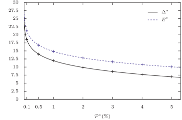
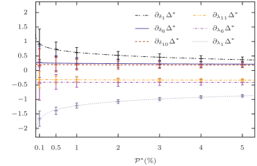
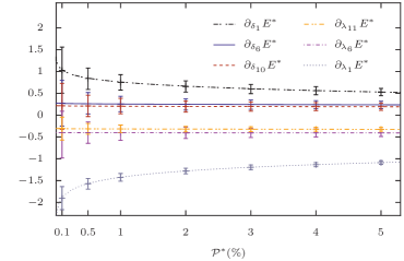
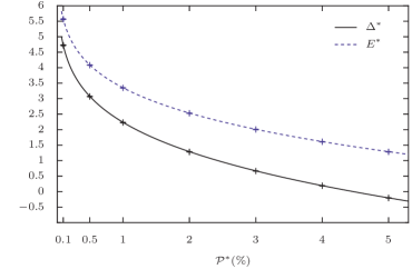
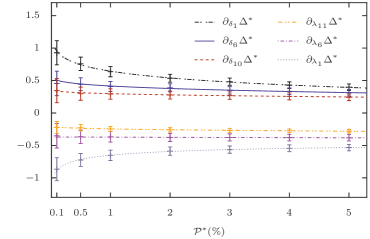
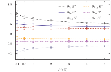
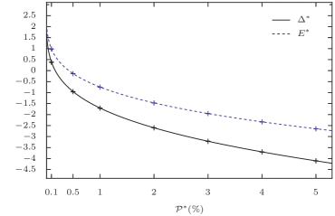
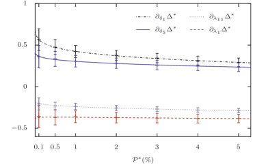
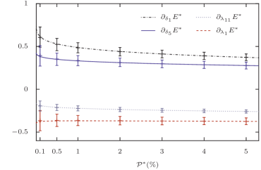
The correspondence $\mathcal{P}^{*}$-VaR and $\mathcal{P}^{*}$-ES as obtained from equations (11),(12) is shown in Figure 1. As expected from their definitions, $E^{*}$ estimates are always larger than $\Delta^{*}$, the shift vanishing in the limit of $\mathcal{P}^{*}$ approaching $0$. The sensitivities for this set of parameters are illustrated in Figure 2 and Figure 3. With the exception of $\beta=\theta$, the derivatives of $f(\phi)$ always depend on the pair $(\delta_{i},\lambda_{i})$; for this reason the only cases we need to consider are $\beta=\theta,\delta_{1,6,10},\lambda_{1,6,10}$. The sensitivities with respect to the central value $\theta$ are identically equal to $-1$; this result can be verified directly from equations (13),(14) after substitution of $\partial_{\theta}f(\phi)$ and reminding the definition of $\mathcal{P}^{*}$ and $p(\Delta^{*})$, and the corresponding curves are not shown for the sake of clarity.

All the curves are superimposed to the points obtained through historical simulation for the interesting values of $\mathcal{P}^{*}=0.001,0.005,0.01,0.02,0.03,0.04,0.05$, along with the corresponding error bars for $CL=98\%$; central points and error bounds correspond to the definitions (19), (20) for $\Delta^{*}$ and $E^{*}$ and to their extensions for the sensitivities. The latter exhibit larger uncertainty, due to the propagation of the statistical error, which is magnified by the finite difference formula (21) by a factor of order $\mathcal{O}(1/\Delta\beta)$. It is also clear how this uncertainty increases for smaller $\mathcal{P}^{*}$, due to the decreasing size of the sample on the left tail of the distribution of the generated values $V_{t}$. On the whole, the full agreement with the Monte Carlo outcomes proves the effectiveness of our analytical results and the reliability of their numerical implementation.

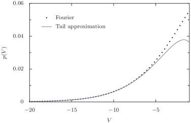
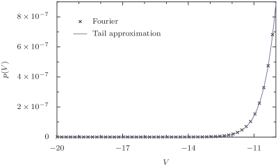
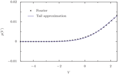
As discussed in section 2, in this case the distribution function $p(V)$ has both left and right exponential tails. This scaling is confirmed by Figure 4, where the left tail of the PDF, reconstructed by Fourier inversion of equation (10), is fitted by its asymptotic approximation (6).

Figure 1: (Color online) CASE 1 ($\lambda^{*}<0$): VaR and ES. The semi-analytical curves are compared to the points obtained via historical simulation for the values of $\mathcal{P}^{*}$ usually considered in practice.

Figure 2: (Color online) CASE 1: Value at Risk sensitivities.

Figure 3: (Color online) CASE 1: Expected Shortfall sensitivities.

Figure 4: (Color online) CASE 1: left tail of the PDF fitted by its analytical approximation corresponding to exponential decay.

3.3 The lowest eigenvalue is zero

The case $\lambda^{*}=0$ is discussed here for the set of parameters: $\theta=0$, $\delta_{i=1,\cdots,15}=1$, $\lambda^{*}=\lambda_{i=1,\cdots,5}=0$, $\lambda_{i=6,\cdots,9}=1$ and $\lambda_{i=10,\cdots,15}=2$. Figure 5-7 show the same curves described above, again exhibiting full statistical agreement with the Monte Carlo simulation. Previous considerations about the statistical errors still apply and the only significant difference is the shape of the PDF in Figure 8, showing a Gaussian decay of the left tail, as expected from the asymptotic expression (7).

Figure 5: (Color online) CASE 2 ($\lambda^{*}=0$): Value at Risk and Expected Shortfall.

Figure 6: (Color online) CASE 2: Value at Risk sensitivities.

Figure 7: (Color online) CASE 2: Expected Shortfall sensitivities.

Figure 8: (Color online) CASE 2: For $\lambda^{*}=0$ the left tail of $p(V)$ exhibits a Gaussian decay as expected from (7).

3.4 The lowest eigenvalue is positive

The last case we consider corresponds to the choices: $\theta=0$, $\delta_{i=1,\cdots,15}=1$, $\lambda^{*}=\lambda_{i=1,\cdots,4}=1$ and $\lambda_{i=5,\cdots,15}=2$ (CASE 3). Since $\lambda^{*}>0$, the PDF of $V$ is limited from the left, see Figure 12; its support is $[V_{\mathrm{inf}},+\infty)$ with $V_{\mathrm{inf}}=\theta-\sum_{k=1}^{n}\frac{\bar{\delta^{2}_{k}}}{2\lambda_{i_{k}}}=-4.75$, and the left tail approaches $0$ with power law scaling $(V-V_{\mathrm{inf}})^{N/2-1}$, see equation (8). As a consequence of the truncation near the origin of the $V$ axis, $\Delta^{*}$ and $E^{*}$ are negative for a quite large interval of $\mathcal{P}^{*}$ of interest, as illustrated in Figure 9.

For this set of parameters the unique $(\delta,\lambda)$ pairs to be considered are only $(\delta_{1},\lambda_{1})$ and $(\delta_{1},\lambda_{5})$, corresponding to the sensitivities reported in Figures 10, 11.

Figure 9: (Color online) CASE 3 ($\lambda^{*}>0$): Value at Risk and Expected Shortfall. The truncation of the PDF near the origin is responsible for the negative values for $\Delta^{*}$ and $E^{*}$ over a wide interval of $\mathcal{P}^{*}$, see the main text.

Figure 10: (Color online) CASE 3: Value at Risk sensitivities.

Figure 11: (Color online) CASE 3: Expected Shortfall sensitivities.

Figure 12: (Color online) CASE 3: The PDF is limited from the left, decaying as a power law of exponent $N/2-1=6.5$.

4 Conclusions

In this paper, we addressed the problem of the evaluation of market risk exposure for non linear portfolios, when price changes are approximated according to the Delta Gamma Normal model. Exploiting the generalized Fourier representation of the probability density function for the model, semi-closed form expressions for the Value at Risk and the Expected Shortfall were derived. Similarly analogous expressions in terms of a single Fourier integral were obtained for their first order derivatives; thus our approach turns out to be especially useful, since these quantities are of major practical relevance for the purposes of asset allocations and market risk hedging, giving crucial information about the sensitivity of the portfolio with respect to its risky components. It is worth mentioning that our approach could be readily extended to compute higher order derivatives. All of our formulae lend themselves to efficient numerical evaluation; they have been tested by simulating synthetic portfolio scenarios via Monte Carlo. This comparison, while confirming the reliability of our expressions with a full statistical agreement, highlights their potential in practical applications, since full Monte Carlo evaluation would require very large samples to obtain accurate risk estimates. So, the availability of (semi) analytical techniques might be welcome.

A different, yet related, problem stems from dealing with time series of limited depth, as it is the case in financial practice. As far as the historical approach is concerned, this implies a great statistical uncertainty on empirical quantiles, while for our approach it would be reflected in a noisy estimation of the covariance matrix. We did not address this problem in the present work, leaving it as a topic of possible future research. A further perspective would be to extend our formalism to different financial contexts, where the characteristic function may be known but explicit forms for the density function are not available, which is especially true for many credit risk models.

References

- (1) R. N. Mantegna and H. E. Stanley, An Introduction to Econophysics: Correlations and Complexity in Finance (Cambridge University Press, 2000).
- (2) J. P. Bouchaud and M. Potters, Theory of Financial Risk and Derivative Pricing: From Statistical Physics to Risk Management (Cambridge University Press, 2003).
- (3) J. Voit, The Statistical Mechanics of Financial Markets (Springer, 2001).
- (4) J. McCauley, Dynamics of Markets (Cambridge University Press, 2004).
- (5) B. B. Mandelbrot, J. Business 36, (1963) 394-419.
- (6) E. F. Fama, J. Business 38, (1965) 34-105.
- (7) R. N. Mantegna, Physica A 179, (1991) 232-242.
- (8) R. N. Mantegna and H. E. Stanley, Phys. Rev. Lett 73, (1994) 2946-2949.
- (9) L. Borland, Phys. Rev. Lett 89, (2002) 098701.
- (10) G. Bormetti, E. Cisana, G. Montagna and O. Nicrosini, Physica A 376, (2007) 532-542.
- (11) J. L. McCauley and G. H. Gunaratne, Physica A 329, (2003) 178-198.
- (12) J. P. Fouque, G. Papanicolau and K. R. Sircar, Derivatives in Financial Markets with Stochastic Volatility (Cambridge University Press, 2000).
- (13) A. A. Drăgulescu and V. M. Yakovenko, Quant. Finance 2, (2002) 443-453.
- (14) J. Perelló, J. Masoliver and N. Anento, Physica A 344, (2004) 134-137.
- (15) G. Bormetti, V. Cazzola, G. Montagna and O. Nicrosini, J. Stat. Mech., (2008) 11013.
- (16) J. Perelló and J. Masoliver, Phys. Rev. E 67, (2003) 037102.
- (17) J. F. Muzy, J. Delour and E. Bacry, Eur. Phys. J. B 17, (2000) 537-548.
- (18) B. Pochart and J. P. Bouchaud, Quant. Finance 2, (2002) 303-314.
- (19) R. N. Mantegna and H. E. Stanley, Nature 376, (1995) 46-49.
- (20) V. Plerou, P. Gopikrishnan, M. Meyer, A. Nunes Amaral, and H. E. Stanley, Phys. Rev. E 60, (1999) 5305-5316.
- (21) V. Plerou , P. Gopikrishnan , A. Nunes Amaral, M. Meyer, and H. E. Stanley, Phys. Rev. E 60, (1999) 6519-6529.
- (22) P. Jorion, Value at Risk: the New Benchmark for Managing Financial Risk (McGraw-Hill, 2001).
- (23) J. Mina and J. Y. Xiao, Return to RiskMetrics: the Evolution of a Standard (RiskMetrics Group, 2001).
- (24) C. Acerbi, J. Banking Finance 26, (2002) 1505-1518.
- (25) S. Pafka and I. Kondor, Physica A 299, (2001) 305-310.
- (26) A. P. Mattedi, F. M. Ramos, R. R. Rosa, and R. N. Mantegna, Physica A 344, (2004) 554-561.
- (27) G. Bormetti, V. Cazzola, G. Livan, G. Montagna and O. Nicrosini, J. Stat. Mech. (2010) P01005.
- (28) G. Bormetti, M. E. De Giuli, D. Delpini and C. Tarantola, Quant. Finance, in press (2010).
- (29) F. S. Lhabitant, Hedge Funds: Myths and Limits (Wiley, Chichester, 2002).
- (30) J. Perelló, Physica A 383, (2007) 480-496.
- (31) C. Rouvinez, Risk, (February 1997) 57-65.
- (32) R. Martin, Risk, (October 2009), 84-89.
- (33) S. Jaschke, J. Risk 4, (2002).
- (34) S. Jaschke, C. Klüpperlberg and A. Lindner, J. Multiv. Analysis 88, (2004) 252-273.
- (35) J. Mina and A. Ulmer, Delta-Gamma Four Ways, Working Paper RiskMetrics Group, J.P.Morgan/Reuters, available at: http://www.riskmetrics.com/research/working.
- (36) M. Britten-Jones and S. M. Schaefer, Eur. Finance Rev. 2, (1999) 161-187.
- (37) A. L. Lewis, A Simple Option Formula for General Jump-Diffusion and Other Exponential Lévy Processes, (2001) available at: http://ssrn.com/abstract=282110.
- (38) A. Lipton, Mathematical Methods For Foreign Exchange: A Financial Engineer’s Approach (World Scientific Publishing Company, 2001).
- (39) J. Major, Gradients of Risk Measures: Theory and Application to Catastrophe Risk Management and Reinsurance Pricing, Ratemaking Discussion Papers (2004).
- (40) H. A. David, Order Statistics, 3rd edition (Wiley-Interscience, 2003).
- (41) P. Glasserman, P. Heidelberger and P. Shahabuddin, Math. Finance 12, (2002) 239-269.
- (42) R. N. Mantegna, Eur. Phys. J. B 11, (1999) 193-197.
- (43) M. Tumminello, F. Lillo and R. N. Mantegna, Phys. Rev. E 76, (2007) 031123.
- (44) L. Laloux, P. Cizeau, J. P. Bouchaud and M. Potters, Phys. Rev. Lett. 83, (1998) 1467-1470.
- (45) V. Plerou, P. Gopikrishnan, B. Rosenow, A. Nunes Amaral, and H. E. Stanley, Phys. Rev. Lett. 83, (1999) 1471-1474.
- (46) O. Ledoit and M. Wolf, J. Empirical Finance 10, (2003) 603-621.
- (47) A. Meucci, Risk and Asset Allocation (Springer Finance, 2005).