The value of the fine structure constant over cosmological times

Abstract

The optical spectra of objects classified as QSOs in the SDSS DR6 are analyzed with the aim of determining the value of the fine structure constant in the past and then check for possible changes in the constant over cosmological timescales. The analysis is done by measuring the position of the fine structure lines of the [OIII] doublet ($\lambda\lambda 4959$ and $\lambda\lambda 5008$) in QSO nebular emission. From the sample of QSOs at redshifts $z<0.8$ a sub sample was selected on the basis of the amplitude and width of the [OIII] lines. Two different method were used to determine the position of the lines of the [OIII] doublet, both giving similar results. Using a clean sample containing 1568 of such spectra, a value of $\Delta\alpha/\alpha=(+2.4\pm 2.5)\times 10^{-5}$ (in the range of redshifts $z\sim 0-0.8$) was determined. The use of a larger number of spectra allows a factor $\sim 5$ improvement on previous constraints based on the same method. On the whole, we find no evidence of changes in $\alpha$ on such cosmological timescales. The mean variation compatible with our results is $1/<t>\Delta\alpha/\alpha=(+0.7\pm 0.7)\times 10^{-14}$ yr^-1. The analysis was extended to the [NeIII] and [SII] doublets, although their usefulness is limited due to the fact that all these doublets in QSOs tend to be fainter than [OIII], and that some of them are affected by systematics.

1 Introduction

In Kaluza-Klein and super string theories that try to unify all the fundamental interactions, the constants of nature are functions of a low mass dynamical scalar field, which slowly changes over cosmological timescales (Uzan, 2003). Astrophysics offers a possible test to constrain the parameters of such theories by directly measuring the values of such constants through the comparison of properties of objects at different evolutionary epochs of the Universe. Reviews of the techniques used have been presented by Landau and Simeone (2008), Kanekar et al. (2008) and others. The biggest observational effort to constrain the values of physical constants in the past has been directed at the fine structure constant ($\alpha\equiv e^{2}/\hbar c$), which plays a fundamental role in the characterization of electromagnetic interaction. Several methods have been developed based on the analysis of cosmic microwave background data (Nakashima et al., 2008), Big Bang nucleosynthesis (Ichikawa et al., 2002), and the fine structure splitting of several atomic lines in QSO spectra (see below). A review on the techniques and observational constraints can be found in García-Berro et al. (2007).

Here, we mention only those methods based on fine structure splitting. The splitting ratio ($\lambda_{2}-\lambda_{1})/(\lambda_{2}+\lambda_{1})$ at two different epochs gives the relative difference in $\alpha$ between these two epochs. It is shown (Uzan, 2003) that

$$\frac{\Delta\alpha}{\alpha}(z)=\frac{1}{2}\left\{\frac{[(\lambda_{2}-\lambda_{1})/(\lambda_{2}+\lambda_{1})]_{z}}{[(\lambda_{2}-\lambda_{1})/(\lambda_{2}+\lambda_{1})]_{0}}-1\right\}$$

where $\lambda_{2}$ and $\lambda_{1}$ are the wavelengths of the pairs of the doublet, and the subscripts $z$ and $0$ refer to the values at redshift $z$ and local respectively.

The method has been employed to measure the relative separation of absorption lines in the spectra of QSOs, including the alkali doublet (Bahcall et al., 1967), and the many multiplet method (MML), (Webb et al., 1999). The best constraints obtained using the alkali doublet method are those by Chand et al. (2005) [$\Delta\alpha/\alpha=(0.15\pm 0.44)\times 10^{-5}$] over the range $1.59\leq z\leq 2.32$]. The MML simultaneously analyzes many doublets of many atomic species, and due to the large number of lines used, higher precision than with the alkali doublet method.

The MML is the only method that has resulted in claims for the detection of variation of $\alpha$ (Webb et al., 1999; Murphy et al., 2003) $\Delta\alpha/\alpha=(-0.574\pm 0.102)\times 10^{-5}$ in the range $0.2\leq z\leq 3.7$, although these results are controversial (Chand et al., 2006), (but see also (Murphy et al., 2008) on the opposite view), and are at odds with similar studies (Chand et al., 2004; Srianad et al., 2004; Levshakov et al., 2007).

The MML method suffers from several uncertainties and might be affected by possible systematics, as was pointed out by Bahcall et al. (2004) among others. Another group (Levshakov et al., 2005) has developed a slight modification of the MML method in which only one atomic ion (Fe II) is used, avoiding many of the assumptions and uncertainties inherent to the MML method. Their latest analysis (Levshakov et al., 2007; Molaro et al., 2008) determined $\Delta\alpha/\alpha=(-0.12\pm 1.79)\times 10^{-6}$ at $z=1.15$ and ${\Delta\alpha/\alpha}$ = $(5.4\pm 2.5)\times 10^{-6}$ at $z=1.84$ although the authors cautiously stated that there could be some unnoticed systematic effects that might challenge that interpretation.

In this paper, we use the [OIII] nebular emission lines in QSOs to constrain past variations in $\alpha$. The method was proposed by Bahcall and Salpeter (1965), and was later applied by Bahcall et al. (2004) and Grupe et al. (2005). Because the analysis is based on a pair of lines only, the constraints on $\Delta\alpha/\alpha$ are not as strong as those obtained with the other methods mentioned above, but has the advantage that it is more transparent and less subject to systematics. The method is based on the same element and level of ionization, and both lines originate in the same upper energy level, so the analysis is quite independent of the physical conditions of the gas where the [OIII] lines originate. It therefore represents a good alternative for determining the value of $\alpha$ on a firm basis. Bahcall et al. (2004) analyzed the QSOs of the Early Data Release of SDSS and built a clean sample of 42 QSOs in the range $0.16\leq z\leq 0.80$, from which they derived $\Delta\alpha/\alpha=(+0.7\pm 1.4)\times 10^{-4}$. Here, we use the QSOs in the latest release of the SDSS to improve such constraints significantly.

2 Sample selection and methodology

The SDSS-DR6 Catalog Archive Server contains 77 082 objects classified as QSOs. By SQL queries we downloaded the extracted 1d spectra of all of them. These spectra have a resolution $\sim 2000$ and the range covered is $\sim$3400–9200 Å, which includes the [OIII] doublet up to redshift $\leqslant 0.85$; this restriction in redshift automatically limits the sample to 28,860 spectra. The SDSS pipeline also provides continuum-subtracted spectra, which in most cases is quite acceptable; however, we found some cases (usually related with the presence of especially strong and wide Balmer lines) that the estimation of the continuum was unsatisfactory. To proceed in a consistent way we decided to recalculate the continuum by fitting a cubic spline to all the 1-d spectra, masking those regions that were centered around the nominal rest frame wavelengths of strong emission lines. We inspected several hundred spectra chosen randomly, and checked that this new estimation of the continuum was reasonably good. Anyway, we have checked that the restrictions found for $\Delta\alpha/\alpha$ (see next sections) do not change significantly if we use, instead of our estimation of the continuum, the one provided by SDSS. The wavelength calibration was checked by measuring the position of the atmospheric OI line. From 1656 sky spectra we determined a mean position of $5578.885$ Å and a standard deviation of 0.287 Å which agrees quite well with the theoretical value (5578.887 Å) and with expectations from the spectral resolution of the spectra. The selection of the final sample was done on the basis of the strength, shape and width of the [OIII] lines, reliability of the continuum estimation, and possible contribution due to the relative proximity of the H$\beta$ line. The estimation of the spectral position of the [OIII] lines was done following two methods which are described below.

2.1 Method 1

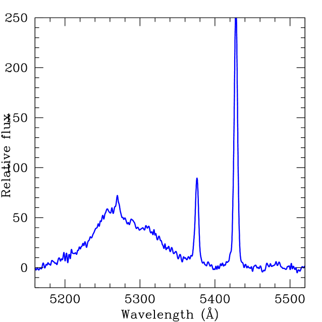
Figure 1: Example of one spectrum that has not been included in the ’clean sample’ on account of its broad $H\beta$ line.

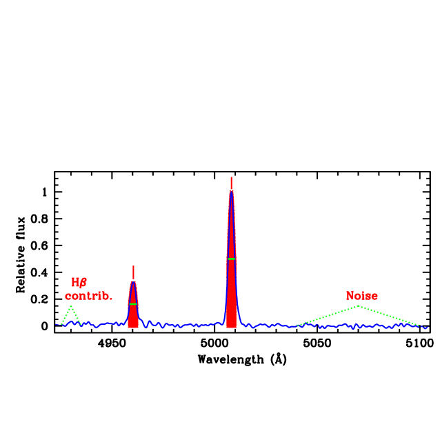
Figure 2: Diagram showing the regions used to compute the centroids and relative fluxes, and the regions used to assess the $H\beta$ residual contamination and the noise in the continuum.

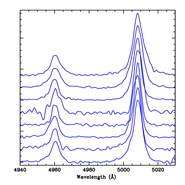
Figure 3: The spectral region around the [OIII] doublet for some of the objects included in the clean sample (see the main text). The spectra have been normalized with respect to the peak of the main [OIII] line.

To estimate the centroids of the lines, we first determined the FWHM of each line and averaged the flux of the pixels within the spectral range covered by that FWHM. We estimate the relative strength of the [OIII] lines with respect to the noise in the adjacent continuum. Such noise was estimated by measuring the continuum rms of each spectrum in the wavelength range 5040–5100 Å (rest frame). We select those objects that have strong ($SNR>20$ in the peak) [OIII] lines. These restrictions provide us with a sub sample (which we refer to hereafter as the “raw sample”) of 3739 objects. The contribution of the H$\beta$ line could in principle produce a blueshift in the estimation of the centroids of the lines, particularly affecting the 4959 Å line. We checked that this contribution could be properly quantified by computing the level of the flux (after subtraction of the continuum) in a spectral region slightly bluer than the position of the [OIII] ($\lambda\lambda$4959) Å line. After many trials we chose the 4925–4935 Å (rest frame) wavelength range to estimate possible residuals of H$\beta$ and remove from the sample those objects with fluxes in that interval above 0.05 the peak value of the [OIII] ($\lambda\lambda$4959) Å line. Fig.1 shows an example of a spectrum that has been rejected on the basis of that criteria. We also eliminated spectra with very wide or double peaked [OIII] lines. Figure 2 shows the different spectral regions used to calculate fluxes and centroids, and to assess potential $H\beta$ residual contamination and the continuum level. We do not impose any further restrictions based on the shape (the presence of asymmetries) of the [OIII] lines. After all these cuts, 1978 spectra remained to constitute our “clean 1” sample. Using this sample we obtain mean $\Delta\alpha/\alpha=(-0.9\pm 2.6)\times 10^{-5}$. The results are very robust against the precise constraints; for instance selecting only those spectra with $SNR>30$ in the peak of the [OIII] lines, we obtain mean $\Delta\alpha/\alpha=(1.9\pm 2.6)\times 10^{-5}$. Figure 3 shows examples of the region centered around the [OIII] doublet of some spectra randomly chosen from this sample. The figure shows that for a given spectrum both lines are well above the noise level, and have similar shapes. A few of them show the presence of asymmetries probably related to the kinematics of the cloud or the presence of multiple clouds. The distributions of centroids of each member of the doublet show similar rms (0.78 Å); this indicates the absence of significant distortions in the estimation of the position of the 4959 Å line due to the relative proximity of the H$\beta$ line. The distribution of the wavelength separation between the centroids of both lines has a rms of 0.11 Å; this indicates that the main factor broadening the distribution of the centroids of the [OIII] lines are absolute spectral shifts which mostly reflect the kinematics ($\leq 150$ km s^-1) of the narrow line clouds where the [OIII] originates.

2.2 Method 2

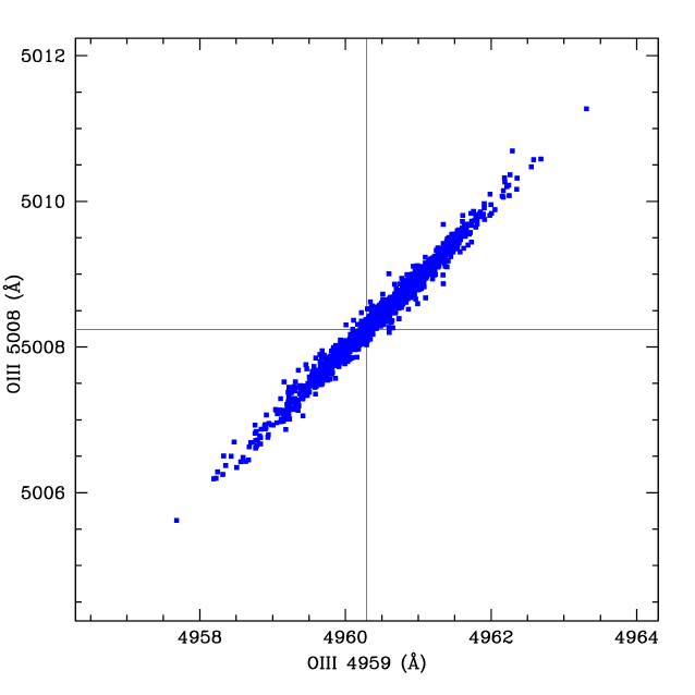
Figure 4: Rest frame position of the two lines of the doublet of [OIII] in the clean sample 2 (see main text). The vertical and horizontal lines indicate the theoretical local values.

The emission lines of OIII (4959 and 5008), and H$\beta$ (narrow and broad components) were simultaneously modeled by single Gaussian each. The wavelength position of each line of the [OIII] doublet was directly estimated as the central position of the corresponding Gaussian. In principle this seems a very simple description of the line profiles, and in many cases produces a poor fit to the data. However, in practice the method takes advantage of the expected similar shape for both lines of the doublet, and removes most of the contribution of H$\beta$ in the spectral region of the [OIII] doublet. After removing the most extreme cases of poor fits, the results are quite consistent and robust. Selecting those spectra in which each of the [OIII] lines are described by Gaussian with peak amplitudes $>20$ the level of the continuum noise, and $\sigma$ within the range 1.4-3.0 Å (rest frame of the [OIII] 5008 line) there were 1568 spectra (’clean sample 2’) from which we obtained $\Delta\alpha/\alpha=(+2.4\pm 2.5)\times 10^{-5}$. Figure 4 shows the wavelengths determined for the spectral position of both lines of [OIII] (to compute the rest frame wavelengths we have used the estimates of redshifts provided by the SDSS database). The wavelengths of both lines lie along a line crossing from the bottom left to the top right and don’t show any systematic effect.

3 Results and discussion

The results obtained by both methods are compatible and quite similar. Both estimations are also compatible with the local value. Most of the spectra included in the clean sample 2 (1223 out of 1568) are also included in the clean sample 1.

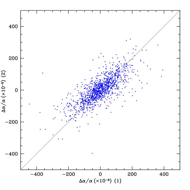
Figure 5: Comparison between the estimations of $\Delta\alpha/\alpha$ by each of the methods used in this paper (see main text for the details).

Fig 5 shows a comparison between the results of both methods. There is a general good agreement between them, although the method of fitting Gaussian tends to be a bit more accurate (the rms of the distributions of $\Delta\alpha/\alpha$ are $9.8\times 10^{-4}$ and $8.0\times 10^{-4}$ for the clean samples 1 and 2 respectively). Then, here after along the paper, we will use the results obtained by the second method.

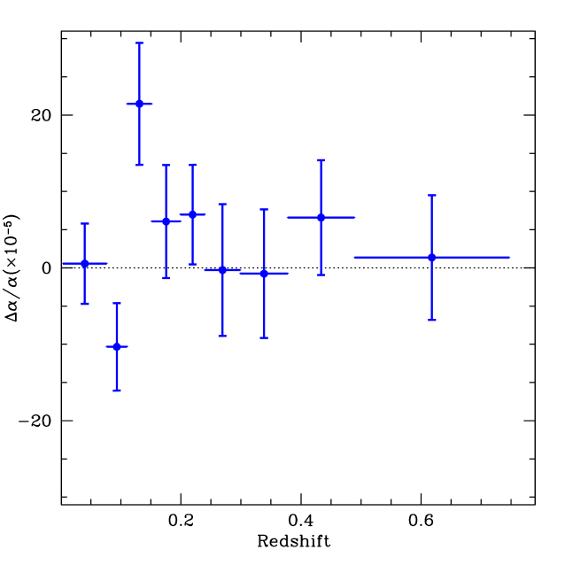
Figure 6: $\Delta\alpha/\alpha$ vs. redshift. Each bin contains the contribution of $\sim 175$ spectra.

To analyze the value of $\Delta\alpha/\alpha$ as a function of redshift (or look-back time) we compute the mean values in redshift interval. This is shown in Fig. 6 and Table 1, which are the main results of this paper. The bins in redshift have been built in order to include approximately the same number (175) of spectra each. Although none of the bins shows a statistical significant departure from zero, the largest deviation is at the 2.7$\sigma$ level in the bin which corresponds to the range in redshift 0.110-0.152. That bin includes those cases in which one of the [OIII] lines lies near the spectral position of the atmospheric OI line. To check for the possible influence of some residual of the OI line in the estimation of the centroids of [OIII] in that range of redshift, we built a new sample excluding those spectra having redshifts in which any of the [OIII] lines is closer than 15 Å to the spectral position of the atmospheric OI line. This new constraint removes 59 spectra. The overall results on $\Delta\alpha/\alpha$ do not change much ($\Delta\alpha/\alpha=(+0.6\pm 2.4)\times 10^{-5}$) using this new clean sample, but the significance of the departure from zero in the corresponding bin in redshift (0.107-0.161) is largely reduced ($\Delta\alpha/\alpha=(+7.0\pm 5.8)\times 10^{-5}$).

The range in redshift spanned by our sample corresponds to a maximum look-back time of 6.6 Gyr, and a mean of 3.0 Gyr. Following Bahcall et al., the mean rate of possible changes is $1/<t>\Delta\alpha/\alpha=(+0.7\pm 0.7)\times 10^{-14}$ yr^-1. A linear fit of $\Delta\alpha/\alpha$ with respect to look-back time gives a slope of $(0.2\pm 1.6)\times 10^{-14}$ yr^-1. All these numbers as a whole do not show any significant evidence of change in $\Delta\alpha/\alpha$ with redshift.

3.1 Line ratios

As a by-product of the analysis we have estimated the value of the line ratio of [OIII]:

$$A\propto\frac{A(5008)\Delta E(5008)}{A(4959)\Delta E(4959)}$$

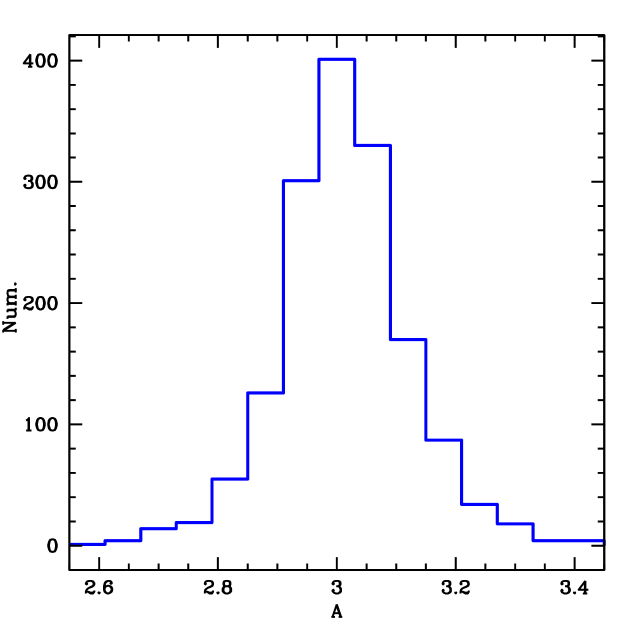
Figure 7: Histogram of the line ratio A of the [OIII] lines.

where $A$ and $\Delta E$ are the transition rates and the energy differences, respectively. The determination of this ratio is interesting as an observational test of calculations from atomic theory where a $\sim 3$ % level of discrepancy exists among the published results (Grupe et al., 2005). We performed numerous tests checking the dependence of $A$ on possible residual contamination from $H\beta$ (see previous section), SNR and [OIII] width. Our best estimation is obtained with the same constraints as those used for the estimation of $\Delta\alpha/\alpha$ using method 2. Fig. 7 shows the histogram of $A$ values for the 1568 spectra included in ’clean sample 2’; the resulting distribution is symmetric, centered at $\sim 3$ and has a standard deviation of 0.10. From that distribution was obtained our best estimation of $A=3.012\pm 0.003\pm 0.010$, where the error bars correspond to the 1$\sigma$ statistical and systematic errors respectively. The systematic errors correspond to uncertainties due to the criteria for selecting the samples. The value obtained agrees with the estimate by Bahcall et al. ($2.99\pm 0.02$), with the measurements $2.993\pm 0.014$ by Dimitrijević et al. (2007) using 62 AGN, and it is compatible with theoretical estimates (2.98) by Storey and Zeippen (2000).

3.2 Other doublets

As pointed out by Bahcall et al. and developed and used by Grupe et al., it is possible to constrain the value of $\alpha$ at cosmological look-back times using doublets of other emission lines that are common in the spectra of QSOs. The most promising are [NeV] ($\lambda\lambda 3346,3426$), [Ne III] ($\lambda\lambda 3869,3968$), [OI] ($\lambda\lambda 6300,6365$), and [SII] ($\lambda\lambda 6717,6731$). The main advantages of the use of these lines is the possibility of extending the study to higher redshifts and of checking the consistency of the results using the [OIII] lines. All of them lie in the optical range and, in the wavelength range of SDSS, can be useful for exploring the ranges in redshifts up to 1.69, 1.31, 0.44 and 0.37 respectively. However, these lines are usually weaker than [OIII] in QSO spectra and some of them also have drawbacks that limit their suitability for these studies. For instance, the lines of the [SII] doublet are relatively close so that further constraints on the width of such lines need to be applied. This pair is also relatively close to the usually very strong and wide H$\alpha$ line in QSOs. On the other hand, the pair of lines for [NeV] and [NeIII] are separated by $\sim$100 Å and then spectral calibration uncertainties might be a more serious concern.

We follow a similar procedure to the one used for [OIII], adapting the constraints on the SNR, possible contributions from neighboring lines, etc., to each specific doublet. As expected, because of the relatively low amplitude of such lines with respect to [OIII], the clean samples of each of these pairs are much smaller, and the sensitivity achieved is poorer than with [OIII]. We decided not to use the [NeV] and [OI] doublets for this analysis because the number of spectra with lines strong enough for a meaningful analysis is very small. In order to have a representative sample of [NeIII] and [SII] we relax our selection criteria to include in the samples all the spectra having SNR$>10$ in the peak of each line of the doublet. Table 2 presents the results for [NeIII] and [SII]. The values found from [SII] are compatible with those from [OIII]. Although the clean sample used in the case of the [SII] contains a relatively high number of spectra (466), the sensitivity achieved is comparatively much lower than the one obtained from [OIII] and [NeIII]. After doing exhaustive tests we found that the relative separation with respect to the width of the lines is the most important factor which limits the use of this pair. Figure 8 $(left)$ shows a comparison between the $\Delta\alpha/\alpha$ values obtained in common spectra between [SII] and [OIII] samples. The figure shows the compatibility of both estimations and the comparatively much large dispersion obtained from the estimations based on [SII].

The values of $\Delta\alpha/\alpha$ obtained from [NeIII] are significantly different from zero. We have checked that this departure from zero keeps along all the range in redshift analyzed using that doublet. The wide range in redshift covered by this sample and the absence of the effect for other lines (for instance, the lines of the [OIII] doublet or the atmospheric OI line) precludes possible systematic errors in wavelength calibration. Figure 8 ($right$) shows a comparison between the estimations of $\Delta\alpha/\alpha$ from the [OIII] and [NeIII] respectively using only common spectra to both samples. Clearly, the results from [NeIII] are not compatible with those from [OIII]. For the distribution of the centroids of each member of the [NeIII] doublet, we have estimated mean values of 3869.61 and 3969.05 Å and rms of 0.51 and 0.58 Å  respectively. The comparison with the theoretical local values (3869.86 and 3968.59 Å respectively) shows discrepancies of 0.25 and 0.46 Å to the blue and to the red respectively. If we restrict the sample according to stronger constraints on the SNR of both lines, these shifts tend to decrease only for the line at 3870 Å. Although this could indicate inaccuracy in the tabulated wavelengths of both transitions, we think the main reason is that the estimated wavelengths for the line [NeIII] (3970 Å) are affected by the proximity of several lines like H$\epsilon$ and the absorption line of CaII-H. Nevertheless, if this is the case it would remain unclear why the rms of the the distributions of both members of the doublet are so similar, and why the shift in the 3970 Å line does not decrease when only spectra with relatively high SNR are considered. Curiously enough, the high value found for $\Delta\alpha/\alpha$ using [NeIII] is similar to the mean value found by Grupe et al. using this pair.

3.3 Comparison with previous studies

In Section 1 we have mentioned the different astronomical methods used to constrain the variation in $\alpha$ with particular emphasis on those based on fine structure splitting. Here, we make comparisons only with previous observations based on the relative splitting of pairs of emission lines in QSOs or AGN in general. The analysis by Bahcall et al. is based on the Early Data Release of SDSS, which comprises a sub sample of the sample analyzed in this paper, so it is worth making a comparison of both studies. There are 38(10) shared objects between the sample of these authors and our raw(clean) sample. Figure 10 shows a comparison between our estimates of $\Delta\alpha/\alpha$ and those by Bahcall et al. The comparison shows a very good agreement between both studies.

The distribution of $\Delta\alpha/\alpha$ obtained from objects in common between our raw sample and the Bahcall et al. sample is similar, while the rms of $\Delta\alpha/\alpha$ from our clean sample is $0.5\times 10^{-3}$, slightly better than the sample of Bahcall et al. ($0.7\times 10^{-3}$). So, although the method and criteria for selecting the samples are quite different from each other, both studies agree quite well. The much higher number of spectra used in this study (1568 in our clean sample) with respect to the 42 objects in the Bahcall et al. sample would allow us in principle to reduce the uncertainty by a factor $\sqrt{1568/42}=6.1$. The result presented by Bahcall et al. is $(0.7\pm 1.4)\times 10^{-4}$ , and therefore our result ($\Delta\alpha/\alpha=(+2.4\pm 2.5)\times 10^{-5}$) improves the sensitivity by a factor $\sim$5, which agrees with statistical expectations.

Grupe et al. (2005) applied the same method to a sample of 14 Sey 1.5 galaxies up to redshift 0.281. These authors include in their analysis the [NeIII], [NeV], [OIII], [OI], and [SII] doublets. They found $\Delta\alpha/\alpha=(1.5\pm 0.7)\times 10^{-3}$, so the result presented in this study improves that sensitivity by a factor $\sim 30$, and the range in redshift covered by a factor $\sim 3$. The method used in this paper to constrain $\alpha$ in the past is about one order of magnitude less sensitive than methods based on the analysis of absorption systems along the line of sight of QSOs. However, as has been discussed above, the method is more transparent, does not require assumptions on the spatial distribution and kinematics of the gas involved, and in general is less subject to systematic errors.

4 Conclusions

The main findings of this work are:

• We have analyzed the sample of 77092 objects classified as QSOs in the SDSS DR6, and from these we have selected a sample of 1568 objects with strong [OIII] emission lines up to redshift 0.80.

• From the relative spectral position in such spectra of the nebular emission of [OIII] $\lambda\lambda 5007$ and 4959 we have estimated a mean value for the fine structure constant of $\Delta\alpha/\alpha=(+2.4\pm 2.5)\times 10^{-5}$ through the last 6.6 Gyr.

• Our analysis improves by a factor $\sim 5-6$ the existing uncertainty in the estimates in the possible change of $\alpha$ using the same method.

• The maximum rate of change in $\Delta\alpha/\alpha$ allowed by our analysis is $(+0.7\pm 0.7)\times 10^{-14}$ yr^-1 in the last 6.6 Gyr.

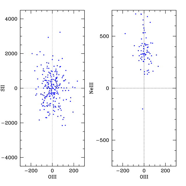
Figure 8: Comparison between the estimations of $\Delta\alpha/\alpha$ obtained from [OIII] and those derived from [SII] ($left$) and [NeIII] ($right$) respectively.

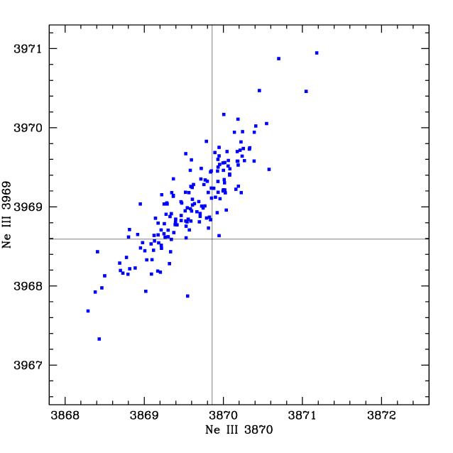
Figure 9: Rest frame position of the two lines of the doublet of [NeIII]. The vertical and horizontal lines indicate the theoretical local values.

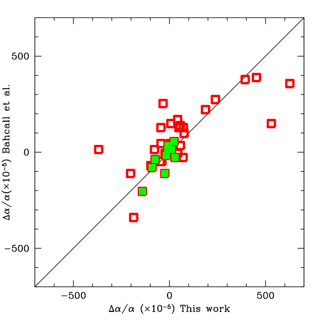
Figure 10: Comparison between the values of $\Delta\alpha/\alpha$ estimated by Bahcall et al. and in this study. Results from spectra included in the raw (clean) sample are plotted as empty (solid) points.

Table 1: $\Delta\alpha/\alpha$ at different redshifts

Redshift	$\Delta\alpha/\alpha$ ($10^{-5})$	1-$\sigma$ errors
0.003 - 0.076	+0.6	5.2
0.076 - 0.110	-10.3	5.7
0.110 - 0.152	+21.5	8.0
0.152 - 0.199	+6.1	7.4
0.199 - 0.240	+7.0	6.5
0.240 - 0.300	-0.3	8.6
0.300 - 0.378	-0.8	8.4
0.378 - 0.490	+6.6	7.5
0.490 - 0.747	+1.4	8.2

Table 2: Results for the different atomic species

Doublet	Spectra	$\Delta\alpha/\alpha$ ($10^{-5})$	1-$\sigma$ errors
OIII	1568	+2.4	2.5
NeIII	168	+358.5	11.2
SII	481	-18.8	41.8

References

- Bahcall and Salpeter (1965) Bahcall, J. N., Salpeter, E. E. 1965, ApJ, 142, 1677
- Bahcall et al. (1967) Bahcall, J. N., Sargent, W. L. W., & Schmidt, M. 1967, ApJ, 149, 211
- Bahcall et al. (2004) Bahcall, J. N., Steinhardt, C. L., & Schlegel, D. 2004, ApJ, 600, 520
- Chand et al. (2004) Chand, H., Srianand, R., Petitjean, P., & Aracil, B. 2004, A&A, 417, 853
- Chand et al. (2005) Chand, H., Petijean, P., Srianand, R., & Aracil, B. 2005, A&A, 430, 47
- Chand et al. (2006) Chand, H., Srianand, R., Petijean, P., Aracil, B., Quast, R., & Reimers, D. 2006, A&A, 451, 45
- Dimitrijević et al. (2007) Dimitrijević, M. S., Popović, L. Č., Kovačević, J., Dačić, M., & Ilić, D. 2007, MNRAS.374.1181
- García-Berro et al. (2007) García-Berro, E., Isern, J., & Kubyshin, Y. A. 2007, A&AR, 14, 113
- Grupe et al. (2005) Grupe, D., Pradhan, A. K., & Frank, S., 2005 AJ, 130, 355
- Ichikawa et al. (2002) Ichikawa, K. & Kawasaki, M. 2002, Phys. Rev., D65, 123511
- Kanekar et al. (2008) Kanekar, N. et al. 2008, Mod. Phys. Lett. A, 23, 2711.
- Landau and Simeone (2008) Landau, S. J., & Simeone, C. 2008, 487, 857
- Levshakov et al. (2005) Levshakov, S. A., Centurion, M., Molaro, P., & D’Odorico, S. 2005, A&A 434, 827
- Levshakov et al. (2007) Levshakov, S. A. et al. 2007, A&A, 466, 1077
- Molaro et al. (2008) Molaro, P., Reimers, D., Agafonova, I. I., & Levshkov, S. A. 2008. Eur. Phys. J. Special Topics, 163, 173
- Murphy et al. (2003) Murphy, M. T., Webb, J. K., & Flambaum, V. V. 2003, MNRAS, 345, 609
- Murphy et al. (2008) Murphy, M. T., Webb, J. K., & Flambaum, V. V. 2008, 384, 1053
- Nakashima et al. (2008) Nakashima, M., Nagata, R., & Yokoyama, J. 2008, PThPh.120.1207
- Srianad et al. (2004) Srianand, R., Chand, H., Petijean, P., & Aracil, B. 2004, Phys. Rev. Lett., 92, 121
- Storey and Zeippen (2000) Storey, P. J.,& Zeippen, C. J. 2000, MNRAS, 312, 813
- Uzan (2003) Uzan, J. P. 2003, Rev. Mod. Phys., 75, 403
- Webb et al. (1999) Webb, J. K., Murphy, M. T., Churchill, C. V., Drinkwater, M. J., & Barrow, J. D. 1999, Phys. Rev. Lett., 82, 884