Modelling cosmological singularity
with compactified Milne space

MODELLING COSMOLOGICAL SINGULARITY
WITH COMPACTIFIED MILNE SPACE

Przemysław Małkiewicz
Institute for Nuclear Studies

Theoretical Physics Department

SUBMITTED IN PARTIAL FULFILLMENT OF THE
REQUIREMENTS FOR THE DEGREE OF
DOCTOR OF PHILOSOPHY IN PHYSICS
SUPERVISED BY DR HAB. WŁODZIMIERZ PIECHOCKI

Abstract

Recent developments in observational cosmology call for understanding the nature of the cosmological singularity (CS). Our work proposes modelling the vicinity of CS by a time dependent orbifold (TDO). Our model makes sense if quantum elementary objects (particle, string, membrane) can go across the singularity of TDO, and our work addresses this issue. We find quantum states of elementary objects, that can propagate in TDO. Our results open door for more detailed examination.

To my parents

Table of Contents

toc

Introduction

Presently available cosmological data suggest that the Universe emerged from a state with extremely high density of physical fields. It is called the cosmological singularity. The data also indicate that known forms of energy and matter comprise only $4\%$ of the makeup of the Universe. The remaining $96\%$ is unknown, called ‘dark’, but its existence is needed to explain the evolution of the Universe [13, 33]. The dark matter, DM, contributes $22\%$ of the mean density. It is introduced to explain the observed dynamics of galaxies and clusters of galaxies. The dark energy, DE, comprises $74\%$ of the density and is responsible for the observed accelerating expansion. These data mean that we know almost nothing about the dominant components of the Universe!

Understanding the nature and the abundance of the DE and DM within the standard model of cosmology, SMC, has difficulties [41, 49]. These difficulties have led many physicists to seek anthropic explanations which, unfortunately, have little predictive power. However, there exist promising models based on the idea of a cyclic evolution of the Universe. There are two main developments based on such an idea: (i) resulting from application of loop quantum gravity [6, 39, 47] to quantization of FRW type Universes, and (ii) inspired by string/M theory [17], the so called cyclic model of the Universe, CMU [42, 43].

The loop quantum cosmology, LQC, shows that the classical cosmological singularity does not occur due to the loop geometry. The Big-Bang of the SMC model is replaced by the Big-Bounce [2, 8, 9, 19]. However, at the present state of development, the LQC is unable to explain the origin of DE and DM.

An alternative model has been proposed by Steinhardt and Turok (ST) [42, 43, 44]. The ST model has been inspired by string/M theories [17]. In its simplest version it assumes that the spacetime can be modelled by the higher dimensional compactified Milne space, $\mathcal{M}_{C}$. The most developed model [43, 42] is one in which spacetime is assumed to be the five dimensional compactified Milne space. In this model the Universe has a form of two 4-dimensional branes separated by a distance which changes periodically its length from zero to some finite value. The Universe changes periodically its dimensionality from five to four, which leads to the evolution of the Universe of the Big-Crunch / Big-Bang type. This model tries to explain the observed properties of the Universe as the result of interaction of ‘our’ brane with the other one. The attractiveness of the ST model is that it potentially provides a complete scenario of the evolution of the universe, one in which the DE and DM play a key role in both the past and the future. The ST model requires DE for its consistency, whereas in the standard model, DE is introduced in a totally ad hoc manner. Demerits of the ST model are extensively discussed in [20]. Response to the criticisms of [20] can be found in [49].

The mathematical structure and self-consistency of the ST model has yet not been fully tested and understood. Such task presents a serious mathematical challenge. It is the subject of the Thesis.

The CMU model has in each of its cycles a quantum phase including the cosmological singularity, CS. The CS plays key role because it joins each two consecutive classical phases. Understanding the nature of the CS has primary importance for the CMU model. Each CS consists of contraction and expansion phases. A physically correct model of the CS, within the framework of string/M theory, should be able to describe propagation of a p-brane, i.e. an elementary object like a particle, string and membrane, from the pre-singularity to post-singularity epoch. This is the most elementary, and fundamental, criterion that should be satisfied. It presents a new criterion for testing the CMU model. Hitherto, most research has focussed on the evolution of scalar perturbations through the CS.

Successful quantization of the dynamics of p-brane will mean that the $\mathcal{M}_{C}$ space is a promising candidate to model the evolution of the Universe at the cosmological singularity. Thus, it could be further used in advanced numerical calculations to explain the data of observational cosmology. Failure in quantization may mean that the CS should be modelled by a spacetime more sophisticated than the $\mathcal{M}_{C}$ space.

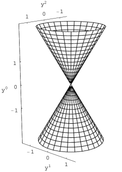
Figure 1: Compactified 2d Milne space embedded in 3d Minkowski space.

The figure $1$ shows the two dimensional $\mathcal{M}_{C}$ space embedded in the three dimensional Minkowski space. It can be specified by the following isometric embedding

$$y^{0}(t,\theta)=t\sqrt{1+r^{2}},~{}~{}~{}~{}y^{1}(t,\theta)=rt\sin(\theta/r),~{}~{}~{}~{}y^{2}(t,\theta)=rt\cos(\theta/r),$$ (0.0.1)

where $(t,\theta)\in\mathbb{R}^{1}\times\mathbb{S}^{1}$ and $0<r\in\mathbb{R}^{1}$ is a constant labelling compactifications . One has

$$\frac{r^{2}}{1+r^{2}}(y^{0})^{2}-(y^{1})^{2}-(y^{2})^{2}=0.$$ (0.0.2)

Eq. (0.0.2) presents two cones with a common vertex at $\>(y^{0},y^{1},y^{2})=(0,0,0)$. The induced metric on (0.0.2) reads

$$ds^{2}=-dt^{2}+t^{2}d\theta^{2}.$$ (0.0.3)

Generalization of the 2-dimensional CM space to the $d+1$ dimensional spacetime has the form

$$ds^{2}=-dt^{2}+t^{2}d\theta^{2}+\delta_{kl}~{}dx^{k}dx^{l},$$ (0.0.4)

where $t,x^{k}\in\mathbb{R}^{1},~{}\theta\in\mathbb{S}^{1}~{}(k=2,\ldots,d)$.

One term in the metric (0.0.4) disappears/appears at $t=0$, thus the $\mathcal{M}_{C}$ space may be used to model the big-crunch/big-bang type singularity. Orbifolding $\mathbb{S}^{1}$ to the segment gives a model of spacetime in the form of two orbifold planes which collide and re-emerge at $t=0$. Such a model of spacetime was used in [17, 42, 43]. Our results apply to both choices of topology of the compact dimension.

The $\mathcal{M}_{C}$ space is an orbifold due to the vertex at $t=0$. The Riemann tensor components equal $0$ for $t\neq 0$. The singularity at $t=0$ is of removable type: any time-like geodesic with $t<0$ can be extended to some time-like geodesic with $t>0$. However, the extension cannot be unique due to the Cauchy problem at $t=0$ for the geodesic equation (the compact dimension shrinks away and reappears at $t=0$).

Chapter 1 Classical dynamics of extended objects

In this chapter we consider classical dynamics of $p$-brane propagating in background spacetime. We formulate it in terms of both Lagrangian and Hamiltonian. The formulations admit gauge symmetry: the action is invariant with respect to diffeomorphisms of $p$-brane’s world-sheet and the Hamiltonian is a sum of first-class constraints. Next we specialize the formalism to the case the embedding spacetime is the compactified Milne space, $\mathcal{M}_{C}$, and analyze classical propagation of extended objects as well as prepare formalism for canonical quantization.

1.1 Lagrangian formalism

A $p$-brane is a $p$-dimensional object, which traces out a $p+1$-dimensional surface, called a $p$-brane’s world-sheet, in the embedding spacetime as it propagates. Both the embedding spacetime and the world-sheet are assumed to be locally Lorentzian.

The Nambu-Goto action is a $p+1$-volume of the p-brane world-sheet and reads:

$$S_{N-G}=-\mu_{p}\int\sqrt{|det(g^{IND}_{ab})|}~{}d^{p+1}\sigma=-\mu_{p}\int\sqrt{-det(\partial_{a}X^{\alpha}\partial_{b}X^{\beta}{g}_{\alpha\beta})}~{}d^{p+1}\sigma,$$ (1.1.1)

where $\mu_{p}$ is a mass per unit $p+1$-volume, $(\sigma^{a})\equiv(\sigma^{0},\sigma^{1},\ldots,\sigma^{p})$ are $p$-brane world-sheet coordinates, $g^{IND}_{ab}$ is an induced metric on the world-sheet, $~{}(X^{\alpha})\equiv(X^{\mu},\Theta)\equiv(T,X^{k},\Theta)\equiv(T,X^{1},\ldots,X^{d-1},\Theta)$ are the embedding functions of a $p$-brane, i.e. $X^{\alpha}=X^{\alpha}(\sigma^{0},\ldots,\sigma^{p}$), in $d+1$ dimensional background spacetime with metric ${g}_{\alpha\beta}$. As a subcase for $p=0$ the formula (1.1.1) includes the action of a particle moving in a background spacetime. The least action principle, i.e. $\delta S_{N-G}=0$, applied to (1.1.1) leads to the following equations of motion:

$$\partial_{a}(\frac{\partial_{b}X^{\alpha}\partial_{b}X^{\beta}g_{\alpha\beta}}{\sqrt{-det(\partial_{a}X^{\alpha}\partial_{b}X^{\beta}{g}_{\alpha\beta})}}\partial_{a}X_{\mu}-\frac{\partial_{a}X^{\alpha}\partial_{b}X^{\beta}g_{\alpha\beta}}{\sqrt{-det(\partial_{a}X^{\alpha}\partial_{b}X^{\beta}{g}_{\alpha\beta})}}\partial_{b}X_{\mu})$$

$$-\frac{(\partial_{a}X^{\alpha}\partial_{a}X^{\beta}g_{\alpha\beta})\partial_{b}X^{\alpha}\partial_{b}X^{\beta}-(\partial_{a}X^{\alpha}\partial_{b}X^{\beta}g_{\alpha\beta})\partial_{a}X^{\alpha}\partial_{b}X^{\beta}}{2\sqrt{-det(\partial_{a}X^{\alpha}\partial_{b}X^{\beta}{g}_{\alpha\beta})}}g_{\alpha\beta,\mu}=0.$$ (1.1.2)

The above equations (1.1.2) are undetermined (not only because of unspecified initial/boundary conditions but) due to freedom in the choice of parameters $(\sigma^{a})$ (for $a=0,\dots,p$) as consequence of re-parametrization invariance of the action (1.1.1). A convenient setting for gauge fixing is the Polyakov action.

The Polyakov action for a test $p$-brane embedded in a background spacetime with metric $g_{\alpha\beta}$ has the form

$$S_{P}=-\frac{1}{2}\mu_{p}\int d^{p+1}\sigma\sqrt{-\gamma}\;\big{(}\gamma^{ab}\partial_{a}X^{\alpha}\partial_{b}X^{\beta}g_{\alpha\beta}-(p-1)\big{)},$$ (1.1.3)

where $\gamma_{ab}$ is the $p$-brane world-sheet metric, $\gamma:=det[\gamma_{ab}]$. The least action principle applied to (1.1.3) produces the following equations of motion:

$$\partial_{a}(\sqrt{-\gamma}\gamma^{ab}\partial_{b}X_{\mu})=\frac{1}{2}\sqrt{-\gamma}\gamma^{ab}\partial_{a}X^{\alpha}\partial_{b}X^{\beta}g_{\alpha\beta,\mu},$$ (1.1.4)

$$\partial_{a}X^{\alpha}\partial_{b}X^{\beta}~{}g_{\alpha\beta}-\frac{1}{2}\gamma_{ab}\gamma^{cd}\partial_{c}X^{\alpha}\partial_{d}X^{\beta}~{}g_{\alpha\beta}=0.$$ (1.1.5)

The above equations are in full equivalence with the equations (1.1.2). But in this case it is convenient to fix a gauge by specifying the fields $\gamma_{ab}$ to some extent. For example, in case of a string there are two ways of doing it:

1. Partially fixed gauge: one sets the matrix $\sqrt{\gamma}\gamma^{ab}$ as functions of $(\sigma^{a})$; afterwards there are still conformal isometries of the world-sheet allowed in this setting and the least action principle wrt fields $X^{\alpha}$ is still applicable.

2. Fully fixed gauge: one sets lapse and shift function like in General Relativity; one fixes this gauge at the level of equations of motion.

In the next section we will move to the Hamiltonian formalism, which comes from applying a Legandre transormation to the Nambu-Goto or Polyakov action.

1.2 Hamiltonian formalism

This section introduces Hamiltonian formalism with a brief review of Dirac’s procedure for constrained systems. The constraints are phase space functions that are gauge generators, i.e. they are manifestation of re-parametrization invariance of the corresponding action.

Let us denote a position-velocity space of a system by $(q,\dot{q})$. Let us also assume that the Legendre transformation $(q,\dot{q})\mapsto(q,p=\frac{\partial L}{\partial\dot{q}})$ is singular, i.e. there exist relations of the form $\Phi_{a}(q,p)=0$. The consistency condition requires:

$$\{\Phi_{a},H\}\approx 0,~{}~{}\{\Phi_{a},\Phi_{b}\}\approx 0,$$

where $H=p\dot{q}-L$, ’$\approx$’ denotes equality holding on the surface $\Phi(q,p)=0$ and $a,b=1,2,\dots$ The satisfaction of the above equation may require introduction of new relations $\Upsilon_{a}(q,p)=0$, called secondary constraints. One applies the consistency condition until it produces no more new constraints. Now the constraints are first-class, which means they close to a Poisson algebra (for more details see [12, 15]).

Sometimes it is possible to reduce the number of conjugate pairs by solving some of the constraints. This is called reduced phase space formalism and it is used here.

It has been found [34] that the total Hamiltonian, $H_{T}$, corresponding to the action (1.1.1) is the following

$$H_{T}=\int d^{p}\sigma\mathcal{H}_{T},~{}~{}~{}~{}\mathcal{H}_{T}:=AC+A^{i}C_{i},~{}~{}~{}~{}~{}i=1,\ldots,p$$ (1.2.1)

where $A=A(\sigma^{a})$ and $A^{i}=A^{i}(\sigma^{a})$ are any functions of $p$-volume coordinates,

$$C:=\Pi_{\alpha}\Pi_{\beta}g^{\alpha\beta}+\mu_{p}^{2}\;det[\partial_{a}X^{\alpha}\partial_{b}X^{\beta}g_{\alpha\beta}]\approx 0,$$ (1.2.2)

$$C_{i}:=\partial_{i}X^{\alpha}\Pi_{\alpha}\approx 0,$$ (1.2.3)

and where $\Pi_{\alpha}$ are the canonical momenta corresponding to $X^{\alpha}$. Equations (1.2.2) and (1.2.3) define the first-class constraints of the system.

The Hamilton equations are

$$\dot{X}^{\alpha}\equiv\frac{\partial{X}^{\alpha}}{\partial\tau}=\{X^{\alpha},H_{T}\},~{}~{}~{}~{}~{}~{}\dot{\Pi}_{\alpha}\equiv\frac{\partial{\Pi}_{\alpha}}{\partial\tau}=\{\Pi_{\alpha},H_{T}\},~{}~{}~{}~{}~{}~{}\tau\equiv\sigma^{0},$$ (1.2.4)

where the Poisson bracket is defined by

$$\{\cdot,\cdot\}:=\int d^{p}\sigma\Big{(}\frac{\partial\cdot}{\partial X^{\alpha}}\frac{\partial\cdot}{\partial\Pi_{\alpha}}-\frac{\partial\cdot}{\partial\Pi_{\alpha}}\frac{\partial\cdot}{\partial X^{\alpha}}\Big{)}.$$ (1.2.5)

One finds that the constraints satisfy the following algebra:

$$\{C(f),C(g)\}=4\mu_{p}^{2}C_{i}(hh^{ij}(fg_{,j}-gf_{{}^{\prime}j}))$$

$$\{C_{i}(f^{i}),C(g)\}=C(f^{i}g_{,i}-gf^{i}_{,i})$$ (1.2.6)

$$\{C_{i}(f^{i}),C_{i}(g^{i})\}=C_{i}(f^{j}g^{i}_{,j}-g^{j}f^{i}_{,j})$$

where $h_{ab}:=det[\partial_{a}X^{\alpha}\partial_{b}X^{\beta}g_{\alpha\beta}]$, $h:=det[h_{ab}]$ and the smeared phase space function $A(f)$ is defined as:

$${A}(f):=\int_{\Sigma}d^{p}\sigma\;f(\sigma^{a})A(X^{\mu},\Pi_{\mu}).$$ (1.2.7)

1.3 A $p$-brane in compactified Milne Universe

In this section we will specialize the general formulas gathered in previous sections to the cases of the lowest dimensional objects, i.e. particle, string and membrane, propagating in the compactified Milne space, $\mathcal{M}_{C}$. We will solve the equations of motion in case of particle and string. We will also introduce dimensionally reduced states that are possible for string and membrane. These reductions will play a role in canonical formulation, prior to quantization performed in the next chapter.

1.3.1 Particle

For the sake of clarity we restrict the following analysis to the significant dimensions of the $\mathcal{M}_{C}$ space, i.e. the time and the disappearing/appearing dimensions. In other words, we use the metric

$$ds^{2}=-dt^{2}+t^{2}d\theta^{2}.$$ (1.3.1)

The Lagrangian formalism

The Polyakov action, $S_{P}$, describing a relativistic test particle of mass $m$ in a gravitational field $g_{\alpha\beta}~{}~{}(\alpha,\beta=0,1)$ is defined by (see (1.1.3) and [24, 25]):

$$S_{P}=\int d\tau\>L(\tau),~{}~{}~{}~{}~{}~{}~{}L(\tau):=\frac{m}{2}\>(\frac{\dot{X}^{\alpha}\dot{X}^{\beta}}{e}g_{\alpha\beta}-e),~{}~{}~{}~{}\dot{X}^{\alpha}:=dX^{\alpha}/d\tau,$$ (1.3.2)

where $\tau$ is an evolution parameter, $e(\tau)$ denotes the ‘einbein’ on the world-line ($e(\tau)\equiv\sqrt{\gamma}$ in (1.1.3)), $X^{0}$ and $X^{1}$ are time and space coordinates, respectively.

In the specified metric (1.3.1) the Lagrangian in (1.3.2) reads

$$L(\tau)=\frac{m}{2e}\>(T^{2}\dot{\Theta}^{2}-\dot{T}^{2}-e^{2}).$$ (1.3.3)

For the Lagrangian (1.3.3) the equations of motion read

$$\frac{d}{d\tau}\bigg{(}\frac{mT^{2}\dot{\Theta}}{e}\bigg{)}=0,~{}~{}~{}~{}~{}~{}\ddot{T}-\bigg{(}\frac{\dot{e}}{e}\bigg{)}\dot{T}+\dot{\Theta}^{2}T=0,~{}~{}~{}~{}~{}~{}e^{2}=\dot{T}^{2}-T^{2}\dot{\Theta}^{2}.$$ (1.3.4)

The solution to (1.3.4) may be expressed in a gauge-invariant manner:

$$\Theta(T)=-\int\frac{d(\frac{c_{1}}{mT})}{\sqrt{1+(\frac{c_{1}}{mT})^{2}}}=-\textrm{arsinh}\bigg{(}\frac{c_{1}}{mT}\bigg{)}+c_{2},~{}~{}~{}~{}c_{1}\in\mathbb{R},~{}~{}0\leq c_{2}<2\pi.$$ (1.3.5)

Now one observes that for $c_{1}\neq 0$ particle winds infinitely many times around $\theta$-dimension as $t\rightarrow 0~{}$ and the value of $\frac{d\Theta}{dT}$ is not well-defined for $t=0$. If we distinguish between points of different value of $\theta$ for $t=0$, then the particle becomes topologically (of length equal to zero) a string at the singularity, since every point in the line $(t,\theta)=(0,\mathbb{S}^{1})$ is the $t\rightarrow 0~{}$ limit of the formula (2.4.25). Therefore, the dynamics has no unique extension beyond the singularity no matter which topology one ascribes to the point(s) $t=0$.

We now see that there are two different aspects of non-uniqueness of the particle’s classical propagation across the singularity:

1. There is no coordinate system covering a neighborhood of the singularity unless we assign the topology of circle to it.

2. Even if we do this the particle cannot be traced down to the very singularity since it winds infinitely many times around the compact dimension.

Taking into account the above one may say that only the $c_{1}=0$ states can be uniquely extended beyond the singularity.

The Hamiltonian formalism

In the Hamiltonian formalism we obtain the constraint (see (1.2.2) and [22]):

$$C:=\Pi_{a}\Pi_{b}g^{ab}+m^{2}=(\Pi_{\theta}/T)^{2}-(\Pi_{t})^{2}+m^{2},$$ (1.3.6)

where $\Pi_{t}:=\partial L/\partial\dot{T}\>$ and $\Pi_{\theta}:=\partial L/\partial\dot{\Theta}\>$ are canonical momenta. The Hamiltonian $H_{T}=A~{}C$ (where $A$ is an arbitrary function of $\tau$) gives the equations of motion:

$$\dot{\Theta}=\frac{2A(\tau)}{T^{2}}\Pi_{\theta}, ~{}~{}~{}~{}\dot{T}=2A(\tau)\Pi_{t},$$ (1.3.7)

$$\dot{\Pi}_{\theta}=0, ~{}~{}~{}~{}\dot{\Pi}_{t}=\frac{2A(\tau)}{T^{3}}\Pi_{\theta}^{2}.$$ (1.3.8)

Thus, during evolution of the system $\Pi_{\theta}$ is conserved. Owing to the constraint (1.3.6), $\Pi_{t}$ blows up as $T\rightarrow 0~{}$ for $\Pi_{\theta}\neq 0$. This is a real problem, i.e. it cannot be avoided by a suitable choice of coordinates. It is called the ’blue-shift’ effect.

However, trajectories of a test particle, i.e. nonphysical particle, coincide (by definition) with time-like geodesics of an empty spacetime, and there is no obstacle for such geodesics to reach/leave the singularity. It is clear that such an extension cannot be unique because at $t=0$ the Cauchy problem for the geodesic equation is not well defined. Therefore the $\Pi_{\theta}=0$ states are distinguished as the only deterministically extendable ones.

We postpone further discussion to the next chapter, where we will deal with quantum theory.

1.3.2 String

The Lagrangian formalism

One can check that using the embedding functions $T$ and $\Theta$ for expressing dynamics of a string even in the most convenient gauges produces a difficult system of coupled non-linear equations. Therefore we will proceed in a different way [28] and use the local flatness of the $\mathcal{M}_{C}$ space, a fact, that is transparent in the coordinates:

$$x^{0}=t\cosh{\theta},~{}~{}~{}~{}~{}~{}x^{1}=t\sinh{\theta}.$$ (1.3.9)

This strategy is to be effective because the solutions to the dynamics of string in Minkowski spacetime are already known.

An action describing a test string in a fixed background spacetime with metric $g_{\mu\nu}$ may be given by the Polyakov action (see (1.1.3)):

$$S_{P}=-\frac{1}{2}\mu_{1}\int d\tau d\sigma~{}\sqrt{-\gamma}~{}\gamma^{ab}~{}X_{,a}^{\mu}X^{\nu}_{,b}~{}g_{\mu\nu},$$ (1.3.10)

where $\mu_{1}$ is a mass per unit length, $\gamma_{ab}$ is the string world-sheet metric, $\gamma:=det[\gamma_{ab}]$ and where $X^{\mu}=(T,X^{1},\dots,X^{d})$.

Inserting $\sqrt{-\gamma}~{}\gamma^{ab}:=\eta^{ab}$ (which is a special choice of gauge on the string’s world-sheet) and $g_{\mu\nu}:=\eta_{\mu\nu}$ into (1.3.10) leads to, after applying variational principle, the following equations of motion

$$\partial_{\tau}^{2}X^{\mu}-\partial_{\sigma}^{2}X^{\mu}=0,$$ (1.3.11)

plus a boundary condition. Hence, the string’s propagation in Minkowski space is described by

$$X^{\mu}(\tau,\sigma)=X^{\mu}_{+}(\tau+\sigma)+X^{\mu}_{-}(\tau-\sigma),$$ (1.3.12)

$$\partial_{\tau}X^{\mu}\partial_{\tau}X_{\mu}+\partial_{\sigma}X^{\mu}\partial_{\sigma}X_{\mu}=0,~{}~{}~{}~{}~{}~{}\partial_{\tau}X^{\mu}\partial_{\sigma}X_{\mu}=0,$$ (1.3.13)

where $X_{\pm}^{\mu}$ are any functions. The equations (1.3.13) are gauge constraints. We can make use of these solutions to construct string solutions in the $\mathcal{M}_{C}$ space which wind round the compact dimension, and therefore can be expressed in terms of a function $\overline{X}(t,\theta)$, where $\overline{X}:=(X^{2},X^{3},\texttt{\ldots},X^{d})$.

It follows from (1.3.9) that the range of this mapping has a nontrivial topology due to the existence of the singular point $(x^{0},x^{1})=(0,0)$ (see figure 1.1). Combining this property with the general solution (1.3.12), we inevitably arrive to the following topology condition

$$x^{0}=f(\tau+\sigma)-f(-\tau+\sigma),~{}~{}~{}~{}~{}x^{1}=g(\tau+\sigma)-g(-\tau+\sigma),$$ (1.3.14)

where $f$ and $g$ are any functions. One can always arrive to the above form by performing an appropriate conformal transformation $\sigma_{\pm}\rightarrow\widetilde{\sigma_{\pm}}(\sigma_{\pm})$, where $\sigma_{\pm}=\sigma\pm\tau$. More precisely, let us make the conformal transformation on the solution (1.3.12) to get $X^{0}=f(\tau+\sigma)-f(-\tau+\sigma)$. One can verify that other forms of $X^{0}$ are excluded. It follows from (1.3.9) that we have the implication: $(X^{0}=0)\Rightarrow(X^{1}=0)$. This means that for $\tau=0$ we have $X^{1}=0$, which leads to $X^{1}=g(\tau+\sigma)-g(-\tau+\sigma)$.

Figure 1.1: Singular property of the map $(\tau,\sigma)\longrightarrow(x^{0},x^{1})$. The map is invertible for $\tau\neq 0$, and non-invertible for $\tau=0$.

Now, let us impose the symmetry condition on the remaining $X^{k},(k>1)$ embedding functions. Due to the assumption made earlier, $X^{k}$ are functions of $t$ and $\theta$, i.e. $X^{k}(\tau,\sigma)=\widetilde{X}^{k}(t(\tau,\sigma),\theta(\tau,\sigma))$ and are to be periodic in $\theta$. It follows from (1.3.14) that

$$\theta=\textrm{arctanh}\Big{(}\frac{g(\sigma_{+})-g(-\sigma_{-})}{f(\sigma_{+})-f(-\sigma_{-})}\Big{)}$$ (1.3.15)

$$t=\textrm{sgn}(\tau)~{}\sqrt{(f(\sigma_{+})-f(-\sigma_{-}))^{2}-(g(\sigma_{+})-g(-\sigma_{-}))^{2}}$$ (1.3.16)

So the symmetry condition states that $X^{k}=X^{k}_{+}(\sigma_{+})+X^{k}_{-}(\sigma_{-})$ is periodic in $\theta=\textrm{arctanh}(\frac{g(\sigma_{+})-g(-\sigma_{-})}{f(\sigma_{+})-f(-\sigma_{-})})$. In other words, we should determine $X^{k}_{+}$ and $X^{k}_{-}$ from

$$X^{k}_{+}(\sigma_{+})+X^{k}_{-}(\sigma_{-})=\sum_{n}a_{n}^{k}(t)\exp\big{(}\imath\frac{2\pi n}{\beta}\theta\big{)},$$ (1.3.17)

where $a_{n}^{k}$ are functions of $t$ whose exact form we will discover below. It may seem to be impossible to satisfy these conditions. One obstacle is due to the fact that on the left-hand side we have a sum of functions of a single variable, while on the right-hand side there is a sum of functions which depend in a rather complicated way on both variables. However, we can compare both sides of (1.3.17) at a line. In this way one can rule out one of the variables and compare functions dependent on just a single variable. The procedure rests upon the fact that the dynamics is governed by a second order differential equation (1.3.11), and thus it is sufficient to satisfy the symmetry condition by specifying $X^{k}$, $\partial_{t}X^{k}$ on a single Cauchy’s line. We choose it to be the singularity, i.e. the line $\sigma_{+}=-\sigma_{-}$, or equivalently $t=0$. One can check that as $\sigma_{+}+\sigma_{-}\rightarrow 0$, one gets $\theta\rightarrow\textrm{arctanh}(g^{\prime}/f^{\prime})$, where the prime indicates differentiation with respect to an arbitrary parameter.

Our strategy consists in the imposition of the two conditions:

$$\lim_{\sigma_{+}+\sigma_{-}\rightarrow 0}X^{k}=X^{k}_{+}(\sigma)+X^{k}_{-}(\sigma)=\sum_{n}a_{n}^{k}(0)\exp\big{(}\imath\frac{2\pi n}{\beta}\textrm{arctanh}\big{(}\frac{g^{\prime}}{f^{\prime}}\big{)}(\sigma)\big{)},$$ (1.3.18)

$$\lim_{\sigma_{+}+\sigma_{-}\rightarrow 0}\partial_{t}X^{k}=\partial_{t}X^{k}_{+}(\sigma)+\partial_{t}X^{k}_{-}(\sigma)=\sum_{n}\dot{a}_{n}^{k}(0)\exp\big{(}\imath\frac{2\pi n}{\beta}\textrm{arctanh}\big{(}\frac{g^{\prime}}{f^{\prime}}\big{)}(\sigma)\big{)}.~{}~{}~{}~{}$$ (1.3.19)

In this way we get the following simplifications: (i) as we compare functions on a line we in fact compare functions of a single variable, (ii) since we choose the line $t=0$, we obtain a rather simple form on the right-hand side in the form of a periodic function of $\theta=\arctan(g^{\prime}/f^{\prime})$. The only remaining work to be done is to find the operator $\partial_{t}$ in the limit $~{}\sigma_{+}+\sigma_{-}\rightarrow 0$.

One can check (see the paper [28]) that

$$\partial_{t} = \frac{\partial_{-}\theta}{\partial_{+}t\partial_{-}\theta-\partial_{-}t\partial_{+}\theta}~{}\partial_{+}-\frac{\partial_{+}\theta}{\partial_{+}t\partial_{-}\theta-\partial_{-}t\partial_{+}\theta}~{}\partial_{-}$$

in the limit $~{}\sigma_{+}+\sigma_{-}\rightarrow 0$ turns to be

$$\partial_{t} \longrightarrow \frac{1}{2\sqrt{(f^{\prime})^{2}-(g^{\prime})^{2}}}(\partial_{+}+\partial_{-})~{}~{}\Big{|}_{\sigma_{+}=-\sigma_{-}}.$$ (1.3.20)

Now it is straightforward to check that application the conditions (1.3.18) and (1.3.19) render

$$X^{0} = q\sinh(\sigma_{+})+q\sinh(\sigma_{-}),$$ (1.3.21)

$$X^{1} = q\cosh(\sigma_{+})-q\cosh(\sigma_{-}),$$ (1.3.22)

$$X^{k} = \sum_{n}a_{n+}^{k}\exp\big{(}\imath\frac{2\pi n}{\beta}\sigma_{+}\big{)}$$ (1.3.23)

$$+ \sum_{n}a_{n-}^{k}\exp\big{(}\imath\frac{2\pi n}{\beta}\sigma_{-}\big{)}+{c_{0}^{k}}(\sigma_{+}+\sigma_{-}),$$

where $k>1$. These solutions should satisfy the gauge conditions (1.3.13), which now takes the form

$$\partial_{+}X_{k}\partial_{+}X^{k}=q^{2}=\partial_{-}X_{k}\partial_{-}X^{k}.$$ (1.3.24)

Now one can find that the solutions as functions of $t$ and $\theta$ have the form

$$X^{k}(t,\theta) = \sum_{n}\Big{(}a_{n+}^{k}e^{\imath\frac{2\pi n}{\beta}\textrm{arcsinh}\big{(}\frac{t}{2q}\big{)}}+a_{n-}^{k}e^{-\imath\frac{2\pi n}{\beta}\textrm{arcsinh}\big{(}\frac{t}{2q}\big{)}}\Big{)}\exp\big{(}\imath\frac{2\pi n}{\beta}\theta\big{)}$$ (1.3.25)

$$+ 2c_{0}^{k}\textrm{arcsinh}\Big{(}\frac{t}{2q}\Big{)},$$

where $n$ denotes $n$-th excitation. The number of arbitrary constants in (1.3.25) can be reduced by the imposition of the gauge condition (1.3.24).

Equation (1.3.25) defines the solution corresponding to the compactification of one space dimension to $S^{1}$. The solution corresponding to the compactification to a segment, can be obtained from (1.3.25) by the imposition of the condition $X^{k}(t,\theta)=X^{k}(t,-\theta)$, which leads to $a^{k}_{n}=-b^{k}_{n}$ and $\varphi_{n}^{k}=-\phi_{n}^{k}$, where $\theta\in[0,\beta/2]$.

The general solution (1.3.25) shows that the propagation of a string through the cosmological singularity is not only continuous and unique, but also analytic. Solution in the $\mathcal{M}_{C}$ space is as regular as in the case of the Minkowski space.

The imposition of the gauge constraint (1.3.24) on the infinite set of functions given by (1.3.25) produces an infinite variety of physical states. This procedure goes exactly in the same way as for a closed string in Minkowski spacetime, but with a smaller number of degrees of freedom due to the condition that the string is winding around the compact dimension.

The Hamiltonian formalism

There is no need to repeat all the results from the Lagrangian formalism in the Hamiltonian formalism. Our need for the Hamiltonian formalism comes from our intention to quantize the system canonically. Although we have found all the solutions for a string winding round the compact dimension, we are going to quantize only special states, i.e. strings which are winding uniformly. In this way we reduce a field theory (with infinitely many degrees of freedom) to a mechanical system and thus multiply our chances for success.

We analyze the dynamics of a string in the zero-mode (the lowest energy state) which is winding around the $\theta$-dimension [21, 26]. The string in such a state is defined by the condition

$$\sigma^{1}:=\theta~{}~{}~{}~{}~{}~{}\mbox{and}~{}~{}~{}~{}~{}\partial_{\theta}X^{\mu}=0=\partial_{\theta}\Pi_{\mu},$$ (1.3.26)

One can show that the condition (1.3.26) eliminates the canonical pair $(\Theta,\Pi_{\theta})$ and thus reduces the constraints (see (1.2.2), (1.2.3) and [21, 26]):

$$C=\Pi_{\mu}(\tau)\;\Pi_{\nu}(\tau)\;\eta^{\mu\nu}+\check{\mu}_{1}^{2}\;T^{2}(\tau)\approx 0,~{}~{}~{}~{}~{}~{}C_{1}\equiv 0,$$ (1.3.27)

where $\check{\mu}_{1}\equiv\theta_{0}\mu_{1}$ and $X^{\mu}$ no longer includes the embedding functions corresponding to the compact dimension $\theta$.

Let us solve the dynamics. The equations of motion (1.2.4) read

$$\dot{\Pi}_{t}(\tau)=-2A(\tau)\;\check{\mu}_{1}^{2}\;T(\tau),~{}~{}~{}~{}~{}~{}\dot{\Pi}_{k}(\tau)=0,$$ (1.3.28)

and

$$\dot{T}(\tau)=-2A(\tau)\;\Pi_{t}(\tau),~{}~{}~{}~{}~{}~{}\dot{X}^{k}(\tau)=2A(\tau)\;\Pi_{k}(\tau),$$ (1.3.29)

where $A=A(\tau)$ is any regular function.

It can be verified that in the gauge $A(\tau)=1$, the solutions are

$$\Pi_{t}(\tau)=b_{1}\exp(2\check{\mu}_{1}\tau)+b_{2}\exp(-2\check{\mu}_{1}\tau),~{}~{}~{}~{}~{}~{}\Pi_{k}(\tau)=\Pi_{0k},$$ (1.3.30)

where $~{}\;b_{1},b_{2},\Pi_{0k}\in\mathbb{R}$, and

$$T(\tau)=a_{1}\exp(2\check{\mu}_{1}\tau)+a_{2}\exp(-2\check{\mu}_{1}\tau),~{}~{}~{}~{}~{}X^{k}(\tau)=X^{k}_{0}+2\Pi_{0k}\;\tau,$$ (1.3.31)

where $\;a_{1},a_{2},X^{k}_{0}\in\mathbb{R}$.

To analyze the propagation of a string across the singularity $t=0$, we eliminate $\tau$ from (1.3.30) and (1.3.31). Making the choice of $a_{1}$ and $a_{2}$ in such a way that $a_{1}a_{2}<0$ leads to one-to-one relation between $T$ and $\tau$. For instance, one may put

$$a_{1}=-a_{2}=\sqrt{\Pi_{0}^{k}\Pi_{0k}}/2\check{\mu}_{1},$$ (1.3.32)

that gives

$$T(\tau)=\sqrt{\Pi_{0}^{k}\Pi_{0k}}\;\sinh(2\check{\mu}_{1}\;\tau)/\check{\mu}_{1},$$ (1.3.33)

which can be rewritten as

$$\tau=\frac{1}{2\check{\mu}_{1}}\sinh^{-1}\Big{(}\frac{\check{\mu}_{1}}{\sqrt{\Pi_{0}^{k}\Pi_{0k}}}\;t\Big{)},$$ (1.3.34)

due to $T=t$. The insertion of (1.3.34) into (1.3.31) gives

$$X^{k}(t)=X^{k}_{0}+\frac{\Pi_{0}^{k}}{\check{\mu}_{1}}\sinh^{-1}\Big{(}\frac{\check{\mu}_{1}}{\sqrt{\Pi_{0}^{k}\Pi_{0k}}}\;t\Big{)}.$$ (1.3.35)

The solution (1.3.35) is bounded and continuous at the singularity. Thus, the classical dynamics of the zero-mode winding string is well defined in the $\mathcal{M}_{C}$ space. In fact, it corresponds to the solution (1.3.25) for

$$q=\frac{\sqrt{\Pi_{0}^{k}\Pi_{0k}}}{2\check{\mu}_{1}},~{}~{}c^{k}_{0}=\frac{\Pi^{k}_{0}}{2\check{\mu}_{1}},~{}~{}a^{k}_{0+}+a^{k}_{0-}=X^{k}_{0}.$$ (1.3.36)

One may note that in case the string is winded uniformly around the compact dimension the propagation is unique and smooth through the singularity no matter whether it has circle or point topology.

Let us once more distinguish between two different topologies one may assign to compactified Milne space, for which the line element reads (we omit higher dimensions):

$$ds^{2}=-dt^{2}+t^{2}d\theta^{2}.$$ (1.3.37)

As it is clear from the above formula, for $t=0$ the metric is degenerate and there is a singularity. We say the singularity has point topology if there is a single point with $t=0$. On the contrary, we say the singularity has circle topology if there is a continuum of points with $t=0$, each enumerated with different value of $\theta$. Clearly, the distance between these points is equal to zero.

1.3.3 Membrane

The case of a membrane constitutes the most difficult part of our classical analysis. We restrict ourselves to considering the states that are winding uniformly round the compact dimension both in the Lagrangian and Hamiltonian formulation. In the Lagrangian formalism we will limit our discussion to stating the equations of motion and laws of conservation in the gauge, which as we believe, is the most promising for finding the solutions. In the Hamiltonian formalism the mentioned reduction leads to an algebra of two constraints, which we will rephrase in a form convenient for Dirac’s quantization.

The Lagrangian formalism

The Nambu-Goto action for a membrane in the $\mathcal{M}_{C}$ space reads

$$S_{NG} = -\mu_{2}\int d^{3}\sigma\sqrt{-det(\partial_{a}X^{\mu}\partial_{b}X^{\nu}g_{\mu\nu})}$$ (1.3.38)

$$= -\mu_{2}\int d^{3}\sigma\sqrt{-det(-\partial_{a}T\partial_{b}T+T^{2}\partial_{a}\Theta\partial_{b}\Theta+\partial_{a}X^{k}\partial_{b}X_{k})}$$

where $(T,\Theta,X^{k})$ are embedding functions of the membrane corresponding to the spacetime coordinates $(t,\theta,x^{k})$ respectively.

An action $S_{NG}$ in the lowest energy winding mode, defined by (1.3.26), has the form [29]

$$S_{NG} = -\mu_{2}\theta_{0}\int d^{2}\sigma\sqrt{-T^{2}det(-\partial_{a}T\partial_{b}T+\partial_{a}X^{k}\partial_{b}X_{k})}$$ (1.3.39)

$$= -\mu_{2}\theta_{0}\int d^{2}\sigma\sqrt{-det(\partial_{a}X^{\alpha}\partial_{b}X^{\beta}\widetilde{g}_{\alpha\beta})}.$$

where $a,b\in\{0,1\}$,  $\widetilde{g}_{\alpha\beta}=T\eta_{\alpha\beta}$ and $\theta_{0}=\int d\theta$. Now it is clear that the dynamics of a membrane in the state (1.3.26) is equivalent to the dynamics of a string with tension $\mu_{2}\theta_{0}$ in the spacetime with the metric $\widetilde{g}_{\alpha\beta}$.

The Nambu-Goto action (1.3.39) is equivalent to the Polyakov action

$$S_{p}=-\frac{1}{2}\mu_{2}\theta_{0}\int d^{2}\sigma\sqrt{\gamma}(\gamma^{ab}\partial_{a}X^{\alpha}\partial_{b}X^{\beta}~{}T\eta_{\alpha\beta})$$ (1.3.40)

because variation with respect to $\gamma^{ab}$ (and using $\delta\gamma=\gamma\gamma^{ab}\delta\gamma_{ab}$) gives

$$\partial_{a}X^{\alpha}\partial_{b}X^{\beta}~{}T\eta_{\alpha\beta}-\frac{1}{2}\gamma_{ab}\gamma^{cd}\partial_{c}X^{\alpha}\partial_{d}X^{\beta}~{}T\eta_{\alpha\beta}=0.$$ (1.3.41)

The insertion of (1.3.41) into the Polyakov action (1.3.40) reproduces the Nambu-Goto action (1.3.39).

In the gauge $\sqrt{-\gamma}\gamma^{ab}=1-\delta_{ab}$ the action (1.3.40) reads

$$S_{p}=-\mu_{2}\theta_{0}\int d^{2}\sigma(\partial_{+}X^{\alpha}\partial_{-}X^{\beta}~{}T\eta_{\alpha\beta})$$ (1.3.42)

where $\partial_{\pm}=\frac{\partial}{\partial{\sigma_{\pm}}}$.

The least action principle applied to (1.3.42) gives the following equations of motion

$$\partial_{-}(T\partial_{+}X^{k})+\partial_{+}(T\partial_{-}X^{k})=0$$ (1.3.43)

$$\partial_{-}(T\partial_{+}T)+\partial_{+}(T\partial_{-}T)+\partial_{+}X^{\alpha}\partial_{-}X^{\beta}~{}\eta_{\alpha\beta}=0,$$ (1.3.44)

where (1.3.41) with the specified gauge reads

$$\partial_{+}X^{\alpha}\partial_{+}X^{\beta}~{}\eta_{\alpha\beta}=0=\partial_{-}X^{\alpha}\partial_{-}X^{\beta}~{}\eta_{\alpha\beta}.$$ (1.3.45)

On the other hand, the action (1.3.42) is invariant under the conformal transformations, i.e. $\sigma_{\pm}\longrightarrow\sigma_{\pm}+{\epsilon}_{\pm}(\sigma_{\pm})$. It is so because for such transformations we have $\delta X^{\alpha}=-{\epsilon}_{-}\partial_{-}X^{\alpha}-{\epsilon}_{+}\partial_{+}X^{\alpha}$ and hence

$$\delta S_{p}=-\mu_{2}\theta_{0}\int d^{2}\sigma\bigg{(}\partial_{-}(-{\epsilon}_{-}\partial_{+}X^{\alpha}\partial_{-}X^{\beta}~{}T\eta_{\alpha\beta})+\partial_{+}(-{\epsilon}_{+}\partial_{+}X^{\alpha}\partial_{-}X^{\beta}~{}T\eta_{\alpha\beta})\bigg{)},$$ (1.3.46)

which is equal to zero since the fields $X^{\alpha}$ either vanish at infinity or are periodic. Now let assume that the fields $X^{\alpha}$ satisfy (1.3.43) and (1.3.44). Then (1.3.46) can be rewritten as

$$\delta S_{p} = -\mu_{2}\theta_{0}\int d^{2}\sigma\big{(}\partial_{-}(-{\epsilon}_{-}\partial_{+}X^{\alpha}\partial_{-}X^{\beta}~{}T\eta_{\alpha\beta})+\partial_{+}(-{\epsilon}_{-}\partial_{-}X^{\alpha}\partial_{-}X^{\beta}~{}T\eta_{\alpha\beta})$$ (1.3.47)

$$+ ~{}\partial_{+}(-{\epsilon}_{+}\partial_{+}X^{\alpha}\partial_{-}X^{\beta}~{}T\eta_{\alpha\beta})+\partial_{-}(-{\epsilon}_{+}\partial_{+}X^{\alpha}\partial_{+}X^{\beta}~{}T\eta_{\alpha\beta})\big{)}$$

which leads to the conservation of currents

$$\partial_{-}T_{++}=0,~{}~{}~{}~{}~{}~{}\partial_{+}T_{--}=0$$ (1.3.48)

where

$$T_{++}={\epsilon}_{+}\partial_{+}X^{\alpha}\partial_{+}X^{\beta}~{}T\eta_{\alpha\beta},~{}~{}~{}~{}T_{--}={\epsilon}_{-}\partial_{-}X^{\alpha}\partial_{-}X^{\beta}~{}T\eta_{\alpha\beta}~{}.$$ (1.3.49)

One can verify that the vector fields ${\epsilon}_{-}\partial_{-}$ and ${\epsilon}_{+}\partial_{+}$ satisfy the following Lie algebra

$$[f_{+}\partial_{+},g_{+}\partial_{+}]=(f_{+}\acute{g}_{+}-g_{+}\acute{f}_{+})\partial_{+},$$ (1.3.50)

$$[f_{-}\partial_{-},g_{-}\partial_{-}]=(f_{-}\acute{g}_{-}-g_{-}\acute{f}_{-})\partial_{-},$$ (1.3.51)

$$[f_{+}\partial_{+},g_{-}\partial_{-}]=0.$$ (1.3.52)

The Hamiltonian formalism

From the general theory described in the section 1.2 we know that in the case of membrane the system is described by three first-class constraints, which close to Poisson algebra with structure functions on the phase space. However, little is known about representations of algebras of such type. Therefore we will consider only the membranes in the lowest energy winding mode defined in eq. (1.3.26) and subsequently by the action (1.3.39). These reduced states are mathematically equivalent to strings propagating in the curved spacetime with the metric $g_{\alpha\beta}=|T|n_{\alpha\beta}$ and thus are characterized by two constraints. The Hamiltonian corresponding to the action (1.3.39) has the form:

$$H_{T}=\int d\sigma\mathcal{H}_{T},~{}~{}~{}~{}\mathcal{H}_{T}:=AC+A^{1}C_{1},$$ (1.3.53)

where

$$C:=\frac{1}{2\mu_{2}\theta_{0}T}\Pi_{\alpha}\Pi_{\beta}\eta^{\alpha\beta}+\frac{\mu_{2}\theta_{0}}{2}\;T\;\partial_{a}X^{\alpha}\partial_{b}X^{\beta}\eta_{\alpha\beta}\approx 0,~{}~{}~{}~{}C_{1}:=\partial_{\sigma}X^{\alpha}\Pi_{\alpha}\approx 0$$ (1.3.54)

and $A=A(\tau,\sigma)$ and $A^{1}=A^{1}(\tau,\sigma)$ are any regular functions. The constraint $C$ and $C_{1}$ may be interpreted as diffeomorphism generators in the space of solutions to Hamilton’s equations (see the paper [29]). Let us redefine the constraints in the following way:

$$C_{\pm}:=\frac{C\pm C_{1}}{2}$$ (1.3.55)

and check that they close to the Lie algebra:

$$\{\check{C}_{+}(f),\check{C}_{+}(g)\}=\check{C}_{+}(f\acute{g}-g\acute{f}),$$ (1.3.56)

$$\{\check{C}_{-}(f),\check{C}_{-}(g)\}=\check{C}_{-}(f\acute{g}-g\acute{f}),$$ (1.3.57)

$$\{\check{C}_{+}(f),\check{C}_{-}(g)\}=0.$$ (1.3.58)

Let us use the functions of the form $\exp(\imath n\sigma)$ as the basis in the space of the smearing functions $f$ and $g$, so the above algebra gains the compact form:

$$[L^{+}_{n},L^{+}_{m}]=\imath(m-n)L^{+}_{n+m}$$ (1.3.59)

$$[L^{-}_{n},L^{-}_{m}]=\imath(m-n)L^{-}_{n+m}$$ (1.3.60)

$$[L^{+}_{n},L^{-}_{m}]=0$$ (1.3.61)

where $L^{\pm}_{n}=\check{C}_{\pm}(e^{\imath n\sigma})$ for $n,m\in\mathbb{Z}$, and $\overline{L}^{\pm}_{n}=L^{\pm}_{-n}$.

Chapter 2 Dirac quantization of dynamics of extended objects

In this chapter we will first briefly enumerate the essential steps in the Dirac method of quantization of constrained systems and then try to apply Dirac’s prescription to the problem of quantizing dynamics of particle, string and membrane in the $\mathcal{M}_{C}$ space.

2.1 Introduction

Dirac proposed in [12] a method for canonical quantization of dynamics of constrained systems, according to which:

1. First, one applies stabilization algorithm, so one obtains a Hamiltonian $\mathcal{H}$ and first-class constraints $\mathcal{O}_{a},~{}a=0,1,\dots$, which by definition close to Poisson algebra; sometimes reduction in number of conjugate pairs and thus number of first-class constraints is possible.

2. Then, one constructs a (essentially) self-adjoint representation for the algebra of the Hamiltonian and the observables so that their commutators resemble the standard canonical prescription i.e. $\widehat{\{A,B\}}=\frac{1}{\imath}[\hat{A},\hat{B}]$.

3. Subsequently, one finds the intersection of all the kernels of the constraints, i.e. $\{~{}\bigcap_{a}\mathcal{K}_{a}:~{}\Psi\in\mathcal{K}_{a}\Leftrightarrow\hat{\mathcal{O}}_{a}\Psi=0~{}\}$.

4. Finally one introduces a Hilbert space structure on the intersection $\bigcap_{a}\mathcal{K}_{a}$, i.e. one redefines scalar product, because the kernel usually does not belong to the starting Hilbert space. One can do it e.g. by applying so called group-averaging method [1, 32]. Below we do not modify definition of scalar product since we restrict our model only to the neighborhood of singularity, which gives the upper limit for the length of any time-like curve and thus guarantees square-integrability of vectors from the kernel.

It is worth noting that in case the Hamiltonian is a sum of first-class constraints then there may arise questions concerning the flow of time, since the Hamiltonian has gone with the Dirac procedure.

2.2 Quantum particle

First we will construct the quantum Hamiltonian of a particle from the classical one (1.3.6). We use the following mapping (see, e.g. [40])

$$\Pi_{k}\Pi_{l}g^{kl}\longrightarrow\Box:=(-g)^{-1/2}\partial_{k}[(-g)^{1/2}g^{kl}\partial_{l}],$$ (2.2.1)

where $g:=det[g_{kl}]$ and $\partial_{k}:=\partial/\partial x^{k}$. The Laplace-Beltrami operator, $\Box$, is invariant under the change of spacetime coordinates and it leads to Hamiltonians that give results consistent with experiments [40], and which has been used in theoretical cosmology (see, [34] and references therein).

In the case of the $\mathcal{M}_{C}$ space the quantum Hamiltonian, for $t<0$ or $t>0$, reads [22]

$$\hat{H}=\Box+m^{2}=\frac{\partial}{\partial t^{2}}+\frac{1}{t}\frac{\partial}{\partial t}-\frac{1}{t^{2}}\frac{\partial^{2}}{\partial\theta^{2}}+m^{2}.$$ (2.2.2)

The operator $\hat{H}$ was obtained by making use of (1.3.6) and the gauge $A(\tau)=1$. Thus the Dirac quantization scheme [12, 15] leads to the equation

$$\hat{H}\psi(\theta,t)=0.$$ (2.2.3)

Let us find the non-zero solutions of (2.2.3). Separating the variables

$$\psi(\theta,t):=A(\theta)\;B(t)$$ (2.2.4)

leads to the equations

$$d^{2}A/d\theta^{2}+\rho^{2}A=0,~{}~{}~{}~{}\rho\in\mathbb{R}$$ (2.2.5)

and

$$\frac{d^{2}B}{dt^{2}}+\frac{1}{t}\>\frac{dB}{dt}+\frac{m^{2}t^{2}+\rho^{2}}{t^{2}}\;B=0,~{}~{}~{}~{}t\neq 0,$$ (2.2.6)

where $\rho$ is a constant of separation. Two independent continuous solutions on $\mathbb{S}^{1}$ read

$$A_{1}(\rho,\theta)=a_{1}\cos(\rho\theta),~{}~{}~{}~{}A_{2}(\rho,\theta)=a_{2}\sin(\rho\theta),~{}~{}~{}~{}~{}~{}~{}a_{1},a_{2}\in\mathbb{R}.$$ (2.2.7)

Two independent solutions on $\mathbb{R}$ (for $t<0$ or $t>0$) have the form [5, 52]

$$B_{1}(\rho,t)=b_{1}\Re J(i\rho,mt),~{}~{}~{}~{}B_{2}(\rho,t)=b_{2}\Re Y(i\rho,mt),~{}~{}~{}~{}~{}~{}~{}b_{1},b_{2}\in\mathbb{C},$$ (2.2.8)

where $\Re J$ and $\Re Y$ are the real parts of Bessel’s and Neumann’s functions, respectively. Since $\rho\in\mathbb{R}$, the number of independent solutions is: $2\times 2\times\infty$ ( for $t<0$ and $t>0$).

We define the scalar product on the space of solutions given by the formulas (2.2.7) and (2.2.8) as follows

$$<\psi_{1}|\psi_{2}>:=\int_{\widetilde{\Gamma}}d\mu\;\overline{\psi}_{1}\;\psi_{2},~{}~{}~{}~{}~{}~{}d\mu:=\sqrt{-g}\;d\theta\;dt=|t|\;d\theta\;dt,$$ (2.2.9)

where $\widetilde{\Gamma}:=[-T,0[\times\mathbb{S}^{1}$ (with $T>0$) in the pre-singulaity epoch, and $\widetilde{\Gamma}:=]0,T]\times\mathbb{S}^{1}$ in the post-singularity epoch. We assume that the $\mathcal{M}_{C}$ space can be used to model the universe only during its quantum phase, which lasts the period $[-T,T$]. No boundary conditions on a wavefunction is imposed.

Now we construct an orthonormal basis, in the left neighborhood of the cosmological singularity, out of the solutions (2.2.7) and (2.2.8). One can verify that the solutions (2.2.7) are orthonormal and continuous on $\mathbb{S}^{1}$ if $\;a_{1}=\sqrt{\frac{2}{\theta_{0}}}=a_{2}\;$ and $\frac{\theta_{0}\rho}{2\pi}=0,\pm 1,\pm 2,\ldots$. Some effort is needed to construct the set of orthonormal functions out of $\Re J(i\rho,mt)$ and $\Re Y(i\rho,mt)$. First, one may verify that these functions are square-integrable on the interval $[-T,0]$. This is due to the choice of the measure in the scalar product (2.2.9), which leads to the boundedness of the corresponding integrants. Second, having normalizable set of four independent functions, for each $\rho$, we can turn it into an orthonormal set by making use of the Gram-Schmidt procedure (see, e.g. [5]). Our orthonormal and countable set of functions may be used to define the span $\mathcal{F}$. The completion of $\mathcal{F}$ in the norm induced by the scalar product (2.2.9) defines the Hilbert spaces $L^{2}(\widetilde{\Gamma}\times\mathbb{S}^{1},d\mu)$. It is clear that the same procedure applies to the right neighborhood of the singularity.

(a)  near the singularity

(b)  on large scale

Figure 2.1: Probability density corresponding to $\psi(\theta,t)=A_{1}(0,\theta)\;\Re J(0,t)$

(a)  near the singularity

(b)  on large scale

Figure 2.2: Probability density corresponding to $\psi(\theta,t)=A_{1}(0,\theta)\;\Re Y(0,t)$

We have constructed the two Hilbert spaces: one for the pre-singularity epoch, $\mathcal{H}^{(-)}$, and another one to describe the post-singularity epoch, $\mathcal{H}^{(+)}$. Next problem is to ‘glue’ them into a single Hilbert space, $\mathcal{H}=L^{2}([-T,T]\times\mathbb{S}^{1},d\mu)$, that is needed to describe the entire quantum phase. From the mathematical point of view the gluing seems to be problematic because the Cauchy problem for the equation (2.2.3) is not well defined at $t=0$, and because we have assumed that $t\neq 0$ in the process of separation of variables to get Eqs. (2.2.5) and (2.2.6). However, arguing based on the physics of the problem enables the gluing. First of all we have already agreed that a classical test particle is able to go across the singularity (see, section 1.3.1). One can also verify that the probability density

$$P(\theta,t):=\sqrt{-g}\;|\psi(\theta,t)|^{2}=|t|\;|\psi(\theta,t)|^{2}$$ (2.2.10)

is bounded and continuous in the domain $\;[-T,T]\times\mathbb{S}^{1}$. Figures 2.1 and 2.2 illustrate the behavior of $P(\theta,t)$ for two examples of gluing the solutions having $\rho=0$. The cases with $\rho\neq 0$ have similar properties. Thus, the assumption that the gluing is possible is justified. However one can glue the two Hilbert spaces in more than one way. In what follows we present two cases, which are radically different.

Deterministic propagation

Among all solutions (2.2.8) there is one, corresponding to $\rho=0$, that attracts an attention. It reads (see e.g. [52])

$$B_{1}(0,mt)=b_{1}\;\Re J(0,mt),~{}~{}~{}~{}~{}~{}b_{1}\in\mathbb{R},$$ (2.2.11)

and has the following power series expansion close to $t=0$

$$B_{1}(0,x)/b_{1}=1-\frac{x^{2}}{4}+\frac{x^{4}}{64}-\frac{x^{6}}{2304}+\mathcal{O}[x^{8}].$$ (2.2.12)

It is visualized in Fig. 2.3(a). The solution (2.2.11) is smooth at the singularity, in spite of the fact that (2.2.6) is singular at $t=0$.

Figure 2.3: Continuous (a) and singular (b) propagations of a particle with $\rho=0$.

It defines a solution to (2.2.3) that does not depend on $\theta$. Thus, it is unsensitive to the problem that one cannot choose a common coordinate system for both $t<0$ and $t>0$.

The solution $B_{1}$ can be used to construct a one-dimensional Hilbert space $\mathcal{H}=L^{2}([-T,T]\times\mathbb{S}^{1},d\mu)$. The scalar product is defined by (2.2.9) with $\widetilde{\Gamma}$ replaced by $\Gamma:=[-T,T]\times\mathbb{S}^{1}$.

The solution (2.2.11) is continuous at the singularity. It describes an unambiguous propagation of a quantum particle. Thus, we call it the deterministic propagation.

Since (2.2.6) is a second order differential equation, it should have two independent solutions. However, the second solution cannot be continuous at $t=0$. One may argue as follows: The solution (2.2.11) may be obtained by ignoring the restriction $t\neq 0$ and solving (2.2.6) for $\rho=0$ with the following initial conditions

$$B(0,0)=1,~{}~{}~{}~{}~{}~{}dB(0,0)/dt=0.$$ (2.2.13)

Equations (2.2.6) and (2.2.13) are consistent, because the middle term of the l.h.s. of (2.2.6) is equal to zero due to (2.2.13) so the resulting equation would be non-singular at $t=0$. Another independent initial condition would be of the form $\;dB(0,0)/dt\neq 0\;$. Thus, it could not lead to the solution which is continuous at $t=0$.

Indeterministic propagation

All solutions (2.2.8), except (2.2.11), are discontinuous at $t=0$. This property is connected with the singularity of (2.2.6) at $t=0$. It is clear that due to such an obstacle the identification of corresponding solutions on both sides of the singularity is impossible. However there are two natural constructions of a Hilbert space out of $\mathcal{H}^{(-)}$ and $\mathcal{H}^{(+)}$ which one can apply:
(a) Tensor product of Hilbert spaces
The Hilbert space is defined in a standard way [37] as $\mathcal{H}:=\mathcal{H}^{(-)}\otimes\mathcal{H}^{(+)}$ and it consists of functions of the form

$$f(t_{1},\theta_{1};t_{2},\theta_{2})\equiv(f^{(-)}\otimes f^{(+)})(t_{1},\theta_{1};t_{2},\theta_{2}):=f^{(-)}(t_{1},\theta_{1})\;f^{(+)}(t_{2},\theta_{2}),$$ (2.2.14)

where $f^{(-)}\in\mathcal{H}^{(-)}$ and $f^{(+)}\in\mathcal{H}^{(+)}$. The scalar product reads

$$<f\;|\;g>:=<f^{(-)}|\;g^{(-)}>\;<f^{(+)}|\;g^{(+)}>,$$ (2.2.15)

where

$$<f^{(-)}|\;g^{(-)}>:=\int_{-T}^{0}dt_{1}\int_{0}^{2\pi}d\theta_{1}\;|t_{1}|\;f^{(-)}(t_{1},\theta_{1})\;g^{(-)}(t_{1},\theta_{1})$$ (2.2.16)

and

$$<f^{(+)}|\;g^{(+)}>:=\int_{0}^{T}dt_{2}\int_{0}^{2\pi}d\theta_{2}\;|t_{2}|\;f^{(+)}(t_{2},\theta_{2})\;g^{(+)}(t_{2},\theta_{2}).$$ (2.2.17)

The action of the Hamiltonian is defined by

$$\hat{H}\big{(}f^{(-)}\otimes f^{(+)}\big{)}:=\big{(}\hat{H}f^{(-)}\big{)}\otimes f^{(+)}+f^{(-)}\otimes\big{(}\hat{H}f^{(+)}\big{)}.$$ (2.2.18)

The quantum system described in this way appears to consist of two independent parts. In fact it describes the same quantum particle but in two subsequent time intervals separated by the singularity at $t=0$.
(b) Direct sum of Hilbert spaces
Another standard way [37] of defining the Hilbert space is $\mathcal{H}:=\mathcal{H}^{(-)}\bigoplus\mathcal{H}^{(+)}$. The scalar product reads

$$<f_{1}|f_{2}>:=<f_{1}^{(-)}|f_{2}^{(-)}>+<f_{1}^{(+)}|f_{2}^{(+)}>,$$ (2.2.19)

where

$$f_{k}:=(f_{k}^{(-)},f_{k}^{(+)})\in\mathcal{H}^{(-)}\times\mathcal{H}^{(+)},~{}~{}~{}~{}~{}~{}k=1,2,$$ (2.2.20)

and where $f_{k}^{(-)}$ and $f_{k}^{(+)}$ are two completely independent solutions in the pre-singularity and post-singularity epochs, respectively. (The r.h.s of (2.2.19) is defined by (2.2.16) and (2.2.17).)

The Hamiltonian action on $\mathcal{H}$ reads

$$\mathcal{H}\ni(f^{(-)},f^{(+)})\longrightarrow\hat{H}(f^{(-)},f^{(+)}):=(\hat{H}f^{(-)},\hat{H}f^{(+)})\in\mathcal{H}.$$ (2.2.21)

By the construction, the space $\mathcal{H}^{(-)}\bigoplus\mathcal{H}^{(+)}$ includes vectors like $(f^{(-)},0)$ and $(0,f^{(+)})$, which give non-vanishing contribution to (2.2.19) (but yield zero in case (2.2.15)). The former state describes the annihilation of a particle at $t=0$. The latter corresponds to the creation of a particle at the singularity. These type of states do not describe the propagation of a particle across the singularity. The annihilation/creation of a massive particle would change the background. Such events should be eliminated from our model because we consider a test particle which, by definition, cannot modify the background spacetime. Since $\mathcal{H}^{(-)}$ and $\mathcal{H}^{(+)}$, being vector spaces, must include the zero solutions, the Hilbert space $\mathcal{H}^{(-)}\bigoplus\mathcal{H}^{(+)}$ cannot model the quantum phase of our system.

2.3 Quantum string

In the gauge $A=1$, the Hamiltonian of a string (1.3.27) is

$$H_{T}=C=\Pi_{\mu}(\tau)\;\Pi_{\nu}(\tau)\;\eta^{\mu\nu}+\check{\mu}_{1}^{2}\;T^{2}.$$ (2.3.1)

The quantum Hamiltonian corresponding to (2.3.1) has the form [21, 26]

$$\hat{H}_{T}=\frac{\partial^{2}}{\partial t^{2}}-\frac{\partial^{2}}{\partial x^{k}\partial x_{k}}+\check{\mu}_{1}^{2}t^{2}.$$ (2.3.2)

According to the Dirac quantization method [12, 15] the physical states $\psi$ should first of all satisfy the equation

$$\hat{H}_{T}\;\psi(t,x^{k})=0.$$ (2.3.3)

To solve (2.3.3), we make the substitution

$$\psi(t,x^{1},\ldots,x^{d-1})=F(t)\;G_{1}(x^{1})\;G_{2}(x^{2})\cdots G_{d-1}(x^{d-1}),$$ (2.3.4)

which turns (2.3.3) into the following set of equations

$$\frac{d^{2}G_{k}(q_{k},x_{k})}{dx_{k}^{2}}+q_{k}^{2}\;G_{k}(q_{k},x_{k})=0,~{}~{}~{}~{}~{}~{}~{}k=1,\ldots,d-1,$$ (2.3.5)

$$\frac{d^{2}F(q,t)}{dt^{2}}+(\check{\mu}_{1}^{2}t^{2}+q^{2})\;F(q,t)=0,~{}~{}~{}~{}~{}~{}q^{2}:=q_{1}^{2}+\ldots+q_{d-1}^{2},$$ (2.3.6)

where $q_{k}^{2},q^{2}\in\mathbb{R}$ are the separation constants. Two independent solutions to (2.3.5) have the form

$$G_{1k}(q_{k},x_{k})=\cos(q_{k}x^{k}),~{}~{}~{}~{}~{}G_{2k}(q_{k},x_{k})=\sin(q_{k}x^{k}),~{}~{}~{}~{}~{}~{}~{}~{}k=1,\ldots,d-1$$ (2.3.7)

(there is no summation in $~{}q_{k}x^{k}~{}$ with respect to $k$).

Two independent solutions of (2.3.6) read [52]

$$F_{1}(q,t)=\exp{(-i\check{\mu}_{1}t^{2}/2)}\;H\Big{(}-\frac{\check{\mu}_{1}+iq^{2}}{2\check{\mu}_{1}},(-1)^{1/4}\;\sqrt{\check{\mu}_{1}}\;t\Big{)},$$ (2.3.8)

$$F_{2}(q,t)=\exp{(-i\check{\mu}_{1}t^{2}/2)}\;_{1}F_{1}\Big{(}\frac{\check{\mu}_{1}+iq^{2}}{4\check{\mu}_{1}},\frac{1}{2},i\check{\mu}_{1}t^{2}\Big{)},$$ (2.3.9)

where $H(a,t)$ is the Hermite function and ${}_{1}F_{1}(a,b,t)$ denotes the Kummer confluent hypergeometric function.

In what follows we present the construction of a Hilbert space, $\mathcal{H}$, of our system based on the solutions (2.3.7)-(2.3.9):

First, we intend to redefine (2.3.8) and (2.3.9) to get bounded functions on $\mathbb{R}\times[-t_{0},t_{0}]$, where $[-t_{0},t_{0}]$ denotes the ‘time-like’ neighborhood of the singularity. For fixed value of $q$ and $t\in[-t_{0},t_{0}]$ the solutions (2.3.8) and (2.3.9) are bounded functions, as it is demonstrated by the plots of Fig. 2.4 .

Figure 2.4: Solutions as functions of $t$ in the neighborhood of the singularity ($\check{\mu}_{1}=1,$ $q=1$).

For $q^{2}\gg\check{\mu}_{1}^{2}t_{0}^{2}$, the solution to (2.3.6) can be approximated by

$$F(q,t)\approx A(q)\sin(qt)+B(q)\cos(qt),$$ (2.3.10)

where $A(q)$ and $B(q)$ are any functions. Finding bounded $A(q)$ and $B(q)$ in (2.3.10) gives bounded $F(q,t)$. They can be determined from the equations ($q^{2}\gg\check{\mu}^{2}t_{0}^{2}$)

$$F(q,t)|_{t=0}=B(q)~{}~{}~{}~{}\mbox{and}~{}~{}~{}~{}\partial_{t}F(q,t)_{|_{t=0}}=qA(q).$$ (2.3.11)

It can be checked [52] that

$$\begin{array}[]{ll}F_{1}(q,t)_{|_{t=0}}=\frac{\sqrt{\pi}~{}2^{\frac{-\imath q^{2}-\check{\mu}_{1}}{2\check{\mu}_{1}}}}{\Gamma(\frac{3}{4}+\imath\frac{q^{2}}{4\check{\mu}_{1}})},&~{}~{}~{}~{}\partial_{t}F_{1}(q,t)_{|_{t=0}}=\frac{(-1)^{-1/4}\sqrt{\pi}~{}(-\imath q^{2}-\check{\mu}_{1})~{}2^{\frac{-\imath q^{2}-\check{\mu}_{1}}{2\check{\mu}_{1}}}}{2\sqrt{\check{\mu}_{1}}~{}\Gamma(\frac{5}{4}+\imath\frac{q^{2}}{4\check{\mu}_{1}})},\\ F_{2}(q,t)_{|_{t=0}}=1,&~{}~{}~{}~{}\partial_{t}F_{2}(q,t)_{|_{t=0}}=0.\end{array}$$ (2.3.12)

It results from (2.3.12) that the solution $F_{2}(q,t)$ is a bounded function, so it does not need any redefinition. For $q^{2}$ big enough, $F_{1}(q,t)_{|_{t=0}}$ and $\partial_{t}F_{1}(q,t)_{|_{t=0}}$ are found to be (see Eq. (6.1.45) in [3])

$$|F_{1}(q,t)_{|_{t=0}}|\approx\sqrt[4]{\frac{\check{\mu}_{1}}{4}}~{}\frac{\exp{(\frac{\pi}{8\check{\mu}_{1}}q^{2})}}{\sqrt{q}},~{}~{}~{}~{}|\partial_{t}F_{1}(q,t)_{|_{t=0}}|\approx\sqrt[4]{\frac{\check{\mu}_{1}}{4}}~{}\sqrt{q}\exp{(\frac{\pi}{8\check{\mu}_{1}}q^{2})}.$$ (2.3.13)

Thus, we redefine the solution $F_{1}(q,t)$ as follows

$$F_{1}(q,t):=\sqrt{q}\;\exp{(-\frac{\pi}{8\check{\mu}_{1}}q^{2})}\exp{(-i\check{\mu}_{1}t^{2}/2)}\;H\Big{(}-\frac{\check{\mu}_{1}+iq^{2}}{2\check{\mu}_{1}},(-1)^{1/4}\;\sqrt{\check{\mu}_{1}}\;t\Big{)}.$$ (2.3.14)

It is clear that (2.3.14) is the solution of (2.3.6) owing to the structure of the equation. Now, one can verify that

$$\begin{array}[]{ll}|A_{1}(q)|=\sqrt[4]{\frac{\check{\mu}_{1}}{4}},&~{}~{}~{}~{}|B_{1}(q)|=\sqrt[4]{\frac{\check{\mu}_{1}}{4}},\\ A_{2}(q)=0,&~{}~{}~{}~{}B_{2}(q)=1.\end{array}$$ (2.3.15)

Therefore, we get the result that the functions $\mathbb{R}\times[-t_{0},t_{0}]\ni(q,t)\rightarrow F_{s}(q,t)\in\mathbb{C},~{}~{}(s=1,2)~{}$ are bounded.

Second, we define the following generalized functions

$$h_{s}(t,X^{1},\ldots,X^{d-1}):=\int_{\mathbb{R}^{d-1}}f(q_{1},\ldots,q_{d-1})\;F_{s}(q,t)\prod_{k}\exp(-iq_{k}X^{k})\;dq_{1}\ldots dq_{d-1},$$ (2.3.16)

where $~{}q^{2}=q_{1}^{2}+\dots q_{d-1}^{2},~{}$ and where $f\in L^{2}(\mathbb{R}^{d-1})~{}$. Since $~{}F_{s}~{}$ are bounded, the functions $fF_{s}\in L^{2}([-t_{0},t_{0}]\times\mathbb{R}^{d-1})$. Equation (2.3.16) includes (2.3.7) due to the term $~{}\exp(-iq_{k}X^{k})$, with $q_{k}\in\mathbb{R}$.

Finally, we notice that (2.3.16) defines the Fourier transform of $~{}fF_{s}$. Therefore, according to the Fourier transform theory (see, e.q. [11]) the equation (2.3.16) defines the mapping

$$L^{2}(\mathbb{R}^{d-1})\ni f\longrightarrow h_{s}\in L^{2}([-t_{0},t_{0}]\times\mathbb{R}^{d-1})=:\tilde{\mathcal{H}}.$$ (2.3.17)

Replacing $f$ by consecutive elements of a basis in $L^{2}(\mathbb{R}^{d-1})$ leads to an infinite countable set of vectors in $\tilde{\mathcal{H}}$. So obtained set of vectors can be rearranged into a set of independent vectors and further turned into an orthonormal basis by making use of the Gram-Schmidt procedure [37]. One can show [11] that the span of such an orthonormal basis, $\mathcal{F}$, is dense in $\tilde{\mathcal{H}}$. The completion of $\mathcal{F}$ defines the Hilbert space $\mathcal{H}\subseteq\tilde{\mathcal{H}}$.

To illustrate the above construction, let us use the Hilbert space $L^{2}(\mathbb{R}^{d-1}):=\bigotimes_{k=1}^{d-1}L^{2}_{k}(\mathbb{R})$, where $L^{2}_{1}(\mathbb{R})=L^{2}_{2}(\mathbb{R})=\ldots=L^{2}_{d-1}(\mathbb{R})\equiv L^{2}(\mathbb{R})$. Let us take a countable infinite set of vectors $f_{n}\in L^{2}(\mathbb{R})$ defined as

$$f_{n}(q):=\frac{1}{\sqrt{2^{n}n!\sqrt{\pi}}}\;\exp(-q^{2}/2)\;H_{n}(q),~{}~{}~{}~{}~{}n=0,1,2,\ldots,$$ (2.3.18)

where $H_{n}(q)$ is the Hermite polynomial. It is proved in [4] that (2.3.18) defines an orthonormal basis in $L^{2}(\mathbb{R})$. The basis (2.3.18) can be used to construct a basis in $L^{2}(\mathbb{R}^{d-1})$. The basis is defined as the set of all vectors of the form $\bigotimes_{k=1}^{d-1}f_{n_{k}}(q^{k})\in L^{2}(\mathbb{R}^{d-1})$. Further steps of the procedure leading to the dense subspace $\mathcal{F}$ are the same as described in the paragraph including Eq. (2.3.17).

It is clear that (2.3.16), owing to the above construction, defines the solution to the equation $\hat{H}_{T}h_{s}=0$.

2.4 Quantum membrane

The algebra of Hamiltonian constraints describing a membrane winding around compact dimension of the $\mathcal{M}_{C}$ space is defined as follows (for notation and more details see [29])

$$\{\check{C}_{+}(f),\check{C}_{+}(g)\}=\check{C}_{+}(f\acute{g}-\acute{f}g),$$ (2.4.1)

$$\{\check{C}_{-}(f),\check{C}_{-}(g)\}=\check{C}_{-}(f\acute{g}-\acute{f}g),$$ (2.4.2)

$$\{\check{C}_{+}(f),\check{C}_{-}(g)\}=0,$$ (2.4.3)

where

$$\check{C}_{\pm}(f)=\int_{-\pi}^{\pi}\frac{C\pm C_{1}}{2}f~{}d\sigma$$ (2.4.4)

and

$$C:=\frac{1}{2\kappa X^{0}}\Pi_{\mu}\Pi_{\nu}\eta^{\mu\nu}+\frac{\kappa X^{0}}{2}\;det[\acute{X}^{\mu}\acute{X}^{\nu}\eta_{\mu\nu}]\approx 0,$$ (2.4.5)

$$C_{1}:=\acute{X}^{\mu}\Pi_{\mu},$$ (2.4.6)

and where the Poisson bracket is defined to be

$$\{\check{A},\check{B}\}:=\int_{-\pi}^{\pi}d\sigma\;\Big{(}\frac{\partial\check{A}}{\partial X^{\mu}}\frac{\partial\check{B}}{\partial\Pi_{\mu}}-\frac{\partial\check{A}}{\partial\Pi_{\mu}}\frac{\partial\check{B}}{\partial X^{\mu}}\Big{)},$$ (2.4.7)

and where $\acute{f}\equiv df/d\sigma$; $(X^{\mu})\equiv(T,X^{k})\equiv(T,X^{1},\ldots,X^{d-1})$ are the embedding functions of an uniformly winding membrane in the $\mathcal{M}_{C}$ space; $d+1$ is dimension of the target space; $\Pi_{\mu}$ are the canonical momenta corresponding to $X^{\mu}$; and ‘smeared’ constraint $\check{A}$ is defined as

$$\check{A}:=\int_{-\pi}^{\pi}d\sigma\;f(\sigma)A(X^{\mu},\Pi_{\mu}),~{}~{}~{}~{}f\in\{C^{\infty}[-\pi,\pi]\,|\,f^{(n)}(-\pi)=f^{(n)}(\pi)\}.$$ (2.4.8)

Quantization of the algebra (2.4.1)-(2.4.3) means finding its self-adjoint representation in a Hilbert space. It is clear that (2.4.1)-(2.4.3) consists of two independent subalgebras. To be specific, we first quantize the subalgebra satisfied by

$$L_{n}:=\check{C}_{+}(\exp{in\sigma}),~{}~{}~{}~{}n\in\mathbb{Z}.$$ (2.4.9)

One may easily verify that

$$\{L_{n},L_{m}\}=i(m-n)L_{m+n}.$$ (2.4.10)

Quantization of (2.4.2) can be done by analogy. Merger of both quantum subalgebras will complete the problem of finding the representation of the algebra (2.4.1)-(2.4.3).

2.4.1 Representations of the constraints

Representation based on a single field

Hilbert space
The pre-Hilbert space, $\tilde{\mathcal{H}}$, induced by the space of fields, $\mathbb{S}\ni\sigma\rightarrow X(\sigma)$, is defined to be (see the paper [31])

$$\tilde{\mathcal{H}}\ni\Psi[X] := \int\psi(X,\acute{X},\sigma)d\sigma,$$ (2.4.11)

$$\langle\Psi|\Phi\rangle := {\int\overline{\Psi}[X]\Phi[X][dX]},$$ (2.4.12)

where $\psi(X,\acute{X},\sigma)$ is such that $\langle\Psi|\Psi\rangle<\infty$. The measure $[dX]$ is assumed to be invariant with respect to $\sigma$ reparametrization. Completion of $\tilde{\mathcal{H}}$ in the norm induced by (2.4.12) defines the Hilbert space $\mathcal{H}$.
Representation of generator
In what follows we find a representation of (2.4.10). Let us consider a diffeomorphism on $\mathbb{S}^{1}$ of the form $X(\sigma)\mapsto X(\sigma+\epsilon v(\sigma))$. For a small $\epsilon$ we have

$$X(\sigma+\epsilon v(\sigma)) \approx X(\sigma)+\epsilon v(\sigma)\acute{X}(\sigma)=:X(\sigma)+\epsilon L_{v}X(\sigma),$$ (2.4.13)

$$\acute{X}(\sigma+\epsilon v(\sigma)) \approx \acute{X}(\sigma)+\epsilon\frac{d}{d\sigma}[v(\sigma)\acute{X}(\sigma)]=\acute{X}(\sigma)+\epsilon\frac{d}{d\sigma}[L_{v}{X}(\sigma)].$$ (2.4.14)

Now, we define an operator $\hat{L}_{v}$ corresponding to $L_{v}$ defined by (2.4.13). Since we have

$$\Psi[X(\sigma+\epsilon v(\sigma))]\approx\Psi[X(\sigma)]+\epsilon\int\Big{(}\frac{\partial\psi}{\partial X}L_{v}X+\frac{\partial\psi}{\partial\acute{X}}\frac{d}{d\sigma}[L_{v}{X}]\Big{)}d\sigma,$$ (2.4.15)

we set

$$\hat{L}_{v}\Psi[X]:=\int\Big{(}\frac{\partial\psi}{\partial X}L_{v}X+\frac{\partial\psi}{\partial\acute{X}}\frac{d}{d\sigma}[L_{v}{X}]\Big{)}d\sigma=\int\Big{(}\acute{v}\frac{\partial\psi}{\partial\acute{X}}\acute{X}-\acute{v}\psi-v\frac{\partial\psi}{\partial\sigma}\Big{)}d\sigma~{}\in\mathcal{H}.$$ (2.4.16)

One may verify that $\{L_{v},L_{w}\}=L_{(v\acute{w}-\acute{v}w)}$ and check that

$$[\hat{L}_{v},\hat{L}_{w}]=\hat{L}_{(v\acute{w}-\acute{v}w)}.$$ (2.4.17)

Next, let us consider the following

$$\int\overline{\Psi}[X(\sigma+\epsilon v(\sigma))]\Phi[X(\sigma)][dX(\sigma)] = \int\overline{\Psi}[X(\sigma)]\Phi[X(\sigma-\epsilon v(\sigma))][dX(\sigma-\epsilon v(\sigma))]$$ (2.4.18)

$$= \int\overline{\Psi}[X(\sigma)]\Phi[X(\sigma-\epsilon v(\sigma))][dX(\sigma)],$$

where we assume that $v(\sigma)$ is a real function and $\sigma\mapsto\sigma+\epsilon v(\sigma)$ is a diffeomorphism. Taking derivative with respect to $\epsilon$ of both sides of (2.4.18) and putting $\epsilon=0$ leads to

$$\langle\hat{L}_{v}\Psi|\Phi\rangle=-\langle\Psi|\hat{L}_{v}\Phi\rangle.$$ (2.4.19)

Therefore, the operator $\hat{L}_{n}$ defined by the mapping

$$L_{n}\longrightarrow\hat{L}_{n}:=i\,\hat{L}_{\exp(in\sigma)}$$ (2.4.20)

is symmetric on $\mathcal{H}$ and leads to a symmetric representation of the algebra (2.4.10). It is a self-adjoint representation if $\hat{L}_{n}$ are bounded operators [38].
Solving the constraint
Since we look for diffeomorphism invariant states, it is sufficient to assume that $\psi=\psi(X,\acute{X})$. Let us solve the equation

$$\hat{L}_{n}\Psi=0,$$ (2.4.21)

which after making use of (2.4.16) and integrating by parts reads

$$\int\acute{(e^{\imath n\sigma})}[-\psi+\frac{\partial\psi}{\partial\acute{X}}\acute{X}]~{}d\sigma=0.$$ (2.4.22)

General solution to (2.4.22) has the form

$$-\psi+\frac{\partial\psi}{\partial\acute{X}}\acute{X}=\sum_{k\neq-n}a_{k}e^{\imath k\sigma}~{}~{}~{}~{}\textrm{for}~{}n\neq 0,$$ (2.4.23)

where $a_{k}$ are arbitrary constants, and there is no condition for $n=0$. Our goal is an imposition of all the constraint, i.e. we look for $\Psi:\forall n~{}\hat{L}_{n}\Psi=0$. We find that the intersection of all the kernels defined by (2.4.23) is given by the equation

$$-\psi+\frac{\partial\psi}{\partial\acute{X}}\acute{X}=c,$$ (2.4.24)

where $c$ is an arbitrary constant. It is enough to solve (2.4.24) for $c=0$ and then simply add to the solution any constant. Since the above equation results from (2.4.22), it is expected to hold in a more general sense, i.e. in a distributional sense. It is clear that the space of solutions to (2.4.24) is defined by

$$\psi=\alpha(X)|\acute{X}|+\beta(X)\acute{X}-c,$$ (2.4.25)

where $\alpha$ and $\beta$ are any functions. The first term is a distribution, the second one can be checked to be trivial, since

$$\int_{\mathbb{S}^{1}}\beta(X)\acute{X}~{}d\sigma=\int_{\mathbb{S}^{1}}\beta(X)dX=0$$ (2.4.26)

for a periodic field $X$, and third one is a functional that gives the same value $2\pi c$ for every field.
Interpretation of solutions
Let us identify special features of the fields $X$ specific to the first term in (2.4.25)

$$\Psi[X] = \int\alpha(X)|\acute{X}|~{}d\sigma=\int\frac{d}{d\sigma}{[\gamma(X)]}(\tilde{H}(\acute{X})-\tilde{H}(-\acute{X}))~{}d\sigma$$

$$= -\int\gamma(X)2\delta(\acute{X})~{}d\acute{X}=-\sum_{\textrm{extr}\;X}2\gamma(X)=\sum_{\textrm{min}\;X}2\gamma(X)-\sum_{\textrm{max}\;X}2\gamma(X),$$

where $d\gamma/dX=\alpha$ and $\tilde{H}$ is the Heaviside function. Thus, $\Psi$ depends on the values of $\gamma$ at extrema points of $X$. We have diffeomorphism invariance due to the implication $(\frac{dX}{d\sigma}=0)\Rightarrow(\frac{dX}{d\widetilde{\sigma}}=\frac{d\sigma}{d\widetilde{\sigma}}\frac{dX}{d\sigma}=0)$.
Representation of the algebra
The mapping (2.4.20) turns (2.4.10) into

$$[\hat{L}_{n},\hat{L}_{m}]=(n-m)\hat{L}_{n+m}.$$ (2.4.28)

It is clear that our representation is self-adjoint on the space of solutions to (2.4.21), which is defined by (2.4.1), if $\hat{L}_{n}$ are bounded operators.

Considerations concerning finding the representation of the subalgebra (2.4.1) extend directly to the subalgebra (2.4.2), due to (2.4.3). To construct the representation of the algebra (2.4.1)-(2.4.3), which consists of two commuting subalgebras, one may use standard techniques [26, 37]. For instance, the representation space of the algebra may be defined to be either a tensor product or direct sum of the representations of both subalgebras.

Representation based on phase space functions

Hilbert space
Using the ideas with the single field case (presented in the previous subsection) and some ideas from [46], we construct now the representation of the algebra (2.4.1)-(2.4.3) by making use of the phase space functions with coordinates $(X^{\mu},\Pi_{\mu})$, where $\mu=0,1,\dots,d-1$.

Inspired by [46], we identify two types of 1-forms on $S^{1}$, namely $Y^{\lambda}_{\pm}$, which are solutions to the equation

$$\{C_{\pm}(u),Y^{\lambda}_{\mp}\}=\int\Big{(}-\frac{d}{d\sigma}\big{(}2u(T\acute{X}_{\mu}\pm\Pi_{\mu})\big{)}\frac{\delta Y^{\lambda}_{\mp}}{\delta\Pi_{\mu}}-2u(\frac{\Pi^{\mu}}{T}\pm\acute{X}^{\mu})\frac{\delta Y^{\lambda}_{\mp}}{\delta X^{\mu}}$$

$$-u(\frac{\Pi_{\mu}\Pi_{\nu}\eta^{\mu\nu}}{T^{2}}-\acute{X}^{\mu}\acute{X}^{\nu}\eta_{\mu\nu})\frac{\delta Y^{\lambda}_{\mp}}{\delta\Pi_{0}}\Big{)}d\sigma=0.$$ (2.4.29)

The 1-form $Y^{\mu}_{\pm}$ defines a basis of the plus/minus sector, respectively. It is clear that an action of $C_{\pm}$ does not lead outside of a given sector. To be specific, let us first define the representation for a single sector (for simplicity of notation we use $Y^{\mu}$ without lower label ‘plus’ or ‘minus’).

As before we propose to include fields $Y^{\mu}(\sigma)$ as well as their first derivatives $\acute{Y}^{\mu}(\sigma)$ in the definition of a state

$$\mathcal{H}\ni\Psi[\overrightarrow{Y}] := \int\psi(\overrightarrow{Y},\acute{\overrightarrow{Y}},\sigma)d\sigma,$$ (2.4.30)

$$\langle\Psi|\Phi\rangle := \int\overline{\Psi}[\overrightarrow{Y}]\Phi[\overrightarrow{Y}][d\overrightarrow{Y}],$$ (2.4.31)

where $\overrightarrow{Y}\equiv(Y^{\mu})$, and where $\psi(\overrightarrow{Y},\acute{\overrightarrow{Y}},\sigma)$ is any well-behaved function such that $\langle\Psi|\Psi\rangle<\infty$.
Solving the constraint
We assume again that $\psi=\psi(\overrightarrow{Y},\acute{\overrightarrow{Y}})$. Let us solve the equation

$$\hat{L}_{n}\Psi[\overrightarrow{Y}]=0,$$ (2.4.32)

which in the case of many fields is a simple extension of (2.4.22), and reads

$$\int\acute{(e^{\imath n\sigma})}[-\psi+\frac{\partial\psi}{\partial\acute{Y}^{\mu}}\acute{Y}^{\mu}]~{}d\sigma=0.$$ (2.4.33)

By analogy to the single field case we infer that

$$-\psi+\frac{\partial\psi}{\partial\acute{Y}^{\mu}}\acute{Y}^{\mu}=\sum_{k\neq-n}a_{k}e^{\imath k\sigma}~{}~{}~{}~{}\textrm{for}~{}n\neq 0$$ (2.4.34)

and again with no condition for $n=0$. Imposing all the constraints leads to

$$-\psi+\frac{\partial\psi}{\partial\acute{Y}^{\mu}}\acute{Y}^{\mu}=c.$$ (2.4.35)

One can check that the solutions are of the form

$$\psi=\bigg{(}\sum_{i}\alpha_{i}(\overrightarrow{Y})\prod_{\mu}|\acute{Y}^{\mu}|^{\rho_{i}^{\mu}}\bigg{)}^{\frac{1}{\rho}}-c,$$ (2.4.36)

where $\sum_{\mu}\rho_{i}^{\mu}=\rho$. This is an expected result since the measure $\sqrt[\rho]{\prod_{\mu}|\acute{Y}^{\mu}|^{\rho^{\mu}}}d\sigma$ is invariant with respect to $\sigma$-diffeomorphisms.
Interpretation of solutions
Suppose we have a space $V\ni\overrightarrow{Y}$ in which a closed curve, $\sigma\mapsto Y^{\mu}(\sigma)$, is embedded. Due to (2.4.36) we have a kind of measure in $V$ given by

$$\sqrt[\rho]{\alpha(\overrightarrow{Y})\prod_{\mu}|dY^{\mu}|^{\rho^{\mu}}}.$$ (2.4.37)

One may say, it is a generalization of the Riemannian type metric, since for $\rho^{\mu}_{i}=1$ and $\rho=2$ we have

$$\sqrt{g_{\mu\nu}dY^{\mu}dY^{\nu}},$$ (2.4.38)

where $g_{\mu\nu}=g_{\mu\nu}(\overrightarrow{Y})$. In the case, e.g., $Y^{0}$ is not a constant field (2.4.37) becomes

$$\sqrt[\rho]{\alpha(\overrightarrow{Y})\prod_{\mu}|dY^{\mu}|^{\rho^{\mu}}}=\sqrt[\rho]{\alpha(\overrightarrow{Y})\prod_{\mu\neq 0}\bigg{|}\frac{dY^{\mu}}{dY^{0}}\bigg{|}^{\rho^{\mu}}}|dY^{0}|=:\widetilde{\alpha}(Y^{0})|dY^{0}|.$$ (2.4.39)

Thus, it is an extension of the single field metric defined by (2.4.1), which may be rewritten as $\alpha(Y)|dY|$. In this case however integration (2.4.39) is performed in the multidimensional space so $\widetilde{\alpha}(Y^{0})$ depends on a particular curve (not just its end points). In fact, it is a measure of relative variation of fields, i.e. quantity that is both gauge-invariant and determines curve uniquely. Two simple examples of wavefunction for two fields $Y_{1}$ and $Y_{2}$ are given by

$$\psi = \alpha(Y_{1}\pm Y_{2})|\acute{Y_{1}}\pm\acute{Y_{2}}|,$$ (2.4.40)

$$\psi = \alpha(Y_{1}Y_{2})|\acute{Y_{1}}Y_{2}+Y_{1}\acute{Y_{2}}|,$$ (2.4.41)

where in analogy to the single field case, (2.4.40) and (2.4.41) ‘measure extrema points’ for fields $Y_{1}\pm Y_{2}$ and $Y_{1}Y_{2}$, respectively.

It is clear that finding the representation of the complete algebra (2.4.1)-(2.4.3), may be carried out by analogy to the single field case by using standard techniques [37, 26]. For instance, we may define $\Psi[Y^{\mu}_{+},~{}Y^{\mu}_{-}]:=\Psi[Y^{\mu}_{+}]\otimes\Psi[Y^{\mu}_{-}]$.

2.4.2 Comment

We conclude that the resolution of the cosmic singularity in the context of propagation of a membrane in the compactified Milne space relies on finding non-trivial quantum states of a membrane winding uniformly around compact dimension of the $\mathcal{M}_{C}$ space. Above we have proposed a consistent way to construct such states. Finding solution to the equation (2.4.29) will complete our quantization procedure, since it will allow to interpret the states in terms of physical quantities.

2.4.3 Remarks on representations of observables

In the space of solutions to the constraints there are many types of measures in the form (2.4.37) which may be used to define a variety of physical Hilbert spaces and representations. One may associate operators, in physical Hilbert space, with homomorphisms $V\mapsto V$. The operators split the Hilbert space into a set of invariant subspaces, each of which defines a specific representation. Each subspace is connected with specific measure and all other measures that are produced by homomorphisms. For example, the products of the action of homomorphism upon a metric (of Riemannian manifold) constitute the space of all the metrics that are equivalent modulo a change of coordinates and all other metrics that are reductions of the initial metric.

Now, let us consider an infinitesimal homomorphism, $\widehat{O}_{u}:V\rightarrow V$, of the space $V$ along the vector field $u=u^{\lambda}(\overrightarrow{Y})\,\partial/\partial Y^{\lambda}$. In what follows we consider an example of representation:

For the special form of (2.4.36) defined by

$$\psi:=\alpha_{\mu}(\overrightarrow{Y})\acute{Y}^{\mu},~{}~{}~{}~{}\textrm{or}~{}~{}\Psi[Y]=\int\alpha_{\mu}(\overrightarrow{Y})d{Y}^{\mu},$$ (2.4.42)

we find that [48]

$$\widehat{O}_{u}\bigg{(}\int\alpha_{\mu}d{Y}^{\mu}\bigg{)}=\int\big{(}u^{\lambda}\alpha_{\mu,\lambda}+u^{\lambda}_{,\mu}\alpha_{\lambda}\big{)}d{Y}^{\mu}.$$ (2.4.43)

One may verify that the operators $\widehat{O}_{u}$ and $\widehat{O}_{v}$ associated with vector fields $u$ and $v$ satisfy the algebra

$$[\widehat{O}_{u},\widehat{O}_{v}]=\widehat{O}_{[u,v]}$$ (2.4.44)

The representations defined by (2.4.43) and (2.4.44) are self-adjoint if the operators are bounded.

Conclusions

In this work we propose modelling the early Universe with quantum elementary objects propagating in a spacetime with big-crunch/big-bang type singularity. Thus, we assume that quantum phase of the Universe (describing the cosmological singularity) includes classical spacetime. It means that our model is not as radical as, e.g., the loop quantum cosmology models, which are expressed entirely in terms of self-adjoint operators acting in a Hilbert space. Our results show that there exist variety of quantum states of various extended objects that propagate through the cosmological singularity and thus fulfil the fundamental criterion of self-consistency: A physically correct model of the CS, within the framework of string/M theory, should be able to describe propagation of a p-brane, i.e. an elementary object like a particle, string and membrane, from the pre-singularity to post-singularity epoch.
Summary
We have considered propagation of test particle, string and membrane across the singularity of the compactified Milne space [21, 22, 23, 24, 25, 26, 27, 28, 29, 31]. Our analysis includes both classical and quantum level. Now we will sum up our results and then give proposal for future research.
Classical analysis of the motion of particle, string and membrane led us to identification of two special issues:

• If there is no coordinate system covering both cones of the $\mathcal{M}_{C}$ space, we are unable to extend geodesics uniquely beyond singularity by the very definition. However, the so-called uniformly winding modes of strings and higher dimensional objects are insensitive to this issue, since the embedding function related to the compact dimension is integrated out and the modes in this special case propagate smoothly and uniquely.

• If we assign circle topology to the singularity and thus obtain a global coordinate system, particle goes infinitely many times along the compact dimension while approaching the singularity so the particle cannot propagate through it uniquely. However in the case of string we have found that all the winding modes propagate smoothly and uniquely - it seems that the same holds also for higher dimensional objects.

We have quantized the elementary objects by two different methods: (a) reduced phase space method (see appendix) and (b) the Dirac method. Mostly we have focused on the latter one. The conclusions are the following:

• A special state of quantum particle propagates uniquely through the singularity. Moreover the quantum realm makes it, to some extent, natural to join propagation of quantum particle across pre-big-bang and post-big-bang epochs into a single Hilbert space in an indeterministic manner.

• Classical and quantum analysis proves that quantum string propagates smoothly and uniquely.

• Construction of Hilbert space for membrane demonstrates that the existence of quantum membranes in the $\mathcal{M}_{C}$ space is possible.

• The reduced phase space quantization of particle, presented in appendix, allows to speculate about different propagation rules and adding new degrees of freedom. It also comes with a different concept of the evolution of quantum states of elementary objects and gives an argument supporting deterministic propagation of variety of quantum particle’s states across the $\mathcal{M}_{C}$.

We have found that our model is promising enough to deserve more detailed examination, which we specify in what follows.
Next Steps
The CMU is able potentially to provide a complete scenario of the evolution of the Universe, one in which the DE and DM play a key role in both the past and the future. However, the CMU is not free from problems. The most difficult one is the gravitational instability of the quantum phase. It has been argued [16, 53] that Big-Crunch of the CMU may collapse into a black hole which would end the evolution of the Universe. In such a case, the CMU scenario would need to be modified to make sense.

Finding an instability of the quantum phase would mean that the cosmological singularity should be modelled by another spacetime. Examination of the (in)stability problem of the CMU scenario is the natural next step of our research programme.

Appendix A Quantization of particle’s dynamics by an alternative method

In this chapter, based on [23, 24, 25], we will follow an alternative path to a quantum theory of a particle in the $\mathcal{M}_{C}$ space. In contrast to the Dirac method we will solve the constraint classically and then quantize the remaining, physical, degrees of freedom. We will make use of the symmetries of the compactified Milne space in order to identify observables. As it has been already indicated the particle’s classical passage through the singularity, though possible, cannot be determined uniquely due to ill-posed Cauchy problem (except very special states), which has its imprints in Dirac’s quantum theory (see section 2.2). Here we will investigate if the alternative quantization sheds new light on the problem.

A.1 Preliminaries

The line element in $\mathcal{M}_{C}$ reads

$$ds^{2}=-dt^{2}+t^{2}d\theta^{2},$$ (A.1.1)

where $(t,\theta)\in\mathbb{R}^{1}\times\mathbb{S}^{1}$ and we omitted additional Euclidian dimensions.

Solution to the Killing field equations with the metric (A.1.1) reads

$$\eta_{1}=\cosh\theta\>\frac{\partial}{\partial t}-\frac{\sinh\theta}{t}\>\frac{\partial}{\partial\theta},~{}~{}~{}~{}\eta_{2}=\sinh\theta\>\frac{\partial}{\partial t}-\frac{\cosh\theta}{t}\>\frac{\partial}{\partial\theta},~{}~{}~{}~{}\eta_{3}=\frac{\partial}{\partial\theta}.$$ (A.1.2)

One may easily verify that the Killing vectors (A.1.2) satisfy the algebra

$$[\eta_{1},\eta_{2}]=0,~{}~{}~{}~{}~{}[\eta_{3},\eta_{2}]=\eta_{1},~{}~{}~{}~{}~{}[\eta_{3},\eta_{1}]=\eta_{2},$$ (A.1.3)

which is the $iso(1,1)$ Lie algebra [51]. The algebra (A.1.3) is well defined locally everywhere in the $\mathcal{M}_{C}$ space with exception of the singularity $t=0$.

It is commonly known that Killing vectors of a spacetime may be used to find dynamical integrals of a particle, i.e. quantities which do not change during the motion of a point mass. In our case there exist three dynamical integrals and they can be determined as follows

$$I_{1}:=\Pi_{t}\>\eta_{1}^{t}+\Pi_{\theta}\>\eta_{1}^{\theta}=\Pi_{t}\cosh\theta-\Pi_{\theta}\frac{\sinh\theta}{T},$$ (A.1.4)

$$I_{2}:=\Pi_{t}\>\eta_{2}^{t}+\Pi_{\theta}\>\eta_{2}^{\theta}=\Pi_{t}\sinh\theta-\Pi_{\theta}\frac{\cosh\theta}{T},$$ (A.1.5)

$$I_{3}:=\Pi_{t}\>\eta_{3}^{t}+\Pi_{\theta}\>\eta_{3}^{\theta}=\Pi_{\theta},$$ (A.1.6)

where $\eta_{a}^{T}$ and $\eta_{a}^{\theta}$ are components of the Killing vectors $\eta_{a}~{}(a=1,2,3)$ and $\Pi_{t}$, $\Pi_{\theta}$ were defined below eq. (1.3.6). Making use of (A.1.4)-(A.1.6) we may rewrite the constraint (1.3.26) in the form

$$\Phi=I_{2}^{2}-I_{1}^{2}+m^{2}=0.$$ (A.1.7)

For further analysis we introduce the phase space. It is defined to be the space of all particle geodesics. To describe a geodesic uniquely one may use two independent dynamical integrals. In case only one part of the Milne space is available for particle dynamics, for example with $t<0$, the phase space, $\Gamma$, could be defined as

$$\Gamma=\{(I_{1},I_{2},I_{3})~{}|~{}I_{2}^{2}-I_{1}^{2}+m^{2}=0,\>I_{3}=p_{\theta}\}.$$ (A.1.8)

For the choice (A.1.8) the phase space may be parameterized by two variables $\sigma$ and $p_{\sigma}$ in the following way

$$I_{1}=m\>\cosh\sigma,~{}~{}~{}~{}~{}I_{2}=m\>\sinh\sigma,~{}~{}~{}~{}~{}I_{3}=p_{\sigma}.$$ (A.1.9)

One can easily check that

$$\{I_{1},I_{2}\}=0,~{}~{}~{}~{}~{}\{I_{3},I_{2}\}=I_{1},~{}~{}~{}~{}~{}\{I_{3},I_{1}\}=I_{2},$$ (A.1.10)

where the Poisson bracket is defined as

$$\{\cdot,\cdot\}=\frac{\partial\cdot}{\partial p_{\sigma}}\frac{\partial\cdot}{\partial\sigma}-\frac{\partial\cdot}{\partial\sigma}\frac{\partial\cdot}{\partial p_{\sigma}}.$$ (A.1.11)

Thus the dynamical integrals (A.1.4)-(A.1.6) and the Killing vectors (A.1.2) satisfy the same algebra. Using properties of the Poisson bracket we get

$$\{\Phi,I_{a}\}=0,~{}~{}~{}~{}~{}a=1,2,3.$$ (A.1.12)

We define classical observables to be real functions on phase space which are: (i) gauge invariant, (ii) specify all time-like geodesics of a particle, and (iii) their algebra corresponds to the local symmetry of the phase space. It is clear, due to (A.1.12), that all dynamical integrals are gauge invariant. There exist two functionally independent combinations of them which specify all time-like geodesics. We use them to represent particle observables (one may verify that they are gauge invariant).

Let us denote by $\mathcal{S}_{\downarrow}$ the part of spacetime $\mathcal{M}_{C}$ with $t<0$, the big-crunch/big-bang singularity by $\mathcal{S}$, and the part of $\mathcal{M}_{C}$ with $t>0$ by $\mathcal{S}_{\uparrow}$.

By definition, a test particle with constant mass does not modify a background spacetime. Hence, we postulate that a particle arriving at the singularity $\mathcal{S}$ from $\mathcal{S}_{\downarrow}$ is ‘annihilated’ at $\mathcal{S}$ and next, ‘created’ into $\mathcal{S}_{\uparrow}$. There are four interesting cases of propagation depending on the way a particle may go across $\mathcal{S}$. In each case the propagation must be consistent with the constraint equation (A.1.7). At $\mathcal{S}$ both $I_{1}$ and $I_{2}$ are not well defined.

Specification of phase space and observables based on continuous symmetries

In this subsection we consider the following propagation: particle following spiral geodesics winding clockwise the cone $\mathcal{S}_{\downarrow}$ continues to move along clockwise spirals in $\mathcal{S}_{\uparrow}$ (the same concerns propagation along anticlockwise spirals). Obviously, for $\Pi_{\theta}=0$ particle trajectories are just straight lines both in $\mathcal{S}_{\downarrow}$ and $\mathcal{S}_{\uparrow}$. Apart from this we take into account the rotational invariance (with respect to the axis which coincides with the $y^{0}$-axis of 3d Minkowski frame defining (0.0.1)) of the space of particle trajectories which occur independently in $\mathcal{S}_{\downarrow}$ and $\mathcal{S}_{\uparrow}$.

The set of all particle trajectories can be determined by two parameters $\>(c_{1},c_{2})\in\mathbb{R}^{1}\times[0,2\pi[$. Thus, the phase space $\Gamma_{\downarrow}$ of a particle in $\mathcal{S}_{\downarrow}$ has topology $\mathbb{R}^{1}\times\mathbb{S}^{1}$. The transition of a particle across $\mathcal{S}$ makes the dynamics in $\mathcal{S}_{\downarrow}$ and $\mathcal{S}_{\uparrow}$ to be, to some extent, independent so the phase space $\Gamma_{\uparrow}$ of a particle in $\mathcal{S}_{\uparrow}$ has also the $\mathbb{R}^{1}\times\mathbb{S}^{1}$ topology. Therefore, the phase space $\Gamma_{C}$ of the entire system has the topology $\mathbb{S}^{1}\times\mathbb{R}^{1}\times\mathbb{S}^{1}$.

Now let us specify the local symmetry of either $\Gamma_{\downarrow}$ or $\Gamma_{\uparrow}$ by defining the Lie algebra of particle observables. The system has two independent degrees of freedom represented by the observables $c_{1}$ and $c_{2}$. Equation (2.4.25) tells us that $c_{2}$ has interpretation of position coordinate, whereas $c_{1}$ plays the role of momentum. With such an interpretation, it is natural to postulate the following Lie algebra for either $\Gamma_{\downarrow}$ or $\Gamma_{\uparrow}$.

$$\{c_{1},c_{2}\}=1,~{}~{}~{}~{}~{}~{}\{\cdot,\cdot\}:=\frac{\partial\cdot}{\partial c_{1}}\frac{\partial\cdot}{\partial c_{2}}-\frac{\partial\cdot}{\partial c_{2}}\frac{\partial\cdot}{\partial c_{1}}.$$ (A.1.13)

Suppose the observables $c_{1}$ and $c_{2}$ describe dynamics in $\mathcal{S}_{\downarrow}$, and let us assume that propagations in $\mathcal{S}_{\downarrow}$ and $\mathcal{S}_{\uparrow}$ are independent. In such case it would be convenient to introduce two new observables $c_{4}$ and $c_{3}$ in $\mathcal{S}_{\uparrow}$ corresponding to $c_{1}$ and $c_{2}$. The Lie algebra in $\Gamma_{C}$ would be defined as follows

$$\{c_{1},c_{2}\}=1,~{}~{}~{}~{}\{c_{4},c_{3}\}=1,~{}~{}~{}~{}\{c_{i},c_{j}\}=0,~{}~{}~{}~{}~{}\textrm{where}~{}~{}i=1,2~{}~{}~{}\textrm{and}~{}~{}~{}j=3,4$$ (A.1.14)

with the Poisson bracket

$$\{\cdot,\cdot\}:=\frac{\partial\cdot}{\partial c_{1}}\frac{\partial\cdot}{\partial c_{2}}+\frac{\partial\cdot}{\partial c_{4}}\frac{\partial\cdot}{\partial c_{3}}-\frac{\partial\cdot}{\partial c_{2}}\frac{\partial\cdot}{\partial c_{1}}-\frac{\partial\cdot}{\partial c_{3}}\frac{\partial\cdot}{\partial c_{4}}.$$ (A.1.15)

But from the discussion above it results that $\Gamma_{C}$ has only three independent variables. We can encode this property modifying (A.1.14) and (A.1.15) by the condition $c_{4}=c_{1}$. Finally, we get

$$\{c_{1},c_{2}\}=1,~{}~{}~{}~{}~{}\{c_{1},c_{3}\}=1,~{}~{}~{}~{}\{c_{2},c_{3}\}=0,$$ (A.1.16)

with the Poisson bracket

$$\{\cdot,\cdot\}=\frac{\partial\cdot}{\partial c_{1}}\frac{\partial\cdot}{\partial c_{2}}+\frac{\partial\cdot}{\partial c_{1}}\frac{\partial\cdot}{\partial c_{3}}-\frac{\partial\cdot}{\partial c_{2}}\frac{\partial\cdot}{\partial c_{1}}-\frac{\partial\cdot}{\partial c_{3}}\frac{\partial\cdot}{\partial c_{1}}.$$ (A.1.17)

The type of propagation we have considered so far is consistent with the local isometry (i.e., continuous symmetry) of the compactified Milne space, in both cones independently. In the next subsection we increase respected symmetries to include the space inversion (i.e., discrete symmetry).

Specification based on continuous and discrete symmetries

We take into account (as in case considered in the previous subsection) that $\mathcal{S}_{\downarrow}$ and $\mathcal{S}_{\uparrow}$ have the (clockwise and anticlockwise) rotational symmetry quite independently. Apart from this we assume that the singularity $\mathcal{S}$ may ‘change’ the clockwise type geodesics into anticlockwise ones, and vice-versa. From mathematical point of view such case is allowed because at $\mathcal{S}$ the space dimension disappears, thus $p_{\theta}$ is not well defined there, so it may have different signs in $\mathcal{S}_{\downarrow}$ and $\mathcal{S}_{\uparrow}$. Therefore, the space of geodesics has reflection type of symmetry independently in $\mathcal{S}_{\downarrow}$ and $\mathcal{S}_{\uparrow}$, which is equivalent to the space inversion separately in $\mathcal{S}_{\downarrow}$ and $\mathcal{S}_{\uparrow}$. The last symmetry is of discrete type, so it is not the isometry of the compactified Milne space. It is clear that the phase space $\Gamma_{C}$ has the topology $\mathbb{S}^{1}\times\mathbb{R}^{1}\times\mathbb{S}^{1}\times\mathbb{Z}_{2}$.

Proposed type of propagation of a particle through $\mathcal{S}$ may be characterized by the conservation of $|\Pi_{\theta}|$ (instead of $\Pi_{\theta}$ required in the previous subsection). The consequence is that now $|c_{1}|=|c_{4}|$ (instead of $c_{1}=c_{4}$ of the previous subsection). To obtain the algebra of observables we propose to put $c_{4}=\varepsilon c_{1}$, where $\varepsilon=\pm 1$ is a new descrete variable, into (A.1.14) and (A.1.15). Thus the algebra reads

$$\{c_{1},c_{2}\}=1,~{}~{}~{}~{}~{}\{c_{1},c_{3}\}=\varepsilon,~{}~{}~{}~{}\{c_{2},c_{3}\}=0,$$ (A.1.18)

with the Poisson bracket

$$\{\cdot,\cdot\}=\frac{\partial\cdot}{\partial c_{1}}\frac{\partial\cdot}{\partial c_{2}}+\varepsilon\frac{\partial\cdot}{\partial c_{1}}\frac{\partial\cdot}{\partial c_{3}}-\frac{\partial\cdot}{\partial c_{2}}\frac{\partial\cdot}{\partial c_{1}}-\varepsilon\frac{\partial\cdot}{\partial c_{3}}\frac{\partial\cdot}{\partial c_{1}}.$$ (A.1.19)

The case trajectories in pre- and post-singularity epochs are independent

Now, we assume that there is no connection at all between trajectories in the upper and lower parts of the Milne space. For instance, spiral type geodesic winding the cone in $\mathcal{S}_{\downarrow}$ may be ‘turned’ by $\mathcal{S}$ into straight line in $\mathcal{S}_{\uparrow}$, and vice-versa. In addition we propose that $\Pi_{\theta}$ may equal zero either in $\mathcal{S}_{\downarrow}$ or in $\mathcal{S}_{\uparrow}$. Justification for such choices are the same as in the preceding subsection. Obviously, the present case also includes transitions of spiral geodesics into spiral ones, and straight line into straight line geodesics.

It is clear that now the algebra of observables coincides with (A.1.14) and (A.1.15), and the entire phase space $\Gamma_{C}$ has the topology $\Gamma_{\downarrow}\times\Gamma_{\uparrow}:=(\mathbb{S}^{1}\times\mathbb{R}^{1})\times(\mathbb{R}^{1}\times\mathbb{S}^{1})$.

The case space of trajectories has reduced form of rotational invariance

There is one more case we would like to consider: it is obtained by ignoring the rotational invariance of the $\mathcal{M}_{C}$ space assumed to exist separately in $\mathcal{S}_{\downarrow}$ and $\mathcal{S}_{\uparrow}$. Now we assume that the invariance does occur, but in the entire spacetime. Consequently, the algebra of observables is defined by Eq. (A.1.13).

Such type of symmetry of the space of geodesics appears, e.g. in case of propagation of a particle in two-dimensional one-sheet hyperboloid embedded in three-dimensional Minkowski space [35] (2d de Sitter space with topology $\mathbb{R}^{1}\times\mathbb{S}^{1}$).

A.2 Quantum models

By quantization we mean finding a self-adjoint representation of the algebra of classical observables. We find that our quantization method is sufficient for analysis of evolution of a quantum particle across the vertex of $\mathcal{M}_{C}$. Such method was used in the papers [35, 36] dealing with dynamics of a particle in de Sitter space. Applying the same quantization method in both cases enables the comparison of results.

Before we begin quantization, it is advantageous to redefine the algebra (A.1.16). It is known (see [7, 10, 14, 18, 36, 45] and references therein) that in case canonical variables $(\pi,\beta)$ have the topology $\mathbb{R}^{1}\times\mathbb{S}^{1}$, it is necessary to replace $\beta$ by $U:=\exp(i\beta)$, and replace the Poisson bracket

$$\{\cdot,\cdot\}=\frac{\partial\cdot}{\partial\pi}\frac{\partial\cdot}{\partial\beta}-\frac{\partial\cdot}{\partial\beta}\frac{\partial\cdot}{\partial\pi}$$ (A.2.1)

by the bracket

$$<\cdot,\cdot>:=\Big{(}\frac{\partial\cdot}{\partial\pi}\frac{\partial\cdot}{\partial U}-\frac{\partial\cdot}{\partial U}\frac{\partial\cdot}{\partial\pi}\Big{)}U=\{\cdot,\cdot\}U.$$ (A.2.2)

So, in particular one gets $\><\pi,U>=U~{}$, instead of $~{}\{\pi,\beta\}=1$.

Quantization corresponding to the continuous symmetry case

Applying the redefinition (A.2.2) to the algebra (A.1.16) leads to

$$\langle c_{1},U_{2}\rangle=U_{2},~{}~{}~{}~{}~{}\langle c_{1},U_{3}\rangle=U_{3},~{}~{}~{}~{}~{}\langle U_{2},U_{3}\rangle=0,$$ (A.2.3)

where $U_{2}:=\exp(ic_{2})$ and $U_{3}:=\exp(ic_{3})$, and where the algebra multiplication reads

$$\langle\cdot,\cdot\rangle:=\Big{(}\frac{\partial\cdot}{\partial c_{1}}\frac{\partial\cdot}{\partial U_{2}}-\frac{\partial\cdot}{\partial U_{2}}\frac{\partial\cdot}{\partial c_{1}}\Big{)}U_{2}+\Big{(}\frac{\partial\cdot}{\partial c_{1}}\frac{\partial\cdot}{\partial U_{3}}-\frac{\partial\cdot}{\partial U_{3}}\frac{\partial\cdot}{\partial c_{1}}\Big{)}U_{3}.$$ (A.2.4)

One may verify that (A.2.4) defines the Lie multiplication.

Now, let us quantize the algebra (A.2.3). To begin with, we define the mappings

$$c_{1}\rightarrow\hat{c_{1}}\psi(\beta)\varphi(\alpha):=-i\frac{d}{d\beta}\psi(\beta)\varphi(\alpha),$$ (A.2.5)

$$U_{2}\rightarrow\hat{U_{2}}\psi(\beta)\varphi(\alpha):=e^{i\beta}\psi(\beta)\varphi(\alpha),~{}~{}~{}~{}~{}~{}U_{3}\rightarrow\hat{U_{3}}\psi(\beta)\varphi(\alpha):=e^{i\beta}\psi(\beta)e^{i\alpha}\varphi(\alpha),$$ (A.2.6)

where $0\leq\beta,\alpha<2\pi$. The operators $\hat{c_{1}},\hat{U_{2}}$ and $\hat{U_{3}}$ act on the space $\Omega_{\lambda}\otimes\Omega_{\check{\lambda}}$, where $\Omega_{\lambda},~{}0\leq\lambda<2\pi,$ is a dense subspace of $L^{2}(\mathbb{S}^{1})$ defined as follows

$$\Omega_{\lambda}=\{\psi\in L^{2}(\mathbb{S}^{1})~{}|~{}\psi\in C^{\infty}[0,2\pi],~{}\psi^{(n)}(2\pi)=e^{i\lambda}\psi^{(n)}(0),~{}~{}~{}n=0,1,2,\dots\}.$$ (A.2.7)

The space $\Omega_{\check{\lambda}}$ may be chosen to have more general form than $\Omega_{\lambda}$. For simplicity, we assume that it is defined by (A.2.7) as well. However, we do not require that $\check{\lambda}=\lambda$, which means that the resulting representation may be labelled by $\check{\lambda}$ and $\lambda$ independently.

The space $\Omega_{\lambda}\otimes\Omega_{\check{\lambda}}$ is dense in $L^{2}(\mathbb{S}^{1}\otimes\mathbb{S}^{1})$, so the unbounded operator $\hat{c_{1}}$ is well defined. The operators $\hat{U_{2}}$ and $\hat{U_{3}}$ are well defined on the entire Hilbert space $L^{2}(\mathbb{S}^{1}\otimes\mathbb{S}^{1})$, since they are unitary, hence bounded. It is clear that $\Omega_{\lambda}\otimes\Omega_{\check{\lambda}}$ is a common invariant domain for all three operators (A.2.5) and their products.

One may easily verify that

$$[\hat{c_{1}},\hat{U_{2}}]=\widehat{<c_{1},U_{2}>},~{}~{}~{}~{}~{}[\hat{c_{1}},\hat{U_{3}}]=\widehat{<c_{1},U_{3}>},~{}~{}~{}~{}~{}[\hat{U_{2}},\hat{U_{3}}]=\widehat{<U_{2},U_{3}>},$$ (A.2.8)

($[\cdot,\cdot]$ denotes commutator), which shows that the mapping defined by (A.2.5) and (A.2.6) is a homomorphism.

The operator $\hat{c_{1}}$ is symmetric on $\Omega_{\lambda}\otimes\Omega_{\check{\lambda}}$, due to the boundary properties of $\psi\in\Omega_{\lambda}$. It is straightforward to show that $\hat{c_{1}}$ is self-adjoint by solving the deficiency indices equation [38] for the adjoint $\hat{c_{1}}^{*}$ of $\hat{c_{1}}$ (for more details see Appendix A of [35]).

The space $\Omega_{\lambda}$ may be spanned by the set of orthonormal eigenfunctions of the operator $\hat{c_{1}}$ with reduced domain from $\Omega_{\lambda}\otimes\Omega_{\check{\lambda}}$ to $\Omega_{\lambda}$, which are easily found to be

$$f_{m,\lambda}(\beta):=(2\pi)^{-1/2}\exp{i\beta(m+\lambda/2\pi}),~{}~{}~{}~{}~{}~{}m=0,\pm 1,\pm 2,\ldots$$ (A.2.9)

The space $\Omega_{\check{\lambda}}$ may be also spanned by the set of functions of the form (A.2.9).

We conclude that the mapping defined by (A.2.5) and (A.2.6) leads to the self-adjoint representation of (A.2.3).

Quantization corresponding to the continuous and discrete symmetries case

Making use of the method presented in preceding subsection we redefine the algebra (A.1.18) to the form

$$\langle c_{1},U_{2}\rangle=U_{2},~{}~{}~{}~{}~{}\langle c_{1},U_{3}\rangle=\varepsilon U_{3},~{}~{}~{}~{}~{}\langle U_{2},U_{3}\rangle=0,$$ (A.2.10)

where $\varepsilon=\pm 1$. We quantize the algebra (A.2.10) by the mapping

$$c_{1}\rightarrow\hat{c_{1}}\psi(\beta)f_{\varepsilon}\varphi(\alpha):=-i\frac{d}{d\beta}\psi(\beta)f_{\varepsilon}\varphi(\alpha),~{}~{}~{}~{}~{}~{}U_{2}\rightarrow\hat{U_{2}}\psi(\beta)f_{\varepsilon}\varphi(\alpha):=e^{i\beta}\psi(\beta)f_{\varepsilon}\varphi(\alpha),$$ (A.2.11)

$$U_{3}\rightarrow\hat{U_{3}}\psi(\beta)f_{\varepsilon}\varphi(\alpha):=e^{i\beta\hat{\varepsilon}}e^{i\alpha}\psi(\beta)f_{\varepsilon}\varphi(\alpha):=e^{i\beta\varepsilon}\psi(\beta)f_{\varepsilon}e^{i\alpha}\varphi(\alpha),$$ (A.2.12)

where $\hat{\varepsilon}$ is the operator acting on the two-dimensional Hilbert space $E$ spanned by the eigenstates $f_{\varepsilon}$ defined by

$$\hat{\varepsilon}f_{\varepsilon}=\varepsilon f_{\varepsilon}.$$ (A.2.13)

It is easy to check that

$$[\hat{c_{1}},\hat{U_{2}}]=\hat{U_{2}},~{}~{}~{}~{}~{}[\hat{c_{1}},\hat{U_{3}}]=\hat{\varepsilon}\hat{U_{3}},~{}~{}~{}~{}~{}[\hat{U_{2}},\hat{U_{3}}]=0.$$ (A.2.14)

The domain space of operators (A.2.11) and (A.2.12) is defined to be the space $\Omega_{\lambda}\otimes E\otimes\Omega_{\check{\lambda}}~{}$. It is evident that $\hat{\varepsilon}$ commutes with all operators, so the algebra (A.2.14) is well defined. It is easy to check (applying results of preceding subsection) that the representation is self-adjoint.

Quantization in case the system consists of two almost independent parts

In the last case, the only connection between dynamics in $\mathcal{S}_{\downarrow}$ and $\mathcal{S}_{\uparrow}$ is that a particle assumed to exist in $\mathcal{S}_{\downarrow}$, can propagate through the singularity into $\mathcal{S}_{\uparrow}$. It is clear that now quantization of the system may be expressed in terms of quantizations done separately in $\mathcal{S}_{\downarrow}$ and $\mathcal{S}_{\uparrow}$. To be specific, we carry out the reasoning for $\mathcal{S}_{\downarrow}$:

The phase space has topology $\Gamma_{\downarrow}=\mathbb{R}^{1}\times\mathbb{S}^{1}$ and the algebra of observables read

$$\langle c_{1},U_{2}\rangle=U_{2}.$$ (A.2.15)

Quantization of (A.2.15) immediately gives

$$c_{1}\rightarrow\hat{c_{1}}\psi(\beta):=-i\frac{d}{d\beta}\psi(\beta),~{}~{}~{}~{}U_{2}\rightarrow\hat{U_{2}}\psi(\beta):=e^{i\beta}\psi(\beta),~{}~{}~{}~{}~{}~{}\psi\in\Omega_{\lambda},$$ (A.2.16)

which leads to

$$[\hat{c_{1}},\hat{U_{2}}]=\widehat{<c_{1},U_{2}>}=\hat{U_{2}}.$$ (A.2.17)

It is obvious that the same reasoning applies to a particle in $\mathcal{S}_{\uparrow}$.

At this stage we can present quantization of the entire system having phase space with topology $\Gamma_{C}:=\Gamma_{\downarrow}\times\Gamma_{\uparrow}$. The algebra of classical observables reads

$$\langle c_{1},U_{2}\rangle=U_{2},~{}~{}~{}~{}\langle c_{4},U_{3}\rangle=U_{3},$$ (A.2.18)

with all other possible Lie brackets equal to zero.

Quantization of the algebra (A.2.18) is defined by

$$c_{1}\rightarrow\hat{c_{1}}\psi(\beta)\varphi(\alpha):=-i\frac{d}{d\beta}\psi(\beta)\varphi(\alpha),~{}~{}~{}~{}U_{2}\rightarrow\hat{U_{2}}\psi(\beta)\varphi(\alpha):=e^{i\beta}\psi(\beta)\varphi(\alpha),$$ (A.2.19)

$$c_{4}\rightarrow\hat{c_{4}}\psi(\beta)\varphi(\alpha):=\psi(\beta)\big{(}-i\frac{d}{d\alpha}\varphi(\alpha)\big{)},~{}~{}~{}~{}U_{3}\rightarrow\hat{U_{3}}\psi(\beta)\varphi(\alpha):=\psi(\beta)e^{i\alpha}\varphi(\alpha),$$ (A.2.20)

where the domain of the operators $\>\hat{c_{1}},\hat{c_{4}},\hat{U_{2}}\>$ and $\>\hat{U_{3}}\>$ is $~{}\Omega_{\lambda}\otimes\Omega_{\check{\lambda}}$.

It is evident that presented representation is self-adjoint.

Time-reversal invariance

The system of a test particle in the Milne space is a non-dissipative one. Thus, its theory should be invariant with respect to time-reversal transformation $T$. The imposition of this symmetry upon the quantum system, corresponding to the classical one enjoying such an invariance, may reduce the ambiguity of quantization procedure commonly associated with any quantization method [50].

In our case the ambiguity is connected with the freedom in the choice of $\lambda$. Since $0\leq\lambda<2\pi$, there are infinite number of unitarily non-equivalent representations for the algebras of observables considered in the preceding subsections. One may reduce this ambiguity following the method of the imposition of $T$-invariance used for particle dynamics in de Sitter’s space. However, imposition of the rotational invariance on the space of trajectories makes the definition of time-reversal invariance meaningless in cases considered in the first three subsections. The $T$-invariance may be imposed only on the dynamics considered in the last subsection. The first step of quantization for this case is specified by Eqs. (A.2.15) and (A.2.16). The imposition of the $T$-invariance upon the system may be achieved by the requirement of the time-reversal invariance of the algebra (A.2.17). Formally, the algebra is $\hat{T}$-invariant since

$$\hat{T}\hat{c_{1}}\hat{T}^{-1}=-\hat{c_{1}},~{}~{}~{}~{}~{}\hat{T}\hat{U_{2}}\hat{T}^{-1}=\hat{U_{2}}^{-1},$$ (A.2.21)

where $\hat{T}$ denotes an anti-unitary operator corresponding to the transformation $T$. The first equation in (A.2.21) results from the correspondence principle between classical and quantum physics, because $c_{1}$ has interpretation of momentum of a particle. The assumed form of $\hat{U_{2}}$ and anti-unitarity of $\hat{T}$ lead to the second equation in (A.2.21). The formal reasoning at the level of operators should be completed by the corresponding one at the level of the domain space $\Omega_{\lambda}$ of the algebra (A.2.17). Following step-by-step the method of the imposition of the $T$-invariance upon dynamics of a test particle in de Sitter’s space, presented in Sec.(4.3) of [36], leads to the result that the range of the parameter $\lambda$ must be restricted to the two values: $\lambda=0$ and $\lambda=\pi$.

Now, let us take into account that quantum theory is expected to be more fundamental than its classical counterpart (if the latter exists). In the context of the time-reversal invariance it means that $\hat{T}$-invariance may be treated to be more fundamental than $T$-invariance. Applying this idea to quantum particle in the $\mathcal{M}_{C}$ space, we may ignore the lack of $T$-invariance of classical dynamics considered in the first three subsections. For these cases we propose to mean by the time-reversal invariance the $\hat{T}$-invariance only. It may be realized by the requirement of $\hat{T}$-invariance of the corresponding algebras. For instance, the algebra (A.2.14) is formally $\hat{T}$-invariant if the observables transform as follows

$$\hat{T}\hat{c_{1}}\hat{T}^{-1}=-\hat{c_{1}},~{}~{}~{}~{}~{}\hat{T}\hat{U_{2}}\hat{T}^{-1}=\hat{U_{2}}^{-1},~{}~{}~{}~{}~{}\hat{T}\hat{U_{3}}\hat{T}^{-1}=\hat{U_{3}}^{-1},~{}~{}~{}~{}\hat{T}\hat{\varepsilon}\hat{T}^{-1}=\hat{\varepsilon}~{}.$$ (A.2.22)

We require the first equation of (A.2.22) to hold. All other equations in (A.2.22) result from the functional forms of $\hat{U_{2}}$, $\hat{U_{3}}$ and $\hat{\varepsilon}$, and the anti-unitarity of $\hat{T}$. These analysis should be completed by the corresponding one at the level of the the domain space $\Omega_{\lambda}\otimes E\otimes\Omega_{\check{\lambda}}~{}$ of the algebra (A.2.14), but we do not enter into such details.

The imposition of $\hat{T}$-invariance not only meets the expectation that a system with no dissipation of energy should have this property, but also helps to reduce the quantization ambiguity as it was demonstrated in the simplest case (It is clear that three other cases enjoy this reduction too.).

A.3 Comment

In short, what we have proposed above is getting rid of indeterminacy in passage through singularity by

1. Solving constraint classically and thus loosing the concept of evolution.

2. Introducing new degrees of freedom of quantum particle, so it ’knows’ its destiny before reaching the singularity.

The new degrees of freedom may seem to be introduced in an arbitrary way since they came from randomly picked symmetries of the orbifold, which are connected with the singularity, when we assign point topology to it, i.e.:

1. One can rotate the cones independently.

2. One can inverse $\theta\mapsto-\theta$ independently in the both cones.

3. The Cauchy problem is ill defined so one may actually join any two geodesics at the singularity.

These new degrees of freedom are somehow hidden, at least to the extent we can ’see’ the physical world. It would be interesting to consider a model of interactions between these new degrees of freedom but at the present level of understanding the physics of singularity it seems to be far too speculative and definitely beyond the scope of this work.

A.4 A new criterion and the problem of time

As it was pointed out already, even the circle topology singularity produces a non-trivial obstacle in a way to extend uniquely a geodesic. The reason is that a particle winds around the compact dimension infinitely many times before it reaches the singularity. But one may still ask if a quantum state propagating across the singularity can be extended beyond it uniquely. We already tried to answer this question in case of a particle in the Dirac method in chapter 2. In what follows we propose another approach.

We found in (2.4.25) that

$$\Theta(T)=-\textrm{arsinh}\bigg{(}\frac{c_{1}}{mT}\bigg{)}+c_{2},~{}~{}~{}~{}c_{1}\in\mathbb{R},~{}~{}0\leq c_{2}<2\pi.$$ (A.4.1)

As it was shown in the paper [24], $c_{1}$ and $c_{2}$ satisfy the algebra: $\{c_{1},c_{2}\}=1$. We quantize them according to the section (A.2), i.e. we replace $c_{2}$ by $U_{2}:=\exp(ic_{2})$ and assign quantum operators:

$$c_{1}\rightarrow\hat{c_{1}}\psi(\beta):=-i\frac{d}{d\beta}\psi(\beta),$$ (A.4.2)

$$U_{2}\rightarrow\hat{U_{2}}\psi(\beta):=e^{i\beta}\psi(\beta),$$ (A.4.3)

where $0\leq\beta<2\pi$.

Now inspired by ideas presented in [30], we treat $T$ in (A.4.1) as a classical evolution parameter, which enumerates an ordered family of operators $\hat{\Theta}$, which comes from substituting in (A.4.1) $c_{1}$ and $c_{2}$ with $\hat{c_{1}}$ and $\hat{U_{2}}$, respectively. But for the sake of simplicity, let us consider the following family of self-adjoint operators:

$$\hat{\Theta}(T)=-\textrm{arsinh}\big{(}\frac{\hat{c}_{1}}{mT}\big{)}$$ (A.4.4)

Now let us study the particle approaching the singularity, i.e. the limit

$$\lim_{T\rightarrow 0^{\pm}}\langle{\theta}\rangle=\lim_{T\rightarrow 0^{\pm}}\langle\psi(\beta)|~{}{{\hat{\Theta}}}\psi(\beta)\rangle.$$ (A.4.5)

First let us express a general state with the eigenvectors of $\hat{c_{1}}$ given in (A.2.9):

$$\psi(\beta)=\sum_{m\in~{}\mathbb{Z}}a_{m}f_{m,\lambda}(\beta)$$ (A.4.6)

Now we observe that:

$$\textrm{arsinh}\big{(}\frac{{c}_{1}}{mT}\big{)}\approx\textrm{sgn}(\frac{{c}_{1}}{T})\ln\big{|}{\frac{2{c}_{1}}{mT}}\big{|},~{}~{}~{}~{}\textrm{for~{}}T\ll\frac{{c}_{1}}{m}.$$ (A.4.7)

and from this and (A.4.6) we conclude that for all finite combinations of $f_{m,\lambda}(\beta)$ such that:

$$\sum\textrm{sgn}(m_{j}+\lambda/2\pi)|a_{m_{j}}|^{2}=0$$ (A.4.8)

the limit (A.4.5) exists and reads:

$$\pm\ln{\bigg{(}\prod_{m_{j}}|m_{j}+\lambda/2\pi|^{~{}\textrm{sgn}(m_{j}+\lambda/2\pi)|a_{m_{j}}|^{2}}\bigg{)}}.$$ (A.4.9)

So we have learnt that though a classical particle in the limit $T\rightarrow 0$ winds the compact dimension infinitely many times, in quantum theory there exist such mixtures of states, constrained by (A.4.8), for which the limit value of $\langle\theta\rangle$ exists. This observation may be used to extend the quantum states uniquely beyond the singularity. This seems to be more natural then models constructed in the previous sections of the appendix, since one does not introduce any new degrees of freedom but rather reduces the Hilbert space to vectors, which are well-behaving functions of time.

Bibliography

- [1] D. Marolf J. Mourao A. Ashtekar, J. Lewandowski and T. Thiemann. Quantization of diffeomorphism invariant theories of connections with local degrees of freedom. J. Math. Phys., 36:6456, 1995. [arXiv:gr-qc/9504018].
- [2] T. Pawlowski A. Ashtekar and P. Singh. Quantum nature of the big bang: Improved dynamics. Phys. Rev. D, 74:084003, 2006.
- [3] M. Abramowitz and I. A. Stegun. Handbook of Mathematical Functions with Formulas, Graphs, and Mathemathical Tables. John Wiley & Sons, New York, 1972.
- [4] N. I. Akhiezer and I. M. Glazmane. Theory of Linear Operators in Hilbert Space. Dover Publications, Inc., New York, 1993.
- [5] G. Arfken and H. Weber. Mathematical Methods For Physicists. Elsevier Academic Press, Amsterdam, 2005.
- [6] A. Ashtekar and J. Lewandowski. Background independent quantum gravity: a status report. Class. Quantum Grav., 21:R53, 2004.
- [7] S. De Bièvre and J. A. González. Semiclassical behaviour of coherent states on the circle. Quantization and Coherent States Methods. World Scientific, Singapore, 1993.
- [8] M. Bojowald. Loop quantum cosmology. Liv. Rev. Rel., 8:11, 2005.
- [9] M. Bojowald. Large scale effective theory for cosmological bounces. Phys. Rev. D, 75:081301(R), 2007. [arXiv:gr-qc/9504018].
- [10] E. U. Condont. The physical pendulum in quantum mechanics. Phys. Rev., 31:891, 1928.
- [11] L. Debnath and P. Mikusiński. Introduction to Hilbert Spaces with Applications. Academic Press, San Diego, 1999.
- [12] P. A. M. Dirac. Lectures on Quantum Mechanics. Belfer Graduate School of Science Monographs Series. New York, 1964.
- [13] D. N. Spergel et al. [WMAP Collaboration]. First year wilkinson microwave anisotropy probe (wmap) observations: Determination of cosmological parameters. Astrophys. J. Suppl., 148:175, 2003. [arXiv:astro-ph/0302209].
- [14] J. A. Gonzalez and M. A. del Olmo. Coherent states on the circle. J. Phys. A, 31:8841, 1998. [arXiv:quant-ph/9809020].
- [15] M. Henneaux and C. Teitelboim. Quantization of Gauge Systems. Princeton University Press, Princeton, 1992.
- [16] G. T. Horowitz and J. Polchinski. Instability of spacelike and null orbifolds singularities. Phys. Rev. D, 66:103512, 2002.
- [17] N. Seiberg P. J. Steinhardt J. Khoury, B. A. Ovrut and N. Turok. From big crunch to big bang. Phys. Rev. D, 65:086007, 2002. [arXiv:hep-th/0108187].
- [18] J. Rembielinski K. Kowalski and L. C. Papaloucas. Coherent states for a quantum particle on a circle. J. Phys. A, 29:4149, 1996. [arXiv:quant-ph/9801029].
- [19] W. Kaminski L. Szulc and J. Lewandowski. Closed frw model in loop quantum cosmology. Class. Quantum Grav., 24:2621, 2007.
- [20] A. Linde. Inflationary theory versus ekpyrotic / cyclic scenario. arXiv:hep-th/0205259.
- [21] P. Malkiewicz and W. Piechocki. Propagation of a string across the cosmological singularity. AIP Conf. Proc., 957:429–432, 20057.
- [22] P. Malkiewicz and W. Piechocki. Probing the cosmic singularity with a particle. Class. Quant. Grav., 23:7045, 2006. [arXiv:gr-qc/0606091].
- [23] P. Malkiewicz and W. Piechocki. Quantum particle in the milne space. Journ. Physics: Conference Series, 33:236, 2006.
- [24] P. Malkiewicz and W. Piechocki. The simple model of big-crunch/big-bang transition. Class. Quant. Grav., 23:2963, 2006. [arXiv:gr-qc/0507077].
- [25] P. Malkiewicz and W. Piechocki. A toy model of the cosmic singularity. Intern. Journ. Geometric Methods Mod. Phys., 4(2):305, 2006.
- [26] P. Malkiewicz and W. Piechocki. Propagation of a string across the cosmic singularity. Class. Quant. Grav., 24:915, 2007. [arXiv:gr-qc/0608059].
- [27] P. Malkiewicz and W. Piechocki. Transition of an extended object across the cosmological singularity. Acta Phys. Pol. B, 2007.
- [28] P. Malkiewicz and W. Piechocki. Excited states of a string in a time dependent orbifold. Classical and Quantum Gravity, 26, 2008. [arXiv:0807.2990].
- [29] P. Malkiewicz and W. Piechocki. Classical membrane in a time dependent orbifold. submitted for publication, 2009. [arXiv:0903.0774].
- [30] P. Malkiewicz and W. Piechocki. Energy scale of the big bounce. Phys. Rev. D, 80:063506, 2009. [arXiv:0903.4352].
- [31] P. Malkiewicz and W. Piechocki. Quantum membrane in a time dependent orbifold. submitted for publication, 2009. [arXiv:0905.3900].
- [32] D. Marolf. Group averaging and refined algebraic quantization: Where are we now? [arXiv:gr-qc/0011112].
- [33] S. Perlmutter N. A. Bahcall, J. P. Ostriker and P. J. Steinhardt. The cosmic triangle: Revealing the state of the universe. Science, 284:1481, 1999. [arXiv:astro-ph/9906463].
- [34] M. Perry N. Turok and P. J. Steinhardt. M theory model of a big crunch / big bang transition. Phys. Rev. D, 70:106004, 2004. [Erratum-ibid. D 71 (2005) 029901] [arXiv:hep-th/0408083].
- [35] W. Piechocki. Quantization and spacetime topology. Class. Quant. Grav., 20:2491, 2003. [arXiv:gr-qc/0210023].
- [36] W. Piechocki. Quantum particle on hyperboloid. Class. Quant. Grav., 21:331, 2004. [arXiv:gr-qc/0308030].
- [37] E. Prugovečki. Quantum Mechanics in Hilbert Space. Academic Press, New York, 1981.
- [38] M. Reed and B. Simon. Methods of Modern Mathematical Physics. Academic Press, New York, 1975.
- [39] C. Rovelli, editor. Quantum Gravity. Cambridge University Press, Cambridge, 2004.
- [40] M. P. Ryan and A. V. Turbiner. The conformally invariant laplace-beltrami operator and factor ordering. Phys. Lett. A, 333:30, 2004. [arXiv:quant-ph/0406167].
- [41] G. D. Starkman and D. J. Schwarz. Is the universe out of tune? Scientific American, 288:48, 2005.
- [42] P. J. Steinhardt and N. Turok. Cosmic evolution in a cyclic universe. Phys. Rev. D, 65:126003, 2002. [arXiv:hep-th/0111098].
- [43] P. J. Steinhardt and N. Turok. A cyclic model of the universe. Science, 296:1436, 2002. [arXiv:hep-th/0111030].
- [44] P. J. Steinhardt and N. Turok. The cyclic model simplified. New Astron. Rev., 49, 2005.
- [45] J. Rembielinski T. Brzezinski and K. A. Smolinski. Quantum particle on a quantum circle. Mod. Phys. Lett. A, 8:409, 1993. [Erratum-ibid. D 71 (2005) 029901] [arXiv:hep-th/9302010].
- [46] T. Thiemann. The lqg string: Loop quantum gravity quantization of string theory. i: Flat target space. Class. Quant. Grav., 23:1923, 2006. [arXiv:hep-th/0401172].
- [47] T. Thiemann. Modern Canonical Quantum General Relativity. Cambridge, 2007.
- [48] A. Trautman. Differential geometry for physicists. Stony Brook Lectures. 1984.
- [49] N. Turok. A critical review of inflation. Class. Quant. Grav., 19:3449, 2002.
- [50] A. S. Twareque and M. Engliš. Quantization methods: A guide for physicists and analysts. ev. Math. Phys., 17:391, 2005. [arXiv:math-ph/0405065].
- [51] N. Ja. Vilenkin and A. U. Klimyk, editors. Representation of Lie Groups and Special Functions. Kluwer, Dodrecht, 1991.
- [52] S. Wolfram, editor. The Mathematica (Software programme for computations).
- [53] H. Kudoch Y. Takamizu and K. Maeda. Dynamics of colliding branes and black brane production. Phys. Rev. D, 75:061304, 2007.