Power Asymmetries in the Cosmic Microwave Background Temperature and Polarization patterns

Abstract

We test the asymmetry of the Cosmic Microwave Background anisotropy jointly in temperature and polarization. We study the hemispherical asymmetry, previously found only in the temperature field, with respect to the axis identified by Hansen et al. (2009). To this extent, we make use of the low resolution WMAP 5 year temperature and polarization $N_{\rm side}=16$ maps and the optimal angular power spectrum estimator BolPol (Gruppuso et al., 2009). We consider two simple estimators for the power asymmetry and we compare our findings with Monte Carlo simulations which take into account the full noise covariance matrix. We confirm an excess of power in temperature angular power spectrum in the Southern hemisphere at a significant level, between $3\sigma$ and $4\sigma$ depending on the exact range of multipoles considered. We do not find significant power asymmetry in the gradient (curl) component $EE$ ($BB$) of polarized angular spectra. Also cross-correlation power spectra, i.e. $TE$, $TB$, $EB$, show no significant hemispherical asymmetry. We also show that the Cold Spot found by Vielva et al. (2004) in the Southern Galactic hemisphere does not alter the significance of the hemispherical asymmetries on multipoles which can be probed by maps at resolution $N_{\rm side}=16$. Although the origin of the hemispherical asymmetry in temperature remains unclear, the study of the polarization patter could add useful information on its explanation. We therefore forecast by Monte Carlo the Planck capabilities in probing polarization asymmetries.

1 Introduction

Great attention has been devoted to a hemispherical power asymmetry in the intensity pattern of the Cosmic Microwave Background (CMB) as seen by WMAP (Hinshaw et al., 2009; Dunkley et al., 2009). Such asymmetry has been originally found in WMAP 1st year release and appears to lay on an axis nearly orthogonal to the ecliptic plane (Eriksen et al., 2004; Hansen et al., 2004). It has been confirmed in the WMAP three year and five year release (Eriksen et al., 2007; Hansen et al., 2009; Hoftuft et al., 2009) and it is present in the COBE data as well, although with lower significance. The temperature power spectra of the opposing hemispheres are inconsistent at $3\sigma$ to $4\sigma$ depending on the range of multipoles considered. The asymmetry has been detected in low resolution maps (Eriksen et al., 2004), both in angular and multipoles space, but it extends to much smaller angular scales in the multipole range $\delta\ell=[2,600]$ (Hansen et al., 2009). It is unclear whether this hemispherical asymmetry is primordial or due to unknown residual foreground/systematics.

Whereas several groups have performed different and independent investigations on the CMB temperature pattern, the joint analysis of the CMB temperature and polarization pattern has not been performed yet. The information encoded in the polarization pattern may turn out extremely useful to clarify the presence of the hemispherical asymmetry shedding light on its origin. Low resolution WMAP 5 year maps in $(T,Q,U)$ with relative noise covariance matrices are publicly available: these public maps have allowed a re-analysis by a quadratic maximum likelihood (henceforth QML) estimator of the low multipole angular power spectrum in temperature and polarization (Gruppuso et al., 2009).

In this paper we address the issue of hemispherical asymmetry by estimating the power spectrum in the two hemispheres by using the QML: our application of QML in this context is novel and extremely useful since the aggressive masking needed to reduce residual foreground contamination might be even more problematic for polarization than for temperature (Bunn et al., 2003; Smith and Zaldarriaga, 2009).

Our main aim is to test whether other asymmetries in full temperature-polarization pattern are present around the most recently determined axis defined by the direction $(\theta=107,\phi=226)$ (Hansen et al., 2009), where $\theta$ and $\phi$ are the Galactic colatitude and longitude, respectively.

This paper is organized as follows. In Section 2 we describe our methodology by reviewing the algebra of the QML estimator. We also discuss the data set used and introduce the $R$ and $D$ estimators, the ratio and the difference of the power in the two hemispheres respectively. In Section 3 we discuss our results including the related Monte Carlo uncertenties based on 1000 simulations. We discuss Planck predicted performances in probing the hemispherical asymmetries in Section 5, while in Section 6 we draw our main conclusions.

2 Description of the analysis

2.1 Angular Power Spectra Estimation

In order to evaluate the angular power spectra, we use the BolPol code, a QML estimator. The QML formalism was introduced in Tegmark (1997) and extended to polarization in Tegmark and de Oliveira-Costa (2001). In this section we describe the essence of the method. Further details can be found in Gruppuso et al. (2009) where BolPol) has been applied to WMAP 5 year low resolution data.

Given a map in temperature and polarization ${\bf x=(T,Q,U)}$, the QML provides estimates $\hat{C}_{\ell}^{X}$ - with $X$ being one of $TT$, $EE$, $TE$, $BB$, $TB$, $EB$ - of the angular power spectrum as:

$$\hat{C}_{\ell}^{X}=\sum_{\ell^{\prime}\,,X^{\prime}}(F^{-1})^{X\,X^{\prime}}_{\ell\ell^{\prime}}\left[{\bf x}^{t}{\bf E}^{\ell^{\prime}}_{X^{\prime}}{\bf x}-tr({\bf N}{\bf E}^{\ell^{\prime}}_{X^{\prime}})\right]\,,$$ (1)

where the Fisher matrix $F_{XX^{\prime}}^{\ell\ell^{\prime}}$ is defined as

$$F^{\ell\ell^{\prime}}_{XX^{\prime}}=\frac{1}{2}tr\Big{[}{\bf C}^{-1}\frac{\partial{\bf C}}{\partial C_{\ell}^{X}}{\bf C}^{-1}\frac{\partial{\bf C}}{\partial C_{\ell^{\prime}}^{X^{\prime}}}\Big{]}\,,$$ (2)

and the ${\bf E}^{\ell}_{X}$ matrix is given by

$${\bf E}^{\ell}_{X}=\frac{1}{2}{\bf C}^{-1}\frac{\partial{\bf C}}{\partial C_{\ell}^{X}}{\bf C}^{-1}\,,$$ (3)

with ${\bf C}={\bf S}(C_{\ell}^{X})+{\bf N}$ being the global covariance matrix (signal plus noise contribution) and $C_{\ell}^{X}$ is a fiducial power spectrum.

Although an initial assumption for a fiducial power spectrum $C_{\ell}^{X}$ is needed, the QML method provides unbiased estimates of the power spectrum contained in the map regardless of the initial guess,

$$\langle\hat{C}_{\ell}^{X}\rangle=\bar{C}_{\ell}^{X}\,,$$ (4)

where the average is taken over the ensemble of realizations (or, in a practical test, over Monte Carlo realizations extracted from $\bar{C}_{\ell}^{X}$).

On the other hand, the covariance matrix associated to the estimates,

$$\langle\Delta\hat{C}_{\ell}^{X}\Delta\hat{C}_{\ell^{\prime}}^{X^{\prime}}\rangle=(F^{-1})^{X\,X^{\prime}}_{\ell\ell^{\prime}}\,,$$ (5)

does depend on the assumption for the fiducial power spectrum $C_{\ell}^{X}$: the closer the guess to the true power spectrum is, the closer are the error bars to minimum variance. According to the Cramer-Rao inequality, Eq. (5) tells us that the QML has the smallest error bars. We thus call the QML an ‘optimal’ estimator.

2.2 Data set and Simulations

In this Section we describe the data set that we have considered and the corresponding simulations we have produced to analyze it. We use the temperature ILC map smoothed at $9.8$ degrees and reconstructed at HealPix (Gorski et al., 2005) resolution $N_{\rm side}=16$, the foreground cleaned low resolution maps and the noise covariance matrix in $(Q,U)$ publicly available at the LAMBDA website. We have added to the temperature map a random noise realization with variance of $1\mu K^{2}$, as suggested in Dunkley et al. (2009). Consistently, the noise covariance matrix for $TT$ is taken to be diagonal with variance equal to $1\mu K^{2}$.

To perform the analysis, we have built the masks for the two hemispheres defined by the direction $(\theta=107,\phi=226)$ (Hansen et al., 2009) and combined them with the Galactic WMAP 5yr low resolution temperature and polarization mask. Maps and covariances for the two sky regions (namely North and South) have been consistently tailored to the produced masks (see Figure 1).

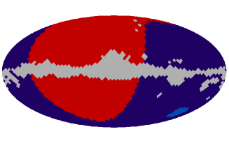
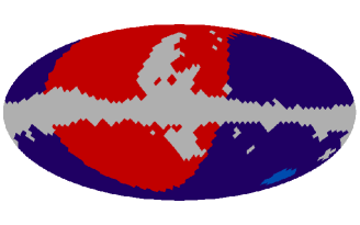
Figure 1: Mollweide projection of the observed Northern (red) and Southern (blue) hemisphere at $N_{\rm side}=16$. The (light blue) circle in the Southern hemisphere corresponds to the region of the Cold Spot, whereas the light grey region corresponds to the WMAP low resolution galactic mask for temperature (upper panel) and polarization (lower panel).

To assess the significance of the power asymmetries found in the data, our results have been tested against Monte Carlo simulations. A set of 1000 CMB+noise sky realizations has been generated: the signal was generated from the WMAP 5 year best fit model, the noise through a Cholesky decomposition of the global ($T,Q,U$) noise covariance matrix. We then computed the angular power spectra for each of the 1000 simulations using BolPol and built two figures of merit as explained in the next subsection.

2.3 Estimators

We define the following quantities

$$C^{X}_{N/S}\equiv{1\over{(\ell_{max}-1)}}\,\sum_{\ell=2,\ell_{max}}{\ell(\ell+1)\over{2\pi}}\,\hat{C}^{X,N/S}_{\ell}$$ (6)

where $\hat{C}^{X,N}_{\ell}$ and $\hat{C}^{X,S}_{\ell}$ are the estimated angular power spectra obtained with BolPol observing only the Northern (‘$N$’) and the Southern (‘$S$’) hemisphere respectively, outside the galactic plane. As above, $X$ runs over the spectral types.

Two estimators can be built as follows: the ratio $R^{X}$, as performed in Eriksen et al. (2004),

$$R^{X}=C^{X}_{S}/C^{X}_{N}\,,$$ (7)

and the difference $D^{X}$,

$$D^{X}=C^{X}_{S}-C^{X}_{N}\,,$$ (8)

of the two aforementioned quantities. In the following, we will drop the index $X$ for $R$ and $D$ specifying only the spectrum we refer to.

For our application to WMAP data, both estimators have been considered for $TT$, while only the $D$ estimator has been applied to the other spectra ($EE$, $TE$, $BB$, $TB$ and $EB$), because of unfavorable signal-to-noise ratio of the WMAP data in polarization.

3 Results

The six angular power spectra $TT$, $EE$, $TE$, $BB$, $TB$, $EB$ are presented in Fig. 2 and 3. Our results for $TT$, shown in the upper panel of Fig. 2, are consistent with those obtained by Eriksen et al. (2004).

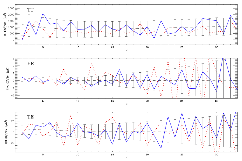
Figure 2: QML estimates for $TT$ (upper panel), $EE$ (middle panel) and $TE$ (lower panel) from WMAP 5 year $N_{\rm side}=16$ maps. Solid (blue) line is for the angular power spectrum of the Southern hemisphere (blue region of Fig. 1), whereas dotted (red) line is for the Northern one (red region of Fig. 1). Dashed line shows the WMAP 5 year best fit, taken as fiducial power spectrum for the analysis. For reference, we also show the error bars of the QML computed from a Monte Carlo of 1000 sky realizations of the Northern hemisphere with the global ($T$,$Q$,$U$) noise covariance matrix (error bars from the Monte Carlo on the Southern hemisphere are basically undistinguishable from the ones plotted).

Figure 3: As in Fig. 2 but for $BB$, $TB$, $EB$ (from top to bottom)

In Fig. 4 we show the $R$ estimator distribution for the range $\ell=2-40$. For this estimator we obtain that the probability of having the WMAP value is as low as $0.2\%$, which agrees with the results by Eriksen et al. (2004). In Table 1 the probability of obtaining the WMAP value for the $D$ estimator is computed for the following four multipoles ranges: $2-8$, $2-16$, $2-32$ and $2-40$. See Fig. 5 for the full empirical (Monte Carlo) probability distribution functions. Note that the $R$ and $D$ estimator detect a comparable level of anomaly in the multipole range $2-40$.

In Table 2 we provide results for polarization and cross-spectra. As mentioned above, only $D$ is considered and computed for the four aforementioned multipoles range. The estimator $R$, in fact, is not well defined any time the denominator $C_{N}^{X}$ approaches to zero, which might be the case for highly noisy spectra. Although Table 2 does not show any significant deviation from the symmetry for polarization and cross-spectra, it is nonetheless worth noting the behaviour of $EE$ in the range $\ell=2-16$, for which the probability of having the WMAP value is as low as $3.5\%$, and of $BB$ in the range $\ell=2-8$ where the probability decreases to $2.2\%$. Moreover, an unexpected statistics seems to show up for $TE$ in the range $2-40$ where the probability of having the WMAP value is $0.5\%$. However, this mainly comes from the multipoles between $32$ and $40$, which are close to the threshold of reliability of the QML on $N_{\rm side}=16$ maps.

Table 1: Probabilities (in percentage) to obtain a smaller value than WMAP low resolution data for $TT$ angular power spectrum and the $D$-estimator.

$D$	$\Delta\ell$ = 2-8	$\Delta\ell$ = 2-16	$\Delta\ell$ = 2-32	$\Delta\ell$ = 2-40
$TT$	86.2	96.9	99.8	99.1

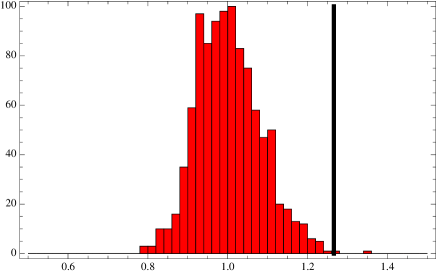
Figure 4: $TT$. Number counts ($y$-axis) versus $R$ ($x$-axis) for the range $\Delta\ell=[2,40]$. The vertical line stands for the WMAP 5 yr data. The probability to obtain a smaller value than the WMAP one is $99.8\%$.

Table 2: Probabilities (in percentage) to obtain a smaller value than WMAP low resolution data

$D$	$\Delta\ell$ = 2-8	$\Delta\ell$ = 2-16	$\Delta\ell$ = 2-32	$\Delta\ell$ = 2-40
$TE$	59.9	16.9	75.6	99.5
$EE$	5.4	3.5	28.8	34.3
$BB$	97.8	79.5	71.9	81.0
$TB$	80.9	54.1	42.8	91.7
$EB$	61.3	54.6	74.4	21.8

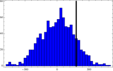
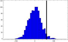
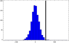
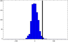
Figure 5: $TT$. All the panels present the number counts ($y$-axis) versus the $D$ statistics ($x$-axis), being the latter in units of $\mu K^{2}$. For each panel, $D$ has been computed within a different range of multipoles. Top left: $\Delta\ell=[2,8]$. Top right: $\Delta\ell=[2,16]$. Bottom left: $\Delta\ell=[2,32]$. Bottom right: $\Delta\ell=[2,40]$. Vertical lines for the WMAP 5 yr data.

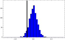
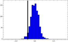
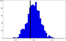
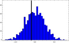
Figure 6: As in Fig. 5 but for $EE$.

We also report on the possible contribution to the North-South power asymmetry given by the Cold Spot found by Vielva et al. (2004) (see also Cruz et al. (2005, 2007)). By masking out the Cold Spot (see light blue spot of Fig. 1) with a circle of radius 8 degrees - a conservative choice compared to its size of 5 degrees - we have not found any significant deviation from the $C_{\ell}$ obtained without masking it out. This might be due to the fact that the low resolution of our data set prevents us from exploring properly the angular scales of interest for the physical size of the Cold Spot ($\ell\simeq 40$). Moreover, the smoothing process applied to the temperature map might be also responsible for washing out features like the Cold Spot. Nonetheless, a possible connection between these large scale anomalies has been claimed recently in Bernui (2009), where a different estimator with respect to the one adopted in the present analysis has been exploited. Withstanding all the caveats set forth above, our analysis suggests that the Cold Spot has little to do with WMAP 5 year asymmetries.

4 Planck Forecasts

The Planck satellite (The Planck Collaboration, 2006) has been launched on May 14th, 2009, and it will measure CMB anisotropies with unprecedented precision. In order to assess its capabilities in probing the hemispherical asymmetry, we consider the nominal sensitivity of the Planck 143 GHz channel, taken as representative of the results which can be obtained after the foreground cleaning from various frequency channels. The 143 GHZ channel has an angular resolution of $7.1^{\prime}$ (FWHM) and an average sensitivity of $6\mu K$ ($11.4\mu K$) per pixel - a square whose side is the FWHM size of the beam - in temperature (polarization), after 2 full sky surveys (The Planck Collaboration, 2006). We assume uniform uncorrelated instrumental noise and we build the corresponding diagonal covariance matrix for temperature and polarization, from which, through Cholesky decomposition we are able to extract noise realizations.

As expected, we notice that no significant improvement will be achieved with Planck for the $TT$ spectrum, since both WMAP and Planck are cosmic variance limited for the range of multipoles considered here. On the contrary, polarization and cross-spectra do benefit from the Planck increased sensitivity. In Fig. 13 we plotted our forecasted distribution for the estimator $D$ for $TE$ and $EE$ on top of the same distribution for the WMAP case: the shrinking of the distribution due to the higher sensitivity is more than evident. Moreover, for these two cases we find that also the $R$ estimator yields valuable information. Finally, we do not expect to be able to apply the $R$ estimator for any spectrum involving $B$ because of the low level of signal, if any. Distributions of $D$ for $BB$, $TB$ and $EB$ are analogous to what shown for $TE$ and $EE$.

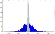
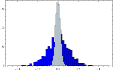
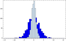
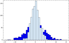
Figure 7: Comparison between WMAP and Planck for $EE$ (upper panels) and for TE (lower panels). Left panels: number counts for $D$ with $\Delta\ell=[2,16]$. Right panels: $D$ with $\Delta\ell=[2,8]$. In all the panels, dark blue is for WMAP and light blue is for Planck. Units for $D$ in the $x$-axis are $\mu K^{2}$.

5 Discussions and Conclusions

Using an optimal power spectrum estimator, we have confirmed the power asymmetry for $TT$ found by Eriksen et al. (2004) along the direction reported in Hansen et al. (2009), see Table 1 and Fig. 5. Considering the same axis, we have extended such analysis to the other spectra ($TE$, $EE$, $BB$, $TB$ and $EB$) considering only the estimator $D$, defined in Eq. (8), because the noise level of WMAP permits the use of R (see Eq. (7)) only for $TT$.

Since our implementation of the QML (Gruppuso et al., 2009) is capable of handling the full noise covariance matrix in ($T$,$Q$,$U$), the analysis of the present paper is joint for temperature and polarization. The information encoded in CMB polarization is complementary to the temperature and is important to test for possible asymmetries in polarization (see for instance Dvorkin, Peiris and Hu (2008) for the description of the polarization field in models that break statistical isotropy locally through a modulation field). We confirm the $TT$ anomalies that have been already reported by severals groups. Our analysis of polarized and cross-spectra does not show significant anomalies, as from Table 2.

The origin of the these hemispherical asymmetries is still unknown. They can be primordial or due to some residual foreground or systematic effect. For instance, in Li et al. (2009) an anomalous correlation between temperature and observation number has been claimed to be present in the WMAP 5yr data, potentially impacting the large scale pattern of CMB maps (including the power asymmetries). In that paper, this effect has been related to an imbalance in the differential observation scheme of the WMAP mission. Planck is observing the sky with a totally different scheme and therefore is free from this particular systematic effect.

Planck will be able to furtherly confirm the temperature anomalies and shed new light onto the polarization sector: the quality of Planck data (The Planck Collaboration, 2006; Bersanelli et al., 2010; Mandolesi et al., 2010; Mennella et al., 2010) is expected to be sufficiently high to use the $R$ estimator even for polarization and cross spectra. We show the improvements for the $D$ estimator expected from Planck in Fig. 7.

No significant differences have been found by masking the Cold Spot in the Southern hemisphere with a disk of $8$ degrees of radius (conservative choice). Despite of the possible causes we mentioned in Section 3, we think that our results in this respect is worthy of note. Further investigation is needed since a correlation between these two anomalies (i.e. the Cold Spot and the North-South asymmetry) has been recently claimed (Bernui, 2009), especially in the polarization sector where the properties of the Cold Spot are still unclear (Vielva et al., 2010).

References

- Bernui (2009) Bernui A., Phys. Rev. D 80, 123010 (2009)
- Bersanelli et al. (2010) Bersanelli, M., et al. 2010, arXiv:1001.3321
- Bunn et al. (2003) Bunn E. F., Zaldarriaga M., Tegmark M. and de Oliveira-Costa A., Phys. Rev. D 67 (2003) 023501
- Cruz et al. (2005) Cruz, M., Martínez-González, E., Vielva, P., & Cayón, L. 2005, Mon Not. Roy. Astron. Soc, 356, 29
- Cruz et al. (2007) Cruz, M., Cayón, L., Martínez-González, E., Vielva, P., & Jin, J. 2007, Astrophys. J., 655, 11
- Dunkley et al. (2009) Dunkley J. et al. [WMAP Collaboration], Astrophys. J. Suppl. 180 (2009) 306
- Dvorkin, Peiris and Hu (2008) Dvorkin C., Peiris H. V. and Hu W., Phys. Rev. D 77 (2008) 063008
- Eriksen et al. (2004) Eriksen H.K., Hansen F.K., Banday A.J., Gorski K.M. and Lilje P.B., Astrophys. J. 605 (2004) 14 [Erratum-ibid. 609 (2004) 1198]
- Eriksen et al. (2007) Eriksen H.K., Banday A.J., Gorski K.M., Hansen F.K. and Lilje P.B., Astrophys. J. 660 (2007) L81
- Gorski et al. (2005) Gorski K.M., Hivon E., Banday A.J., Wandelt B.D., Hansen F.K., Reinecke M. and Bartelmann M., 2005, Astrophys. J., 622, 759-771
- Gruppuso et al. (2009) Gruppuso A., De Rosa A., Cabella, P., Paci F., Finelli F., Natoli P., de Gasperis G. and Mandolesi N., Mon. Not. Roy. Astron. Soc. 400 (2009) 463
- Hansen et al. (2004) Hansen F. K., Banday A. J. and Gorski K. M., Mon. Not. Roy. Astron. Soc. 354 (2004) 641
- Hansen et al. (2009) Hansen F. K., Banday A. J., Gorski K. M., Eriksen H. K. and Lilje P. B., Astrophys. J. 704 (2009) 1448
- Hinshaw et al. (2009) Hinshaw, G. et al. [WMAP Collaboration], Astrophys. J. Suppl. 180 (2009) 225
- Hoftuft et al. (2009) Hoftuft J., Eriksen H. K., Banday A. J., Gorski K. M., Hansen F. K. and Lilje P. B., Astrophys. J. 699 (2009) 985
- Li et al. (2009) Li T. P., Liu H., Song L. M., Xiong S. L. and Nie J. Y., arXiv:0905.0075 [astro-ph.CO].
- Mandolesi et al. (2010) Mandolesi, N., et al. 2010, arXiv:1001.2657
- Mennella et al. (2010) Mennella, A., et al. 2010, arXiv:1001.4562
- The Planck Collaboration (2006) The Planck Collaboration, “The Scientific Programme of Planck” arXiv:astro-ph/0604069.
- Smith and Zaldarriaga (2009) Smith K. M. and Zaldarriaga M., Phys. Rev. D 76 (2007) 043001
- Tegmark (1997) Tegmark M., Phys. Rev. D 55, 5895 (1997)
- Tegmark and de Oliveira-Costa (2001) Tegmark M. and de Oliveira-Costa A., Phys. Rev. D 64 (2001) 063001
- Vielva et al. (2004) Vielva, P., Martínez-González, E., Barreiro, R. B., Sanz, J. L., & Cayón, L. 2004, Astrophys. J, 609, 22
- Vielva et al. (2010) Vielva, P., Martinez-Gonzalez, E., Cruz, M., Barreiro, R. B., & Tucci, M. 2010, arXiv:1002.4029