Entanglement detection from interference fringes in atom-photon systems

Abstract

A measurement scheme of atomic qubits pinned at given positions is studied by analyzing the interference pattern obtained when they emit photons spontaneously. In the case of two qubits, a well-known relation is revisited in which the interference visibility is equal to the concurrence of the state in the infinite spatial separation limit of the qubits. By taking into account the superradiant and subradiant effects, it is shown that a state tomography is possible when the qubit spatial separation is comparable to the wavelength of the atomic transition. In the case of three qubits, the relations between various entanglement measures and the interference visibility are studied, where the visibility is defined from the two-qubit case. A qualitative correspondence among these entanglement relations is discussed. In particular, it is shown that the interference visibility is directly related to the maximal bipartite negativity.

I Introduction

Much attention has been raised recently to the study of atom-photon systems, such as ultracold atoms and trapped ions, in view of quantum information and computation processing protocols Rev . Achieving these protocols with hybrid systems requires the capability of manipulating atoms and photons with high precision as well as long coherence time for qubits. As an example of such demands, an ability to prepare highly entangled states is needed in the beginning of protocols. It is then necessary to verify the quality of these entangled states and this can be accomplished by performing a quantum state tomography PR . However, it is rather difficult to perform the full tomography, in general, and it becomes impractical as the size of Hilbert space increases. An alternative to the quantum state tomography is to perform a set of measurements to detect the amount of entanglement in the state. It is the main objective of this paper to investigate a passive measurement scheme for entanglement detection by analyzing the interference pattern of photons emitted by atoms.

Since entanglement and correlation are closely related to each other, a relationship between the interference visibility and entanglement in bipartite systems has been anticipated in the context of wave-particle duality JSV ; EB . Jacob and Bergou observed that two-qubit concurrence is equivalent to two-particle interference visibility in the case of pure states JB03 . To be self-contained, let us consider a simplified argument for the known correspondence between the visibility and the concurrence by the detection of released photons in the far-field JSV ; JB03 . Consider two two-level atoms in which energy levels are $|e\rangle$ and $|g\rangle$, respectively. Assume an initial atomic state living in the subspace spanned by $|0\rangle=|eg\rangle$ and $|1\rangle=|ge\rangle$,

$$\rho=\left(\begin{array}[]{cc}|0\rangle,|1\rangle\end{array}\right)\left(\begin{array}[]{cc}\rho_{00}&\rho_{01}\\ \rho_{10}&\rho_{11}\end{array}\right)\left(\begin{array}[]{c}\langle 0|\\ \langle 1|\end{array}\right)\,,$$ (1)

whose concurrence is $C(\rho)=2|\rho_{01}|$. The spontaneous emission process of a single photon (i.e., $\rho\to|gg\bm{k}\rangle$) occurs with equal probability but different phases. Ignoring the details of the coupling between the atoms and the radiation field, the standard Michelson’s visibility is defined by

$${\cal V}(\rho)=\frac{I_{{\rm max}}-I_{{\rm min}}}{I_{{\rm max}}+I_{{\rm min}}}\,,$$ (2)

where $I_{{\rm max}}=\max_{0\leq\Phi<2\pi}\mathop{\mathrm{Tr}}(I(\Phi)\rho)$ and $I_{{\rm min}}=\min_{0\leq\Phi<2\pi}\mathop{\mathrm{Tr}}(I(\Phi)\rho)$ are the maximum and the minimum of interference fringes, respectively, and the projection measurement of the phase $\Phi$ is given by $I(\Phi)=|\Phi\rangle\langle\Phi|$ with $|\Phi\rangle=(|0\rangle+\,\mathrm{e}^{\mbox{\footnotesize$\mathrm{i}\Phi$}}|1\rangle)/\sqrt{2}$. It is straightforward to evaluate the visibility in this model as

$${\cal V}(\rho)=2|\rho_{01}|=C(\rho)\,,$$ (3)

and this completes the claim comment2 . We emphasize that visibility here is not the two-particle visibility defined from a combination of correlation functions, which is shown to be equivalent to the concurrence of the pure state spanned by $|gg\rangle,|eg\rangle,|ge\rangle,|ee\rangle$ JSV ; JB03 .

Several generalizations addressing the case of mixed states, of two qudits, and of multipartite qubits have also been reported recently Durr ; Tessier ; HCO ; JB07 ; EKKC . Despite these progresses, there is still no net conclusive result on general multipartite systems. This is simply due to the fact that no generally accepted entanglement measure and no unique definition of interference visibility exist in multipartite systems. The former, for example, can be seen from the fact that none of these existing measures can be used to order the entangled states uniquely EP ; WNGKMV ; VADM . The latter problem was addressed in Ref. EKKC where a systematic construction for the visibility and the so-called predictability were introduced starting from minimal requirements for a proper definition of these concepts.

In this paper, we analyze the interference pattern generated by photons spontaneously emitted by a set of two-level atoms and we investigate the relation between entanglement and interference visibility. To explore various kinds of two-qubit and three-qubit entangled states, we consider identical two-level atoms pinned at given positions and initially prepared in a superposition of the first excited states of the atoms. In the course of time, a photon is later released from the excited atom in any direction. In our setting, quantum statistical effects play no role and complications related to the atomic motion, such as Doppler and recoil effects, are avoided. In an experimental situation, this would be realized, for example, with atoms trapped in different potential wells in the Lamb-Dicke regime.

Another motivation of this work is to clarify the meaning of the standard interference visibility (2) defined in two-path interferometers when it is applied to three-path interferometers. In Ref. EKKC for example, it was shown that there is an infinite family of state functions which could be considered as equally good measures of the interference strength. In the present paper, however, rather than studying these many other alternatives, the usual standard definition (2) is employed to examine what one can learn from it.

The content of this paper is as follows. Section II provides a brief summary for the known results on two two-level atoms interacting with the radiation field. In Sec. III the interference pattern is analyzed when the emitted photon is detected in the far-field and is compared with the entanglement present in the initial (possibly mixed) state. It is confirmed that the interference visibility converges to the concurrence when the spatial separation of the qubits goes to infinity. In Sec. III C, a state tomography is shown to be possible when the separation between the qubits is on the order of the wavelength of the atomic transition. In Sec. IV the previous analysis is extended when the initial atomic qubit state is pre- pared in a W-like pure state. The relationship is studied between the interference visibility and known entanglement measures. In particular, the interference visibility is shown to be able to detect bipartite entanglement. A brief discussion is given in Sec. IV D on a state tomography for the W-like state. A summary and possible extensions of the work are stated in Sec. V. The Appendix contains the definitions of the entanglement measures used in the paper.

II Superradiance and Subradiance from radiative corrections

We briefly review some known results for two atoms interacting with the quantized radiation field. A more detailed account can be found in Ref. CT .

Consider two neutral two-level atoms which are pinned at given positions $\bm{x}_{j}$ ($j=1,2$). The internal structure of each isolated atom consists of a unique excited state $|e\rangle$ at energy $\hbar\omega_{e}$ with radiative lifetime $\tau=1/\Gamma$, which is separated by the energy $\hbar\omega_{0}=\hbar ck_{0}=2\pi\hbar c/\lambda_{0}$ from a unique ground state $|g\rangle$ at energy $\hbar\omega_{g}$. Throughout the paper, a simple scalar model for the atom-field interaction is considered and any polarization effects are neglected. Fixing the origin of energy at the ground-state levels (i.e., at $2\hbar\omega_{g}$) the free atoms-field Hamiltonian $H_{0}$ for this case reads

$$H_{0}=\sum_{j=1,2}\hbar\omega_{0}\ |e_{j}\rangle\langle e_{j}|+\sum_{\bm{k}}\hbar\omega a^{\dagger}_{\bm{k}}a_{\bm{k}}\,,$$ (4)

where $a_{\bm{k}}$ and $a^{\dagger}_{\bm{k}}$ stand for the annihilation and creation operators of a photon with momentum $\bm{k}$ and angular frequency $\omega=c|\bm{k}|$. The total Hamiltonian is $H=H_{0}+V$, where the coupling of atoms to the radiation field is given by

$$V=-\sum_{j=1,2}d_{j}E(\bm{x}_{j})\,,$$ (5)

in the dipole approximation. Here the scalar radiation field $E(\bm{x})$ reads

$$E(\bm{x})=\mathrm{i}\sum_{\bm{k}}{\cal E}_{\omega}\left(\,\mathrm{e}^{\mbox{\footnotesize$\mathrm{i}\bm{k}\cdot\!\bm{x}$}}a_{\bm{k}}-\,\mathrm{e}^{\mbox{\footnotesize$-\mathrm{i}\bm{k}\cdot\!\bm{x}$}}a^{\dagger}_{\bm{k}}\right)\,,$$ (6)

where ${\cal E}_{\omega}=\sqrt{\hbar\omega/(2\epsilon_{0}L^{3})}$ is the field strength at energy $\hbar\omega$ and $L$ is the size of the quantization box used to define the photon modes. The dipole operator for the $j$th atom is

$$d_{j}=d\ (|e_{j}\rangle\langle g_{j}|+|g_{j}\rangle\langle e_{j}|)\,.$$ (7)

Within the scalar radiation model, the dipole strength $d$ relates to the radiative width of the excited state through $\Gamma=d^{2}k_{0}^{3}/(2\pi\hbar\epsilon_{0})$. In the following, when there is no possible ambiguity for labeling the internal atomic states, the atomic index $j$ is omitted.

Consider the situation where at time $t=0$ the radiation field is in its vacuum state $|\bm{0}\rangle$, while one of the atomic qubits is in the excited state. In other words the system starts in the subspace ${\cal H}_{P}$ spanned by the first excited states without photons (i.e., $|eg\bm{0}\rangle$ and $|ge\bm{0}\rangle$). Because these first excited states are coupled to the radiation field, they eventually decay to the atomic ground state $|gg\rangle$ by releasing a spontaneous photon $|\bm{k}\rangle$. This process can be described by the method of the resolvent operator $G(z)=(z-H)^{-1}$ and its projection on the various subspaces of interest CT . For example, the time-evolution operator restricted to the subspace ${\cal H}_{P}$ is obtained from a contour integral of the following projected resolvent operator

$$G_{P}(z)={\cal P}\frac{1}{z-H_{0}-V}{\cal P}\,,$$ (8)

$${\cal P}=|eg\bm{0}\rangle\langle eg\bm{0}|+|ge\bm{0}\rangle\langle ge\bm{0}|\,,$$ (9)

where ${\cal P}$ is the projector onto the subspace ${\cal H}_{P}$. To second order in the coupling constant, its diagonalized form reads

$$G_{P}(z)\simeq|+\rangle\frac{1}{z-\hbar\Omega_{+}}\langle+|+|-\rangle\frac{1}{z-\hbar\Omega_{-}}\langle-|\,,$$ (10)

where the corresponding eigenkets $|\pm\rangle$ are given by

$$|\pm\rangle=\frac{1}{\sqrt{2}}(|eg\bm{0}\rangle\pm|ge\bm{0}\rangle)\,,$$ (11)

and the complex eigenvalues $\Omega_{\pm}=\omega_{\pm}-\mathrm{i}\Gamma_{\pm}/2$ are comment5

$$\omega_{\pm}=\omega_{0}\mp\frac{\Gamma}{2}g(k_{0}r)\,,$$ (12)

$$\Gamma_{\pm}=\Gamma\left[1\pm f(k_{0}r)\right]\,,$$ (13)

$$g(x)=\cos(x)/x,\ f(x)=\sin(x)/x\,,$$ (14)

where $r=|\bm{x}_{1}-\bm{x}_{2}|$ is the distance between the atoms.

The net effect of the interaction with the radiation field is to lift the degeneracy between the initial atomic states in the subspace ${\cal H}_{P}$. The physical process behind it is the resonant exchange of photons between the atoms which “glues” the atoms together and gives rise to the states $|\pm\rangle$ in a fashion similar to the bonding and antibonding states of a molecule. The new levels also acquire different finite lifetimes. The subspace ${\cal H}_{P}$ is thus irreversibly emptied by spontaneous emission in the course of time while the ground state is gradually populated. Both the degeneracy splitting and the lifetimes depend on the relative distance $r$ between the atoms. For sufficiently close atoms, the celebrated superradiant and subradiant behaviors are recovered in which the eigenstates are given by $|+\rangle$ and $|-\rangle$, respectively. The atomic dipoles are perfectly correlated (i.e., they oscillate in phase for the superradiant state and in phase opposition for the subradiant state). For $|+\rangle$, the radiation waves emitted by the two atoms interfere constructively and the system radiates more efficiently, shortening its lifetime. For $|-\rangle$, on the other hand, the waves interfere destructively and the system cannot radiate, increasing its lifetime. Indeed one gets $\Gamma_{+}\to 2\Gamma$ and $\Gamma_{-}\to 0$ in the limit $k_{0}r\to 0$ CT .

In the other extreme limit $k_{0}r\to\infty$, both lifetimes achieve the value obtained for a single isolated atom $\Gamma_{\pm}\to\Gamma$. In this limit the atoms are no longer coupled by the radiation field, and the energy degeneracy in the subspace ${\cal H}_{P}$ shows up again $\omega_{\pm}\to\omega_{0}$.

The time evolution of the initial state decaying into the ground state is obtained from a contour integral of another projected resolvent

$$G_{QP}(z)={\cal Q}\frac{1}{z-H_{0}-V}{\cal P},\quad{\cal Q}=1-{\cal P}\,.$$ (15)

The matrix elements of $G_{QP}(z)$ read

$$\langle gg\bm{k}|G_{QP}(z)|\pm\rangle\simeq\frac{\mathrm{i}\hbar g_{\omega}}{\sqrt{2}}\ \frac{\,\mathrm{e}^{\mbox{\footnotesize$-\mathrm{i}\bm{k}\cdot\!\bm{x}_{1}$}}\pm\,\mathrm{e}^{\mbox{\footnotesize$-\mathrm{i}\bm{k}\cdot\!\bm{x}_{2}$}}}{(z-\hbar\omega)(z-\hbar\Omega_{\pm})}\,,$$ (16)

where $g_{\omega}=d{\cal E}_{\omega}/\hbar$ is the Rabi frequency at field angular frequency $\omega$. One can easily check that $\langle gg\bm{k}|G_{QP}(z)|-\rangle\to 0$ when $k_{0}r\to 0$ as expected for the subradiant state since it does not couple anymore to the radiation field in this limit.

III Entanglement detection: The case of two atoms

III.1 Visibility in the infinite separation limit

Let us now proceed to verify the result (3) based on the microscopic model presented in the previous section. As before, consider the initial state (1) of atoms within the subspace spanned by $|ge\bm{0}\rangle$ and $|eg\bm{0}\rangle$, and parametrize the density matrix as

$$\rho_{2}=(|eg\bm{0}\rangle,\ |ge\bm{0}\rangle)\frac{1}{2}\left(\begin{array}[]{cc}1\!+\!s_{z}&s_{x}\!-\!\mathrm{i}s_{y}\\ s_{x}\!+\!\mathrm{i}s_{y}&1\!-\!s_{z}\end{array}\right)\binom{\langle eg\bm{0}|}{\langle ge\bm{0}|}\,,$$ (17)

where $s_{x}=s\sin\theta\cos\phi$, $s_{y}=s\sin\theta\sin\phi$, and $s_{z}=s\cos\theta$ are the components of the vector $\bm{s}$ with the ranges $0\leq\theta\leq\pi$, $0\leq\phi\leq 2\pi$, and $0\leq s\leq 1$. The concurrence of the state (17) is $C(\rho_{2})=s\sin\theta$.

In the model considered, the interference visibility (2) is defined by the maximum and the minimum values achieved by the spectral distribution of the spontaneous photon over all possible emission directions. This spectral distribution is proportional to the transition probability $P(\rho_{2}\to|gg\bm{k}\rangle)$ from the initial state (17) to the ground state $|gg\bm{k}\rangle$. This is obtained from the time evolution of the state $\rho_{2}(t)=U(t)\rho_{2}U^{\dagger}(t)$ in the long-time limit $\Gamma t\to\infty$ where $U(t)$ is the time-evolution unitary operator calculated from (16) as follows:

$$P(\rho_{2}\to|gg\bm{k}\rangle)=\lim_{\Gamma t\to\infty}\mathop{\mathrm{Tr}}\left(|gg\bm{k}\rangle\langle gg\bm{k}|\rho_{2}(t)\right)$$ (18)

$$=\!\frac{\Gamma\omega}{(2\pi)^{2}k_{0}^{3}}\left[\frac{{\cal B}_{+}}{(\omega\!-\!\omega_{+})^{2}\!+\!(\Gamma_{+}/2)^{2}}\!+\!\frac{{\cal B}_{-}}{(\omega\!-\!\omega_{-})^{2}\!+\!(\Gamma_{-}/2)^{2}}\right],$$

where the coefficients ${\cal B}_{\pm}$ are

$${\cal B}_{\pm}\!=\!\frac{1}{4}\left[(1\pm s_{x})(1\pm\cos\bm{k}\!\cdot\!\bm{r})\!+\!\frac{1\!\pm\!f}{1\!+\!g^{2}}(s_{y}-gs_{z})\sin\bm{k}\!\cdot\!\bm{r}\right],$$

with the shorthands $f\equiv f(k_{0}r)$ and $g\equiv g(k_{0}r)$, and $\bm{r}=\bm{x}_{1}-\bm{x}_{2}$ is the relative vector connecting the two atoms. In Eq. (18), the spectral distribution is a weighted sum of two Lorentzians centered at angular frequencies $\omega_{\pm}$ with respective widths $\Gamma_{\pm}$. The angular frequency separation $\Delta\omega=|\omega_{+}-\omega_{-}|$ between the two peaks is generally small and the atoms need to be located rather close to each other to distinguish them. This can be seen from the ratio

$$\frac{\Delta\omega}{\Gamma_{\pm}}=\left|\frac{g(k_{0}r)}{1\pm f(k_{0}r)}\right|\,,$$ (19)

which is a small number when atoms are located far apart compared with the optical atomic transition wavelength.

To extract the visibility of the interference pattern, the distribution (18) is to be maximized and minimized over the spherical angles of the emitted photon. Rewrite (18) as

$$P(\rho_{2}\!\to\!|gg\bm{k}\rangle)\!=\!\frac{\Gamma\omega}{(2\pi)^{2}k_{0}^{3}}\left[\xi_{+}\!+\!\sqrt{\xi_{-}^{2}\!+\!\eta^{2}}\cos(\bm{k}\!\cdot\!\bm{r}-\theta_{0})\right],$$ (20)

with the notations

$$\xi_{\pm}\!=\!\frac{1+s_{x}}{(\omega\!-\!\omega_{+})^{2}\!+\!(\Gamma_{+}/2)^{2}}\pm\frac{1-s_{x}}{(\omega\!-\!\omega_{-})^{2}\!+\!(\Gamma_{-}/2)^{2}}\,,$$ (21)

$$\eta\!=\!\left[\frac{1+f}{(\omega\!-\!\omega_{+})^{2}\!+\!(\Gamma_{+}/2)^{2}}+\frac{1-f}{(\omega\!-\!\omega_{-})^{2}\!+\!(\Gamma_{-}/2)^{2}}\right]$$

$$\hskip 156.49014pt\times\frac{s_{y}-gs_{z}}{1+g^{2}}\,,$$ (22)

and $\theta_{0}=\tan^{-1}(\eta/\xi_{-})$. It is clear that the maxima and minima occur when $\cos(\bm{k}\!\cdot\!\bm{r}-\theta_{0})=\pm 1$. The far-field fringe visibility is thus

$${\cal V}(r,\omega;\rho_{2})=\frac{\sqrt{\xi_{-}^{2}+\eta^{2}}}{\xi_{+}}\,.$$ (23)

It is straightforward to calculate the visibility in the infinite separation limit as

$$\lim_{r\to\infty}{\cal V}(\omega,r;\rho_{2})=\sqrt{s_{x}^{2}+s_{y}^{2}}=s\sin\theta=C(\rho_{2})\,.$$ (24)

Therefore, the result (3) is valid only in the infinite separation limit. From a practical point of view, the infinite separation limit is reached as soon as the two atoms are separated by a large distance compared to the wavelength $\lambda_{0}$ of the optical transition of each individual atom.

A full characterization of the initial state $\rho_{2}$ is completed as soon as the full vector $\bm{s}$ associated to $\rho_{2}$ is known, see (17). Note that the angle $\theta_{0}$ describes a shift of the interference pattern perpendicular to the plane located at equal distances from the atoms and that it converges to the angle $\phi$ in the limit $r\to\infty$. Thus, knowing the positions $\bm{x}_{j}$ of the atoms, the pattern shift can be measured in principle and $\phi$ can be extracted from the data. From the visibility and the interference pattern shift, $s_{x}$ and $s_{y}$ can be obtained. However one still needs to extract the missing component $s_{z}$ from the data, which is unfortunately not possible in the infinite separation limit. Complete state tomography is studied in Sec. III C. As a last remark, the angular separation between two consecutive fringes is inversely proportional to distance $r$. This means that the further apart atoms are located, the more periodic and regular the fringe pattern appears. Therefore, by knowing the distance between the two atoms, one does not need to measure the whole interference pattern for all angular positions. It is sufficient to record a few fringes to detect the amount of entanglement.

III.2 Interference visibility for finite distances

In this section, we analyze the deviation ${\cal V}(r,\omega;\rho_{2})-C(\rho_{2})$ of the interference visibility obtained for atoms at finite distances, Eq. (23), from its asymptotic value obtained for atoms far apart, that is, from the concurrence $C(\rho_{2})=s\sin\theta$ of the two-qubit initial state. Our interest is in the state and distance dependency of this deviation and particularly in the maximal possible deviation from the concurrence for a given distance $r$ between the atoms. The latter number can be used as a quantitative measure for the relationship between interference visibility and entanglement when estimating the amount of entanglement in the initial state from the observed visibility.

First, from the result (23) it can be seen that the deviation can be both positive and negative, and converges to zero in the limit $r\to\infty$ as was shown in (24). Next, we numerically calculate the maximal value reached by $|{\cal V}-C|$ as a function of $r$ (in units of $\lambda_{0}$) for some specific values of the state purity $s=1.0,0.5,0.1$. To this end, the deviation $|{\cal V}-C|$ is maximized over the state parameters $\theta$, $\phi$ at fixed $r$ and $s$. The frequency of the emitted photon is set at $\omega_{0}$. This can be achieved, for example, by frequency filtering in the detection process. Without such filtering, one would have to integrate over all range of frequencies in Eq. (18) to get the observed fringes. The result, depicted in Fig. 1, shows an oscillatory decay of $\max_{\theta,\phi}|{\cal V}-C|$ when $r$ is increased. The local minima occur when $k_{0}r$ is an integer multiple of $\pi$, that is, when $f(k_{0}r)=0$. For these particular atomic separations, the superradiant and subradiant states have exactly the same decay rate $\Gamma_{\pm}=\Gamma$ but still different eigenfrequencies. The local maxima occur when $k_{0}r\pm\pi/2$ is a multiple integer of $2\pi$, that is, when $g(k_{0}r)=0$. In this case, the superradiant and subradiant states have identical eigenfrequencies $\omega_{\pm}=\omega_{0}$, but achieve different decay rates. As one can see, the values of the local maxima are insensitive to the purity of the state whereas the values of the local minima increase monotonically when the purity of the state is increased.

Figure 1: Plot of $\max_{\theta,\phi}|{\cal V}-C|$ as a function of $r$ (in units of $\lambda_{0}$) for different values of the purity $s=1.0,0.5,0.1$. The photon angular frequency has been set at $\omega_{0}$. The local minima occur when $f(k_{0}r)=0$ (i.e., when $r$ is a multiple integer of $\lambda_{0}/2$) while the local maxima occur when $g(k_{0}r)=0$ (i.e., when $r$ is an odd multiple integer of $\lambda_{0}/4$). The values achieved by the local maxima are purity independent while the values achieved by the local minima increase with the purity. The solid line represents the analytical result for $s=0$, Eq. (25).

For $s=0$, $C(\rho_{2})=0$ and we get the analytical result

$$|{\cal V}-C|=\frac{2k_{0}r|\sin(k_{0}r)|}{1+(k_{0}r)^{2}}.$$ (25)

It may seem counterintuitive that one gets nonzero fringe visibility when the purity of the initial state is $s=0$ (i.e., when the concurrence of the state is zero and no coherence seems present in the system). In this case, the initial state $\rho_{2}$ describes a complete statistical mixture of the qubit states $|eg\rangle$ and $|ge\rangle$ and one can hardly imagine measuring interference fringes using a Young slit device operating with one slit shut. The reason is that, due to the resonant exchange of photons between the atoms, the radiating eigenstates are not $|eg\bm{0}\rangle$ and $|ge\bm{0}\rangle$ but the superradiant and subradiant states $|\pm\rangle=(|eg\bm{0}\rangle\pm|ge\bm{0}\rangle)/\sqrt{2}$. The initial state at $t=0$ is also equivalent to a complete statistical mixture of $|\pm\rangle$, and both the superradiant and subradiant states display well-defined relative phases between the states $|eg\rangle$ and $|ge\rangle$. Both states $|\pm\rangle$ lead to an interference pattern independently in the far-field, the dark fringes of one pattern corresponding to the bright fringes of the other and vice verse. In addition, these states decay with different rates. Therefore the sum of their respective interference patterns does not average out except in the limit $r\to\infty$. This is easily seen from Eqs. (21) and (III.1) where $\eta=0$ and $\theta_{0}=0$ for $s=0$ and hence the visibility of the interference pattern for $s=0$ relates to the difference of the Lorentzians. For atoms that are far apart, the Lorentzians are essentially identical and cancel out, and the interference is lost. In this limit, the intuitive result is recovered in which the radiation takes place starting from the complete statistical mixture of the qubit states $|eg\rangle$ and $|ge\rangle$. For atoms that are close enough, however interference fringes do occur as the result of the overlap and partial blurring of two independent interference patterns, associated to $|+\rangle$ and $|-\rangle$, with different strengths and fringe locations.

As can be seen from Fig. 1 and Eq. (25), large deviations between ${\cal V}(r,\omega;\rho_{2})$ and $C(\rho_{2})$ appear for small separation of the atoms, typically in the region $r<\lambda_{0}$. However, the deviation can still be significant for atoms far apart as it only decays like $2/k_{0}r$ for large spatial separations. It is straightforward to understand why the argument presented in the Introduction to derive the relation between the visibility and concurrence applies to atoms that are far apart. Concurrence relates to entanglement present in the atomic state $\rho_{2}$ spanned by the states $|eg\rangle$, $|ge\rangle$ irrespective of the coupling to the radiation field while visibility refers to the interference pattern obtained by coupling the atoms to the radiation field (i.e., it relates to the interference pattern obtained from the radiating states $|\pm\rangle$). However, for atoms that are far apart, the resonant exchange of photons between the atoms is negligible and the interaction with the vacuum field does not lift the degeneracy of the subspace ${\cal H}_{P}$. As a consequence, the eigenstructures to analyze radiation and entanglement are then essentially the same. This is why, for atoms that are far apart, the entanglement present in the initial state becomes equivalent to the visibility of the fringes.

III.3 State tomography

In this section, it is shown that, for finite atomic separations, the transition probability $P(\rho_{2}\to|gg\bm{k}\rangle)$ and the visibility ${\cal V}(r,\omega;\rho_{2})$ encode enough information to reconstruct the full initial state (17). This is obvious from Eqs. (18) and (23) which can be directly used to extract the values $s$, $\theta$, and $\phi$ as soon as $r$ is known. Complete knowledge about the initial state then provides information on the amount of entanglement in it.

There are many ways to demonstrate state tomography. For example, consider the simple case where $k_{0}r>1$, but is not too large. The frequency of the emitted photon is set at $\omega_{0}$ as before. Expanding the transition probability and the phase-shift angle up to the first order in $f$ and $g$ reads

$$P(\rho_{2}\to|gg\bm{k}\rangle)\simeq\frac{8c}{(2\pi k_{0})^{2}\Gamma}\ [1\!-\!2fs_{x}$$

$$\hskip 42.67912pt+(s_{x}\!-\!2f)\cos\bm{k}\!\cdot\!\bm{r}+(s_{y}\!-\!gs_{z})\sin\bm{k}\!\cdot\!\bm{r}],$$ (26)

$$\theta_{0}\simeq\tan^{-1}\left(\frac{s_{y}-gs_{z}}{s_{x}}-\frac{2fs_{y}}{s_{x}^{2}}\right)\,.$$ (27)

First of all, knowing $k_{0}r$ calculates the values $f$ and $g$. Second, from the probabilities at $\bm{k}\!\cdot\!\bm{r}=0$ or $\pi$ in Eq. (III.3), the state parameter $s_{x}$ is obtained. Similarly, knowing $s_{x}$ and using the values at $\bm{k}\!\cdot\!\bm{r}=\pm\pi/2$, the combination of state parameters $s_{y}-gs_{z}$ can be found. Last, measuring the approximated phase shift $\theta_{0}$ in Eq. (27) together with the obtained values of $s_{x}$ and $s_{y}-gs_{z}$ provides $s_{y}$ and thus three state parameters $s_{x}$, $s_{y}$, and $s_{z}$. Therefore the full vector $\bm{s}$ is known, completing the state tomography.

The main result of this discussion is that spontaneously emitted photons from the excited states (17) do provide full information about the initial state as well as the amount of entanglement in it. The drawback of this tomographic scheme is that it is not very efficient. Indeed, in the absence of any prior information on the initial state that could help simplify the state search, one needs to measure photons emitted in all directions to obtain the full fringe pattern and later characterize the state. This requires the repeated measurement of photons from an identically prepared state. Although the method is not very practical, it can be combined with other proposals. For example, other possible entanglement detection schemes were studied by many authors. Among them, we mention Ref. SMM , where an entanglement witness was constructed without using the full interference fringe pattern.

IV Interference visibility in the three-atom system

In this section, we extend the previous analysis to the case of three atoms and investigate the relationship between the visibility and the various entanglement measures. This can be accomplished along the same lines of the microscopic calculation done for the two-atom system. As shown in the following, however, a complete analysis appears difficult. Two major obstacles are shown in the following. The full diagonalization of the resolvent operator does not take a simple analytical form except for a few limited cases, for example, when the three atoms are pinned at the vertices of an equilateral triangle. Even for such a special case, finding the extrema of the spectral distribution of photons is unlikely to be carried out by hand, and one needs to rely on numerical calculations in general. It is shown in the following that the large separation limit reduces the optimization problem significantly. Therefore, we shall investigate the relations between interference visibility and various known entanglement measures for three-atom systems in this large separation limit. The full analysis including resonant atom-photon interactions is to be studied in a future publication.

Consider the simple geometry where the atoms are pinned at the vertices of an equilateral triangle with equal mutual distance $r$. Take their positions at $\bm{x}_{j}=r(\sin\vartheta_{j},-\cos\vartheta_{j},0)/\sqrt{3}$ with the angle $\vartheta_{j}=2\pi(j-1)/3$ ($j=1,2,3$). As for the two-atom case, the initial atomic system is the subspace spanned by $|egg\rangle$, $|geg\rangle$, and $|gge\rangle$ while the radiation field starts in its vacuum state $|\bm{0}\rangle$. This subspace of the initial state is referred to as the subspace ${\cal H}_{P}$ as before. The visibility of the far-field interference pattern is calculated when a photon is spontaneously released in the mode $|\bm{k}\rangle$ with angular frequency $\omega=c|\bm{k}|$ and the atomic system ends in its ground state $|ggg\rangle$. Moreover, instead of considering a general initial mixed atomic state as was done in the previous sections, the following family of pure states, known as the W-like states, is investigated

$$|\psi\rangle=c_{1}|egg\rangle+c_{2}|geg\rangle+c_{3}|gge\rangle\,,$$ (28)

with the normalization $c_{1}^{2}+c_{2}^{2}+c_{3}^{2}=1$. Without loss of generality, the coefficients $c_{j}$ can be set as positive numbers fulfilling $c_{1}\geq c_{2}\geq c_{3}>0$. The conditions $c_{j}>0$ are imposed, otherwise the problem reduces to the two-atom case when one of them is equal to zero. Such a choice is always possible since any state with arbitrary complex coefficients $c_{j}\exp(\mathrm{i}\phi_{j})$ can always be unitarily mapped onto the state (28) by applying the following tensor product of local phase gates,

$$\left(\begin{array}[]{cc}1&0\\ 0&\,\mathrm{e}^{\mbox{\footnotesize$-\mathrm{i}\phi_{1}$}}\end{array}\right)\!\otimes\!\left(\begin{array}[]{cc}1&0\\ 0&\,\mathrm{e}^{\mbox{\footnotesize$-\mathrm{i}\phi_{2}$}}\end{array}\right)\!\otimes\!\left(\begin{array}[]{cc}1&0\\ 0&\,\mathrm{e}^{\mbox{\footnotesize$-\mathrm{i}\phi_{3}$}}\end{array}\right)\,.$$

According to the stochastic local operation and classical communication classification of entanglement, the state Eq. (28) belongs to the W-state class and as such its tangle is equal to zero DVC . However, we comment that, even for the pure three-qubit system, there is no generally accepted entanglement measure which is able to fully and uniquely characterize the amount of entanglement.

IV.1 Superradiance and subradiance effects for the three-atom case

Similar to the case of two atoms, we briefly state the results for the interaction of the three-atom system, initially prepared in the subspace ${\cal H}_{P}$, with the scalar radiation field initially starting in its vacuum state $|\bm{0}\rangle$. As a result of the resonant exchange of photons between the atoms, the energy degeneracy of this subspace is split in two, one superradiant state and two degenerate subradiant states. The projected resolvent operator describing the evolution of the system in the subspace ${\cal H}_{P}$ is given as

$$G_{P}(z)\simeq|+\rangle\frac{1}{z-\hbar\Omega_{+}}\langle+|\\ +|1-\rangle\frac{1}{z-\hbar\Omega_{-}}\langle 1-|+|2-\rangle\frac{1}{z-\hbar\Omega_{-}}\langle 2-|\,,$$ (29)

where the superradiant and the subradiant eigenstates ($\ell=1,2$) are given by

$$|+\rangle =\left(|egg\bm{0}\rangle+|geg\bm{0}\rangle+|gge\bm{0}\rangle\right)/\sqrt{3}\,,$$ (30)

$$|\ell-\rangle =(q^{\ell}|egg\bm{0}\rangle+q^{2\ell}|geg\bm{0}\rangle+|gge\bm{0}\rangle)/\sqrt{3}\,,$$ (31)

where $q=\exp(2\pi\mathrm{i}/3)$. Taking the origin of energies at $3\hbar\omega_{g}$ and absorbing the Lamb-shift correction into a re-definition of the individual atomic angular transition frequency $\omega_{0}$, the superradiant and subradiant eigenvalues $\Omega_{\pm}=\omega_{\pm}-\mathrm{i}\Gamma_{\pm}/2$ read

$$\omega_{\pm} =\omega_{0}-\Gamma\,\frac{3\pm 1}{4}\,g\,,$$ (32)

$$\Gamma_{\pm} =\Gamma\left(1\pm\frac{3\pm 1}{2}f\right)\,,$$ (33)

where $f\equiv f(k_{0}r)$ and $g\equiv g(k_{0}r)$ are given in (14). As a result, the superradiant state $|+\rangle$ decays three times faster than the isolated atoms and the degenerate subradiant states $|\ell-\rangle$ does not decay in the limit $r\to 0$. For atoms far apart $r\to\infty$, the limits $\Gamma_{\pm}\to\Gamma$ and $\omega_{\pm}\to\omega_{0}$ hold, and we recover the case of isolated atoms.

The initial state $|\psi\rangle|\bm{0}\rangle$ living in the subspace ${\cal H}_{P}$ decays to the atomic ground state $|ggg\rangle$ with a spontaneously emitted photon $|\bm{k}\rangle$. In a way similar to the two-atom case, the probability of such a process reads

$$P(|\psi\rangle|\bm{0}\rangle\to|ggg\bm{k}\rangle)\simeq\frac{\Gamma\omega}{(2\pi)^{2}k_{0}^{3}}\left[\frac{{\cal D}_{+}}{(\omega\!-\!\omega_{+})^{2}\!+\!(\Gamma_{+}/2)^{2}}\!+\!\frac{{\cal D}_{-}}{(\omega\!-\!\omega_{-})^{2}\!+\!(\Gamma_{-}/2)^{2}}\right]\,.$$ (34)

The weights of the Lorentzians read

$${\cal D}_{+} =\frac{3}{2}\bar{c}^{2}+\sum^{3}_{i>j=1}\left\{\bar{c}[\bar{c}+(c_{i}+c_{j}-2\bar{c})h_{+}]\cos\bm{k}\!\cdot\!(\bm{x}_{i}-\bm{x}_{j})+\bar{c}(c_{i}-c_{j})h_{0}\sin\bm{k}\!\cdot\!(\bm{x}_{i}-\bm{x}_{j})\right\}\,,$$ (35)

$${\cal D}_{-} =\frac{1}{2}(1-3\bar{c}^{2})+\sum^{3}_{i>j=1}\left\{[(c_{i}-\bar{c})(c_{j}-\bar{c})+\bar{c}(c_{i}+c_{j}-2\bar{c})h_{-}]\cos\bm{k}\!\cdot\!(\bm{x}_{i}-\bm{x}_{j})+\bar{c}(c_{i}-c_{j})h_{0}\sin\bm{k}\!\cdot\!(\bm{x}_{i}-\bm{x}_{j})\right\}\,,$$ (36)

where $\bar{c}=(c_{1}+c_{2}+c_{3})/3$, and the coefficients $h_{\pm,0}$ are

$$h_{\pm} =\frac{2+f}{(3g)^{2}+(2+f)^{2}}\left(1\pm\frac{3\pm 1}{2}f\right)\,,$$ (37)

$$h_{0} =\frac{3g}{(3g)^{2}+(2+f)^{2}}\,.$$ (38)

IV.2 Visibility in the large separation limit

The previous expression for the transition probability (34) is quite complex and the large separation limit $k_{0}r\gg 1$ is considered to simplify the results and the discussion. In this case, the simplified result reads

$$P(|\psi\rangle|\bm{0}\rangle\to|ggg\bm{k}\rangle)\simeq\frac{\Gamma\omega}{2(2\pi)^{2}k_{0}^{3}}\frac{1}{(\omega-\omega_{0})^{2}+(\Gamma/2)^{2}}\\ \times\left[1+2\sum^{3}_{i>j=1}c_{i}c_{j}\cos\bm{k}\!\cdot\!(\bm{x}_{i}-\bm{x}_{j})\right]\,.$$ (39)

Indeed, as already discussed in the two-atom case, in the large separation limit the radiative decay from state $|\psi\rangle$ is equivalent to a triple slit experiment where the photon could have been released with equal probability from any of the states $|egg\rangle$, $|geg\rangle$, and $|gge\rangle$. This is because the resonant exchange of photons between the atoms is negligible and the degeneracy in the subspace ${\cal H}_{P}$ is not lifted. The superradiant and subradiant states are degenerate in this limit and their radiation properties are identical. Note that the coefficient $2c_{i}c_{j}$ is the concurrence of the reduced state $\rho_{ij}=\mathop{\mathrm{Tr}}_{k\not=i,j}|\psi\rangle\langle\psi|$ obtained when the remaining atom has been traced out.

To extract the visibility of the fringe pattern, the transition probability (39) needs to be maximized and minimized over the emission angles of the released photon. This is equivalent to finding the maximum and minimum values of the function

$$I(\theta_{j})=1+2\left(c_{2}c_{3}\cos\theta_{1}+c_{3}c_{1}\cos\theta_{2}+c_{1}c_{2}\cos\theta_{3}\right)\,,$$ (40)

over the angles $\theta_{i}\equiv\bm{k}\!\cdot\!(\bm{x}_{j}-\bm{x}_{k})=\bm{k}\!\cdot\!\bm{r}_{i}$ with $\bm{r}_{j}=r(\cos\vartheta_{j},\sin\vartheta_{j},0)$. Here $(ijk)$ is a cyclic permutation of $(123)$. By definition, these angles are linearly dependent as constrained by $\theta_{1}+\theta_{2}+\theta_{3}=0$. With this function $I(\theta_{j})$, the visibility is expressed as

$${\cal V}(|\psi\rangle)=\frac{I_{{\rm max}}-I_{{\rm min}}}{I_{{\rm max}}+I_{{\rm min}}}\,.$$ (41)

The maximum is easily found when all cosine functions reach the maximum by $\cos\theta_{j}=1$ ($j=1,2,3$), leading to

$$I_{{\rm max}}=(c_{1}+c_{2}+c_{3})^{2}\,.$$ (42)

For example a bright fringe is obtained when the photon is emitted perpendicularly to the plane of the equilateral triangle made by the three atoms, in which case $\bm{k}\!\cdot\!(\bm{x}_{i}-\bm{x}_{j})=0$.

Finding the minimum requires a little bit of caution as there are two cases. In the first case, $I_{{\rm min}}=0$, leading to full fringe visibility ${\cal V}=1$. As $c_{1}\geq c_{2}\geq c_{3}$, this is the case if and only if the triangle inequality $c_{1}\leq c_{2}+c_{3}$ is fulfilled. This is achieved by the angles satisfying

$$\cos\theta_{j}=\frac{2c_{j}^{2}-1}{2c_{1}c_{2}c_{3}}c_{j}\quad(j=1,2,3)\,.$$ (43)

On the other hand, if $c_{1}>c_{2}+c_{3}$, the minimum is attained when $\cos\theta_{1}=1$ and $\cos\theta_{2}=\cos\theta_{3}=-1$, leading to

$$I_{{\rm min}}=(c_{1}-c_{2}-c_{3})^{2}\,.$$ (44)

The visibility in this case is less than unity.

Summarizing the previous results, the visibility reads

$${\cal V}(|\psi\rangle)=\begin{cases}\quad 1\quad\hskip 44.10185pt(c_{1}\leq c_{2}+c_{3})\\ \frac{2c_{1}(c_{2}+c_{3})}{1+2c_{2}c_{3}}<1\quad(c_{1}>c_{2}+c_{3})\,.\end{cases}$$ (45)

We remark that the so-called W-state $|W\rangle=(|egg\rangle+|geg\rangle+|gge\rangle)/\sqrt{3}$ achieves ${\cal V}=1$ as naively expected. This is easy to understand in the Young slit language as the triple slits radiate in this condition on equal footing. However it is stressed that there are infinitely many other states reaching full fringe visibility. Finally, note that the other extreme limiting case $c_{2},c_{3}\to 0$ means that only one slit is operating and thus one obtains ${\cal V}=0$ in this case at least in the large limit. In the next section, these results are examined in the light of known entanglement measures.

IV.3 Relation between interference visibility and entanglement measures

Bearing in mind the results of Sec. III, it is natural to expect that the previous three-atom interference visibility (45) is somehow related to the amount of entanglement present in the initial atomic W-like state (28). Unfortunately, it is seen that W-like states with $c_{1}\leq c_{2}+c_{3}$ cannot be discriminated at all since they all lead to ${\cal V}=1$. This raises the question of finding the range of entanglement measures compatible with a given observed value of the interference visibility. Generally speaking, one can infer the amount of entanglement in the state with better precision when the range of corresponding entanglement measure is smaller. Depending upon the protocols used, one may need to know the least amount of entanglement to make sure that the initial state contains enough entanglement for the protocols. In these latter situations, the lower bounds play a more important role than the ranges themselves.

Our problem is thus to find the maximum and the minimum values of the known entanglement measures compatible with a given value of the interference visibility subject to the condition that the initial atomic state is the W-like state $|\psi\rangle$ given by (28) with $c_{1}\geq c_{2}\geq c_{3}>0$. To focus on genuine tripartite entanglement, the condition $c_{3}>0$ is reminded. When the maximum and minimum do not exist, the supremum and infimum are calculated, respectively.

In the following, we study the relations between the interference visibility and (a) the mixedness of the subsystem, (b) the geometric measure, (c) the largest bipartite negativity, and (d) the three-$\pi$. The definitions of these entanglement measures are summarized in the Appendix. These particular measures are chosen to obtain analytical results but other entanglement measures could have been studied along the same lines as well. Because these calculations are rather tedious, only the final results are shown and details will be published elsewhere.

IV.3.1 Analytical results

(a) Mixedness of subsytem: The mixedness of subsystem $M$ of the W-like state $|\psi\rangle$ is given by

$$M=\frac{8}{3}(c_{1}^{2}c_{2}^{2}+c_{2}^{2}c_{3}^{2}+c_{3}^{2}c_{1}^{2})\,.$$ (46)

When $c_{1}\leq c_{2}+c_{3}$, ${\cal V}=1$ and the range of mixedness is $2/3\leq M\leq 8/9$, where the upper bound is attained with the W-state and the lower bound is attained by states with $c_{1}=c_{2}+c_{3}$.

When $c_{1}>c_{2}+c_{3}$ (${\cal V}<1$), the range is

$$\frac{2}{3}\left[1-4\frac{\upsilon(1+\upsilon)}{(3+\upsilon)^{2}}\right]\leq M<\frac{1+{\cal V}^{2}}{3}\,,$$ (47)

where $\upsilon=\sqrt{1-{\cal V}^{2}}$ is the maximal complementary quantity to the visibility. The upper bound is obtained for $c_{3}\to 0$ and this case is excluded. The lower bound is obtained for $c_{2}=c_{3}$. Interestingly, these bounds converge to the same value 2/3 when one takes the limit ${\cal V}\to 1$ from below.

(b) Geometric measure: The geometric measure $E_{g}$ for three qubits has been studied for the above W-like states (28) and has been obtained analytically as a function of the coefficients $c_{j}$ TPT . If $c_{1}^{2}\leq c_{2}^{2}+c_{3}^{2}$ (which implies $c_{1}\leq\sqrt{2}/2$), then $c_{1}\leq c_{2}+c_{3}$ and one can construct an acute triangle with the coefficients $c_{j}$ being the lengths of its edges. In this case

$$E_{g} =1-4R^{2}\,,$$ (48)

$$R =\frac{c_{1}c_{2}c_{3}}{4\sqrt{c_{0}(c_{0}-c_{1})(c_{0}-c_{2})(c_{0}-c_{3})}}\,,$$ (49)

where $R$ is the circumradius of the triangle formed by the $c_{j}$ and $c_{0}=(c_{1}+c_{2}+c_{3})/2$. In the other case [i.e., $c_{1}^{2}>c_{2}^{2}+c_{3}^{2}$ ($c_{1}>\sqrt{2}/2$)] one finds

$$E_{g}=1-c_{1}^{2}\,.$$ (50)

When $c_{1}\leq c_{2}+c_{3}$, the range of the geometric measure is obtained as $1/3\leq E_{g}\leq 5/9$, where the upper bound is found for the W-state and the lower bound is found for states with $c_{1}=\sqrt{2/3}$.

On the other hand, when $c_{1}>c_{2}+c_{3}$, the geometric measure is bounded by

$$\frac{1-\upsilon}{3+\upsilon}\leq E_{g}<\frac{1-\upsilon}{2}\,,$$ (51)

where the upper bound is obtained for states with $c_{3}\to 0$ and the lower bound is obtained for states where $c_{2}=c_{3}$. These upper and lower bounds asymptotically reach the values $1/2$ and $1/3$, respectively, as ${\cal V}\to 1$ from below.

(c) Largest bipartite negativity: The bipartite negativity of the W-like states with respect to the $j$th qubit is given by ${\cal N}_{j}=2c_{j}\sqrt{1-c_{j}^{2}}$. The maximum value achieved over all possible bipartite partitions is of interest and thus we consider the quantity

$${\cal N}_{{\rm max}}=\max\left\{{\cal N}_{1},{\cal N}_{2},{\cal N}_{3}\right\}\,.$$ (52)

When $c_{1}\leq c_{2}+c_{3}$, the range of the maximum bipartite negativity is $2\sqrt{2}/3\leq{\cal N}_{{\rm max}}\leq 1$. The lower bound is found for states with $c_{1}=\sqrt{2/3}$ or $c_{1}=\sqrt{1/3}$ while the upper bound is found for the W-state.

When $c_{1}>c_{2}+c_{3}$, the largest bipartite negativity is bounded by

$$\sqrt{1-\left(\frac{1+3\upsilon}{3+\upsilon}\right)^{2}}\leq{\cal N}_{{\rm max}}<{\cal V}\,,$$ (53)

where the upper bound is found for states with $c_{3}\to 0$ and the lower bound is found for states with $c_{2}=c_{3}$. The upper bound reaches 1 and the lower bound converges to $\sqrt{8}/3$ $(=0.9428\dots)$ as ${\cal V}$ approaches 1 from below.

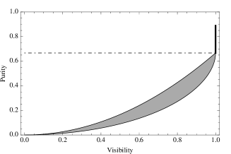
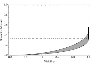
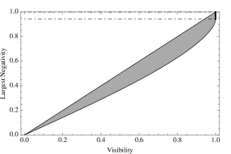
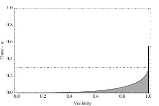
Figure 2: The ranges of entanglement measures studied in this paper as a function of the visibility of the far-field interference pattern. The atoms are pinned at the vertices of an equilateral triangle, and their mutual distance is large. (a) Mixedness of subsystem, (b) geometric measure, (c) bipartite negativity, and (d) three-$\pi$, respectively. In each graph, the range for ${\cal V}<1$ is shown by two curves filled with a gray area, and the thick vertical line indicates the range at ${\cal V}=1$. The asymptotic values for ${\cal V}\to 1$ from below are shown by the dashed-dotted lines.

(d) Three-$\pi$: All entanglement measures studied previously do not vanish when $c_{3}\to 0$. In other words, they are insensitive to genuine tripartite entanglement, but are rather related to entanglement stemming both from bipartite and tripartite entanglements. This is seen from their definitions that all three entanglement measures do not vanish when the problem reduces to the two-atom case (i.e., $c_{1}\geq c_{2}>c_{3}=0$).

To examine the relation to genuine tripartite entanglement measure, the so-called three-$\pi$ is examined, which has a similar origin as the tangle CKW ; OF . This is expressed in terms of the $c_{j}$ as

$${\cal N}_{\pi}=\frac{4}{3}\sum_{j=1}^{3}c_{j}^{4}\left(\sqrt{1+4c_{1}^{2}c_{2}^{2}c_{3}^{2}/c_{j}^{6}}-1\right)\,.$$ (54)

As is easily checked, ${\cal N}_{\pi}=0$ holds when $c_{3}\to 0$ showing that this entanglement measure is only sensitive to genuine tripartite entanglement.

When $c_{1}\leq c_{2}+c_{3}$ the range of the three-$\pi$ is $0<{\cal N}_{\pi}\leq 4(\sqrt{5}-1)/9$, where the upper bound is attained by the W-state and the infimum is obtained for states with $c_{3}\to 0$. When $c_{1}>c_{2}+c_{3}$, the three-$\pi$ is bounded by

$$0<{\cal N}_{\pi}\leq{\cal N}_{\pi}^{\mathrm{max}}\,,$$ (55)

where the infimum is again obtained for states with $c_{3}\to 0$. The upper bound is found for the state with $c_{2}=c_{3}=\sqrt{(1-\upsilon)/2(3+\upsilon)}$ and reads

$${\cal N}_{\pi}^{\mathrm{max}}=\frac{2}{3(3+\upsilon)^{2}}[4(1+\upsilon)\sqrt{5+6\upsilon+5\upsilon^{2}}\\ +(1-\upsilon)\sqrt{(1-\upsilon)(17+5\upsilon)}-(9+14\upsilon+9\upsilon^{2})]\,.$$ (56)

The upper bound converges to the value $2(4\sqrt{5}+\sqrt{17}-9)/27$ $(=0.3012\dots)$ as ${\cal V}\to 1$ from below.

The results are plotted in Fig. 2, (a) mixedness of subsystem, (b) geometric measure, (c) bipartite negativity, and (d) three-$\pi$, respectively. In each graph, the range for ${\cal V}<1$ is shown by two curves filled with a gray area, and the thick vertical line indicates the range at ${\cal V}=1$. The asymptotic values for ${\cal V}\to 1$ from below are shown by the dashed-dotted lines.

IV.3.2 Summary of the results

Let us summarize the obtained relations between the fringe visibility and the four entanglement measures and discuss some consequences of them.

First, the mixedness of the subsystem and the geometric measure exhibit similar behaviors showing jumps in the ranges when ${\cal V}\to 1$ from below. These jumps also exist in the three-$\pi$ case, and result in detecting the amount of entanglement around the full visibility with less accuracy. The appearance of these jumps is partly due to the fact that interference visibility defined by (2) is a quantity closely related to a bipartite system whereas the mixedness of the subsystem and geometric measure are related to both bipartite and tripartite entanglement, and the three-$\pi$ is only related to tripartite entanglement.

Second, Fig. 2 shows that interference visibility can reasonably be used to detect the amount of bipartite entanglement in the W-like state for all values of interference visibility. Remarkably, the upper bound is exactly equal to the largest amount of bipartite negativity with respect to all possible bipartite separations and does not show any jumps when the visibility approaches its maximal value ${\cal V}=1$ from below.

Last, Fig. 2 clearly indicates that the interference visibility is a poor witness of the genuine tripartite entanglement initially present in the atomic system. In particular, getting a far-field interference pattern with full visibility ${\cal V}=1$ does not tell anything at all about the least amount of tripartite entanglement initially present. This result is not really surprising since (39) shows that the interference pattern directly depends on the products $c_{i}c_{j}$. As mentioned, these products identify with the concurrence of the two-atom reduced states obtained by tracing out one atom. It is thus obvious that the interference pattern perfectly encodes some bipartite entanglement properties of the atomic system, but is less sensitive to genuine tripartite entanglement properties.

IV.4 State tomography for the W-like states

In this last section, a state tomography is briefly discussed for the W-like states (28) from information contained in the far-field interference pattern by observing spontaneously emitted photons. The coefficients $c_{j}$ can be extracted simply by taking a few points of the interference pattern (39). Because of the normalization condition of the state, one needs at least three different points to reconstruct the state.

When the W-like initial state has complex coefficients $c_{j}\rightarrow c_{j}\exp\mathrm{i}\phi_{j}$, the full state tomography also needs to find the phases $\phi_{j}$. Since the global phase of the state is irrelevant $c_{1}$ can set to be real. The remaining phases $\phi_{2}$ and $\phi_{3}$ are incorporated in the interference pattern through the replacements $\theta_{j}\to\hat{\theta}_{j}$; $\hat{\theta}_{1}=\theta_{1}+\phi_{2}-\phi_{3}$, $\hat{\theta}_{2}=\theta_{2}-\phi_{3}$, $\hat{\theta}_{3}=\theta_{3}+\phi_{2}$. This shows that these phases $\phi_{j}$ are merely responsible for a shift of the interference pattern. Knowing the position of the fringes, one can extract $\phi_{2}$ and $\phi_{3}$, thus completing the state tomography. We comment that a more complicated analysis is needed when the initial atomic state is mixed. The full tomography may well be possible when the atoms are separated by a distance on the order of optical atomic transition wavelength.

V Conclusion and outlook

In this paper, a system of two-level atoms has been considered when initially prepared in the subspace spanned by the first excited atomic states without photons and releasing a spontaneous photon in the course of time. Some detailed analysis has been given about what kind of information the observation of the far-field interference pattern can help reveal on the amount of entanglement present in the initial atomic state.

In the two-atom case, a previous known result is confirmed showing that the interference visibility indeed converges to the concurrence of the initial atomic state provided the two atomic qubits are far apart. For finite relative distances between the qubits, the deviation of the visibility from the concurrence is calculated numerically. It is found that this deviation is small whenever the qubits are separated by a distance $r$ which is a multiple integer of half the wavelength $\lambda_{0}$ associated to the optical atomic transition. A complete state tomography about the state is shown to be possible provided the two atoms are sufficiently close to each other.

In the three-atom case, the family of W-like states has been considered and the relations between the interference visibility and several known entanglement measures have been analyzed. Bounds have been derived analytically for the amount of entanglement present in the initial state when the interference visibility is given. Our results show that the interference visibility is closely related to the bipartite entanglement properties of the atoms. In particular, it is shown that the interference visibility is directly related to the maximal bipartite negativity.

Two possible extensions of this work are to be mentioned. First, the possibility of detecting genuine multipartite entanglement by defining a suitable interference visibility for multipath interferometers. Second, the analysis of the wave-particle duality aspects in the three-atom case when the atoms have an internal structure allowing for the storage of which-path information. These issues shall be investigated in the future.

Appendix A Entanglement measures

Definitions of the entanglement measures used in this paper are listed. All these measures take on values between 0 and 1 as a convention and are defined for two-qubit and three-qubit systems living in the Hilbert space $({\mathbb{C}}^{2})^{\otimes n}$ ($n=2,3$) of the forms (17) and (28). For more precise definitions of these entanglement measures and for an account of their properties, we refer to Refs. PV ; Horodecki and references therein.

A.1 Concurrence

The concurrence of a general two-qubit state $\rho$ is defined by

$$C(\rho)\equiv\max\{0,\sqrt{\lambda_{1}}-\sqrt{\lambda_{2}}-\sqrt{\lambda_{3}}-\sqrt{\lambda_{4}}\}\,,$$ (57)

where $\lambda_{1}\geq\lambda_{2}\geq\lambda_{3}\geq\lambda_{4}$ are the eigenvalues of $\sqrt{\rho}\,(\sigma_{y}^{(1)}\!\otimes\sigma^{(2)}_{y})\rho^{*}\,(\sigma^{(1)}_{y}\!\otimes\sigma^{(2)}_{y})\sqrt{\rho}$. The $y$ component of the Pauli spin operator is written as $\sigma^{(j)}_{y}=-\mathrm{i}|e\rangle\langle g|+\mathrm{i}|g\rangle\langle e|$, and $\rho^{*}$ denotes the complex conjugate of the state $\rho$.

A.2 Negativity

The negativity of a bipartite system, described by a state $\rho$, is defined as twice the sum of the negative eigenvalues of the state $\rho^{T_{j}}$ obtained by partial transpose with respect to one subsystem. This can be formally expressed as

$${\cal N}(\rho)=||\rho^{T_{1}}||-1=||\rho^{T_{2}}||-1\,,$$ (58)

where the symbol $T_{j}$ denotes the partial transpose with respect to the $j$th subsystem and $||X||$ is the trace class norm of the operator $X$. By convention the negativity of the two-qubit Bell states is set to 1.

For multipartite system, the negativity is defined by the bipartite partitions of the system. For example, ${\cal N}_{j}(\rho)=||\rho^{T_{j}}||-1$ can be defined to quantify the entanglement between the $j$th qubit and the rest of the system.

A.3 Mixedness of subsystem

The mixedness of the subsystem as an entanglement measure in a pure state $\rho=|\psi\rangle\langle\psi|$ is defined by the arithmetical mean of the mixedness associated to each one-qubit reduced states obtained from $\rho$. For the three-atom case for example, it reads

$$M(\rho) =\frac{1}{3}(S(\rho_{1})+S(\rho_{2})+S(\rho_{3}))\,,$$ (59)

$$S(\rho_{j}) =2(1-\mathop{\mathrm{Tr}}\rho_{j}^{2})\,,$$ (60)

where $\rho_{1}=\mathop{\mathrm{Tr}}_{2,3}\rho$, and so on. In several papers, this entanglement measure coincides with the definition of visibility (e.g., Ref. Durr ; JB03 ; Tessier ; JB07 ).

A.4 Geometric measure

The geometric measure for an $n$-qubit system described by a pure state $|\psi\rangle$ is defined by the distance between $|\psi\rangle$ and the closest product state

$$E_{g}(\rho)=\min_{|\phi\rangle\in{\rm Pro}}||\psi\rangle-|\phi\rangle|^{2}\,,$$ (61)

where ${\rm Pro}$ represents the space of product states within the Hilbert space ${\mathbb{C}}^{\otimes n}$.

A.5 Three-$\pi$

Several authors have introduced and studied this measure by following the idea which led to the tangle in Ref. CKW . The most convenient construction appeared in Ref. OF with the definition

$${\cal N}_{\pi}(\rho) =\frac{1}{3}(\pi_{1}+\pi_{2}+\pi_{3})\,,$$ (62)

$$\pi_{j} ={\cal N}^{2}_{j}(\rho)+{\cal N}^{2}(\rho_{j})-\sum_{j=1}^{3}{\cal N}^{2}(\rho_{j})\,,$$ (63)

and ${\cal N}(\rho_{j})$ is the negativity of the reduced state over the $j$th qubit []i.e., $\rho_{j}=\mathop{\mathrm{Tr}}_{j}(\rho)$. This can be written more compactly as

$${\cal N}_{\pi}(\rho)=\frac{1}{3}\sum_{j=1}^{3}[{\cal N}^{2}_{j}(\rho)-2{\cal N}^{2}(\rho_{j})]\,.$$ (64)

References

- (1) See for example, P. Zoller, et al., Eur. Phys. J. D 36, 203 (2005) and references therein.
- (2) Quantum State Estimation, Lecture Notes in Physics, Vol. 649, edited by M. Paris and J. Řeháček, (Springer, Berlin, 2004).
- (3) G. Jaeger, A. Shimony, and L. Vaidman, Phys. Rev. A 51, 54 (1995).
- (4) B.-G. Englert and J. A. Bergou, Opt. Comm. 179, 337 (2000) and references therein.
- (5) M. Jakob and J. A. Bergou, e-print, arXiv: quant-ph/0302075.
- (6) This makes perfect sense as the only way to get a separable state from is indeed to set , in which case reduces to a weighted statistical mixture of the separable states and for which no interference is expected in the far-field. In other words, coherence has been lost. The argument has to be taken with caution as will be seen in Sec. III B. The interference exists in the far-field even for if the atoms are close enough.
- (7) S. Dürr, Phys. Rev. A 64, 042113 (2001).
- (8) T. E. Tessier, Found. Phys. Lett. 18, 107 (2005).
- (9) A. Hosoya, A. Carlini, and S. Okano, Int. J. Mod. Phys. C 17, 493 (2006).
- (10) M. Jakob and J. A. Bergou, Phys. Rev. A 76, 052107 (2007) and references therein.
- (11) B. -G. Englert, D. Kaszlikowski, L. C. Kwek, and W. H. Chee, Int. J. Quant. Inf. 6, 129 (2008).
- (12) J. Eisert and M. B. Plenio, J. Mod. Opt. 46, 145 (1999).
- (13) T.-C. Wei, K. Nemoto, P. M. Goldbart, P. G. Kwiat, W. J. Munro, and F. Verstraete, Phys. Rev. A 67, 022110 (2003) and references therein.
- (14) F. Verstraete, K. Audenaert, J. Dehaene, and B. De Moor, J. Phys. A 34, 10327 (2001).
- (15) C. Cohen-Tannoudji, J. Dupont-Roc, and G. Grynberg, Atom-Photon Interactions: Basic Processes and Applications (Wiley-Interscience, New York, 1992).
- (16) As usual, the bare atomic angular transition frequency gets renormalized by the Lamb shift radiative correction. From now on, denotes this dressed atomic angular transition frequency.
- (17) T. Scholak, F. Mintert, and C. Müller, Europhys. Lett. 83, 60006 (2008).
- (18) W. Dür, G. Vidal, and J. I. Cirac, Phys. Rev. A 62, 062314 (2000).
- (19) L. Tamaryan, D. K. Park, and S. Tamaryan, Phys. Rev. A 77, 022325 (2008).
- (20) V. Coffman, J. Kundu, and W. K. Wootters, Phys. Rev. A 61, 052306 (2000).
- (21) Y. -C. Ou and H. Fan, Phys. Rev. A 75, 062308 (2007).
- (22) M. B. Plenio and S. Virmani, Quant. Inf. Comp. 7, 1 (2007).
- (23) R. Horodecki, P. Horodecki, M. Horodecki, and K. Horodecki, Rev. Mod. Phys. 81, 865 (2009).