Principal Component Analysis with Contaminated Data: The High Dimensional Case

Abstract

We consider the dimensionality-reduction problem (finding a subspace approximation of observed data) for contaminated data in the high dimensional regime, where the number of observations is of the same magnitude as the number of variables of each observation, and the data set contains some (arbitrarily) corrupted observations. We propose a High-dimensional Robust Principal Component Analysis (HR-PCA) algorithm that is tractable, robust to contaminated points, and easily kernelizable. The resulting subspace has a bounded deviation from the desired one, achieves maximal robustness – a breakdown point of $50\%$ while all existing algorithms have a breakdown point of zero, and unlike ordinary PCA algorithms, achieves optimality in the limit case where the proportion of corrupted points goes to zero.

I Introduction

The analysis of very high dimensional data – data sets where the dimensionality of each observation is comparable to or even larger than the number of observations – has drawn increasing attention in the last few decades [1, 2]. For example, observations on individual instances can be curves, spectra, images or even movies, where a single observation has dimensionality ranging from thousands to billions. Practical high dimensional data examples include DNA Microarray data, financial data, climate data, web search engine, and consumer data. In addition, the nowadays standard “Kernel Trick” [3], a pre-processing routine which non-linearly maps the observations into a (possibly infinite dimensional) Hilbert space, transforms virtually every data set to a high dimensional one. Efforts of extending traditional statistical tools (designed for the low dimensional case) into this high-dimensional regime are generally unsuccessful. This fact has stimulated research on formulating fresh data-analysis techniques able to cope with such a “dimensionality explosion.”

Principal Component Analysis (PCA) is perhaps one of the most widely used statistical techniques for dimensionality reduction. Work on PCA dates back as early as [4], and has become one of the most important techniques for data compression and feature extraction. It is widely used in statistical data analysis, communication theory, pattern recognition, and image processing [5]. The standard PCA algorithm constructs the optimal (in a least-square sense) subspace approximation to observations by computing the eigenvectors or Principal Components (PCs) of the sample covariance or correlation matrix. Its broad application can be attributed to primarily two features: its success in the classical regime for recovering a low-dimensional subspace even in the presence of noise, and also the existence of efficient algorithms for computation. Indeed, PCA is nominally a non-convex problem, which we can, nevertheless, solve, thanks to the magic of the SVD which allows us to maximize a convex function. It is well-known, however, that precisely because of the quadratic error criterion, standard PCA is exceptionally fragile, and the quality of its output can suffer dramatically in the face of only a few (even a vanishingly small fraction) grossly corrupted points. Such non-probabilistic errors may be present due to data corruption stemming from sensor failures, malicious tampering, or other reasons. Attempts to use other error functions growing more slowly than the quadratic that might be more robust to outliers, result in non-convex (and intractable) optimization problems.

In this paper, we consider a high-dimensional counterpart of Principal Component Analysis (PCA) that is robust to the existence of arbitrarily corrupted or contaminated data. We start with the standard statistical setup: a low dimensional signal is (linearly) mapped to a very high dimensional space, after which point high-dimensional Gaussian noise is added, to produce points that no longer lie on a low dimensional subspace. At this point, we deviate from the standard setting in two important ways: (1) a constant fraction of the points are arbitrarily corrupted in a perhaps non-probabilistic manner. We emphasize that these “outliers” can be entirely arbitrary, rather than from the tails of any particular distribution, e.g., the noise distribution; we call the remaining points “authentic”; (2) the number of data points is of the same order as (or perhaps considerably smaller than) the dimensionality. As we discuss below, these two points confound (to the best of our knowledge) all tractable existing Robust PCA algorithms.

A fundamental feature of the high dimensionality is that the noise is large in some direction, with very high probability, and therefore definitions of “outliers” from classical statistics are of limited use in this setting. Another important property of this setup is that the signal-to-noise ratio (SNR) can go to zero, as the $\ell_{2}$ norm of the high-dimensional Gaussian noise scales as the square root of the dimensionality. In the standard (i.e., low-dimensional case), a low SNR generally implies that the signal cannot be recovered, even without any corrupted points.

The Main Result

In this paper, we give a surprisingly optimistic message: contrary to what one might expect given the brittle nature of classical PCA, and in stark contrast to previous algorithms, it is possible to recover such low SNR signals, in the high-dimensional regime, even in the face of a constant fraction of arbitrarily corrupted data. Moreover, we show that this can be accomplished with an efficient (polynomial time) algorithm, which we call High-Dimensional Robust PCA (HR-PCA). The algorithm we propose here is tractable, provably robust to corrupted points, and asymptotically optimal, recovering the exact low-dimensional subspace when the number of corrupted points scales more slowly than the number of “authentic” samples (i.e., when the fraction of corrupted points tends to zero). To the best of our knowledge, this is the only algorithm of this kind. Moreover, it is easily kernelizable.

The proposed algorithm performs a PCA and a random removal alternately. Therefore, in each iteration a candidate subspace is found. The random removal process guarantees that with high probability, one of candidate solutions found by the algorithm is “close” to the optimal one. Thus, comparing all solutions using a (computational efficient) one-dimensional robust variance estimator leads to a “sufficiently good” output. We will make this argument rigorous in the following sections.

Organization and Notation

The paper is organized as follows: In Section II we discuss past work and the reasons that classical robust PCA algorithms fail to extend to the high dimensional regime. In Section III we present the setup of the problem, and the HR-PCA algorithm. We also provide finite sample and asymptotic performance guarantees. Section IV is devoted to the kernelization of HR-PCA. The performance guarantee are proved in Section V. We provide some numerical experiment results in Section VI. Some technical details in the derivation of the performance guarantees are postponed to the appendix.

Capital letters and boldface letters are used to denote matrices and vectors, respectively. A $k\times k$ unit matrix is denoted by $I_{k}$. For $c\in\mathbb{R}$, $[c]^{+}\triangleq\max(0,c)$.We let $\mathcal{B}_{d}\triangleq\{\mathbf{w}\in\mathbb{R}^{d}|\|\mathbf{w}\|\leq 1\}$, and $\mathcal{S}_{d}$ be its boundary. We use a subscript $(\cdot)$ to represent order statistics of a random variable. For example, let $v_{1},\cdots,v_{n}\in\mathbb{R}$. Then $v_{(1)},\cdots,v_{(n)}$ is a permutation of $v_{1},\cdots,v_{n}$, in a non-decreasing order.

II Relation to Past Work

In this section, we discuss past work and the reasons that classical robust PCA algorithms fail to extend to the high dimensional regime.

Much previous robust PCA work focuses on the traditional robustness measurement known as the “breakdown point” [6], i.e., the percentage of corrupted points that can make the output of the algorithm arbitrarily bad. To the best of our knowledge, no other algorithm can handle any constant fraction of outliers with a lower bound on the error in the high-dimensional regime. That is, the best-known breakdown point for this problem is zero. We show that the algorithm we provide has breakdown point of $50\%$, which is the best possible for any algorithm. In addition to this, we focus on providing explicit lower bounds on the performance, for all corruption levels up to the breakdown point.

In the low-dimensional regime where the observations significantly outnumber the variables of each observation, several robust PCA algorithms have been proposed (e.g., [7, 8, 9, 10, 11, 12, 13, 14]). These algorithms can be roughly divided into two classes: (i) performing a standard PCA on a robust estimation of the covariance or correlation matrix; (ii) maximizing (over all unit-norm $\mathbf{w}$) some $r(\mathbf{w})$ that is a robust estimate of the variance of univariate data obtained by projecting the observations onto direction $\mathbf{w}$. Both approaches encounter serious difficulties when applied to high-dimensional data-sets:

• There are not enough observations to robustly estimate the covariance or correlations matrix. For example, the widely-used MVE estimator [15], which treats the Minimum Volume Ellipsoid that covers half of the observations as the covariance estimation, is ill-posed in the high-dimensional case. Indeed, to the best of our knowledge, the assumption that observations far outnumber dimensionality seems crucial for those robust variance estimators to achieve statistical consistency.

• Algorithms that subsample the points, and in the spirit of leave-one-out approaches, attempt in this way to compute the correct principal components, also run into trouble. The constant fraction of corrupted points means the sampling rate must be very low (in particular, leave-one-out accomplishes nothing). But then, due to the high dimensionality of the problem, principal components from one sub-sample to the next, can vary greatly.

• Unlike standard PCA that has a polynomial computation time, the maximization of $r(\mathbf{w})$ is generally a non-convex problem, and becomes extremely hard to solve or approximate as the dimensionality of $\mathbf{w}$ increases. In fact, the number of the local maxima grows so fast that it is effectively impossible to find a sufficiently good solution using gradient-based algorithms with random re-initialization.

We now discuss in greater detail three pitfalls some existing algorithms face in high dimensions.

Diminishing Breakdown Point: The breakdown point measures the fraction of outliers required to change the output of a statistics algorithm arbitrarily. If an algorithm’s breakdown point has an inverse dependence on the dimensionality, then it is unsuitable in our regime. Many algorithms fall into this category. In [16], several covariance estimators including M-estimator [17], Convex Peeling [18, 19], Ellipsoidal Peeling [20, 21], Classical Outlier Rejection [22, 23], Iterative Deletion [24] and Iterative Trimming [25, 26] are all shown to have breakdown points upper-bounded by the inverse of the dimensionality, hence not useful in the regime of interest.

Noise Explosion: As we define in greater detail below, the model we consider is the standard PCA setup: we observe samples $\mathbf{y}=A\mathbf{x}+\mathbf{n}$, where $A$ is an $n\times d$ matrix, $\mathbf{n}\sim\mathcal{N}(0,I_{m})$, and $n\approx m>>d$. Thus, $n$ is the number of samples, $m$ the dimension, and $d$ the dimension of $\mathbf{x}$ and thus the number of principal components. Let $\sigma_{1}$ denote the largest singular value of $A$. Then, $\mathbb{E}(\|\mathbf{n}\|_{2})=\sqrt{m}$, (in fact, the magnitude sharply concentrates around $\sqrt{m}$), while $\mathbb{E}(\|A\mathbf{x}\|_{2})=\sqrt{\mathrm{trace}(A^{\top}A)}\leq\sqrt{d}\sigma_{1}$. Unless $\sigma_{1}$ grows very quickly (namely, at least as fast as $\sqrt{m}$) the magnitude of the noise quickly becomes the dominating component of each authentic point we obtain. Because of this, several perhaps counter-intuitive properties hold in this regime. First, any given authentic point is with overwhelming probability very close to orthogonal to the signal space (i.e., to the true principal components). Second, it is possible for a constant fraction of corrupted points all with a small Mahalanobis distance to significantly change the output of PCA. Indeed, by aligning $\lambda n$ points of magnitude some constant multiple of $\sigma_{1}$, it is easy to see that the output of PCA can be strongly manipulated – on the other hand, since the noise magnitude is $\sqrt{m}\approx\sqrt{n}$ in a direction perpendicular to the principal components, the Mahalanobis distance of each corrupted point will be very small. Third, and similarly, it is possible for a constant fraction of corrupted points all with small Stahel-Donoho outlyingness to significantly change the output of PCA. Stahel-Donoho outlyingness is defined as:

$$u_{i}\triangleq\sup_{\|\mathbf{w}\|=1}\frac{|\mathbf{w}^{\top}\mathbf{y}_{i}-\mathrm{med}_{j}(\mathbf{w}^{\top}\mathbf{y}_{j})|}{\mathrm{med}_{k}|\mathbf{w}^{\top}\mathbf{y}_{k}-\mathrm{med}_{j}(\mathbf{w}^{\top}\mathbf{y}_{j})|}.$$

To see that this can be small, consider the same setup as for the Mahalanobis example: small magnitude outliers, all aligned along one direction. Then the Stahel-Donoho outlyingness of such a corrupted point is $O(\sigma_{1}/\lambda)$. For a given authentic sample $\mathbf{y}_{i}$, take $\mathbf{v}=\mathbf{y}_{i}/\|\mathbf{y}_{i}\|$. On the projection of $\mathbf{v}$, all samples except $\mathbf{y}_{i}$ follow a Gaussian distribution with a variance roughly $1$, because $\mathbf{v}$ only depends on $\mathbf{y}_{i}$ (recall that $\mathbf{v}$ is nearly orthogonal to $A$). Hence the S-D outlyingness of a sample is of $\Theta(\sqrt{m})$, which is much larger than that of a corrupted point.

The Mahalanobis distance and the S-D outlyingness are extensively used in existing robust PCA algorithms. For example, Classical Outlier Rejection, Iterative Deletion and various alternatives of Iterative Trimmings all use the Mahalanobis distance to identify possible outliers. Depth Trimming [16] weights the contribution of observations based on their S-D outlyingness. More recently, the ROBPCA algorithm proposed in [27] selects a subset of observations with least S-D outlyingness to compute the $d$-dimensional signal space. Thus, in the high-dimensional case, these algorithms may run into problems since neither Mahalanobis distance nor S-D outlyingness are valid indicator of outliers. Indeed, as shown in the simulations, the empirical performance of such algorithms can be worse than standard PCA, because they remove the authentic samples.

Algorithmic Tractability: There are algorithms that do not rely on Mahalanobis distance or S-D outlyingness, and have a non-diminishing breakdown point, namely Minimum Volume Ellipsoid (MVE), Minimum Covariance Determinant (MCD) [28] and Projection-Pursuit [29]. MVE finds the minimum volume ellipsoid that covers a certain fraction of observations. MCD finds a fraction of observations whose covariance matrix has a minimal determinant. Projection Pursuit maximizes a certain robust univariate variance estimator over all directions.

MCD and MVE are combinatorial, and hence (as far as we know) computationally intractable as the size of the problem scales. More difficult yet, MCD and MVE are ill-posed in the high-dimensional setting where the number of points (roughly) equals the dimension, since there exist infinitely many zero-volume (determinant) ellipsoids satisfying the covering requirement. Nevertheless, we note that such algorithms work well in the low-dimensional case, and hence can potentially be used as a post-processing procedure of our algorithm by projecting all observations to the output subspace to fine tune the eigenvalues and eigenvectors we produce.

Maximizing a robust univariate variance estimator as in Projection Pursuit, is also non-convex, and thus to the best of our knowledge, computationally intractable. In [30], the authors propose a fast Projection-Pursuit algorithm, avoiding the non-convex optimization problem of finding the optimal direction, by only examining the directions of each sample. While this is suitable in the classical regime, in the high-dimensional setting this algorithm fails, since as discussed above, the direction of each sample is almost orthogonal to the direction of true principal components. Such an approach would therefore only be examining candidate directions nearly orthogonal to the true maximizing directions.

Low Rank Techniques: Finally, we discuss the recent paper [31]. In this work, the authors adapt techniques from low-rank matrix approximation, and in particular, results similar to the matrix decomposition results of [32], in order to recover a low-rank matrix $L_{0}$ from highly corrupted measurements $M=L_{0}+S_{0}$, where the noise term, $S_{0}$, is assumed to have a sparse structure. This models the scenario where we have perfect measurement of most of the entries of $L_{0}$, and a small (but constant) fraction of the random entries are arbitrarily corrupted. This work is much closer in spirit, in motivation, and in terms of techniques, to the low-rank matrix completion and matrix recovery problems in [33, 34, 35] than the setting we consider and the work presented herein. In particular, in our setting, each corrupted point can change every element of a column of $M$, and hence render the low rank approach invalid.

III HR-PCA: The Algorithm

The algorithm of HR-PCA is presented in this section. We start with the mathematical setup of the problem in Section III-A. The HR-PCA algorithm as well as its performance guarantee are then given in Section III-B.

III-A Problem Setup

We now define in detail the problem described above.

• The “authentic samples” $\mathbf{z}_{1},\dots,\mathbf{z}_{t}\in\mathbb{R}^{m}$ are generated by $\mathbf{z}_{i}=A\mathbf{x}_{i}+\mathbf{n}_{i}$, where $\mathbf{x}_{i}\in\mathbb{R}^{d}$ (the “signal”) are i.i.d. samples of a random variable $\mathbf{x}$, and $\mathbf{n}_{i}$ (the “noise”) are independent realizations of $\mathbf{n}\sim\mathcal{N}(\mathbf{0},I_{m})$. The matrix $A\in\mathbb{R}^{m\times d}$ and the distribution of $\mathbf{x}$ (denoted by $\mu$) are unknown. We do assume, however, that the distribution $\mu$ is absolutely continuous with respect to the Borel measure, it is spherically symmetric (and in particular, $\mathbf{x}$ has mean zero and variance $I_{d}$) and it has light tails, specifically, there exist constants $K,C>0$ such that $\mathrm{Pr}(\|\mathbf{x}\|\geq x)\leq K\exp(-Cx)$ for all $x\geq 0$. Since the distribution $\mu$ and the dimension d are both fixed, as m,n scale, the assumption that mu is spherically symmetric can be easily relaxed, and the expense of potentially significant notational complexity.

• The outliers (the corrupted data) are denoted $\mathbf{o}_{1},\dots,\mathbf{o}_{n-t}\in\mathbb{R}^{m}$ and as emphasized above, they are arbitrary (perhaps even maliciously chosen). We denote the fraction of corrupted points by $\lambda\stackrel{{\scriptstyle\bigtriangleup}}{{=}}(n-t)/{n}$.

• We only observe the contaminated data set

  $$\mathcal{Y}\triangleq\{\mathbf{y}_{1}\dots,\mathbf{y}_{n}\}=\{\mathbf{z}_{1},\dots,\mathbf{z}_{t}\}\bigcup\{\mathbf{o}_{1},\dots,\mathbf{o}_{n-t}\}.$$

  An element of $\mathcal{Y}$ is called a “point”.

Given these contaminated observations, we want to recover the principal components of $A$, equivalently, the top eigenvectors, $\overline{\mathbf{w}}_{1},\dots,\overline{\mathbf{w}}_{d}$ of $AA^{\top}$. That is, we seek a collection of orthogonal vectors $\mathbf{w}_{1},\dots,\mathbf{w}_{d}$, that maximize the performance metric called the Expressed Variance:

$${\rm E.V.}\triangleq\frac{\sum_{j=1}^{d}\mathbf{w}_{j}^{\top}AA^{\top}\mathbf{w}_{j}}{\sum_{j=1}^{d}\overline{\mathbf{w}}_{j}^{\top}AA^{\top}\overline{\mathbf{w}}_{j}}=\frac{\sum_{j=1}^{d}\mathbf{w}_{j}^{\top}AA^{\top}\mathbf{w}_{j}}{\mathrm{trace}(AA^{\top})}.$$

The E.V. is always less than one, with equality achieved exactly when the vectors $\mathbf{w}_{1},\dots,\mathbf{w}_{d}$ have the span of the true principal components $\{\overline{\mathbf{w}}_{1},\dots,\overline{\mathbf{w}}_{d}\}$. When $d=1$, the Expressed Variance relates to another natural performance metric — the angle between $\mathbf{w}_{1}$ and $\overline{\mathbf{w}}_{1}$ — since by definition $E.V.(\mathbf{w}_{1})=\cos^{2}(\angle(\mathbf{w}_{1},\,\overline{\mathbf{w}}_{1}))$. The Expressed Variance represents the portion of signal $A\mathbf{x}$ being expressed by $\mathbf{w}_{1},\dots,\mathbf{w}_{d}$. Equivalently, $1-E.V.$ is the reconstruction error of the signal.

It is natural to expect that the ability to recover vectors with a high expressed variance depends on $\lambda$, the fraction of corrupted points — in addition, it depends on the distribution, $\mu$ generating the (low-dimensional) points $\mathbf{x}$, through its tails. If $\mu$ has longer tails, outliers that affect the variance (and hence are far from the origin) and authentic samples in the tail of the distribution, become more difficult to distinguish. To quantify this effect, we define the following “tail weight” function $\mathcal{V}:[0,\,1]\rightarrow[0,\,1]$:

$$\mathcal{V}(\alpha)\triangleq\int_{-c_{\alpha}}^{c_{\alpha}}x^{2}\overline{\mu}(dx);$$

where $\overline{\mu}$ is the one-dimensional margin of $\mu$ (recall that $\mu$ is spherically symmetric), and $c_{\alpha}$ is such that $\overline{\mu}([-c_{\alpha},c_{\alpha}]=\alpha)$. Since $\mu$ has a density function, $c_{\alpha}$ is well defined. Thus, $\mathcal{V}(\cdot)$ represents how the tail of $\overline{\mu}$ contributes to its variance. Notice that $\mathcal{V}(0)=0$, $\mathcal{V}(1)=1$, and $\mathcal{V}(\cdot)$ is continuous since $\mu$ has a density function. For notational convenience, we simply let $\mathcal{V}(x)=0$ for $x<0$, and $\mathcal{V}(x)=\infty$ for $x>1$.

The bounds on the quality of recovery, given in Theorems 1 and 2 below, are functions of $\eta$ and the function $\mathcal{V}(\cdot)$.

High Dimensional Setting and Asymptotic Scaling

In this paper, we focus on the case where $n\sim m\gg d$ and $\mathrm{trace}(A^{\top}A)\gg 1$. That is, the number of observations and the dimensionality are of the same magnitude, and much larger than the dimensionality of $\mathbf{x}$; the trace of $A^{\top}A$ is significantly larger than $1$, but may be much smaller than $n$ and $m$. In our asymptotic scaling, $n$ and $m$ scale together to infinity, while $d$ remains fixed. The value of $\sigma_{1}$ also scales to infinity, but there is no lower bound on the rate at which this happens (and in particular, the scaling of $\sigma_{1}$ can be much slower than the scaling of $m$ and $n$).

While we give finite-sample results, we are particularly interested in the asymptotic performance of HR-PCA when the dimension and the number of observations grow together to infinity. Our asymptotic setting is as follows. Suppose there exists a sequence of sample sets $\{\mathcal{Y}(j)\}=\{\mathcal{Y}(1),\mathcal{Y}(2),\dots\}$, where for $\mathcal{Y}(j)$, $n(j)$, $m(j)$, $A(j)$, $d(j)$, etc., denote the corresponding values of the quantities defined above. Then the following must hold for some positive constants $c_{1},c_{2}$:

$$\begin{split}&\lim_{j\rightarrow\infty}\frac{n(j)}{m(j)}=c_{1};\quad d(j)\leq c_{2};\quad m(j)\uparrow+\infty;\\ &\mathrm{trace}(A(j)^{\top}A(j))\uparrow+\infty.\end{split}$$ (1)

While $\mathrm{trace}(A(j)^{\top}A(j))\uparrow+\infty$, if it scales more slowly than $\sqrt{m(j)}$, the SNR will asymptotically decrease to zero.

III-B Key Idea and Main Algorithm

For $\mathbf{w}\in\mathcal{S}_{m}$, we define the Robust Variance Estimator (RVE) as $\overline{V}_{\hat{t}}(\mathbf{w})\triangleq\frac{1}{n}\sum_{i=1}^{\hat{t}}|\mathbf{w}^{\top}\mathbf{y}|^{2}_{(i)}$. This stands for the following statistics: project $\mathbf{y}_{i}$ onto the direction $\mathbf{w}$, replace the furthest (from original) $n-\hat{t}$ samples by $0$, and then compute the variance. Notice that the RVE is always performed on the original observed set $\mathcal{Y}$.

The main algorithm of HR-PCA is as given below.

Algorithm 1

HR-PCA Input: Contaminated sample-set $\mathcal{Y}=\{\mathbf{y}_{1},\dots,\mathbf{y}_{n}\}\subset\mathbb{R}^{m}$, $d$, $\overline{T}$, $\hat{t}$. Output: $\mathbf{w}^{*}_{1},\dots,\mathbf{w}^{*}_{d}$. Algorithm: 1. Let $\hat{\mathbf{y}}_{i}:=\mathbf{y}_{i}$ for $i=1,\dots n$; $s:=0$; $\mathrm{Opt}:=0$. 2. While $s\leq\overline{T}$, do (a) Compute the empirical variance matrix $$\hat{\Sigma}:=\frac{1}{n-s}\sum_{i=1}^{n-s}\hat{\mathbf{y}}_{i}\hat{\mathbf{y}}_{i}^{\top}.$$ (b) Perform PCA on $\hat{\Sigma}$. Let $\mathbf{w}_{1},\dots,\mathbf{w}_{d}$ be the $d$ principal components of $\hat{\Sigma}$. (c) If $\sum_{j=1}^{d}\overline{V}_{\hat{t}}(\mathbf{w}_{j})>\mathrm{Opt}$, then let $\mathrm{Opt}:=\sum_{j=1}^{d}\overline{V}_{\hat{t}}(\mathbf{w}_{j})$ and let $\mathbf{w}^{*}_{j}:=\mathbf{w}_{j}$ for $j=1,\cdots,d$. (d) Randomly remove a point from $\{\hat{\mathbf{y}}_{i}\}_{i=1}^{n-s}$ according to $$\mathrm{Pr}(\hat{\mathbf{y}}_{i}\mbox{ is removed})\propto\sum_{j=1}^{d}(\mathbf{w}_{j}^{\top}\hat{\mathbf{y}}_{i})^{2};$$ (e) Denote the remaining points by $\{\hat{\mathbf{y}}_{i}\}_{i=1}^{n-s-1}$; (f) $s:=s+1$. 3. Output $\mathbf{w}^{*}_{1},\dots,\mathbf{w}^{*}_{d}$. End.

Intuition on Why The Algorithm Works

On any given iteration, we select candidate directions based on standard PCA – thus directions chosen are those with largest empirical variance. Now, given a candidate direction, $\mathbf{w}$, our robust variance estimator measures the variance of the $(n-\hat{t})$-smallest points projected in that direction. If this is large, it means that many of the points have a large variance in this direction – the points contributing to the robust variance estimator, and the points that led to this direction being selected by PCA. If the robust variance estimator is small, it is likely that a number of the largest variance points are corrupted, and thus removing one of them randomly, in proportion to their distance in the direction $\mathbf{w}$, will remove a corrupted point.

Thus in summary, the algorithm works for the following intuitive reason. If the corrupted points have a very high variance along a direction with large angle from the span of the principal components, then with some probability, our algorithm removes them. If they have a high variance in a direction “close to” the span of the principal components, then this can only help in finding the principal components. Finally, if the corrupted points do not have a large variance, then the distortion they can cause in the output of PCA is necessarily limited.

The remainder of the paper makes this intuition precise, providing lower bounds on the probability of removing corrupted points, and subsequently upper bounds on the maximum distortion the corrupted points can cause, i.e., lower bounds on the Expressed Variance of the principal components our algorithm recovers.

There are two parameters to tune for HR-PCA, namely $\hat{t}$ and $\overline{T}$. Basically, $\hat{t}$ affects the performance of HR-PCA through Inequality 2, and as a rule of thumb we can set $\hat{t}=t$ when no a priori information of $\mu$ exists. $\overline{T}$ does not affect the performance as long as it is large enough, hence we can simply set $T=n-1$, although when $\lambda$ is small, a smaller $T$ leads to the same solution with less computational cost.

The correctness of HR-PCA is shown in the following theorems for both the finite-sample bound, and the asymptotic performance.

Theorem 1 (Finite Sample Performance)

Let the algorithm above output $\{\mathbf{w}_{1},\dots,\mathbf{w}_{d}\}$. Fix a $\kappa>0$, and let $\tau=\max(m/n,1)$. There exists a universal constant $c_{0}$ and a constant $C$ which can possible depend on $\hat{t}/t$, $\lambda$, $d$, $\mu$ and $\kappa$, such that for any $\gamma<1$, if $n/\log^{4}n\geq\log^{6}(1/\gamma)$, then with probability $1-\gamma$ the following holds

$$\mathrm{E.V.\{\mathbf{w}_{1},\dots,\mathbf{w}_{d}\}} \geq \left[\frac{\mathcal{V}\left(1-\frac{\lambda(1+\kappa)}{(1-\lambda)\kappa}\right)}{(1+\kappa)}\right]\times\left[\frac{\mathcal{V}\left(\frac{\hat{t}}{t}-\frac{\lambda}{1-\lambda}\right)}{\mathcal{V}\left(\frac{\hat{t}}{t}\right)}\right]$$

$$-\left[\frac{8\sqrt{c_{0}\tau d}}{\mathcal{V}\left(\frac{\hat{t}}{t}\right)}\right](\mathrm{trace}(AA^{\top}))^{-1/2}-\left[\frac{2c_{0}\tau}{\mathcal{V}\left(\frac{\hat{t}}{t}\right)}\right](\mathrm{trace}(AA^{\top}))^{-1}-C\frac{\log^{2}n\log^{3}(1/\gamma)}{\sqrt{n}}.$$

The last three terms go to zero as the dimension and number of points scale to infinity, i.e., as $n.m\rightarrow\infty$. Therefore, we immediately obtain:

Theorem 2 (Asymptotic Performance)

Given a sequence of $\{\mathcal{Y}(j)\}$, if the asymptotic scaling in Expression (1) holds, and $\limsup\lambda(j)\leq\lambda^{*}$, then the following holds in probability when $j\uparrow\infty$ (i.e., when $n,m\uparrow\infty$),

$$\lim\inf_{j}\mathrm{E.V.\{\mathbf{w}_{1}(j),\dots,\mathbf{w}_{d}(j)\}}\geq\max_{\kappa}\left[\frac{\mathcal{V}\left(1-\frac{\lambda^{*}(1+\kappa)}{(1-\lambda^{*})\kappa}\right)}{(1+\kappa)}\right]\times\left[\frac{\mathcal{V}\left(\frac{\hat{t}}{t}-\frac{\lambda^{*}}{1-\lambda^{*}}\right)}{\mathcal{V}\left(\frac{\hat{t}}{t}\right)}\right].$$ (2)

Remark 1

The bounds in the two bracketed terms in the asymptotic bound may be, roughly, explained as follows. The first term is due to the fact that the removal procedure may well not remove all large-magnitude corrupted points, while at the same time, some authentic points may be removed. The second term accounts for the fact that not all the outliers may have large magnitude. These will likely not be removed, and will have some (small) effect on the principal component directions reported in the output.

Remark 2

The terms in the second line of Theorem 1 go to zero as $n,m\rightarrow\infty$, and therefore the proving Theorem 1 immediately implies Theorem 2.

Remark 3

If $\lambda(j)\downarrow 0$, i.e., the number of corrupted points scales sublinearly (in particular, this holds when there are a fixed number of corrupted points), then the right-hand-side of Inequality (2) equals $1$, i.e., HR-PCA is asymptotically optimal. This is in contrast to PCA, where the existence of even a single corrupted point is sufficient to bound the output arbitrarily away from the optimum.

Remark 4

The breakdown point of HR-PCA converges to $50\%$. Note that since $\mu$ has a density function, $\mathcal{V}(\alpha)>0$ for any $\alpha\in(0,1]$. Therefore, for any $\lambda<1/2$, if we set $\hat{t}$ to any value in $(\lambda n,t]$, then there exists $\kappa$ large enough such that the right-hand-side is strictly positive (recall that $t=(1-\lambda)n$). The breakdown point hence converges to $50\%$. Thus, HR-PCA achieves the maximal possible break-down point (note that a breakdown point greater than $50\%$ is never possible, since then there are more outliers than samples.

The graphs in Figure 1 illustrate the lower-bounds of asymptotic performance if the 1-dimension marginal of $\mu$ is the Gaussian distribution or the Uniform distribution.

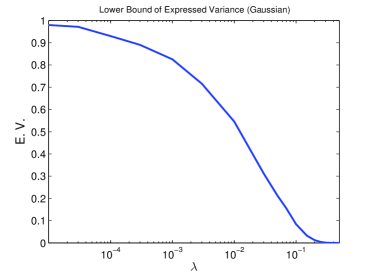
(a) Gaussian distribution	(b) Uniform distribution

Figure 1: Lower Bounds of Asymptotic Performance.

IV Kernelization

We consider kernelizing HR-PCA in this section: given a feature mapping $\Upsilon(\cdot):\mathbb{R}^{m}\rightarrow\mathcal{H}$ equipped with a kernel function $k(\cdot,\cdot)$, i.e., $\langle\Upsilon(\mathbf{a}),\,\Upsilon(\mathbf{b})\rangle=k(\mathbf{a},\mathbf{b})$ holds for all $\mathbf{a},\mathbf{b}\in\mathbb{R}^{m}$, we perform the dimensionality reduction in the feature space $\mathcal{H}$ without knowing the explicit form of $\Upsilon(\cdot)$.

We assume that $\{\Upsilon(\mathbf{y}_{1}),\cdots,\Upsilon(\mathbf{y}_{n})\}$ is centered at origin without loss of generality, since we can center any $\Upsilon(\cdot)$ with the following feature mapping

$$\hat{\Upsilon}(\mathbf{x})\triangleq\Upsilon(\mathbf{x})-\frac{1}{n}\sum_{i=1}^{n}\Upsilon(\mathbf{y}_{i}),$$

whose kernel function is

$$\hat{k}(\mathbf{a},\mathbf{b})=k(\mathbf{a},\mathbf{b})-\frac{1}{n}\sum_{j=1}^{n}k(\mathbf{a},\mathbf{y}_{j})-\frac{1}{n}\sum_{i=1}^{n}k(\mathbf{y}_{i},\mathbf{b})+\frac{1}{n^{2}}\sum_{i=1}^{n}\sum_{j=1}^{n}k(\mathbf{y}_{i},\mathbf{y}_{j}).$$

Notice that HR-PCA involves finding a set of PCs $\mathbf{w}_{1},\dots,\mathbf{w}_{d}\in\mathcal{H}$, and evaluating $\langle\mathbf{w}_{q},\,\Upsilon(\cdot)\rangle$ (Note that RVE is a function of $\langle\mathbf{w}_{q},\,\Upsilon(\mathbf{y}_{i})\rangle$, and random removal depends on $\langle\mathbf{w}_{q},\,\Upsilon(\hat{\mathbf{y}}_{i})\rangle$). The former can be kernelized by applying Kernel PCA introduced by [36], where each of the output PCs admits a representation

$$\mathbf{w}_{q}=\sum_{j=1}^{n-s}\alpha_{j}(q)\Upsilon(\hat{\mathbf{y}}_{j}).$$

Thus, $\langle\mathbf{w}_{q},\,\Upsilon(\cdot)\rangle$ is easily evaluated by

$$\langle\mathbf{w}_{q},\,\Upsilon(\mathbf{v})\rangle=\sum_{j=1}^{n-s}\alpha_{j}(q)k(\hat{\mathbf{y}}_{j},\mathbf{v});\quad\forall\mathbf{v}\in\mathbb{R}^{m}$$

Therefore, HR-PCA is kernelizable since both steps are easily kernelized and we have the following Kernel HR-PCA.

Algorithm 2

Kernel HR-PCA Input: Contaminated sample-set $\mathcal{Y}=\{\mathbf{y}_{1},\dots,\mathbf{y}_{n}\}\subset\mathbb{R}^{m}$, $d$, $T$, $\hat{n}$. Output: $\boldsymbol{\alpha}^{*}(1),\dots,\boldsymbol{\alpha}^{*}(d)$. Algorithm: 1. Let $\hat{\mathbf{y}}_{i}:=\mathbf{y}_{i}$ for $i=1,\dots n$; $s:=0$; $\mathrm{Opt}:=0$. 2. While $s\leq T$, do (a) Compute the Gram matrix of $\{\hat{\mathbf{y}}_{i}\}$: $$K_{ij}:=k(\hat{\mathbf{y}}_{i},\hat{\mathbf{y}}_{j});\quad i,j=1,\cdots,n-s.$$ (b) Let $\hat{\sigma}^{2}_{1},\cdots,\hat{\sigma}^{2}_{d}$ and $\hat{\boldsymbol{\alpha}}(1),\cdots,\hat{\boldsymbol{\alpha}}(d)$ be the $d$ largest eigenvalues and the corresponding eigenvectors of $K$. (c) Normalize: $\boldsymbol{\alpha}(q):=\hat{\boldsymbol{\alpha}}(q)/\hat{\sigma}_{q}$, so that $\|\mathbf{w}_{q}\|=1$. (d) If $\sum_{q=1}^{d}\overline{V}_{\hat{t}}(\boldsymbol{\alpha}(q))>\mathrm{Opt}$, then let $\mathrm{Opt}:=\sum_{q=1}^{d}\overline{V}_{\hat{t}}(\boldsymbol{\alpha}(q))$ and let $\boldsymbol{\alpha}^{*}(q):=\boldsymbol{\alpha}(q)$ for $q=1,\cdots,d$. (e) Randomly remove a point from $\{\hat{\mathbf{y}}_{i}\}_{i=1}^{n-s}$ according to $$\mathrm{Pr}(\hat{\mathbf{y}}_{i}\mbox{ is removed})\propto\sum_{q=1}^{d}(\sum_{j=1}^{n-s}\alpha_{j}(q)k(\hat{\mathbf{y}}_{j},\hat{\mathbf{y}}_{i}))^{2};$$ (f) Denote the remaining points by $\{\hat{\mathbf{y}}_{i}\}_{i=1}^{n-s-1}$; (g) $s:=s+1$. 3. Output $\boldsymbol{\alpha}^{*}(1),\dots,\boldsymbol{\alpha}^{*}(d)$. End.

Here, the kernelized RVE is defined as

$$\overline{V}_{\hat{t}}(\boldsymbol{\alpha})\triangleq\frac{1}{n}\sum_{i=1}^{\hat{t}}\left[\big{|}\langle\sum_{j=1}^{n-s}\alpha_{j}\Upsilon(\hat{\mathbf{y}}_{j}),\Upsilon(\mathbf{y})\rangle\big{|}_{(i)}\right]^{2}=\frac{1}{n}\sum_{i=1}^{\hat{n}}\left[\big{|}\sum_{j=1}^{n-s}\alpha_{j}k(\hat{\mathbf{y}}_{j},\mathbf{y})\big{|}_{(i)}\right]^{2}.$$

V Proof of the Main Result

In this section we provide the main steps of the proof of the finite-sample and asymptotic performance bounds, including the precise statements and the key ideas in the proof, but deferring some of the more standard or tedious elements to the appendix. The proof consists of three steps which we now outline. In what follows, we let $d$, $m/n$, $\lambda$, $\hat{t}/t$, and $\mu$ be fixed. We can fix a $\lambda\in(0,0.5)$ without loss of generality, due to the fact that if a result is shown to hold for $\lambda$, then it holds for $\lambda^{\prime}<\lambda$. The letter $c$ is used to represent a constant, and $\epsilon$ is a constant that decreases to zero as $n$ and $m$ increase to infinity. The values of $c$ and $\epsilon$ can change from line to line, and can possible depend on $d$, $m/n$, $\lambda$, $\hat{t}/t$, and $\mu$.

1. The blessing of dimensionality, and laws of large numbers: The first step involves two ideas; the first is the (well-known, e.g., [37]) fact that even as $n$ and $m$ scale, the expectation of the covariance of the noise is bounded independently of $m$. The second involves appealing to laws of large numbers to show that sample estimates of the covariance of the noise, $\mathbf{n}$, of the signal, $\mathbf{x}$, and then of the authentic points, $\mathbf{z}=A\mathbf{x}+\mathbf{n}$, are uniformly close to their expectation, with high probability. Specifically, we prove:

   1. With high probability, the largest eigenvalue of the variance of noise matrix is bounded. That is,

      $$\sup_{\mathbf{w}\in\mathcal{S}_{m}}\frac{1}{n}\sum_{i=1}^{t}(\mathbf{w}^{\top}\mathbf{n}_{i})^{2}\leq c.$$

   2. With high probability, both the largest and the smallest eigenvalue of the signals in the original space converge to $1$. That is

      $$\sup_{\mathbf{w}\in\mathcal{S}_{d}}|\frac{1}{t}\sum_{i=1}^{t}(\mathbf{w}^{\top}\mathbf{x}_{i})^{2}-1|\leq\epsilon.$$

   3. Under 1b, with high probability, RVE is a valid variance estimator for the $d-$dimensional signals. That is,

      $$\sup_{\mathbf{w}\in\mathcal{S}_{d}}\big{|}\frac{1}{t}\sum_{i=1}^{\hat{t}}|\mathbf{w}^{\top}\mathbf{x}|_{(i)}^{2}-\mathcal{V}\left(\frac{\hat{t}}{t}\right)\big{|}\leq\epsilon.$$

   4. Under 1a and 1c, RVE is a valid estimator of the variance of the authentic samples. That is, the following holds uniformly over all $\mathbf{w}\in\mathcal{S}_{m}$,

      $$\begin{split}&(1-\epsilon)\|\mathbf{w}^{\top}A\|^{2}\mathcal{V}\left(\frac{t^{\prime}}{t}\right)-c\|\mathbf{w}^{\top}A\|\leq\frac{1}{t}\sum_{i=1}^{t^{\prime}}|\mathbf{w}^{\top}\mathbf{z}|_{(i)}^{2}\leq(1+\epsilon)\|\mathbf{w}^{\top}A\|^{2}\mathcal{V}\left(\frac{t^{\prime}}{t}\right)+c\|\mathbf{w}^{\top}A\|.\end{split}$$

2. The next step shows that with high probability, the algorithm finds a “good” solution within a bounded number of steps. In particular, this involves showing that if in a given step the algorithm has not found a good solution, in the sense that the variance along a principal component is not mainly due to the authentic points, then the random removal scheme removes a corrupted point with probability bounded away from zero. We then use martingale arguments to show that as a consequence of this, there cannot be many steps with the algorithm finding at least one “good” solution, since in the absence of good solutions, most of the corrupted points are removed by the algorithm.

3. The previous step shows the existence of a “good” solution. The final step shows two things: first, that this good solution has performance that is close to that of the optimal solution, and second, that the final output of the algorithm is close to that of the “good” solution. Combining these two steps, we derive the finite-sample and asymptotic performance bounds for HR-PCA.

V-A Step 1a

Theorem 3

Let $\tau=\max(m/n,1)$. There exist universal constants $c$ and $c^{\prime}$ such that for any $\gamma>0$, with probability at least $1-\gamma$, the following holds:

$$\sup_{\mathbf{w}\in\mathcal{S}_{m}}\frac{1}{t}\sum_{i=1}^{t}(\mathbf{w}^{\top}\mathbf{n}_{i})^{2}\leq c\tau+\frac{c^{\prime}\log{\frac{1}{\gamma}}}{n}.$$

Proof:

The proof of the theorem depends on the following lemma, that is essentially Theorem II.13 in [37].

Lemma 1

Let $\Gamma$ be an $n\times p$ matrix with $n\leq p$, whose entries are all i.i.d. $\mathcal{N}(0,1)$ Gaussian variables. Let $s_{1}(\Gamma)$ be the largest singular value of $\Gamma$; then

$$\mathrm{Pr}\big{(}s_{1}(\Gamma)>\sqrt{n}+\sqrt{p}+\sqrt{p}\epsilon\big{)}\leq\exp(-p\epsilon^{2}/2).$$

Our result now follows, since $sup_{\mathbf{w}\in\mathcal{S}_{m}}\frac{1}{t}\sum_{i=1}^{t}(\mathbf{w}^{\top}\mathbf{n}_{i})^{2}$ is the largest eigenvalue of $W=(1/t)\Gamma_{1}^{\top}\Gamma_{1}$, where $\Gamma_{1}$ is a $m\times t$ matrix whose entries are all i.i.d. $\mathcal{N}(0,1)$ Gaussian variables; and, moreover, the largest eigenvalue of $W$ is given by $\lambda_{W}=[s_{1}(\Gamma_{1})]^{2}/t$. Specifically, we have

$$\begin{split}&\mathrm{Pr}\big{(}\lambda_{W}>\frac{\tau(2n+n\epsilon^{2}+2n+2\sqrt{n^{2}}\epsilon)}{(1-\lambda)n}\big{)}\\ \leq&\mathrm{Pr}\big{(}\lambda_{W}>\frac{m+t+\max(m,t)\epsilon^{2}+2\sqrt{mt}+2\sqrt{(m+t)\max(m,t)}\epsilon}{t}\big{)}\\ =&\mathrm{Pr}\big{(}s_{1}(\Gamma)>\sqrt{m}+\sqrt{t}+\sqrt{\max(m,t)}\epsilon\big{)}\leq\exp(-\max(m,t)\epsilon^{2}/2)\leq\exp(-(1-\lambda)n\tau\epsilon^{2}/2).\end{split}$$

Let $\gamma$ equals the r.h.s. and note that $\lambda<1/2$, we have that

$$\sup_{\mathbf{w}\in\mathcal{S}_{m}}\frac{1}{t}\sum_{i=1}^{t}(\mathbf{w}^{\top}\mathbf{n}_{i})^{2}\leq 8\tau+8\sqrt{\frac{\tau\log{\frac{1}{\gamma}}}{n}}+\frac{8\log{\frac{1}{\gamma}}}{n}.$$

The theorem follows by letting $c=16$ and $c^{\prime}=16$.

∎

V-B Step 1b

Theorem 4

There exists a constant $c$ that only depends on $\mu$ and $d$, such that for any $\gamma>0$, with probability at least $1-\gamma$,

$$\sup_{\mathbf{w}\in\mathcal{S}_{d}}\big{|}\frac{1}{t}\sum_{i=1}^{t}(\mathbf{w}^{\top}\mathbf{x}_{i})^{2}-1\big{|}\leq\frac{c\log^{2}n\log^{3}\frac{1}{\gamma}}{\sqrt{n}}.$$

Proof:

The proof of Theorem 4 depends on the following matrix concentration inequality from [38].

Theorem 5

There exists an absolute constant $c_{0}$ for which the following holds. Let $X$ be a random vector in $\mathbb{R}^{n}$, and set $Z=\|X\|$. If $X$ satisfies

1. There is some $\rho>0$ such that $\sup_{\mathbf{w}\in\mathcal{S}_{n}}\big{(}(\mathbb{E}(\mathbf{w}^{\top}X)^{4}\big{)}^{1/4}\leq\rho$,

2. $\|Z\|_{\psi_{\alpha}}<\infty$ for some $\alpha\geq 1$,

then for any $\epsilon>0$

$$\mathrm{Pr}\left(\|\frac{1}{N}\sum_{i=1}^{N}X_{i}X_{i}^{\top}-\mathbb{E}(X_{i}X_{i}^{\top})\|\geq\epsilon\right)\leq\exp\left[-\left(\frac{c_{0}\epsilon}{\max(B_{d,N},A^{2}_{d,N})}\right)^{\beta}\right],$$

where $X_{i}$ are i.i.d. copies of $X$, $d=\min(n,N)$, $\beta=(1+2/\alpha)^{-1}$ and

$$A_{d,N}=\|Z\|_{\psi_{\alpha}}\frac{\sqrt{\log d}(\log N)^{1/\alpha}}{\sqrt{N}},\quad B_{d,N}=\frac{\rho^{2}}{\sqrt{N}}+\|\mathbb{E}(XX^{\top})\|^{1/2}A_{d,N}.$$

We apply Theorem 5 by observing that

$$\begin{split}&\sup_{\mathbf{w}\in\mathcal{S}_{d}}\big{|}\frac{1}{t}\sum_{i=1}^{t}(\mathbf{w}^{\top}\mathbf{x}_{i})^{2}-1\big{|}\\ =&\sup_{\mathbf{w}\in\mathcal{S}_{d}}\left|\frac{1}{t}\sum_{i=1}^{t}\mathbf{w}^{\top}\mathbf{x}_{i}\mathbf{x}_{i}^{\top}\mathbf{w}-\mathbf{w}^{\top}\mathbb{E}(\mathbf{x}\mathbf{x}^{\top})\mathbf{w}\right|\\ =&\sup_{\mathbf{w}\in\mathcal{S}_{d}}\left|\mathbf{w}^{\top}\left[\frac{1}{t}\sum_{i=1}^{t}\mathbf{x}_{i}\mathbf{x}_{i}^{\top}-\mathbb{E}(\mathbf{x}\mathbf{x}^{\top})\right]\mathbf{w}\right|\\ \leq&\|\frac{1}{t}\sum_{i=1}^{t}\mathbf{x}_{i}\mathbf{x}_{i}^{\top}-\mathbb{E}(\mathbf{x}\mathbf{x}^{\top})\|.\end{split}$$

One must still check that both conditions in Theorem 5 are satisfied by $\mathbf{x}$. The first condition is satisfied because $\sup_{\mathbf{w}\in\mathcal{S}_{m}}\mathbb{E}(\mathbf{w}^{\top}\mathbf{x})^{4}\leq\mathbb{E}\|\mathbf{x}\|^{4}<\infty$, where the second inequality follows from the assumption that $\|\mathbf{x}\|$ has an exponential decay which guarantees the existence of all moments. The second condition is satisfied thanks to Lemma 2.2.1. of [39]. ∎

V-C Step 1c

Theorem 6

Fix $\eta<1$. There exists a constant $c$ that depends on $d$, $\mu$ and $\eta$, such that for all $\gamma<1$, $t$, the following holds with probability at least $1-\gamma$:

$$\sup_{\mathbf{w}\in\mathcal{S}_{d},\overline{t}\leq\eta t}\left|\frac{1}{t}\sum_{i=1}^{\overline{t}}|\mathbf{w}^{\top}\mathbf{x}|_{(i)}^{2}-\mathcal{V}\left(\frac{\overline{t}}{t}\right)\right|\leq c\sqrt{\frac{\log n+\log{1/\gamma}}{n}}+c\frac{\log^{5/2}n\log^{7/2}(1/\gamma)}{n}.$$

We first prove a one-dimensional version of this result, and then use this to prove the general case. We show that if the empirical mean is bounded, then the truncated mean converges to its expectation, and more importantly, the convergence rate is distribution free. Since this is a general result, we abuse the notation $\mu$ and $m$.

Lemma 2

Given $\delta\in[0,1]$, $\hat{c}\in\mathbb{R}^{+}$, $\hat{m},m\in\mathbb{N}$ satisfying $\hat{m}<m$. Let $a_{1},\cdots,a_{m}$ be i.i.d. samples drawn from a probability measure $\mu$ supported on $\mathbb{R}^{+}$ and has a density function. Assume that $\mathbb{E}(a)=1$ and $\frac{1}{m}\sum_{i=1}^{m}a_{i}\leq 1+\hat{c}$. Then with probability at least $1-\delta$ we have

$$\sup_{\overline{m}\leq\hat{m}}|\frac{1}{m}\sum_{i=1}^{\overline{m}}a_{(i)}-\int_{0}^{\mu^{-1}({\overline{m}}/{m})}ad\mu|\leq\frac{(2+\hat{c})m}{m-\hat{m}}\sqrt{\frac{8(2\log m+1+\log\frac{8}{\delta})}{m}},$$

where $\mu^{-1}(x)\triangleq\min\{z|\mu(a\leq z)\geq x\}$.

Proof:

To avoid heavy notation, let $\epsilon_{0}=\sqrt{\frac{8(2\log m+1+\log\frac{8}{\delta})}{m}}$ and $\epsilon=\frac{(1+\hat{c})m}{m-\hat{m}}\epsilon_{0}$. The key to obtaining uniform convergence in this proof relies on a standard Vapnik-Chervonenkis (VC) dimension argument. Consider two classes of functions $\mathcal{F}=\{f_{e}(\cdot):\mathbb{R}^{+}\rightarrow\mathbb{R}^{+}|e\in\mathbb{R}^{+}\}$ and $\mathcal{G}=\{g_{e}(\cdot):\mathbb{R}^{+}\rightarrow\{0,+1\}|e\in\mathbb{R}^{+}\}$, as $f_{e}(a)=a\cdot\mathbf{1}(a\leq e)$ and $g_{e}(a)=\mathbf{1}(a\leq e)$. Note that for any $e_{1}\geq e_{2}$, the subgraphs of $f_{e_{1}}$ and $g_{e_{1}}$ are contained in the subgraph of $f_{e_{2}}$ and $g_{e_{2}}$ respectively, which guarantees that $VC(\mathcal{F})=VC(\mathcal{G})\leq 2$ (cf page 146 of [39]). Since $g_{e}(\cdot)$ is bounded in $[0,1]$, $f_{e}(\cdot)$ is bounded in $[0,e]$, standard VC-based uniform-convergence analysis yields

$$\mathrm{Pr}\big{(}\sup_{e\geq 0}|\frac{1}{m}\sum_{i=1}^{m}g_{e}(a_{i})-\mathbb{E}g_{e}(a)|\geq\epsilon_{0}\big{)}\leq 4\exp(2\log m+1-m\epsilon_{0}^{2}/8)=\frac{\delta}{2};$$

and

$$\mathrm{Pr}\big{(}\sup_{e\in[0,(1+c)m/(m-\hat{m})]}|\frac{1}{m}\sum_{i=1}^{m}f_{e}(a_{i})-\mathbb{E}f_{e}(a)|\geq\epsilon\big{)}\leq 4\exp\left(2\log m+1-\frac{\epsilon^{2}(m-\hat{m})^{2}}{8(1+\hat{c})^{2}m}\right)=\frac{\delta}{2}.$$

With some additional work (see the appendix for the full details) these inequalities provide the one-dimensional result of the lemma. ∎

Next, en route to proving the main result, we prove a uniform multi-dimensional version of the previous lemma.

Theorem 7

If $\sup_{\mathbf{w}\in\mathcal{S}_{d}}\big{|}\frac{1}{t}\sum_{i=1}^{t}(\mathbf{w}^{\top}\mathbf{x}_{i})^{2}-1\big{|}\leq\hat{c}$, then

$$\begin{split}&\mathrm{Pr}\left\{\sup_{\mathbf{w}\in\mathcal{S}_{d},\overline{t}\leq\hat{t}}\big{|}\frac{1}{t}\sum_{i=1}^{\overline{t}}|\mathbf{w}^{\top}\mathbf{x}|_{(i)}^{2}-\mathcal{V}\left(\frac{\overline{t}}{t}\right)\big{|}\geq\epsilon\right\}\\ &\leq\max\left[\frac{8et^{2}6^{d}(1+\hat{c})^{d/2}}{\epsilon^{d/2}},\frac{8et^{2}24^{d}(1+\hat{c})^{d}t^{d/2}}{\epsilon^{d}(t-\hat{t})^{d/2}}\right]\exp\left(-\frac{\epsilon^{2}(1-\hat{t}/t)^{2}t}{32(2+\hat{c})^{2}}\right).\end{split}$$

Proof:

To avoid heavy notation, let $\delta_{1}=\sqrt{\epsilon/(4+4\hat{c})}$, $\delta_{2}=\epsilon\sqrt{t-\hat{t}}/((8+8\hat{c})\sqrt{t})$, and $\delta=\min(\delta_{1},\delta_{2})$.

It is well known (cf. Chapter 13 of [40]) that we can construct a finite set $\hat{\mathcal{S}}_{d}\subset\mathcal{S}_{d}$ such that $|\hat{\mathcal{S}}_{d}|\leq(3/\delta)^{d}$, and $\max_{\mathbf{w}\in\mathcal{S}}\min_{\mathbf{w}_{1}\in\hat{\mathcal{S}}_{d}}\|\mathbf{w}-\mathbf{w}_{1}\|\leq\delta$. For a fixed $\mathbf{w}_{1}\in\hat{\mathcal{S}}_{d}$, note that $(\mathbf{w}_{1}^{\top}\mathbf{x}_{1})^{2},\cdots,(\mathbf{w}_{1}^{\top}\mathbf{x}_{t})^{2}$ are i.i.d. samples of a non-negative random variable satisfying the conditions of Lemma 2. Thus by Lemma 2 we have

$$\mathrm{Pr}\left\{\sup_{\overline{t}\leq\hat{t}}\left|\frac{1}{t}\sum_{i=1}^{\overline{t}}|\mathbf{w}_{1}^{\top}\mathbf{x}|_{(i)}^{2}-\mathcal{V}\left(\frac{\overline{t}}{t}\right)\right|\geq\epsilon/2\right\}\leq 8et^{2}\exp\left(-\frac{(1-\hat{t}/t)^{2}\epsilon^{2}t}{32(2+\hat{c})^{2}}\right).$$

Thus by the union bound we have

$$\mathrm{Pr}\left\{\sup_{\mathbf{w}\in\hat{\mathcal{S}}_{d},\overline{t}\leq\hat{t}}\left|\frac{1}{t}\sum_{i=1}^{\overline{t}}|\mathbf{w}^{\top}\mathbf{x}|_{(i)}^{2}-\mathcal{V}\left(\frac{\overline{t}}{t}\right)\right|\geq\epsilon/2\right\}\leq\frac{8et^{2}3^{d}}{\delta^{d}}\exp\left(-\frac{(1-\hat{t}/t)^{2}\epsilon^{2}t}{32(2+\hat{c})^{2}}\right).$$

Next, we need to relate the uniform bound on $\mathcal{S}_{d}$ with the uniform bound on this finite set. This requires a number of steps, all of which we postpone to the appendix. ∎

Corollary 1

If $\sup_{\mathbf{w}\in\mathcal{S}_{d}}\big{|}\frac{1}{t}\sum_{i=1}^{t}(\mathbf{w}^{\top}\mathbf{x}_{i})^{2}-1\big{|}\leq\hat{c}$, then with probability $1-\gamma$

$$\sup_{\mathbf{w}\in\mathcal{S}_{d},\overline{t}\leq\hat{t}}\big{|}\frac{1}{t}\sum_{i=1}^{\overline{t}}|\mathbf{w}^{\top}\mathbf{x}|_{(i)}^{2}-\mathcal{V}\left(\frac{\overline{t}}{t}\right)\big{|}\leq\epsilon_{0},$$

where

$$\begin{split}\epsilon_{0}=&\sqrt{\frac{32(2+\hat{c})^{2}\big{\{}\max[\frac{d+4}{2}\log t+\log{\frac{1}{\gamma}}+\log(16e6^{d})+\frac{d}{2}\log(1+\hat{c}),\,(1-\hat{t}/t)^{2}]\big{\}}}{t(1-\hat{t}/t)^{2}}}\\ &\,+\sqrt{\frac{32(2+\hat{c})^{2}\big{\{}\max[(d+2)\log t+\log{\frac{1}{\gamma}}+\log(16e^{2}24^{d})+d\log(1+\hat{c})-\frac{d}{2}\log(1-\hat{t}/t),\,(1-\hat{t}/t)^{2}]\big{\}}}{t(1-\hat{t}/t)^{2}}}.\end{split}$$

Proof:

The proof follows from Theorem 7 and from the following lemma, whose proof we leave to the appendix.

Lemma 3

For any $C_{1},C_{2},d^{\prime},t\geq 0$, and $0<\gamma<1$, let

$$\epsilon=\sqrt{\frac{\max(d^{\prime}\log t-\log(\gamma/C_{1}),C_{2})}{tC_{2}}},$$

then

$$C_{1}\epsilon^{-d^{\prime}}\exp(-C_{2}\epsilon^{2}t)\leq\gamma.$$

∎

Now we prove Theorem 6, which is the main result of this section.

Proof:

By Corollary 1, there exists a constant $c^{\prime}$ which only depends on $d$, such that if

$$\sup_{\mathbf{w}\in\mathcal{S}_{d}}\big{|}\frac{1}{t}\sum_{i=1}^{t}(\mathbf{w}^{\top}\mathbf{x}_{i})^{2}-1\big{|}\leq\hat{c},$$

then with probability $1-\gamma/2$

$$\sup_{\mathbf{w}\in\mathcal{S}_{d},\overline{t}\leq\hat{t}}\big{|}\frac{1}{t}\sum_{i=1}^{\overline{t}}|\mathbf{w}^{\top}\mathbf{x}|_{(i)}^{2}-\mathcal{V}\left(\frac{\overline{t}}{t}\right)\big{|}\leq c(2+\hat{c})\sqrt{\frac{\log t+\log{1/\gamma}+\log(1+\hat{c})-\log(1-\hat{t}/{t})}{t(1-\hat{t}/t)^{2}}}.$$

Now apply Theorem 4, to bound $\hat{c}$ by $O(\log^{2}n\log^{3}(1/\gamma)/n)$, and note that $\log(1+\hat{c})$ is thus absorbed by $\log n$ and $\log(1+\gamma)$. The theorem then follows. ∎

V-D Step 1d

Recall that $\mathbf{z}_{i}=A\mathbf{x}_{i}+\mathbf{n}_{i}$.

Theorem 8

Let $t^{\prime}\leq t$. If there exists $\epsilon_{1},\epsilon_{2},\overline{c}$ such that

$$\begin{split}(I)\quad&\sup_{\mathbf{w}\in\mathcal{S}_{d}}\big{|}\frac{1}{t}\sum_{i=1}^{t^{\prime}}|\mathbf{w}^{\top}\mathbf{x}|_{(i)}^{2}-\mathcal{V}(\frac{t^{\prime}}{t})\big{|}\leq\epsilon_{1}\\ (II)\quad&\sup_{\mathbf{w}\in\mathcal{S}_{d}}\big{|}\frac{1}{t}\sum_{i=1}^{t}|\mathbf{w}^{\top}\mathbf{x}_{i}|^{2}-1\big{|}\leq\epsilon_{2}\\ (III)\quad&\sup_{\mathbf{w}\in\mathcal{S}_{m}}\frac{1}{t}\sum_{i=1}^{t}|\mathbf{w}^{\top}\mathbf{n}_{i}|^{2}\leq\overline{c},\end{split}$$

then for all $\mathbf{w}\in\mathcal{S}_{m}$ the following holds:

$$\begin{split}&(1-\epsilon_{1})\|\mathbf{w}^{\top}A\|^{2}\mathcal{V}\left(\frac{t^{\prime}}{t}\right)-2\|\mathbf{w}^{\top}A\|\sqrt{(1+\epsilon_{2})\overline{c}}\\ \leq&\frac{1}{t}\sum_{i=1}^{t^{\prime}}|\mathbf{w}^{\top}\mathbf{z}|_{(i)}^{2}\\ \leq&(1+\epsilon_{1})\|\mathbf{w}^{\top}A\|^{2}\mathcal{V}\left(\frac{t^{\prime}}{t}\right)+2\|\mathbf{w}^{\top}A\|\sqrt{(1+\epsilon_{2})\overline{c}}+\overline{c}.\end{split}$$

Proof:

Fix an arbitrary $\mathbf{w}\in\mathcal{S}_{m}$. Let $\{\hat{j}_{i}\}_{i=1}^{t}$ and $\{\bar{j}_{i}\}_{i=1}^{t}$ be permutations of $[1,\cdots,t]$ such that both $|\mathbf{w}^{\top}\mathbf{z}_{\hat{j}_{i}}|$ and $|\mathbf{w}^{\top}A\mathbf{x}_{\bar{j}_{i}}|$ are non-decreasing. Then we have:

$$\begin{split}&\frac{1}{t}\sum_{i=1}^{t^{\prime}}|\mathbf{w}^{\top}\mathbf{z}|_{(i)}^{2}\stackrel{{\scriptstyle(a)}}{{=}}\frac{1}{t}\sum_{i=1}^{t^{\prime}}|\mathbf{w}^{\top}A\mathbf{x}_{\hat{j}_{i}}+\mathbf{w}^{\top}\mathbf{n}_{\hat{j}_{i}}|^{2}\\ \stackrel{{\scriptstyle(b)}}{{\leq}}&\frac{1}{t}\sum_{i=1}^{t^{\prime}}|\mathbf{w}^{\top}A\mathbf{x}_{\bar{j}_{i}}+\mathbf{w}^{\top}\mathbf{n}_{\bar{j}_{i}}|^{2}\\ =&\frac{1}{t}\left\{\sum_{i=1}^{t^{\prime}}(\mathbf{w}^{\top}A\mathbf{x}_{\bar{j}_{i}})^{2}+2\sum_{i=1}^{t^{\prime}}(\mathbf{w}^{\top}A\mathbf{x}_{\bar{j}_{i}})(\mathbf{w}^{\top}\mathbf{n}_{\bar{j}_{i}})+\sum_{i=1}^{t^{\prime}}(\mathbf{w}^{\top}\mathbf{n}_{\bar{j}_{i}})^{2}\right\}\\ \leq&\frac{1}{t}\left\{\sum_{i=1}^{t^{\prime}}(\mathbf{w}^{\top}A\mathbf{x}_{\bar{j}_{i}})^{2}+2\sum_{i=1}^{t}(\mathbf{w}^{\top}A\mathbf{x}_{\bar{j}_{i}})(\mathbf{w}^{\top}\mathbf{n}_{\bar{j}_{i}})+\sum_{i=1}^{t}(\mathbf{w}^{\top}\mathbf{n}_{\bar{j}_{i}})^{2}\right\}\\ \stackrel{{\scriptstyle(c)}}{{\leq}}&\|\mathbf{w}^{\top}A\|^{2}\sup_{\mathbf{v}\in\mathcal{S}_{d}}\frac{1}{t}\sum_{i=1}^{t^{\prime}}|\mathbf{v}^{\top}\mathbf{x}|_{(i)}^{2}+2\sqrt{\frac{1}{t}\sum_{i=1}^{t}|\mathbf{w}^{\top}A\mathbf{x}_{i}|^{2}}\sqrt{\frac{1}{t}\sum_{i=1}^{t}|\mathbf{w}^{\top}\mathbf{n}_{i}|^{2}}+\frac{1}{t}\sum_{i=1}^{t}(\mathbf{w}^{\top}\mathbf{n}_{i})^{2}\\ \leq&(1+\epsilon_{1})\|\mathbf{w}^{\top}A\|^{2}\mathcal{V}(\hat{t}/t)+2\|\mathbf{w}^{\top}A\|\sqrt{(1+\epsilon_{2})\overline{c}}+\overline{c}.\end{split}$$

Here, $(a)$ and $(b)$ follow from the definition of $\hat{j}_{i}$, and $(c)$ follows from the definition of $\bar{j}_{i}$ and the well known inequality $(\sum_{i}a_{i}b_{i})^{2}\leq(\sum_{i}a_{i}^{2})(\sum_{i}b_{i}^{2})$.

Similarly, we have

$$\begin{split}&\frac{1}{t}\sum_{i=1}^{t^{\prime}}|\mathbf{w}^{\top}\mathbf{z}|_{(i)}^{2}=\frac{1}{t}\sum_{i=1}^{t^{\prime}}|\mathbf{w}^{\top}A\mathbf{x}_{\hat{j}_{i}}+\mathbf{w}^{\top}\mathbf{n}_{\hat{j}_{i}}|^{2}\\ =&\frac{1}{t}\left\{\sum_{i=1}^{t^{\prime}}(\mathbf{w}^{\top}A\mathbf{x}_{\hat{j}_{i}})^{2}+2\sum_{i=1}^{t^{\prime}}(\mathbf{w}^{\top}A\mathbf{x}_{\hat{j}_{i}})(\mathbf{w}^{\top}\mathbf{n}_{\hat{j}_{i}})+\sum_{i=1}^{t^{\prime}}(\mathbf{w}^{\top}\mathbf{x}_{\hat{j}_{i}})^{2}\right\}\\ \stackrel{{\scriptstyle(a)}}{{\geq}}&\frac{1}{t}\left\{\sum_{i=1}^{t^{\prime}}(\mathbf{w}^{\top}A\mathbf{x}_{\bar{j}_{i}})^{2}+2\sum_{i=1}^{t^{\prime}}(\mathbf{w}^{\top}A\mathbf{x}_{\hat{j}_{i}})(\mathbf{w}^{\top}\mathbf{n}_{\hat{j}_{i}})+\sum_{i=1}^{t^{\prime}}(\mathbf{w}^{\top}\mathbf{n}_{\hat{j}_{i}})^{2}\right\}\\ \geq&\frac{1}{t}\sum_{i=1}^{t^{\prime}}(\mathbf{w}^{\top}A\mathbf{x}_{\bar{j}_{i}})^{2}-\frac{2}{t}\sum_{i=1}^{t}|\mathbf{w}^{\top}A\mathbf{x}_{i}||\mathbf{w}^{\top}\mathbf{n}_{i}|\\ \geq&(1-\epsilon_{1})\|\mathbf{w}^{\top}A\|^{2}\mathcal{V}(t^{\prime}/t)-2\|\mathbf{w}^{\top}A\|\sqrt{(1+\epsilon_{2})\overline{c}},\end{split}$$

where $(a)$ follows from the definition of $\bar{j}_{i}$. ∎

Corollary 2

Let $t^{\prime}\leq t$. If there exists $\epsilon_{1},\epsilon_{2},\overline{c}$ such that

$$\begin{split}(I)\quad&\sup_{\mathbf{w}\in\mathcal{S}_{d}}\big{|}\frac{1}{t}\sum_{i=1}^{t^{\prime}}|\mathbf{w}^{\top}\mathbf{x}|_{(i)}^{2}-\mathcal{V}(\frac{t^{\prime}}{t})\big{|}\leq\epsilon_{1}\\ (II)\quad&\sup_{\mathbf{w}\in\mathcal{S}_{d}}\big{|}\frac{1}{t}\sum_{i=1}^{t}|\mathbf{w}^{\top}\mathbf{x}_{i}|^{2}-1\big{|}\leq\epsilon_{2}\\ (III)\quad&\sup_{\mathbf{w}\in\mathcal{S}_{m}}\frac{1}{t}\sum_{i=1}^{t}|\mathbf{w}^{\top}\mathbf{n}_{i}|^{2}\leq\overline{c},\end{split}$$

then for any $\mathbf{w}_{1},\cdots,\mathbf{w}_{d}\in\mathcal{S}_{m}$ the following holds

$$\begin{split}&(1-\epsilon_{1})\mathcal{V}\left(\frac{t^{\prime}}{t}\right)H(\mathbf{w}_{1},\cdots,\mathbf{w}_{d})-2\sqrt{(1+\epsilon_{2})\overline{c}dH(\mathbf{w}_{1},\cdots,\mathbf{w}_{d})}\\ \leq&\sum_{j=1}^{d}\frac{1}{t}\sum_{i=1}^{t^{\prime}}|\mathbf{w}_{j}^{\top}\mathbf{z}|_{(i)}^{2}\\ \leq&(1+\epsilon_{1})\mathcal{V}\left(\frac{t^{\prime}}{t}\right)H(\mathbf{w}_{1},\cdots,\mathbf{w}_{d})+2\sqrt{(1+\epsilon_{2})\overline{c}dH(\mathbf{w}_{1},\cdots,\mathbf{w}_{d})}+\overline{c},\end{split}$$

where $H(\mathbf{w}_{1},\cdots,\mathbf{w}_{d})\triangleq\sum_{j=1}^{d}\|\mathbf{w}_{j}^{\top}A\|^{2}$.

Proof:

From Theorem 8, we have that

$$\sum_{j=1}^{d}(1-\epsilon_{1})\|\mathbf{w}_{j}^{\top}A\|^{2}\mathcal{V}\left(\frac{t^{\prime}}{t}\right)-2\sum_{j=1}^{d}\|\mathbf{w}_{j}^{\top}A\|\sqrt{(1+\epsilon_{2})\overline{c}}\leq\sum_{j=1}^{d}\frac{1}{t}\sum_{i=1}^{t^{\prime}}|\mathbf{w}^{\top}\mathbf{z}|_{(i)}^{2}.$$

Note that $\sum_{j=1}^{d}a_{j}\leq\sqrt{d\sum_{j=1}^{d}a_{j}^{2}}$ holds for any $a_{1},\cdots,a_{d}$, we have

$$\begin{split}&(1-\epsilon_{1})\mathcal{V}\left(\frac{t^{\prime}}{t}\right)H(\mathbf{w}_{1},\cdots,\mathbf{w}_{d})-2\sqrt{(1+\epsilon_{2})\overline{c}dH(\mathbf{w}_{1},\cdots,\mathbf{w}_{d})}\\ \leq&\sum_{j=1}^{d}(1-\epsilon_{1})\|\mathbf{w}_{j}^{\top}A\|^{2}\mathcal{V}\left(\frac{t^{\prime}}{t}\right)-2\sum_{j=1}^{d}\|\mathbf{w}_{j}^{\top}A\|\sqrt{(1+\epsilon_{2})\overline{c}},\end{split}$$

which proves the first inequality of the lemma. The second one follows similarly. ∎

Letting $t^{\prime}=t$ we immediately have the following corollary.

Corollary 3

If there exists $\epsilon,\overline{c}$ such that

$$\begin{split}(I)\quad&\sup_{\mathbf{w}\in\mathcal{S}_{d}}\big{|}\frac{1}{t}\sum_{i=1}^{t}|\mathbf{w}^{\top}\mathbf{x}|^{2}-1\big{|}\leq\epsilon\\ (II)\quad&\sup_{\mathbf{w}\in\mathcal{S}_{m}}\frac{1}{t}\sum_{i=1}^{t}|\mathbf{w}^{\top}\mathbf{n}_{i}|^{2}\leq\overline{c},\end{split}$$

then for any $\mathbf{w}_{1},\cdots,\mathbf{w}_{d}\in\mathcal{S}_{m}$ the following holds:

$$\begin{split}&(1-\epsilon)H(\mathbf{w}_{1},\cdots,\mathbf{w}_{d})-2\sqrt{(1+\epsilon)\overline{c}dH(\mathbf{w}_{1},\cdots,\mathbf{w}_{d})}\\ \leq&\sum_{j=1}^{d}\frac{1}{t}\sum_{i=1}^{t}|\mathbf{w}_{j}^{\top}\mathbf{z}_{i}|^{2}\\ \leq&(1+\epsilon)H(\mathbf{w}_{1},\cdots,\mathbf{w}_{d})+2\sqrt{(1+\epsilon)\overline{c}dH(\mathbf{w}_{1},\cdots,\mathbf{w}_{d})}+\overline{c}.\end{split}$$

V-E Step 2

The next step shows that the algorithm finds a good solution in a small number of steps. Proving this involves showing that at any given step, either the algorithm finds a good solution, or the random removal eliminates one of the corrupted points with high probability (i.e., probability bounded away from zero). The intuition then, is that there cannot be too many steps without finding a good solution, since too many of the corrupted points will have been removed. This section makes this intuition precise.

Let us fix a $\kappa>0$. Let $\mathcal{Z}(s)$ and $\mathcal{O}(s)$ be the set of remaining authentic samples and the set of remaining corrupted points after the $s^{th}$ stage, respectively. Then with this notation, $\mathcal{Y}(s)=\mathcal{Z}(s)\bigcup\mathcal{O}(s)$. Observe that $|\mathcal{Y}(s)|=n-s$. Let $\overline{r}(s)=\mathcal{Y}(s-1)\backslash\mathcal{Y}(s)$, i.e., the point removed at stage $s$. Let $\mathbf{w}_{1}(s),\dots,\mathbf{w}_{d}(s)$ be the $d$ PCs found in the $s^{th}$ stage — these points are the output of standard PCA on $\mathcal{Y}(s-1)$. These points are a good solution if the variance of the points projected onto their span is mainly due to the authentic samples rather than the corrupted points. We denote this “good output event at step $s$” by $\mathcal{E}(s)$, defined as follows:

$$\mathcal{E}(s)=\{\sum_{j=1}^{d}\sum_{\mathbf{z}_{i}\in\mathcal{Z}(s-1)}(\mathbf{w}_{j}(s)^{\top}\mathbf{z}_{i})^{2}\geq\frac{1}{\kappa}\sum_{j=1}^{d}\sum_{\mathbf{o}_{i}\in\mathcal{O}(s-1)}(\mathbf{w}_{j}(s)^{\top}\mathbf{o}_{i})^{2}\}.$$

We show in the next theorem that with high probability, $\mathcal{E}(s)$ is true for at least one “small” $s$, by showing that at every $s$ where it is not true, the random removal procedure removes a corrupted point with probability at least $\kappa/(1+\kappa)$.

Theorem 9

With probability at least $1-\gamma$, event $\mathcal{E}(s)$ is true for some $1\leq s\leq s_{0}$, where

$$s_{0}\triangleq(1+\epsilon)\frac{(1+\kappa)\lambda n}{\kappa};\quad\epsilon=\frac{16(1+\kappa)\log(1/\gamma)}{\kappa\lambda n}+4\sqrt{\frac{(1+\kappa)\log(1/\gamma)}{\kappa\lambda n}}.$$

Remark 5

When $\kappa$ and $\lambda$ are fixed, we have $s_{0}/n\rightarrow(1+\kappa)\lambda/\kappa$. Therefore, $s_{0}\leq t$ for $(1+\kappa)\lambda<\kappa(1-\lambda)$ and $n$ large.

When $s_{0}\geq n$, Theorem 9 holds trivially. Hence we focus on the case where $s_{0}<n$. En route to proving this theorem, we first prove that when $\mathcal{E}(s)$ is not true, our procedure removes a corrupted point with high probability. To this end, let $\mathcal{F}_{s}$ be the filtration generated by the set of events until stage $s$. Observe that $\mathcal{O}(s),\mathcal{Z}(s),\mathcal{Y}(s)\in\mathcal{F}_{s}$. Furthermore, since given $\mathcal{Y}(s)$, performing a PCA is deterministic, $\mathcal{E}(s+1)\in\mathcal{F}_{s}$.

Theorem 10

If $\mathcal{E}^{c}(s)$ is true, then

$$\mathrm{Pr}(\{\overline{r}(s)\in\mathcal{O}(s-1)\}|\mathcal{F}_{s-1})>\frac{\kappa}{1+\kappa}.$$

Proof:

If $\mathcal{E}^{c}(s)$ is true, then

$$\sum_{j=1}^{d}\sum_{\mathbf{z}_{i}\in\mathcal{Z}(s-1)}(\mathbf{w}_{j}(s)^{\top}\mathbf{z}_{i})^{2}<\frac{1}{\kappa}\sum_{j=1}^{d}\sum_{\mathbf{o}_{i}\in\mathcal{O}(s-1)}(\mathbf{w}_{j}(s)^{\top}\mathbf{o}_{i})^{2},$$

which is equivalent to

$$\frac{\kappa}{1+\kappa}\big{[}\sum_{\mathbf{z}_{i}\in\mathcal{Z}(s-1)}\sum_{j=1}^{d}(\mathbf{w}_{j}(s)^{\top}\mathbf{z}_{i})^{2}+\sum_{\mathbf{o}_{i}\in\mathcal{O}(s-1)}\sum_{j=1}^{d}(\mathbf{w}_{j}(s)^{\top}\mathbf{o}_{i})^{2}\big{]}<\sum_{\mathbf{o}_{i}\in\mathcal{O}(s-1)}\sum_{j=1}^{d}(\mathbf{w}_{j}(s)^{\top}\mathbf{o}_{i})^{2}.$$

Note that

$$\begin{split}&\mathrm{Pr}(\{\overline{r}(s)\in\mathcal{O}(s-1)\}|\mathcal{F}_{s-1})\\ =&\sum_{\mathbf{o}_{i}\in\mathcal{O}(s-1)}\mathrm{Pr}(\overline{r}(s)=\mathbf{o}_{i}|\mathcal{F}_{s-1})\\ =&\sum_{\mathbf{o}_{i}\in\mathcal{O}(s-1)}\frac{\sum_{j=1}^{d}(\mathbf{w}_{j}(s)^{\top}\mathbf{o}_{i})^{2}}{\sum_{\mathbf{z}_{i}\in\mathcal{Z}(s-1)}\sum_{j=1}^{d}(\mathbf{w}_{j}(s)^{\top}\mathbf{z}_{i})^{2}+\sum_{\mathbf{o}_{i}\in\mathcal{O}(s-1)}\sum_{j=1}^{d}(\mathbf{w}_{j}(s)^{\top}\mathbf{o}_{i})^{2}}\\ >&\frac{\kappa}{1+\kappa}.\end{split}$$

Here, the second equality follows from the definition of the algorithm, and in particular, that in stage $s$, we remove a point $\mathbf{y}$ with probability proportional to $\sum_{j=1}^{d}(\mathbf{w}_{j}(s)^{\top}\mathbf{y})^{2}$, and independent to other events. ∎

As a consequence of this theorem, we can now prove Theorem 9. The intuition is rather straightforward: if the events were independent from one step to the next, then since “expected corrupted points removed” is at least $\kappa/(1+\kappa)$, then after $s_{0}=(1+\epsilon)(1+\kappa)\lambda n/\kappa$ steps, with exponentially high probability all the outliers would be removed, and hence we would have a good event with high probability, for some $s\leq s_{0}$. Since subsequent steps are not independent, we have to rely on martingale arguments.

Let $T=\min\{s|\mathcal{E}(s)\mbox{ is true}\}$. Note that since $\mathcal{E}(s)\in\mathcal{F}_{s-1}$, we have $\{T>s\}\in\mathcal{F}_{s-1}$. Define the following random variable

$$X_{s}=\left\{\begin{array}[]{ll}|\mathcal{O}(T-1)|+\frac{\kappa(T-1)}{1+\kappa},&\mbox{if}\,\,T\leq s;\\ |\mathcal{O}(s)|+\frac{\kappa s}{1+\kappa},&\mbox{if}\,\,T>s.\end{array}\right.$$

Lemma 4

$\{X_{s},\mathcal{F}_{s}\}$ is a supermartingale.

Proof:

The proof essentially follows from the definition of $X_{s}$, and the fact that if $\mathcal{E}(s)$ is true, then $|\mathcal{O}(s)|$ decreases by one with probability $\kappa/(1+\kappa)$. The full details are deferred to the appendix.

∎

From here, the proof of Theorem 9 follows fairly quickly.

Proof:

Note that

$$\mathrm{Pr}\left(\bigcap_{s=1}^{s_{0}}\mathcal{E}(s)^{c}\right)=\mathrm{Pr}\left(T>s_{0}\right)\leq\mathrm{Pr}\left(X_{s_{0}}\geq\frac{\kappa s_{0}}{1+\kappa}\right)=\mathrm{Pr}\left(X_{s_{0}}\geq(1+\epsilon)\lambda n\right),$$ (3)

where the inequality is due to $|\mathcal{O}(s)|$ being non-negative. Recall that $X_{0}=\lambda n$. Thus the probability that no good events occur before step $s_{0}$ is at most the probability that a supermartingale with bounded incremements increases in value by a constant factor of $(1+\epsilon)$, from $\lambda n$ to $(1+\epsilon)\lambda n$. An appeal to Azuma’s inequality shows that this is exponentially unlikely. The details are left to the appendix.

∎

V-F Step 3

Let $\overline{\mathbf{w}}_{1},\dots,\overline{\mathbf{w}}_{d}$ be the eigenvectors corresponding to the $d$ largest eigenvalues of $AA^{\top}$, i.e., the optimal solution. Let $\mathbf{w}^{*}_{1},\dots,\mathbf{w}^{*}_{d}$ be the output of the algorithm. Let $\mathbf{w}_{1}(s),\dots,\mathbf{w}_{d}(s)$ be the candidate solution at stage $s$. Recall that $H(\mathbf{w}_{1},\cdots,\mathbf{w}_{d})\triangleq\sum_{j=1}^{d}\|\mathbf{w}_{j}^{\top}A\|^{2}$, and for notational simplification, let $\overline{H}\triangleq H(\overline{\mathbf{w}}_{1},\cdots,\overline{\mathbf{w}}_{d})$, $H_{s}\triangleq H(\mathbf{w}_{1}(s),\dots,\mathbf{w}_{d}(s))$, and $H^{*}\triangleq H(\mathbf{w}^{*}_{1},\dots,\mathbf{w}^{*}_{d})$.

The statement of the finite-sample and asymptotic theorems (Theorems 1 and 2, respectively) lower bound the expressed variance, E.V., which is the ratio $H^{*}/\overline{H}$. The final part of the proof accomplishes this in two main steps. First, Lemma 5 lower bounds $H_{s}$ in terms of $\overline{H}$, where $s$ is some step for which $\mathcal{E}(s)$ is true, i.e., the principal components found by the $s^{th}$ step of the algorithm are “good.” By Theorem 9, we know that there is a “small” such $s$, with high probability. The final output of the algorithm, however, is only guaranteed to have a high value of the robust variance estimator, $\overline{V}$ — that is, even if there is a “good” solution at some intermediate step $s$, we do not necessarily have a way of identifying it. Thus, the next step, Lemma 6, lower bounds the value of $H^{*}$ in terms of the value $H$ of any output $\mathbf{w}_{1}^{\prime},\dots,\mathbf{w}_{d}^{\prime}$ that has a smaller value of the robust variance estimator.

We give the statement of all the intermediate results, leaving the details of the proof to the appendix.

Lemma 5

If $\mathcal{E}(s)$ is true for some $s\leq s_{0}$, and there exists $\epsilon_{1},\epsilon_{2},\overline{c}$ such that

$$\begin{split}(I)\quad&\sup_{\mathbf{w}\in\mathcal{S}_{d}}\big{|}\frac{1}{t}\sum_{i=1}^{t-s_{0}}|\mathbf{w}^{\top}\mathbf{x}|_{(i)}^{2}-\mathcal{V}\left(\frac{t-s_{0}}{t}\right)\big{|}\leq\epsilon_{1}\\ (II)\quad&\sup_{\mathbf{w}\in\mathcal{S}_{d}}\big{|}\frac{1}{t}\sum_{i=1}^{t}|\mathbf{w}^{\top}\mathbf{x}_{i}|^{2}-1\big{|}\leq\epsilon_{2}\\ (III)\quad&\sup_{\mathbf{w}\in\mathcal{S}_{m}}\frac{1}{t}\sum_{i=1}^{t}|\mathbf{w}^{\top}\mathbf{n}_{i}|^{2}\leq\overline{c},\end{split}$$

then

$$\frac{1}{1+\kappa}\left[(1-\epsilon_{1})\mathcal{V}\left(\frac{t-s_{0}}{t}\right)\overline{H}-2\sqrt{(1+\epsilon_{2})\overline{c}d\overline{H}}\right]\leq(1+\epsilon_{2})H_{s}+2\sqrt{(1+\epsilon_{2})\overline{c}dH_{s}}+\overline{c}.$$

Lemma 6

Fix a $\hat{t}\leq t$. If $\sum_{j=1}^{d}\overline{V}_{\hat{t}}(\mathbf{w}_{j})\geq\sum_{j=1}^{d}\overline{V}_{\hat{t}}(\mathbf{w}^{\prime}_{j})$, and there exists $\epsilon_{1},\epsilon_{2},\overline{c}$ such that

$$\begin{split}(I)\quad&\sup_{\mathbf{w}\in\mathcal{S}_{d}}\big{|}\frac{1}{t}\sum_{i=1}^{\hat{t}}|\mathbf{w}^{\top}\mathbf{x}|_{(i)}^{2}-\mathcal{V}(\frac{\hat{t}}{t})\big{|}\leq\epsilon_{1},\\ (II)\quad&\sup_{\mathbf{w}\in\mathcal{S}_{d}}\big{|}\frac{1}{t}\sum_{i=1}^{\hat{t}-\frac{\lambda t}{1-\lambda}}|\mathbf{w}^{\top}\mathbf{x}|_{(i)}^{2}-\mathcal{V}\left(\frac{\hat{t}}{t}-\frac{\lambda}{1-\lambda}\right)\big{|}\leq\epsilon_{1},\\ (III)\quad&\sup_{\mathbf{w}\in\mathcal{S}_{d}}\big{|}\frac{1}{t}\sum_{i=1}^{t}|\mathbf{w}^{\top}\mathbf{x}_{i}|^{2}-1\big{|}\leq\epsilon_{2},\\ (IV)\quad&\sup_{\mathbf{w}\in\mathcal{S}_{m}}\frac{1}{t}\sum_{i=1}^{t}|\mathbf{w}^{\top}\mathbf{n}_{i}|^{2}\leq\overline{c},\end{split}$$

then

$$\begin{split}&(1-\epsilon_{1})\mathcal{V}\left(\frac{\hat{t}}{t}-\frac{\lambda}{1-\lambda}\right)H(\mathbf{w}_{1}^{\prime}\cdots,\mathbf{w}_{d}^{\prime})-2\sqrt{(1+\epsilon_{2})\overline{c}dH(\mathbf{w}_{1}^{\prime}\cdots,\mathbf{w}_{d}^{\prime})}\\ \leq&(1+\epsilon_{1})H(\mathbf{w}_{1}\cdots,\mathbf{w}_{d})\mathcal{V}\left(\frac{\hat{t}}{t}\right)+2\sqrt{(1+\epsilon_{2})\overline{c}dH(\mathbf{w}_{1}\cdots,\mathbf{w}_{d})}+\overline{c}.\end{split}$$

Theorem 11

If $\bigcup_{s=1}^{s_{0}}\mathcal{E}(s)$ is true, and there exists $\epsilon_{1}<1,\epsilon_{2},\overline{c}$ such that

$$\begin{split}(I)\quad&\sup_{\mathbf{w}\in\mathcal{S}_{d}}\big{|}\frac{1}{t}\sum_{i=1}^{t-s_{0}}|\mathbf{w}^{\top}\mathbf{x}|_{(i)}^{2}-\mathcal{V}(\frac{t-s_{0}}{t})\big{|}\leq\epsilon_{1}\\ (II)\quad&\sup_{\mathbf{w}\in\mathcal{S}_{d}}\big{|}\frac{1}{t}\sum_{i=1}^{\hat{t}}|\mathbf{w}^{\top}\mathbf{x}|_{(i)}^{2}-\mathcal{V}(\frac{\hat{t}}{t})\big{|}\leq\epsilon_{1}\\ (III)\quad&\sup_{\mathbf{w}\in\mathcal{S}_{d}}\big{|}\frac{1}{t}\sum_{i=1}^{\hat{t}-\frac{\lambda t}{1-\lambda}}|\mathbf{w}^{\top}\mathbf{x}|_{(i)}^{2}-\mathcal{V}\left(\frac{\hat{t}}{t}-\frac{\lambda}{1-\lambda}\right)\big{|}\leq\epsilon_{1}\\ (IV)\quad&\sup_{\mathbf{w}\in\mathcal{S}_{d}}\big{|}\frac{1}{t}\sum_{i=1}^{t}|\mathbf{w}^{\top}\mathbf{x}_{i}|^{2}-1\big{|}\leq\epsilon_{2}\\ (V)\quad&\sup_{\mathbf{w}\in\mathcal{S}_{m}}\frac{1}{t}\sum_{i=1}^{t}|\mathbf{w}^{\top}\mathbf{n}_{i}|^{2}\leq\overline{c},\end{split}$$

then

$$\begin{split}&\frac{H^{*}}{\overline{H}}\geq\frac{(1-\epsilon_{1})^{2}\mathcal{V}\left(\frac{\hat{t}}{t}-\frac{\lambda}{1-\lambda}\right)\mathcal{V}\left(\frac{t-s_{0}}{t}\right)}{(1+\epsilon_{1})(1+\epsilon_{2})(1+\kappa)\mathcal{V}\left(\frac{\hat{t}}{t}\right)}\\ &\quad-\left[\frac{(2\kappa+4)(1-\epsilon_{1})\mathcal{V}\left(\frac{\hat{t}}{t}-\frac{\lambda}{1-\lambda}\right)\sqrt{(1+\epsilon_{2})\overline{c}d}+4(1+\kappa)(1+\epsilon_{2})\sqrt{(1+\epsilon_{2})\overline{c}d}}{(1+\epsilon_{1})(1+\epsilon_{2})(1+\kappa)\mathcal{V}\left(\frac{\hat{t}}{t}\right)}\right](\overline{H})^{-1/2}\\ &\quad-\left[\frac{(1-\epsilon_{1})\mathcal{V}\left(\frac{\hat{t}}{t}-\frac{\lambda}{1-\lambda}\right)\overline{c}+(1+\epsilon_{2})\overline{c}}{(1+\epsilon_{1})(1+\epsilon_{2})\mathcal{V}\left(\frac{\hat{t}}{t}\right)}\right](\overline{H})^{-1}.\end{split}$$ (4)

By bounding all diminishing terms in the r.h.s. of (LABEL:equ.step6noprobabilityintext), we can reformulate the above theorem in a slightly more palatable form, as stated in Theorem 1:

Theorem 1 Let $\tau=\max(m/n,1)$. There exists a universal constant $c_{0}$ and a constant $C$ which can possible depend on $\hat{t}/t$, $\lambda$, $d$, $\mu$ and $\kappa$, such that for any $\gamma<1$, if $n/\log^{4}n\geq\log^{6}(1/\gamma)$, then with probability $1-\gamma$ the following holds

$$\begin{split}\frac{H^{*}}{\overline{H}}\geq\frac{\mathcal{V}\left(\frac{\hat{t}}{t}-\frac{\lambda}{1-\lambda}\right)\mathcal{V}\left(1-\frac{\lambda(1+\kappa)}{(1-\lambda)\kappa}\right)}{(1+\kappa)\mathcal{V}\left(\frac{\hat{t}}{t}\right)}-\left[\frac{8\sqrt{c_{0}\tau d}}{\mathcal{V}\left(\frac{\hat{t}}{t}\right)}\right](\overline{H})^{-1/2}-\left[\frac{2c_{0}\tau}{\mathcal{V}\left(\frac{\hat{t}}{t}\right)}\right](\overline{H})^{-1}-C\frac{\log^{2}n\log^{3}(1/\gamma)}{\sqrt{n}}.\end{split}$$

We immediately get the asymptotic bound of Theorem 2 as a corollary:

Theorem 2 The asymptotical performance of HR-PCA is given by

$$\frac{H^{*}}{\overline{H}}\geq\max_{\kappa}\frac{\mathcal{V}\left(\frac{\hat{t}}{t}-\frac{\lambda}{1-\lambda}\right)\mathcal{V}\left(1-\frac{\lambda(1+\kappa)}{(1-\lambda)\kappa}\right)}{(1+\kappa)\mathcal{V}\left(\frac{\hat{t}}{t}\right)}.$$

VI Numerical Illustrations

We report in this section some numerical results on synthetic data of the proposed algorithm. We compare its performance with standard PCA, and several robust PCA algorithms, namely Multi-Variate iterative Trimming (MVT), ROBPCA proposed in [27], and the (approximate) Project-Pursuit (PP) algorithm proposed in [30]. One objective of this numerical study is to illustrate how the special properties of the high-dimensional regime discussed in Section II can degrade the performance of available robust PCA algorithms, and make some of them completely invalid.

We report the $d=1$ case first. We randomly generate an $m\times 1$ matrix and scale it so that its leading eigenvalue has magnitude equal to a given $\sigma$. A $\lambda$ fraction of outliers are generated on a line with a uniform distribution over $[-\sigma\cdot\rm{mag},\sigma\cdot\rm{mag}]$. Thus, $\rm{mag}$ represents the ratio between the magnitude of the outliers and that of the signal $A\mathbf{x}_{i}$. For each parameter setup, we report the average result of $20$ tests. The MVT algorithm breaks down in the $n=m$ case since it involves taking the inverse of the covariance matrix which is ill-conditioned. Hence we do not report MVT results in any of the experiments with $n=m$, as shown in Figure 2 and perform a separate test for MVT, HR-PCA and PCA under the case that $m\ll n$ reported in Figure 4.

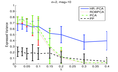
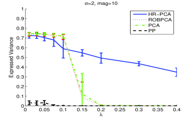
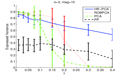
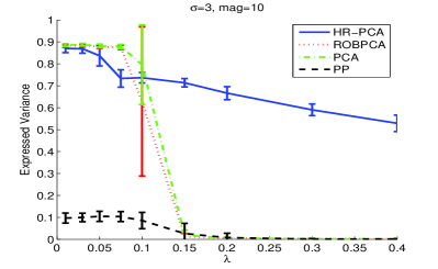
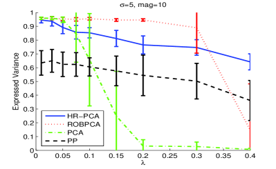
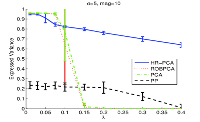
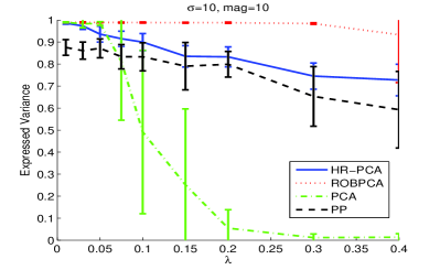
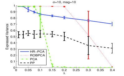
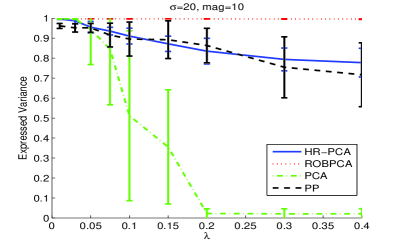
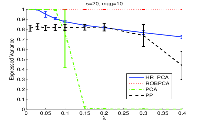
(a) $n=m=100$	(b) $n=m=1000$

Figure 2: Performance of HR-PCA vs ROBPCA, PP, PCA ($d=1$).

We make the following three observations from Figure 2. First, PP and ROBPCA can breakdown when $\lambda$ is large, while on the other hand, the performance of HR-PCA is rather robust even when $\lambda$ is as large as $40\%$. Second, the performance of PP and ROBPCA depends strongly on $\sigma$, i.e., the signal magnitude (and hence the magnitude of the corrupted points). Indeed, when $\sigma$ is very large, ROBPCA achieves effectively optimal recovery of the $A$ subspace. However, the performance of both algorithms is not satisfactory when $\sigma$ is small, and sometimes even worse than the performance of standard PCA. Finally, and perhaps most importantly, the performance of PP and ROBPCA degrades as the dimensionality increases, which makes them essentially not suitable for the high-dimensional regime we consider here. This is more explicitly shown in Figure 3 where the performance of different algorithms versus dimensionality is reported. We notice that the performance of ROBPCA (and similarly other algorithms based on Stahel-Donoho outlyingness) has a sharp decrease at a certain threshold that corresponds to the dimensionality where S-D outlyingness becomes invalid in identifying outliers.

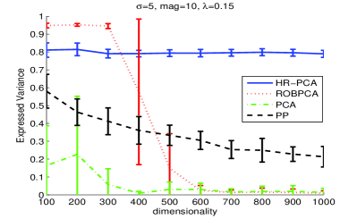
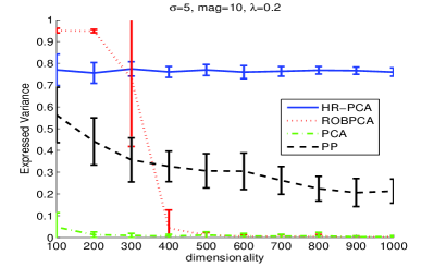
(a) $\lambda=0.15$	(b) $\lambda=0.2$
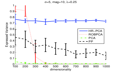
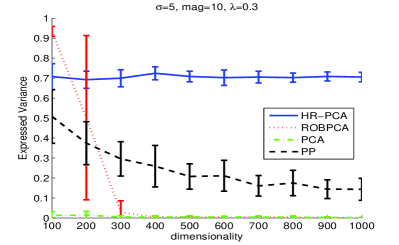
(c) $\lambda=0.25$	(d) $\lambda=0.3$

Figure 3: Performance vs dimensionality.

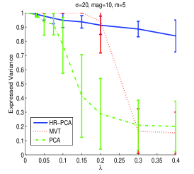
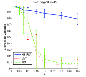
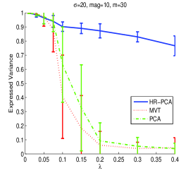
(a) $n=100,m=5$	(b) $n=100,m=15$	(c) $n=100,m=30$

Figure 4: Performance of HR-PCA vs MVT for $m\ll n$.

Figure 4 shows that the performance of MVT depends on the dimensionality $m$. Indeed, the breakdown property of MVT is roughly $1/m$ as predicted by the theoretical analysis, which makes MVT less attractive in the high-dimensional regime.

A similar numerical study for $d=3$ is also performed, where the outliers are generated on $3$ random chosen lines. The results are reported in Figure 5. The same trends as in the $d=1$ case are observed, although the performance gap between different strategies are smaller, because the effect of outliers are decreased since they are on $3$ directions.

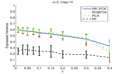
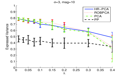
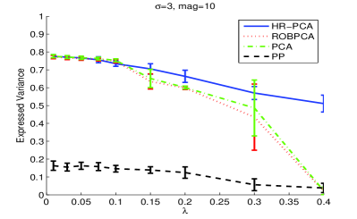
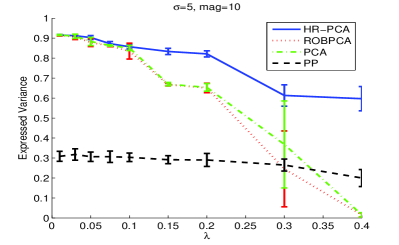
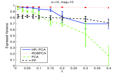
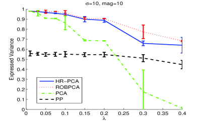
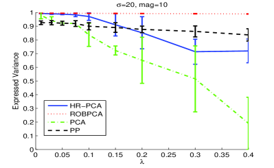
(a) $n=m=100$	(b) $n=m=1000$

Figure 5: Performance of HR-PCA vs ROBPCA, PP, PCA ($d=3$).

VII Concluding Remarks

In this paper, we investigated the dimensionality-reduction problem in the case where the number and the dimensionality of samples are of the same magnitude, and a constant fraction of the points are arbitrarily corrupted (perhaps maliciously so). We proposed a High-dimensional Robust Principal Component Analysis algorithm that is tractable, robust to corrupted points, easily kernelizable and asymptotically optimal. The algorithm iteratively finds a set of PCs using standard PCA and subsequently remove a point randomly with a probability proportional to its expressed variance. We provided both theoretical guarantees and favorable simulation results about the performance of the proposed algorithm.

To the best of our knowledge, previous efforts to extend existing robust PCA algorithms into the high-dimensional case remain unsuccessful. Such algorithms are designed for low dimensional data sets where the observations significantly outnumber the variables of each dimension. When applied to high-dimensional data sets, they either lose statistical consistency due to lack of sufficient observations, or become highly intractable. This motivates our work of proposing a new robust PCA algorithm that takes into account the inherent difficulty in analyzing high-dimensional data.

Appendix A The Details from Section V

In this appendix, we provide some of the details omitted in Section V.

A-A Proof of Lemma 2

Lemma 2 Given $\delta\in[0,1]$, $\hat{c}\in\mathbb{R}^{+}$, $\hat{m},m\in\mathbb{N}$ satisfying $\hat{m}<m$. Let $a_{1},\cdots,a_{m}$ be i.i.d. samples drawn from a probability measure $\mu$ supported on $\mathbb{R}^{+}$ and has a density function. Assume that $\mathbb{E}(a)=1$ and $\frac{1}{m}\sum_{i=1}^{m}a_{i}\leq 1+\hat{c}$. Then with probability at least $1-\delta$ we have

$$\sup_{\overline{m}\leq\hat{m}}|\frac{1}{m}\sum_{i=1}^{\overline{m}}a_{(i)}-\int_{0}^{\mu^{-1}({\overline{m}}/{m})}ad\mu|\leq\frac{(2+\hat{c})m}{m-\hat{m}}\sqrt{\frac{8(2\log m+1+\log\frac{8}{\delta})}{m}},$$

where $\mu^{-1}(x)\triangleq\min\{z|\mu(a\leq z)\geq x\}$.

Proof:

In Section V, using VC dimension argument, we showed that

$$\mathrm{Pr}\big{(}\sup_{e\geq 0}|\frac{1}{m}\sum_{i=1}^{m}g_{e}(a_{i})-\mathbb{E}g_{e}(a)|\geq\epsilon_{0}\big{)}\leq 4\exp(2\log m+1-m\epsilon_{0}^{2}/8)=\frac{\delta}{2};$$ (5)

and

$$\mathrm{Pr}\big{(}\sup_{e\in[0,(1+c)m/(m-\hat{m})]}|\frac{1}{m}\sum_{i=1}^{m}f_{e}(a_{i})-\mathbb{E}f_{e}(a)|\geq\epsilon\big{)}\leq 4\exp\left(2\log m+1-\frac{\epsilon^{2}(m-\hat{m})^{2}}{8(1+\hat{c})^{2}m}\right)=\frac{\delta}{2}.$$ (6)

To complete the proof, define $h(\cdot):[0,1]\rightarrow\mathbb{R}^{+}$ as $h(x)=\int_{0}^{\mu^{-1}(x)}ad\mu$. Since $\mu$ is supported on $\mathbb{R}^{+}$, by Markov inequality we have for any $n<m$,

$$a_{(n)}\leq a_{(n+1)}\leq\frac{(1+\hat{c})m}{m-n},$$

due to $\mathbb{E}(a)=1$ and $\frac{1}{m}\sum_{i=1}^{m}a_{i}\leq 1+\hat{c}$. Similarly, by Markov inequality we have for any $d,\epsilon\in[0,1]$ such that $d+\epsilon<1$, the following holds:

$$\frac{h(d+\epsilon)-h(d)}{(d+\epsilon)-d}\leq\frac{h(1)-h(d)}{1-d},$$

which implies

$$h(d+\epsilon)-h(d)\leq\frac{\epsilon}{1-d}.$$ (7)

Let $e_{n}=a_{(n)}$ for $n\leq m$, we have

$$\begin{split}&\sup_{\overline{m}\leq\hat{m}}\left|\frac{1}{m}\sum_{i=1}^{\overline{m}}a_{(i)}-h(\overline{m}/m)\right|\\ \leq&\sup_{\overline{m}\leq\hat{m}}\left\{\big{|}\frac{1}{m}\sum_{i=1}^{\overline{m}}a_{(i)}-\mathbb{E}f_{a_{(\overline{m})}}(a)\big{|}+\big{|}\mathbb{E}f_{a_{(\overline{m})}}(a)-h(\overline{m}/m)\big{|}\right\}\\ =&\sup_{\overline{m}\leq\hat{m}}\left\{\big{|}\frac{1}{m}\sum_{i=1}^{m}f_{e_{\overline{m}}}\big{(}a_{(i)}\big{)}-\mathbb{E}f_{e_{\overline{m}}}(a)\big{|}+\big{|}\mathbb{E}f_{e_{\overline{m}}}(a)-h(\overline{m}/m)\big{|}\right\}\\ \leq&\sup_{\overline{m}\leq\hat{m}}|\frac{1}{m}\sum_{i=1}^{m}f_{e_{\overline{m}}}(a_{(i)})-\mathbb{E}f_{e_{\overline{m}}}(a)|+\sup_{\overline{m}^{\prime}\leq\hat{m}}|\mathbb{E}f_{e_{\overline{m}^{\prime}}}(a)-h(\overline{m}^{\prime}/m)|.\end{split}$$

With probability at least $1-\delta/2$, the first term is upper bounded by $\epsilon$ due to Inequality (6). To bound the second term, we note that from Inequality (5), with probability at least $1-\delta/2$ the following holds

$$\sup_{\overline{m}^{\prime}\leq\hat{m}}\big{|}\overline{m}^{\prime}/m-\mu([0,e_{\overline{m}^{\prime}}])\big{|}=\sup_{\overline{m}^{\prime}\leq\hat{m}}\big{|}\frac{1}{m}\sum_{i=1}^{m}g_{e_{\overline{m}^{\prime}}}(a_{i})-\mathbb{E}g_{e_{\overline{m}^{\prime}}}(a)\big{|}\leq\epsilon_{0}.$$

This is equivalent to with probability $1-\gamma/2$, $\mu^{-1}(\overline{m}^{\prime}/m-\epsilon_{0})\leq e_{\overline{m}^{\prime}}\leq\mu^{-1}(\overline{m}^{\prime}/m+\epsilon_{0})$ holds uniformly for all $\overline{m}^{\prime}\leq\hat{m}$. Note that this further implies

$$\begin{split}&\sup_{\overline{m}^{\prime}\leq\hat{m}}|\mathbb{E}f_{e_{\overline{m}^{\prime}}}(a)-h(\overline{m}^{\prime}/m)|\\ \leq&\sup_{\overline{m}^{\prime}\leq\hat{m}}\max\big{[}h(\overline{m}^{\prime}/m+\epsilon_{0})-h(\overline{m}^{\prime}/m),h(\overline{m}^{\prime}/m))-h(\overline{m}^{\prime}/m-\epsilon_{0})\big{]}\\ \leq&\sup_{\overline{m}^{\prime}\leq\hat{m}}\frac{m\epsilon_{0}}{m-\overline{m}^{\prime}}=\frac{m\epsilon_{0}}{m-\hat{m}},\end{split}$$

where the last inequality follows from (A-A). This bounds the second term. Summing up the two terms proves the lemma. ∎

A-B Proof of Theorem 7

Theorem 7: If $\sup_{\mathbf{w}\in\mathcal{S}_{d}}\big{|}\frac{1}{t}\sum_{i=1}^{t}(\mathbf{w}^{\top}\mathbf{x}_{i})^{2}-1\big{|}\leq\hat{c}$, then

$$\begin{split}&\mathrm{Pr}\left\{\sup_{\mathbf{w}\in\mathcal{S}_{d},\overline{t}\leq\hat{t}}\big{|}\frac{1}{t}\sum_{i=1}^{\overline{t}}|\mathbf{w}^{\top}\mathbf{x}|_{(i)}^{2}-\mathcal{V}\left(\frac{\overline{t}}{t}\right)\big{|}\geq\epsilon\right\}\\ &\leq\max\left[\frac{8et^{2}6^{d}(1+\hat{c})^{d/2}}{\epsilon^{d/2}},\frac{8et^{2}24^{d}(1+\hat{c})^{d}t^{d/2}}{\epsilon^{d}(t-\hat{t})^{d/2}}\right]\exp\left(-\frac{\epsilon^{2}(1-\hat{t}/t)^{2}t}{32(2+\hat{c})^{2}}\right).\end{split}$$

Proof:

In Section V, we cover $\mathcal{S}_{d}$ with a finite $\epsilon$-net, and prove a uniform bound on this finite set, showing

$$\mathrm{Pr}\left\{\sup_{\mathbf{w}\in\hat{\mathcal{S}}_{d},\overline{t}\leq\hat{t}}\left|\frac{1}{t}\sum_{i=1}^{\overline{t}}|\mathbf{w}^{\top}\mathbf{x}|_{(i)}^{2}-\mathcal{V}\big{(}\frac{\overline{t}}{t}\big{)}\right|\geq\epsilon/2\right\}\leq\frac{8et^{2}3^{d}}{\delta^{d}}\exp\left(-\frac{(1-\hat{t}/t)^{2}\epsilon^{2}t}{32(2+\hat{c})^{2}}\right).$$

We have left to relate the uniform bound on $\mathcal{S}_{d}$ with the uniform bound on this finite set.

For any $\mathbf{w},\mathbf{w}_{1}\in\mathcal{S}_{d}$ such that $\|\mathbf{w}-\mathbf{w}_{1}\|\leq\delta$ and $\overline{t}\leq\hat{t}$, we have

$$\begin{split}&\big{|}\frac{1}{t}\sum_{i=1}^{\overline{t}}|{\mathbf{w}}^{\top}\mathbf{x}|_{(i)}^{2}-\frac{1}{t}\sum_{i=1}^{\hat{t}}|{\mathbf{w}_{1}}^{\top}\mathbf{x}|_{(i)}^{2}\big{|}\\ \leq&\max\Big{(}\big{|}\frac{1}{t}\sum_{i=1}^{\overline{t}}[(\mathbf{w}^{\top}\hat{\mathbf{x}}_{i})^{2}-(\mathbf{w}_{1}^{\top}\hat{\mathbf{x}}_{i})^{2}]\big{|},\,\big{|}\frac{1}{t}\sum_{i=1}^{\overline{t}}[(\mathbf{w}^{\top}\bar{\mathbf{x}}_{i})^{2}-(\mathbf{w}_{1}^{\top}\bar{\mathbf{x}}_{i})^{2}]\big{|}\Big{)},\end{split}$$ (8)

where $(\hat{\mathbf{x}}_{1},\cdots,\hat{\mathbf{x}}_{t})$ and $(\bar{\mathbf{x}}_{1},\cdots,\bar{\mathbf{x}}_{t})$ are permutations of $(\mathbf{x}_{1},\cdots,\mathbf{x}_{t})$ such that $|\mathbf{w}^{\top}\hat{\mathbf{x}}_{i}|$ and $|\mathbf{w}_{1}^{\top}\bar{\mathbf{x}}_{i}|$ are non-decreasing with $i$.

To bound the right hand side of (8), we note that

$$\begin{split}&\left|\frac{1}{t}\sum_{i=1}^{\overline{t}}[(\mathbf{w}^{\top}\hat{\mathbf{x}}_{i})^{2}-(\mathbf{w}_{1}^{\top}\hat{\mathbf{x}}_{i})^{2}]\right|=\left|\frac{1}{t}\sum_{i=1}^{\overline{t}}[(\mathbf{w}^{\top}\hat{\mathbf{x}}_{i})^{2}-((\mathbf{w}_{1}-\mathbf{w}+\mathbf{w})^{\top}\hat{\mathbf{x}}_{i})^{2}]\right|\\ =&\frac{1}{t}\left|-\sum_{i=1}^{\overline{t}}[(\mathbf{w}_{1}-\mathbf{w})^{\top}\hat{\mathbf{x}}_{i}]^{2}+2\sum_{i=1}^{\overline{t}}\big{\{}[(\mathbf{w}_{1}-\mathbf{w})^{\top}\hat{\mathbf{x}}_{i}][\mathbf{w}^{\top}\hat{\mathbf{x}}_{i}]\big{\}}\right|\\ \leq&\max_{\mathbf{v}\in\mathcal{S}_{d}}\delta^{2}\frac{1}{t}\sum_{i=1}^{\overline{t}}\mathbf{v}^{\top}\hat{\mathbf{x}}_{i}\hat{\mathbf{x}}_{i}^{\top}\mathbf{v}+2\delta\max_{\mathbf{v}^{\prime}\in\mathcal{S}_{d}}(\frac{1}{t}\sum_{i=1}^{\overline{t}}|\mathbf{v}^{\prime\top}\hat{\mathbf{x}}_{i}|)\cdot|\mathbf{w}^{\top}\hat{\mathbf{x}}_{\hat{t}}|.\end{split}$$ (9)

Here the inequality holds because $\|\mathbf{w}-\mathbf{w}_{1}\|\leq\delta$, and $|\mathbf{w}^{\top}\hat{\mathbf{x}}_{i}|$ is non-decreasing with $i$.

Note that for all $\mathbf{v},\mathbf{v}^{\prime}\in\mathcal{S}_{d}$, we have

$$\begin{split}(I)\quad&\max_{\mathbf{v}\in\mathcal{S}_{d}}\frac{1}{t}\sum_{i=1}^{\overline{t}}\mathbf{v}^{\top}\hat{\mathbf{x}}_{i}\hat{\mathbf{x}}_{i}^{\top}\mathbf{v}\leq\max_{\mathbf{v}\in\mathcal{S}_{d}}\frac{1}{t}\sum_{i=1}^{t}\mathbf{v}^{\top}\hat{\mathbf{x}}_{i}\hat{\mathbf{x}}_{i}^{\top}\mathbf{v}\leq 1+\hat{c};\\ (II)\quad&\frac{1}{t}\sum_{i=1}^{\overline{t}}|\mathbf{v}^{\prime\top}\hat{\mathbf{x}}_{i}|\leq\frac{1}{t}\sum_{i=1}^{t}|\mathbf{v}^{\prime\top}\hat{\mathbf{x}}_{i}|\leq\sqrt{\frac{1}{t}\sum_{i=1}^{t}|\mathbf{v}^{\prime\top}\hat{\mathbf{x}}_{i}|^{2}}\leq\sqrt{1+\hat{c}};\\ (III)\quad&\sum_{i=\hat{t}+1}^{t}|\mathbf{w}^{\top}\hat{\mathbf{x}}_{i}|^{2}\leq\sum_{i=1}^{t}|\mathbf{w}^{\top}\hat{\mathbf{x}}_{i}|^{2}\leq t(1+c);\quad\stackrel{{\scriptstyle(a)}}{{\Rightarrow}}\quad|\mathbf{w}^{\top}\hat{\mathbf{x}}_{\hat{t}}|\leq\sqrt{\frac{t(1+\hat{c})}{t-\hat{t}}}.\end{split}$$

Here, $(a)$ holds because $|\mathbf{w}^{\top}\hat{\mathbf{x}}_{i}|$ is non-decreasing with $i$. Substituting it back to the right hand side of (9) we have

$$\left|\frac{1}{t}\sum_{i=1}^{\overline{t}}[(\mathbf{w}^{\top}\hat{\mathbf{x}}_{i})^{2}-(\mathbf{w}_{1}^{\top}\hat{\mathbf{x}}_{i})^{2}]\right|\leq(1+\hat{c})\delta^{2}+2(1+\hat{c})\delta\sqrt{\frac{t}{t-\hat{t}}}\leq\epsilon/2.$$

Similarly we have

$$\begin{split}&\left|\frac{1}{t}\sum_{i=1}^{\overline{t}}\big{[}(\mathbf{w}^{\top}\bar{\mathbf{x}}_{i})^{2}-(\mathbf{w}_{1}^{\top}\bar{\mathbf{x}}_{i})^{2}\big{]}\right|=\left|\frac{1}{t}\sum_{i=1}^{\overline{t}}\big{[}((\mathbf{w}_{1}+\mathbf{w}-\mathbf{w}_{1})^{\top}\bar{\mathbf{x}}_{i})^{2}-(\mathbf{w}_{1}^{\top}\bar{\mathbf{x}}_{i})^{2}\big{]}\right|\\ =&\frac{1}{t}\left|\sum_{i=1}^{\overline{t}}[(\mathbf{w}-\mathbf{w}_{1})^{\top}\bar{\mathbf{x}}]^{2}-2\sum_{i=1}^{\overline{t}}\big{\{}[(\mathbf{w}^{\top}-\mathbf{w}_{1})^{\top}\bar{\mathbf{x}}_{i}][\mathbf{w}_{1}^{\top}\bar{\mathbf{x}}_{i}]\big{\}}\right|\\ \leq&\max_{\mathbf{v}\in\mathcal{S}_{d}}\delta^{2}\frac{1}{t}\sum_{i=1}^{\overline{t}}\mathbf{v}^{\top}\bar{\mathbf{x}}_{i}\bar{\mathbf{x}}_{i}^{\top}\mathbf{v}+2\delta\max_{\mathbf{v}^{\prime}\in\mathcal{S}_{d}}(\frac{1}{t}\sum_{i=1}^{\overline{t}}|\mathbf{v}^{\prime\top}\bar{\mathbf{x}}_{i}|)\cdot|\mathbf{w}_{1}^{\top}\bar{\mathbf{x}}_{\hat{t}}|,\end{split}$$

where the last inequality follows from that $|\mathbf{w}_{1}^{\top}\bar{\mathbf{x}}_{\hat{t}}|$ is non-decreasing with $i$. Note that the non-decreasing property also leads to

$$|\mathbf{w}_{1}^{\top}\bar{\mathbf{x}}_{\hat{t}}|\leq\sqrt{\frac{t(1+\hat{c})}{t-\hat{t}}},$$

which implies that

$$\big{|}\frac{1}{t}\sum_{i=1}^{\overline{t}}[(\mathbf{w}^{\top}\bar{\mathbf{x}}_{i})^{2}-(\mathbf{w}_{1}^{\top}\bar{\mathbf{x}}_{i})^{2}]\big{|}\leq\epsilon/2,$$

and consequently

$$\big{|}\frac{1}{t}\sum_{i=1}^{\overline{t}}|{\mathbf{w}}^{\top}\mathbf{x}|_{(i)}^{2}-\frac{1}{t}\sum_{i=1}^{\overline{t}}|{\mathbf{w}_{1}}^{\top}\mathbf{x}|_{(i)}^{2}\big{|}\leq\epsilon/2.$$

Thus,

$$\begin{split}&\mathrm{Pr}\left\{\sup_{\mathbf{w}\in\mathcal{S}_{d},\overline{t}\leq\hat{t}}\left|\frac{1}{t}\sum_{i=1}^{\overline{t}}|\mathbf{w}^{\top}\mathbf{x}|_{(i)}^{2}-\mathcal{V}\left(\frac{\overline{t}}{t}\right)\right|\geq\epsilon\right\}\\ \leq&\mathrm{Pr}\left\{\sup_{\mathbf{w}_{1}\in\hat{\mathcal{S}}_{d},\overline{t}\leq\hat{t}}\left|\frac{1}{t}\sum_{i=1}^{\overline{t}}|\mathbf{w}_{1}^{\top}\mathbf{x}|_{(i)}^{2}-\mathcal{V}\left(\frac{\overline{t}}{t}\right)\right|\geq\epsilon/2\right\}\\ \leq&8et^{2}\frac{3^{d}}{\delta^{d}}\exp\left(-\frac{\epsilon^{2}(1-\hat{t}/t)^{2}t}{32(2+\hat{c})^{2}}\right)\\ =&\max\left[8et^{2}\frac{3^{d}}{\delta_{1}^{d}}\exp\left(-\frac{\epsilon^{2}(1-\hat{t}/t)^{2}t}{32(2+\hat{c})^{2}}\right),\,8et^{2}\frac{3^{d}}{\delta_{2}^{d}}\exp\left(-\frac{\epsilon^{2}(1-\hat{t}/t)^{2}t}{32(2+\hat{c})^{2}}\right)\right]\\ =&\max\left[\frac{8e6^{d}(1+\hat{c})^{d/2}t^{2}}{\epsilon^{d/2}},\frac{8e24^{d}(1+\hat{c})^{d}t^{2}}{\epsilon^{d}(1-\hat{t}/t)^{d/2}}\right]\exp\left(-\frac{\epsilon^{2}(1-\hat{t}/t)^{2}t}{32(2+\hat{c})^{2}}\right).\end{split}$$

The first inequality holds because there exists $\mathbf{w}_{1}\in\hat{\mathcal{S}}_{d}$ such that $\|\mathbf{w}-\mathbf{w}_{1}\|\leq\delta$, which implies $\big{|}\frac{1}{t}\sum_{i=1}^{\overline{t}}|{\mathbf{w}}^{\top}\mathbf{x}|_{(i)}^{2}-\frac{1}{t}\sum_{i=1}^{\overline{t}}|{\mathbf{w}_{1}}^{\top}\mathbf{x}|_{(i)}^{2}\big{|}\leq\epsilon/2$.

∎

A-C Proof of Corollary 1 and Lemma 3

Corollary 1 If $\sup_{\mathbf{w}\in\mathcal{S}_{d}}\big{|}\frac{1}{t}\sum_{i=1}^{t}(\mathbf{w}^{\top}\mathbf{x}_{i})^{2}-1\big{|}\leq\hat{c}$, then with probability $1-\gamma$

$$\sup_{\mathbf{w}\in\mathcal{S}_{d},\overline{t}\leq\hat{t}}\big{|}\frac{1}{t}\sum_{i=1}^{\overline{t}}|\mathbf{w}^{\top}\mathbf{x}|_{(i)}^{2}-\mathcal{V}\left(\frac{\overline{t}}{t}\right)\big{|}\leq\epsilon_{0},$$

where

$$\begin{split}\epsilon_{0}=&\sqrt{\frac{32(2+\hat{c})^{2}\big{\{}\max[\frac{d+4}{2}\log t+\log{\frac{1}{\gamma}}+\log(16e6^{d})+\frac{d}{2}\log(1+\hat{c}),\,(1-\hat{t}/t)^{2}]\big{\}}}{t(1-\hat{t}/t)^{2}}}\\ &\,+\sqrt{\frac{32(2+\hat{c})^{2}\big{\{}\max[(d+2)\log t+\log{\frac{1}{\gamma}}+\log(16e^{2}24^{d})+d\log(1+\hat{c})-\frac{d}{2}\log(1-\hat{t}/t),\,(1-\hat{t}/t)^{2}]\big{\}}}{t(1-\hat{t}/t)^{2}}}.\end{split}$$

Proof:

The proof of the corollary requires Lemma 3.

Lemma 3 For any $C_{1},C_{2},d^{\prime},t\geq 0$, and $0<\gamma<1$. Let

$$\epsilon=\sqrt{\frac{\max(d^{\prime}\log t-\log(\gamma/C_{1}),C_{2})}{tC_{2}}},$$

then

$$C_{1}\epsilon^{-d^{\prime}}\exp(-C_{2}\epsilon^{2}t)\leq\gamma.$$

Proof:

Note that

$$\begin{split}&-C_{2}\epsilon^{2}t-d^{\prime}\log\epsilon\\ =&-\max(d^{\prime}\log t-\log(\gamma/C_{1}),C_{2})-d^{\prime}\log[\max(d^{\prime}\log t-\log(\gamma/C_{1})/C_{2},1)]+d^{\prime}\log t.\end{split}$$

It is easy to see that the r.h.s is upper-bounded by $\log(\gamma/C_{1})$ if $d^{\prime}\log t-\log(\gamma/C_{1})\geq C_{2}$. If $d^{\prime}\log t-\log(\gamma/C_{1})<C_{2}$, then the r.h.s equals $-C_{2}+d^{\prime}\log t$ which is again upper-bounded by $\log(\gamma/C_{1})$ due to $d^{\prime}\log t-\log(\gamma/C_{1})<C_{2}$. Thus, we have

$$-C_{2}\epsilon^{2}t-d^{\prime}\log\epsilon\leq\log(\gamma/C_{1}),$$

which is equivalent to

$$C_{1}\epsilon^{-d^{\prime}}\exp(-C_{2}\epsilon^{2}t)\leq\gamma.$$

∎

Now to prove the corollary: let

$$\begin{split}\epsilon_{1}&=\sqrt{\frac{32(2+\hat{c})^{2}\big{\{}\max[\frac{d+4}{2}\log t+\log{\frac{1}{\gamma}}+\log(16e6^{d})+\frac{d}{2}\log(1+\hat{c}),\,(1-\hat{t}/t)^{2}]\big{\}}}{t(1-\hat{t}/t)^{2}}}\\ \epsilon_{2}&=\sqrt{\frac{32(2+\hat{c})^{2}\big{\{}\max[(d+2)\log t+\log{\frac{1}{\gamma}}+\log(16e^{2}24^{d})+d\log(1+\hat{c})-\frac{d}{2}\log(1-\hat{t}/t),\,(1-\hat{t}/t)^{2}]\big{\}}}{t(1-\hat{t}/t)^{2}}}.\end{split}$$

By Lemma 3, we have

$$\begin{split}&\frac{8e6^{d}(1+\hat{c})^{d/2}t^{2}}{\epsilon_{1}^{d/2}}\exp\left(-\frac{\epsilon_{1}^{2}(1-\hat{t}/t)^{2}t}{32(2+\hat{c})^{2}}\right)\leq\gamma/2;\\ &\frac{8e24^{d}(1+\hat{c})^{d}t^{2}}{\epsilon_{2}^{d}(1-\hat{t}/t)^{d/2}}\exp\left(-\frac{\epsilon_{2}^{2}(1-\hat{t}/t)^{2}t}{32(2+\hat{c})^{2}}\right)\leq\gamma/2.\end{split}$$

By Theorem 7 we have

$$\begin{split}&\mathrm{Pr}\left\{\sup_{\mathbf{w}\in\mathcal{S}_{d},\overline{t}\leq\hat{t}}\big{|}\frac{1}{t}\sum_{i=1}^{\overline{t}}|\mathbf{w}^{\top}\mathbf{x}|_{(i)}^{2}-\mathcal{V}\left(\frac{\overline{t}}{t}\right)\big{|}\geq\epsilon_{0}\right\}\\ &\leq\max\left[\frac{8et^{2}6^{d}(1+\hat{c})^{d/2}}{\epsilon_{0}^{d/2}},\frac{8et^{2}24^{d}(1+\hat{c})^{d}t^{d/2}}{\epsilon_{0}^{d}(t-\hat{t})^{d/2}}\right]\exp\left(-\frac{\epsilon_{0}^{2}(1-\hat{t}/t)^{2}t}{32(2+\hat{c})^{2}}\right)\\ &\leq\left[\frac{8et^{2}6^{d}(1+\hat{c})^{d/2}}{\epsilon_{0}^{d/2}}+\frac{8et^{2}24^{d}(1+\hat{c})^{d}t^{d/2}}{\epsilon_{0}^{d}(t-\hat{t})^{d/2}}\right]\exp\left(-\frac{\epsilon_{0}^{2}(1-\hat{t}/t)^{2}t}{32(2+\hat{c})^{2}}\right)\\ &\leq\frac{8et^{2}6^{d}(1+\hat{c})^{d/2}}{\epsilon_{1}^{d/2}}\exp\left(-\frac{\epsilon_{1}^{2}(1-\hat{t}/t)^{2}t}{32(2+\hat{c})^{2}}\right)+\frac{8et^{2}24^{d}(1+\hat{c})^{d}t^{d/2}}{\epsilon_{2}^{d}(t-\hat{t})^{d/2}}\exp\left(-\frac{\epsilon_{2}^{2}(1-\hat{t}/t)^{2}t}{32(2+\hat{c})^{2}}\right)\\ &\leq\gamma.\end{split}$$

The third inequality holds because $\epsilon_{1},\epsilon_{2}\leq\epsilon_{0}$. ∎

A-D Proof of Theorem 9 and Lemma 4

Recall the statement of Theorem 9:

Theorem 9 With probability at least $1-\gamma$, $\bigcup_{s=1}^{s_{0}}\mathcal{E}(s)$ is true. Here

$$s_{0}\triangleq(1+\epsilon)\frac{(1+\kappa)\lambda n}{\kappa};\quad\epsilon=\frac{16(1+\kappa)\log(1/\gamma)}{\kappa\lambda n}+4\sqrt{\frac{(1+\kappa)\log(1/\gamma)}{\kappa\lambda n}}.$$

Recall that we defined the random variable $X_{s}$ as follows: Let $T=\min\{s|\mathcal{E}(s)\mbox{ is true}\}$. Note that since $\mathcal{E}(s)\in\mathcal{F}_{s-1}$, we have $\{T>s\}\in\mathcal{F}_{s-1}$. Then define:

$$X_{s}=\left\{\begin{array}[]{ll}|\mathcal{O}(T-1)|+\frac{\kappa(T-1)}{1+\kappa},&\mbox{if}\,\,T\leq s;\\ |\mathcal{O}(s)|+\frac{\kappa s}{1+\kappa},&\mbox{if}\,\,T>s.\end{array}\right.$$

The proof of the above theorem depends on first showing that the random variable, $X_{s}$, is a supermartingale.

Lemma 4. $\{X_{s},\mathcal{F}_{s}\}$ is a supermartingale.

Proof:

Observe that $X_{s}\in\mathcal{F}_{s}$. We next show that $\mathbb{E}(X_{s}|\mathcal{F}_{s-1})\leq X_{s-1}$ by enumerating the following three cases:

Case 1, $T>s$: Thus we have $\mathcal{E}^{c}(s)$ is true. By Lemma 10,

$$\mathbb{E}(X_{s}-X_{s-1}|\mathcal{F}_{s-1})=\mathbb{E}\left(\mathcal{O}(s)-\mathcal{O}(s-1)+\frac{\kappa}{1+\kappa}\Big{|}\mathcal{F}_{s-1}\right)=\frac{\kappa}{1+\kappa}-\mathrm{Pr}\left(\overline{r}(s)\in\mathcal{O}(s-1)\right)<0.$$

Case 2, $T=s$: By definition of $X_{s}$ we have $X_{s}=\mathcal{O}(s-1)+\kappa(s-1)/(1+\kappa)=X_{s-1}$.

Case 3, $T<s$: Since both $T$ and $s$ are integer, we have $T\leq s-1$. Thus, $X_{s-1}=\mathcal{O}(T-1)+\kappa(T-1)/(1+\kappa)=X_{s}$.

Combining all three cases shows that $\mathbb{E}(X_{s}|\mathcal{F}_{s-1})\leq X_{s-1}$, which proves the lemma. ∎

Next, we prove Theorem 9.

Proof:

Note that

$$\mathrm{Pr}\left(\bigcap_{s=1}^{s_{0}}\mathcal{E}(s)^{c}\right)=\mathrm{Pr}\left(T>s_{0}\right)\leq\mathrm{Pr}\left(X_{s_{0}}\geq\frac{\kappa s_{0}}{1+\kappa}\right)=\mathrm{Pr}\left(X_{s_{0}}\geq(1+\epsilon)\lambda n\right),$$ (10)

where the inequality is due to $|\mathcal{O}(s)|$ being non-negative.

Let $y_{s}\triangleq X_{s}-X_{s-1}$, where recall that $X_{0}=\lambda n$. Consider the following sequence:

$$y^{\prime}_{s}\triangleq y_{s}-\mathbb{E}(y_{s}|y_{1},\cdots,y_{s-1}).$$

Observe that $\{y^{\prime}_{s}\}$ is a martingale difference process w.r.t. $\{\mathcal{F}_{s}\}$. Since $\{X_{s}\}$ is a supermartingale, $\mathbb{E}(y_{s}|y_{1},\cdots,y_{s-1})\leq 0$ a.s. Therefore, the following holds a.s.,

$$X_{s}-X_{0}=\sum_{i=1}^{s}y_{i}=\sum_{i=1}^{s}y^{\prime}_{i}+\sum_{i=1}^{s}\mathbb{E}(y_{i}|y_{1},\cdots,y_{i-1})\leq\sum_{i=1}^{s}y^{\prime}_{i}.$$ (11)

By definition, $|y_{s}|\leq 1$, and hence $|y_{s}^{\prime}|\leq 2$. Now apply Azuma’s inequality

$$\begin{split}&\mathrm{Pr}(X_{s_{0}}\geq(1+\epsilon)\lambda n)\\ &\leq\mathrm{Pr}((\sum_{i=1}^{s_{0}}y^{\prime}_{i})\geq\epsilon\lambda n)\\ &\leq\exp(-(\epsilon\lambda n)^{2}/8s_{0})\\ &=\exp\left(-\frac{(\epsilon\lambda n)^{2}\kappa}{8(1+\epsilon)(1+\kappa)\lambda n}\right)\\ &\leq\exp\left(-\frac{(\epsilon\lambda n)^{2}\kappa}{8(1+\epsilon)(1+\kappa)\lambda n}\right)\\ &\leq\max\left(\exp\left(-\frac{\epsilon^{2}\lambda n\kappa}{16(1+\kappa)}\right),\,\exp\left(-\frac{\epsilon\lambda n\kappa}{16(1+\kappa)}\right)\right).\end{split}$$

We claim that the right-hand-side is upper bounded by $\gamma$. This is because:

$$\epsilon\geq\sqrt{\frac{16(1+\kappa)\log(1/\gamma)}{\kappa\lambda n}};\quad\Rightarrow\quad\exp\left(-\frac{\epsilon^{2}\lambda n\kappa}{16(1+\kappa)}\right)\leq\gamma;$$

and

$$\epsilon\geq\frac{16(1+\kappa)\log(1/\gamma)}{\kappa\lambda n};\quad\Rightarrow\quad\exp\left(-\frac{\epsilon\lambda n\kappa}{16(1+\kappa)}\right)\leq\gamma;$$

Substitute into (10), the theorem follows. ∎

A-E Proof of Lemmas 5 and 6 and Theorems 11 and 1

We now prove all the intermediate results used in Section V-F.

Lemma 5. If $\mathcal{E}(s)$ is true for some $s\leq s_{0}$, and there exists $\epsilon_{1},\epsilon_{2},\overline{c}$ such that

$$\begin{split}(I)\quad&\sup_{\mathbf{w}\in\mathcal{S}_{d}}\big{|}\frac{1}{t}\sum_{i=1}^{t-s_{0}}|\mathbf{w}^{\top}\mathbf{x}|_{(i)}^{2}-\mathcal{V}(\frac{t-s_{0}}{t})\big{|}\leq\epsilon_{1}\\ (II)\quad&\sup_{\mathbf{w}\in\mathcal{S}_{d}}\big{|}\frac{1}{t}\sum_{i=1}^{t}|\mathbf{w}^{\top}\mathbf{x}_{i}|^{2}-1\big{|}\leq\epsilon_{2}\\ (III)\quad&\sup_{\mathbf{w}\in\mathcal{S}_{m}}\frac{1}{t}\sum_{i=1}^{t}|\mathbf{w}^{\top}\mathbf{n}_{i}|^{2}\leq\overline{c},\end{split}$$

then

$$\frac{1}{1+\kappa}\left[(1-\epsilon_{1})\mathcal{V}\left(\frac{t-s_{0}}{t}\right)\overline{H}-2\sqrt{(1+\epsilon_{2})\overline{c}d\overline{H}}\right]\leq(1+\epsilon_{2})H_{s}+2\sqrt{(1+\epsilon_{2})\overline{c}dH_{s}}+\overline{c}.$$

Proof:

If $\mathcal{E}(s)$ is true, then we have

$$\sum_{j=1}^{d}\sum_{\mathbf{z}_{i}\in\mathcal{Z}(s-1)}(\mathbf{w}_{j}(s)^{\top}\mathbf{z}_{i})^{2}\geq\frac{1}{\kappa}\sum_{j=1}^{d}\sum_{\mathbf{o}_{i}\in\mathcal{O}(s-1)}(\mathbf{w}_{j}(s)^{\top}\mathbf{o}_{i})^{2}.$$

Recall that $\mathcal{Y}(s-1)=\mathcal{Z}(s-1)\bigcup\mathcal{O}(s-1)$, and that $\mathcal{Z}(s-1)$ and $\mathcal{O}(s-1)$ are disjoint. We thus have

$$\frac{1}{1+\kappa}\sum_{j=1}^{d}\sum_{\mathbf{y}_{i}\in\mathcal{Y}(s-1)}(\mathbf{w}_{j}(s)^{\top}\mathbf{y}_{i})^{2}\leq\sum_{j=1}^{d}\sum_{\mathbf{z}_{i}\in\mathcal{Z}(s-1)}(\mathbf{w}_{j}(s)^{\top}\mathbf{z}_{i})^{2}.$$ (12)

Since $\mathbf{w}_{1}(s),\cdots,\mathbf{w}_{d}(s)$ are the solution of the $s^{th}$ stage, the following holds by definition of the algorithm

$$\sum_{j=1}^{d}\sum_{\mathbf{y}_{i}\in\mathcal{Y}(s-1)}(\overline{\mathbf{w}}_{j}^{\top}\mathbf{y}_{i})^{2}\leq\sum_{j=1}^{d}\sum_{\mathbf{y}_{i}\in\mathcal{Y}(s-1)}(\mathbf{w}_{j}(s)^{\top}\mathbf{y}_{i})^{2}.$$ (13)

Further note that by $\mathcal{Z}(s-1)\subseteq\mathcal{Y}(s-1)$ and $\mathcal{Z}(s-1)\subseteq\mathcal{Z}$, we have

$$\sum_{j=1}^{d}\sum_{\mathbf{z}_{i}\in\mathcal{Z}(s-1)}(\overline{\mathbf{w}}_{j}^{\top}\mathbf{z}_{i})^{2}\leq\sum_{j=1}^{d}\sum_{\mathbf{y}_{i}\in\mathcal{Y}(s-1)}(\overline{\mathbf{w}}_{j}^{\top}\mathbf{y}_{i})^{2},$$

and

$$\sum_{j=1}^{d}\sum_{\mathbf{z}_{i}\in\mathcal{Z}(s-1)}(\mathbf{w}_{j}(s)^{\top}\mathbf{z}_{i})^{2}\leq\sum_{j=1}^{d}\sum_{\mathbf{z}_{i}\in\mathcal{Z}}(\mathbf{w}_{j}(s)^{\top}\mathbf{z}_{i})^{2}=\sum_{j=1}^{d}\sum_{i=1}^{t}(\mathbf{w}_{j}(s)^{\top}\mathbf{z}_{i})^{2}.$$

Substituting them into (12) and  (13) we have

$$\frac{1}{1+\kappa}\sum_{j=1}^{d}\sum_{\mathbf{z}_{i}\in\mathcal{Z}(s-1)}(\overline{\mathbf{w}}_{j}^{\top}\mathbf{z}_{i})^{2}\leq\sum_{j=1}^{d}\sum_{i=1}^{t}(\mathbf{w}_{j}(s)^{\top}\mathbf{z}_{i})^{2}.$$

Note that $|\mathcal{Z}(s-1)|\geq t-(s-1)\geq t-s_{0}$, hence for all $j=1,\cdots,d$,

$$\begin{split}&\sum_{i=1}^{t-s_{0}}\big{|}\overline{\mathbf{w}}_{j}\mathbf{z}\big{|}_{(i)}^{2}\leq\sum_{i=1}^{|\mathcal{Z}(s-1)|}\big{|}\overline{\mathbf{w}}_{j}\mathbf{z}\big{|}_{(i)}^{2}\leq\sum_{\mathbf{z}_{i}\in\mathcal{Z}(s-1)}(\overline{\mathbf{w}}_{j}\mathbf{z}_{i})^{2},\end{split}$$

which in turn implies

$$\frac{1}{1+\kappa}\sum_{i=1}^{t-s_{0}}\big{|}\overline{\mathbf{w}}_{j}\mathbf{z}\big{|}_{(i)}^{2}\leq\sum_{j=1}^{d}\sum_{i=1}^{t}(\mathbf{w}_{j}(s)^{\top}\mathbf{z}_{i})^{2}.$$

By Corollary 2 and Corollary 3 we conclude

$$\frac{1}{1+\kappa}\left[(1-\epsilon_{1})\mathcal{V}\left(\frac{t-s_{0}}{t}\right)\overline{H}-2\sqrt{(1+\epsilon_{2})\overline{c}d\overline{H}}\right]\leq(1+\epsilon_{2})H_{s}+2\sqrt{(1+\epsilon_{2})\overline{c}dH_{s}}+\overline{c}.$$

∎

Lemma 6. Fix a $\hat{t}\leq t$. If $\sum_{j=1}^{d}\overline{V}_{\hat{t}}(\mathbf{w}_{j})\geq\sum_{j=1}^{d}\overline{V}_{\hat{t}}(\mathbf{w}^{\prime}_{j})$, and there exists $\epsilon_{1},\epsilon_{2},\overline{c}$ such that

$$\begin{split}(I)\quad&\sup_{\mathbf{w}\in\mathcal{S}_{d}}\big{|}\frac{1}{t}\sum_{i=1}^{\hat{t}}|\mathbf{w}^{\top}\mathbf{x}|_{(i)}^{2}-\mathcal{V}(\frac{\hat{t}}{t})\big{|}\leq\epsilon_{1},\\ (II)\quad&\sup_{\mathbf{w}\in\mathcal{S}_{d}}\big{|}\frac{1}{t}\sum_{i=1}^{\hat{t}-\frac{\lambda t}{1-\lambda}}|\mathbf{w}^{\top}\mathbf{x}|_{(i)}^{2}-\mathcal{V}\left(\frac{\hat{t}}{t}-\frac{\lambda}{1-\lambda}\right)\big{|}\leq\epsilon_{1},\\ (III)\quad&\sup_{\mathbf{w}\in\mathcal{S}_{d}}\big{|}\frac{1}{t}\sum_{i=1}^{t}|\mathbf{w}^{\top}\mathbf{x}_{i}|^{2}-1\big{|}\leq\epsilon_{2},\\ (IV)\quad&\sup_{\mathbf{w}\in\mathcal{S}_{m}}\frac{1}{t}\sum_{i=1}^{t}|\mathbf{w}^{\top}\mathbf{n}_{i}|^{2}\leq\overline{c},\end{split}$$

then

$$\begin{split}&(1-\epsilon_{1})\mathcal{V}\left(\frac{\hat{t}}{t}-\frac{\lambda}{1-\lambda}\right)H(\mathbf{w}_{1}^{\prime}\cdots,\mathbf{w}_{d}^{\prime})-2\sqrt{(1+\epsilon_{2})\overline{c}dH(\mathbf{w}_{1}^{\prime}\cdots,\mathbf{w}_{d}^{\prime})}\\ \leq&(1+\epsilon_{1})H(\mathbf{w}_{1}\cdots,\mathbf{w}_{d})\mathcal{V}\left(\frac{\hat{t}}{t}\right)+2\sqrt{(1+\epsilon_{2})\overline{c}dH(\mathbf{w}_{1}\cdots,\mathbf{w}_{d})}+\overline{c}.\end{split}$$

Proof:

Recall that $\overline{V}_{\hat{t}}(\mathbf{w})=\frac{1}{n}\sum_{i=1}^{\hat{t}}|\mathbf{w}^{\top}\mathbf{y}|_{(i)}^{2}$. Since $\mathcal{Y}\subset\mathcal{Z}$ and $|\mathcal{Z}\backslash\mathcal{Y}|=\lambda n=\lambda t/(1-\lambda)$, we have

$$\sum_{i=1}^{\hat{t}-\frac{\lambda t}{1-\lambda}}|\mathbf{w}^{\top}\mathbf{z}|_{(i)}^{2}\leq\sum_{i=1}^{\hat{t}}|\mathbf{w}^{\top}\mathbf{y}|_{(i)}^{2}\leq\sum_{i=1}^{\hat{t}}|\mathbf{w}^{\top}\mathbf{z}|_{(i)}^{2}.$$

By assumption $\sum_{j=1}^{d}\overline{V}_{\hat{t}}(\mathbf{w}_{j})\geq\sum_{j=1}^{d}\overline{V}_{\hat{t}}(\mathbf{w}^{\prime}_{j})$, we have

$$\sum_{j=1}^{d}\sum_{i=1}^{\hat{t}-\frac{\lambda t}{1-\lambda}}|\mathbf{w}_{j}^{\prime\top}\mathbf{y}|_{(i)}^{2}\leq\sum_{j=1}^{d}\sum_{i=1}^{\hat{t}}|\mathbf{w}_{j}^{\top}\mathbf{y}|_{(i)}^{2}.$$

By Corollary 2 and Corollary 3 we conclude

$$\begin{split}&(1-\epsilon_{1})\mathcal{V}\left(\frac{\hat{t}}{t}-\frac{\lambda}{1-\lambda}\right)H(\mathbf{w}_{1}^{\prime}\cdots,\mathbf{w}_{d}^{\prime})-2\sqrt{(1+\epsilon_{2})\overline{c}dH(\mathbf{w}_{1}^{\prime}\cdots,\mathbf{w}_{d}^{\prime})}\\ \leq&(1+\epsilon_{1})H(\mathbf{w}_{1}\cdots,\mathbf{w}_{d})\mathcal{V}\left(\frac{\hat{t}}{t}\right)+2\sqrt{(1+\epsilon_{2})\overline{c}dH(\mathbf{w}_{1}\cdots,\mathbf{w}_{d})}+\overline{c}.\end{split}$$

∎

Theorem 11. If $\bigcup_{s=1}^{s_{0}}\mathcal{E}(s)$ is true, and there exists $\epsilon_{1}<1,\epsilon_{2},\overline{c}$ such that

$$\begin{split}(I)\quad&\sup_{\mathbf{w}\in\mathcal{S}_{d}}\big{|}\frac{1}{t}\sum_{i=1}^{t-s_{0}}|\mathbf{w}^{\top}\mathbf{x}|_{(i)}^{2}-\mathcal{V}(\frac{t-s_{0}}{t})\big{|}\leq\epsilon_{1}\\ (II)\quad&\sup_{\mathbf{w}\in\mathcal{S}_{d}}\big{|}\frac{1}{t}\sum_{i=1}^{\hat{t}}|\mathbf{w}^{\top}\mathbf{x}|_{(i)}^{2}-\mathcal{V}(\frac{\hat{t}}{t})\big{|}\leq\epsilon_{1}\\ (III)\quad&\sup_{\mathbf{w}\in\mathcal{S}_{d}}\big{|}\frac{1}{t}\sum_{i=1}^{\hat{t}-\frac{\lambda t}{1-\lambda}}|\mathbf{w}^{\top}\mathbf{x}|_{(i)}^{2}-\mathcal{V}\left(\frac{\hat{t}}{t}-\frac{\lambda}{1-\lambda}\right)\big{|}\leq\epsilon_{1}\\ (IV)\quad&\sup_{\mathbf{w}\in\mathcal{S}_{d}}\big{|}\frac{1}{t}\sum_{i=1}^{t}|\mathbf{w}^{\top}\mathbf{x}_{i}|^{2}-1\big{|}\leq\epsilon_{2}\\ (V)\quad&\sup_{\mathbf{w}\in\mathcal{S}_{m}}\frac{1}{t}\sum_{i=1}^{t}|\mathbf{w}^{\top}\mathbf{n}_{i}|^{2}\leq\overline{c},\end{split}$$

then

$$\begin{split}&\frac{H^{*}}{\overline{H}}\geq\frac{(1-\epsilon_{1})^{2}\mathcal{V}\left(\frac{\hat{t}}{t}-\frac{\lambda}{1-\lambda}\right)\mathcal{V}\left(\frac{t-s_{0}}{t}\right)}{(1+\epsilon_{1})(1+\epsilon_{2})(1+\kappa)\mathcal{V}\left(\frac{\hat{t}}{t}\right)}\\ &\quad-\left[\frac{(2\kappa+4)(1-\epsilon_{1})\mathcal{V}\left(\frac{\hat{t}}{t}-\frac{\lambda}{1-\lambda}\right)\sqrt{(1+\epsilon_{2})\overline{c}d}+4(1+\kappa)(1+\epsilon_{2})\sqrt{(1+\epsilon_{2})\overline{c}d}}{(1+\epsilon_{1})(1+\epsilon_{2})(1+\kappa)\mathcal{V}\left(\frac{\hat{t}}{t}\right)}\right](\overline{H})^{-1/2}\\ &\quad-\left[\frac{(1-\epsilon_{1})\mathcal{V}\left(\frac{\hat{t}}{t}-\frac{\lambda}{1-\lambda}\right)\overline{c}+(1+\epsilon_{2})\overline{c}}{(1+\epsilon_{1})(1+\epsilon_{2})\mathcal{V}\left(\frac{\hat{t}}{t}\right)}\right](\overline{H})^{-1}.\end{split}$$ (14)

Proof:

Since $\bigcup_{s=1}^{s_{0}}\mathcal{E}(s)$ is true, there exists a $s^{\prime}\leq s_{0}$ such that $\mathcal{E}(s^{\prime})$ is true. By Lemma 5 we have

$$\frac{1}{1+\kappa}\left[(1-\epsilon_{1})\mathcal{V}\left(\frac{t-s_{0}}{t}\right)\overline{H}-2\sqrt{(1+\epsilon_{2})\overline{c}d\overline{H}}\right]\leq(1+\epsilon_{2})H_{s^{\prime}}+2\sqrt{(1+\epsilon_{2})\overline{c}dH_{s^{\prime}}}+\overline{c}.$$

By the definition of the algorithm, we have $\sum_{j=1}^{d}\overline{V}_{\hat{t}}(\mathbf{w}^{*}_{j})\geq\sum_{j=1}^{d}\overline{V}_{\hat{t}}(\mathbf{w}_{j}(s^{\prime}))$, which by Lemma 6 implies

$$\begin{split}&(1-\epsilon_{1})\mathcal{V}\left(\frac{\hat{t}}{t}-\frac{\lambda}{1-\lambda}\right)H_{s^{\prime}}-2\sqrt{(1+\epsilon_{2})\overline{c}dH_{s^{\prime}}}\leq(1+\epsilon_{1})H^{*}\mathcal{V}\left(\frac{\hat{t}}{t}\right)+2\sqrt{(1+\epsilon_{2})\overline{c}dH^{*}}+\overline{c}.\end{split}$$

By definition, $H_{s^{\prime}},H^{*}\leq\overline{H}$. Thus we have

$$\begin{split}(I)\quad&\frac{1}{1+\kappa}\left[(1-\epsilon_{1})\mathcal{V}\left(\frac{t-s_{0}}{t}\right)\overline{H}-2\sqrt{(1+\epsilon_{2})\overline{c}d\overline{H}}\right]\leq(1+\epsilon_{2})H_{s^{\prime}}+2\sqrt{(1+\epsilon_{2})\overline{c}d\overline{H}}+\overline{c};\\ (II)\quad&(1-\epsilon_{1})\mathcal{V}\left(\frac{\hat{t}}{t}-\frac{\lambda}{1-\lambda}\right)H_{s^{\prime}}-2\sqrt{(1+\epsilon_{2})\overline{c}d\overline{H}}\leq(1+\epsilon_{1})\mathcal{V}\left(\frac{\hat{t}}{t}\right)H^{*}+2\sqrt{(1+\epsilon_{2})\overline{c}d\overline{H}}+\overline{c}.\end{split}$$

Rearrange the inequalities, we have

$$\begin{split}&(I)\quad(1-\epsilon_{1})\mathcal{V}\big{(}\frac{t-s_{0}}{t}\big{)}\overline{H}-(2\kappa+4)\sqrt{(1+\epsilon_{2})\overline{c}d\overline{H}}-(1+\kappa)\overline{c}\leq(1+\kappa)(1+\epsilon_{2})H_{s^{\prime}};\\ &(II)\quad(1-\epsilon_{1})\mathcal{V}\left(\frac{\hat{t}}{t}-\frac{\lambda}{1-\lambda}\right)H_{s^{\prime}}\leq(1+\epsilon_{1})\mathcal{V}\left(\frac{\hat{t}}{t}\right)H^{*}+4\sqrt{(1+\epsilon_{2})\overline{c}d\overline{H}}+\overline{c}.\end{split}$$

Simplify the inequality. We get

$$\begin{split}&\frac{H^{*}}{\overline{H}}\geq\frac{(1-\epsilon_{1})^{2}\mathcal{V}\left(\frac{\hat{t}}{t}-\frac{\lambda}{1-\lambda}\right)\mathcal{V}\left(\frac{t-s_{0}}{t}\right)}{(1+\epsilon_{1})(1+\epsilon_{2})(1+\kappa)\mathcal{V}\left(\frac{\hat{t}}{t}\right)}\\ &\quad-\left[\frac{(2\kappa+4)(1-\epsilon_{1})\mathcal{V}\left(\frac{\hat{t}}{t}-\frac{\lambda}{1-\lambda}\right)\sqrt{(1+\epsilon_{2})\overline{c}d}+4(1+\kappa)(1+\epsilon_{2})\sqrt{(1+\epsilon_{2})\overline{c}d}}{(1+\epsilon_{1})(1+\epsilon_{2})(1+\kappa)\mathcal{V}\left(\frac{\hat{t}}{t}\right)}\right](\overline{H})^{-1/2}\\ &\quad-\left[\frac{(1-\epsilon_{1})\mathcal{V}\left(\frac{\hat{t}}{t}-\frac{\lambda}{1-\lambda}\right)\overline{c}+(1+\epsilon_{2})\overline{c}}{(1+\epsilon_{1})(1+\epsilon_{2})\mathcal{V}\left(\frac{\hat{t}}{t}\right)}\right](\overline{H})^{-1}.\end{split}$$

∎

Theorem 1. Let $\tau=\max(m/n,1)$. There exists a universal constant $c_{0}$ and a constant $C$ which can possible depend on $\hat{t}/t$, $\lambda$, $d$, $\mu$ and $\kappa$, such that for any $\gamma<1$, if $n/\log^{4}n\geq\log^{6}(1/\gamma)$, then with probability $1-\gamma$ the following holds

$$\begin{split}\frac{H^{*}}{\overline{H}}\geq\frac{\mathcal{V}\left(\frac{\hat{t}}{t}-\frac{\lambda}{1-\lambda}\right)\mathcal{V}\left(1-\frac{\lambda(1+\kappa)}{(1-\lambda)\kappa}\right)}{(1+\kappa)\mathcal{V}\left(\frac{\hat{t}}{t}\right)}-\left[\frac{8\sqrt{c_{0}\tau d}}{\mathcal{V}\left(\frac{\hat{t}}{t}\right)}\right](\overline{H})^{-1/2}-\left[\frac{2c_{0}\tau}{\mathcal{V}\left(\frac{\hat{t}}{t}\right)}\right](\overline{H})^{-1}-C\frac{\log^{2}n\log^{3}(1/\gamma)}{\sqrt{n}}.\end{split}$$

Proof:

We need to bound all diminishing terms in the r.h.s. of (LABEL:equ.step6noprobability). We need to lower bound $\mathcal{V}((t-s_{0})/{t})$ using the following lemma.

Lemma 7

$$\mathcal{V}\left(\frac{t-s_{0}}{t}\right)\geq\mathcal{V}\left(1-\frac{\lambda(1+\kappa)}{(1-\lambda)\kappa}\right)-\epsilon,$$

where $\epsilon\leq c\frac{\log(1/\gamma)}{n}+c\sqrt{\frac{\log(1/\gamma)}{n}}$.

Proof:

Given $a^{-}<a^{+}<1$, by the definition of $\mathcal{V}$ we have

$$\frac{\mathcal{V}(a^{+})-\mathcal{V}(a^{-})}{a^{+}-a^{-}}\leq\frac{1-\mathcal{V}(a^{+})}{1-a^{+}}.$$

Re-arranging, we have

$$\mathcal{V}(a^{-})\geq\frac{1-a^{-}}{1-a^{+}}\mathcal{V}(a^{+})-\frac{a^{+}-a^{-}}{1-a^{+}}\geq\mathcal{V}(a^{+})-\frac{a^{+}-a^{-}}{1-a^{+}}.$$

Recall $s_{0}=(1+\epsilon)(1+\kappa)\lambda n/\kappa=(1+\epsilon)(1+\kappa)\lambda t/(\kappa(1-\lambda))$. Let $s^{\prime}=(1+\kappa)\lambda t/(\kappa(1-\lambda))$. Take $a^{+}=t-s^{\prime}$, and $a^{-}=t-s_{0}$, the lemma follows. ∎

We also need the following two lemmas. The proofs are straightforward.

Lemma 8

For any $0\leq\alpha_{1},\alpha_{2}\leq 1$ and $c>0$, we have

$$1-\alpha\leq 1/(1+\alpha);\quad(1-\alpha_{1})(1-\alpha_{2})\leq 1-(\alpha_{1}+\alpha_{2});\quad\sqrt{c+\alpha_{1}}\leq\sqrt{c}+\alpha_{1}.$$

Lemma 9

If $n/\log^{4}n\geq\log^{6}(1/\gamma)$, then

$$\max\left(\frac{\log(1/\gamma)}{n},\sqrt{\frac{\log n}{n}},\sqrt{\frac{\log(1/\gamma)}{n}},\frac{\log^{2.5}n\log^{3.5}(1/\gamma)}{n}\right)\leq\frac{\log^{2}n\log^{3}(1/\gamma)}{\sqrt{n}}\leq 1.$$

Recall that with probability $1-\gamma$, $\overline{c}\leq c_{0}\tau+c\frac{\log(1/\gamma)}{n}$ where $c_{0}$ is a universal constant, and the constant $c$ depends on $\kappa$, $\hat{t}/t$, $\lambda$, $d$ and $\mu$. We denote $\overline{c}-c_{0}\tau$ by $\epsilon_{c}$. Iteratively applying Lemma 8, we have the following holds when $\epsilon_{1},\epsilon_{2},\epsilon_{c}<1$,

$$\begin{split}&\frac{H^{*}}{\overline{H}}\geq\frac{(1-\epsilon_{1})^{2}\mathcal{V}\left(\frac{\hat{t}}{t}-\frac{\lambda}{1-\lambda}\right)\mathcal{V}\left(\frac{t-s_{0}}{t}\right)}{(1+\epsilon_{1})(1+\epsilon_{2})(1+\kappa)\mathcal{V}\left(\frac{\hat{t}}{t}\right)}\\ &\quad-\left[\frac{(2\kappa+4)(1-\epsilon_{1})\mathcal{V}\left(\frac{\hat{t}}{t}-\frac{\lambda}{1-\lambda}\right)\sqrt{(1+\epsilon_{2})\overline{c}d}+4(1+\kappa)(1+\epsilon_{2})\sqrt{(1+\epsilon_{2})\overline{c}d}}{(1+\epsilon_{1})(1+\epsilon_{2})(1+\kappa)\mathcal{V}\left(\frac{\hat{t}}{t}\right)}\right](\overline{H})^{-1/2}\\ &\quad-\left[\frac{(1-\epsilon_{1})\mathcal{V}\left(\frac{\hat{t}}{t}-\frac{\lambda}{1-\lambda}\right)\overline{c}+(1+\epsilon_{2})\overline{c}}{(1+\epsilon_{1})(1+\epsilon_{2})\mathcal{V}\left(\frac{\hat{t}}{t}\right)}\right](\overline{H})^{-1}\\ &\geq\frac{(1-\epsilon_{1})^{2}\mathcal{V}\left(\frac{\hat{t}}{t}-\frac{\lambda}{1-\lambda}\right)\mathcal{V}\left(\frac{t-s^{\prime}}{t}\right)}{(1+\epsilon_{1})(1+\epsilon_{2})(1+\kappa)\mathcal{V}\left(\frac{\hat{t}}{t}\right)}-\epsilon-\left[\frac{4\sqrt{\overline{c}d}+4\sqrt{(1+\epsilon_{2})\overline{c}d}}{\mathcal{V}\left(\frac{\hat{t}}{t}\right)}\right](\overline{H})^{-1/2}-\left[\frac{2\overline{c}}{\mathcal{V}\left(\frac{\hat{t}}{t}\right)}\right](\overline{H})^{-1}\\ &\geq\frac{(1-\epsilon_{1})^{3}(1-\epsilon_{2})\mathcal{V}\left(\frac{\hat{t}}{t}-\frac{\lambda}{1-\lambda}\right)\mathcal{V}\left(\frac{t-s^{\prime}}{t}\right)}{(1+\kappa)\mathcal{V}\left(\frac{\hat{t}}{t}\right)}-\epsilon-\left[\frac{4\sqrt{\overline{c}d}+4\sqrt{(1+\epsilon_{2})\overline{c}d}}{\mathcal{V}\left(\frac{\hat{t}}{t}\right)}\right](\overline{H})^{-1/2}-\left[\frac{2\overline{c}}{\mathcal{V}\left(\frac{\hat{t}}{t}\right)}\right](\overline{H})^{-1}\\ &\geq\frac{(1-15\max(\epsilon_{1},\,\epsilon_{2}))\mathcal{V}\left(\frac{\hat{t}}{t}-\frac{\lambda}{1-\lambda}\right)\mathcal{V}\left(\frac{t-s^{\prime}}{t}\right)}{(1+\kappa)\mathcal{V}\left(\frac{\hat{t}}{t}\right)}-\epsilon\\ &\quad-\left[\frac{4\sqrt{(c_{0}\tau+\epsilon_{c})d}+4(1+\epsilon_{2})\sqrt{(c_{0}\tau+\epsilon_{c})d}}{\mathcal{V}\left(\frac{\hat{t}}{t}\right)}\right](\overline{H})^{-1/2}-\left[\frac{2(c_{0}\tau+\epsilon_{c})}{\mathcal{V}\left(\frac{\hat{t}}{t}\right)}\right](\overline{H})^{-1}\\ &\geq\frac{(1-15\max(\epsilon_{1},\,\epsilon_{2}))\mathcal{V}\left(\frac{\hat{t}}{t}-\frac{\lambda}{1-\lambda}\right)\mathcal{V}\left(\frac{t-s^{\prime}}{t}\right)}{(1+\kappa)\mathcal{V}\left(\frac{\hat{t}}{t}\right)}-\epsilon\\ &\quad-\left[\frac{4(\sqrt{c_{0}\tau}+\epsilon_{c})\sqrt{d}+4(1+\epsilon_{2})(\sqrt{c_{0}\tau}+\epsilon_{c})\sqrt{d}}{\mathcal{V}\left(\frac{\hat{t}}{t}\right)}\right](\overline{H})^{-1/2}-\left[\frac{2(c_{0}\tau+\epsilon_{c})}{\mathcal{V}\left(\frac{\hat{t}}{t}\right)}\right](\overline{H})^{-1}.\end{split}$$

Recall that with probability $1-\gamma$, $\epsilon_{2}\leq c\frac{\log^{2}n\log^{3}{1/\gamma}}{\sqrt{n}}$, $\epsilon\leq c\frac{\log(1/\gamma)}{n}+c\sqrt{\frac{\log(1/\gamma)}{n}}$, $\overline{c}\leq c_{0}\tau+c\frac{\log(1/\gamma)}{n}$. Furthermore, $\epsilon_{1}\leq c\sqrt{\frac{\log n+\log(1/\gamma)}{n}}+c\frac{\log^{2.5}n\log^{3.5}(1/\gamma)}{n}$ if $\hat{t}/t=\eta<1$, and $\epsilon_{1}\leq\max(c\sqrt{\frac{\log n+\log(1/\gamma)}{n}}+c\frac{\log^{2.5}n\log^{3.5}(1/\gamma)}{n},\epsilon_{2})$ if $\hat{t}=t$. Here, $c_{0}$ is a universal constant, and the constant $c$ depends on $\kappa$, $\eta$, $\lambda$, $d$ and $\mu$. Further note by Lemma 9 we can bound all diminishing terms by $\frac{\log^{2}n\log^{3}(1/\gamma)}{\sqrt{n}}$. Therefore, we have when $\epsilon_{1},\epsilon_{2},\epsilon_{c}<1$,

$$\begin{split}\frac{H^{*}}{\overline{H}}\geq\frac{\mathcal{V}\left(\frac{\hat{t}}{t}-\frac{\lambda}{1-\lambda}\right)\mathcal{V}\left(1-\frac{\lambda(1+\kappa)}{(1-\lambda)\kappa}\right)}{(1+\kappa)\mathcal{V}\left(\frac{\hat{t}}{t}\right)}-\left[\frac{8\sqrt{c_{0}\tau d}}{\mathcal{V}\left(\frac{\hat{t}}{t}\right)}\right](\overline{H})^{-1/2}-\left[\frac{2c_{0}\tau}{\mathcal{V}\left(\frac{\hat{t}}{t}\right)}\right](\overline{H})^{-1}-C_{1}\frac{\log^{2}n\log^{3}(1/\gamma)}{\sqrt{n}}.\end{split}$$

On the other hand, when $\max(\epsilon_{1},\epsilon_{2},\epsilon_{c})\geq 1$, since by Lemma 9, $\max(\epsilon_{1},\epsilon_{2},\epsilon_{c})\leq C_{2}\frac{\log^{2}n\log^{3}(1/\gamma)}{\sqrt{n}}$ for some constant $C_{2}$. Thus, $C_{2}\frac{\log^{2}n\log^{3}(1/\gamma)}{\sqrt{n}}\geq 1$. Therefore, when $\max(\epsilon_{1},\epsilon_{2},\epsilon_{c})\geq 1$,

$$\begin{split}\frac{H^{*}}{\overline{H}}\geq 0\geq\frac{\mathcal{V}\left(\frac{\hat{t}}{t}-\frac{\lambda}{1-\lambda}\right)\mathcal{V}\left(1-\frac{\lambda(1+\kappa)}{(1-\lambda)\kappa}\right)}{(1+\kappa)\mathcal{V}\left(\frac{\hat{t}}{t}\right)}-\left[\frac{8\sqrt{c_{0}\tau d}}{\mathcal{V}\left(\frac{\hat{t}}{t}\right)}\right](\overline{H})^{-1/2}-\left[\frac{2c_{0}\tau}{\mathcal{V}\left(\frac{\hat{t}}{t}\right)}\right](\overline{H})^{-1}-C_{2}\frac{\log^{2}n\log^{3}(1/\gamma)}{\sqrt{n}}.\end{split}$$

Let $C=\max(C_{1},C_{2})$, we proved the that

$$\begin{split}\frac{H^{*}}{\overline{H}}\geq\frac{\mathcal{V}\left(\frac{\hat{t}}{t}-\frac{\lambda}{1-\lambda}\right)\mathcal{V}\left(1-\frac{\lambda(1+\kappa)}{(1-\lambda)\kappa}\right)}{(1+\kappa)\mathcal{V}\left(\frac{\hat{t}}{t}\right)}-\left[\frac{8\sqrt{c_{0}\tau d}}{\mathcal{V}\left(\frac{\hat{t}}{t}\right)}\right](\overline{H})^{-1/2}-\left[\frac{2c_{0}\tau}{\mathcal{V}\left(\frac{\hat{t}}{t}\right)}\right](\overline{H})^{-1}-C\frac{\log^{2}n\log^{3}(1/\gamma)}{\sqrt{n}}.\end{split}$$

∎

References

- [1] D. L. Donoho. High-dimensional data analysis: The curses and blessings of dimensionality. American Math. Society Lecture—Math. Challenges of the 21st Century, 2000.
- [2] I. M. Johnstone. On the distribution of the largest eigenvalue in principal components analysis. The Annals of Statistics, 29(2):295–327, 2001.
- [3] B. Schölkopf and A. J. Smola. Learning with Kernels. MIT Press, 2002.
- [4] K. Pearson. On lines and planes of closest fit to systems of points in space. Philosophical Magazine, 2(6):559–572, 1901.
- [5] I. T. Jolliffe. Principal Component Analysis. Springer Series in Statistics, Berlin: Springer, 1986.
- [6] P. J. Huber. Robust Statistics. John Wiley & Sons, New York, 1981.
- [7] S. J. Devlin, R. Gnanadesikan, and J. R. Kettenring. Robust estimation of dispersion matrices and principal components. Journal of the American Statistical Association, 76(374):354–362, 1981.
- [8] L. Xu and A. L. Yuille. Robust principal component analysis by self-organizing rules based on statistical physics approach. IEEE Transactions on Neural Networks, 6(1):131–143, 1995.
- [9] T. N. Yang and S. D. Wang. Robust algorithms for principal component analysis. Pattern Recognition Letters, 20(9):927–933, 1999.
- [10] C. Croux and G. Hasebroeck. Principal component analysis based on robust estimators of the covariance or correlation matrix: Influence functions and efficiencies. Biometrika, 87(3):603–618, 2000.
- [11] F. De la Torre and M. J. Black. Robust principal component analysis for computer vision. In Proceedings of the Eighth International Conference on Computer Vision (ICCV’01), pages 362–369, 2001.
- [12] F. De la Torre and M. J. Black. A framework for robust subspace learning. International Journal of Computer Vision, 54(1/2/3):117–142, 2003.
- [13] C. Croux, P. Filzmoser, and M. Oliveira. Algorithms for ProjectionPursuit robust principal component analysis. Chemometrics and Intelligent Laboratory Systems, 87(2):218–225, 2007.
- [14] S. C. Brubaker. Robust PCA and clustering on noisy mixtures. In Proceedings of the Nineteenth Annual ACM -SIAM Symposium on Discrete Algorithms, pages 1078–1087, 2009.
- [15] P. J. Rousseeuw. Multivariate estimation with high breakdown point. In W. Grossman, G. Pflug, I. Vincze, and W. Wertz, editors, Mathematical Statistics and Applications, pages 283–297. Reidel, Dordrecht, 1985.
- [16] D. L. Donoho. Breakdown properties of multivariate location estimators,. qualifying paper, Harvard University, 1982.
- [17] R. Maronna. Robust M-estimators of multivariate location and scatter. The Annals of Statistics, 4:51–67, 1976.
- [18] V. Barnett. The ordering of multivariate data. Journal of Royal Statistics Society Series, A, 138:318–344, 1976.
- [19] A. Bebbington. A method of bivariate trimming for robust estimation of the correlation coefficient. Applied Statistics, 27:221–228, 1978.
- [20] D. Titterington. Estimation of correlation coefficients by ellipsoidal trimming. Applied Statistics, 27:227–234, 1978.
- [21] J. Helbling. Ellipsoïdes minimaux de couverture en statistique multivariée. PhD thesis, Ecole Polytechnique Fédérale de Lausanne, Switzerland, 1983.
- [22] V. Barnett and T. Lewis. Outliers in Statistical Data. Wiley, New York, 1978.
- [23] David H. Order Statistics. Wiley, New York, 1981.
- [24] A. Dempster and M. Gasko-Green. New tools for residual analysis. The Annals of Statistics, 9(5):945–959, 1981.
- [25] R. Gnanadesikan and J. R. Kettenring. Robust estimates, residuals, and outlier detection with multiresponse data. Biometrics, 28:81–124, 1972.
- [26] S. J. Devlin, R. Gnanadesikan, and J. R. Kettenring. Robust estimation and outlier detection with correlation coefficients. Biometrika, 62:531–545, 1975.
- [27] M. Hubert, P. J. Rousseeuw, and K. Branden. ROBPCA: A new approach to robust principal component analysis. Technometrics, 47(1):64–79, 2005.
- [28] P. J. Rousseeuw. Least median of squares regression. Journal of the American Statistical Association, 79(388):871–880, 1984.
- [29] G. Li and Z. Chen. Projection-pursuit approach to robust dispersion matrices and principal components: Primary theory and monte carlo. Journal of the American Statistical Association, 80(391):759–766, 1985.
- [30] C. Croux and A. Ruiz-Gazen. High breakdown estimators for principal components: the projection-pursuit approach revisited. Journal of Multivariate Analysis, 95(1):206–226, 2005.
- [31] Z. Zhou, X. Li, J. Wright, E. Candès, and Y. Ma. Stable principal component pursuit. ArXiv:1001.2363, 2010.
- [32] V. Chandrasekaran, S. Sanghavi, P. Parrilo, and A. Willsky. Rank-sparsity incoherence for matrix decomposition. ArXiv:0906.2220, 2009.
- [33] E. Candès and B. Recht. Exact matrix completion via convex optimization. Foundations of Computational Mathematics, 9:717–772, 2009.
- [34] B. Recht. A simpler approach to matrix completion. ArXiv: 0910.0651, 2009.
- [35] B. Recht, M. Fazel, and P. Parrilo. Guaranteed minimum rank solutions to linear matrix equations via nuclear norm minimization. To appear in SIAM Review, 2010.
- [36] B. Schölkopf, A. J. Smola, and K. R. Müller. Kernel principal component analysis. In B. Schölkopf, C. Burges, and A. J. Smola, editors, Advances in kernel Methods – Support Vector Learning, pages 327–352. MIT Press, Cambridge, MA, 1999.
- [37] K. Davidson and S. Szarek. Local operator theory, random matrices and banach spaces. In W. Johnson and J. Lindenstrauss, editors, Handbook on the Geometry of Banach Spaces, pages 317–366. Elsvier, 2001.
- [38] S. Mendelson and A. Pajor. On singular values of matrices with independent rows. Bernoulli, 12(5):761–773, 2006.
- [39] A. W. van der Vaart and J. A. Wellner. Weak Convergence and Empirical Processes. Springer-Verlag, New York, 2000.
- [40] G. Lorentz, M. von Golitschek, and Y. Makovoz. Constructive Approximation: Advanced Problems. Springer, Berlin, 1996.