Thermal Equilibria of Optically Thin, Magnetically Supported, Two-Temperature, Black Hole Accretion Disks

H. Oda11affiliation: Harvard-Smithsonian Center for Astrophysics, 60 Garden Street, Cambridge, MA 02138, USA; hoda@cfa.harvard.edu 44affiliation: Department of Physics, Graduate School of Science, Chiba University, 1-33 Yayoi-cho, Inage-ku, Chiba 263-8522, Japan , M. Machida22affiliation: Department of Physics and Astrophysics, Nagoya University, Furo-cho, Chikusa-ku, Nagoya, Aichi 464-8602, Japan , K.E. Nakamura33affiliation: Department of Sciences, Matsue National College of Technology, 14-4 Nishiikuma-cho, Matsue, Shimane 690-8515, Japan and R. Matsumoto44affiliation: Department of Physics, Graduate School of Science, Chiba University, 1-33 Yayoi-cho, Inage-ku, Chiba 263-8522, Japan
Abstract

We obtained thermal equilibrium solutions for optically thin, two-temperature black hole accretion disks incorporating magnetic fields. The main objective of this study is to explain the bright/hard state observed during the bright/slow transition of galactic black hole candidates. We assume that the energy transfer from ions to electrons occurs via Coulomb collisions. Bremsstrahlung, synchrotron, and inverse Compton scattering are considered as the radiative cooling processes. In order to complete the set of basic equations, we specify the magnetic flux advection rate instead of $\beta=p_{\rm gas}/p_{\rm mag}$. We find magnetically supported (low-$\beta$), thermally stable solutions. In these solutions, the total amount of the heating via the dissipation of turbulent magnetic fields goes into electrons and balances the radiative cooling. The low-$\beta$ solutions extend to high mass accretion rates ($\gtrsim\alpha^{2}{\dot{M}}_{\rm Edd}$) and the electron temperature is moderately cool ($T_{\rm e}\sim 10^{8}-10^{9.5}{\rm K}$). High luminosities ($\gtrsim 0.1L_{\rm Edd}$) and moderately high energy cutoffs in the X-ray spectrum ($\sim 50-200~{}{\rm keV}$) observed in the bright/hard state can be explained by the low-$\beta$ solutions.

accretion, accretion disks — black hole physics — magnetic field — X-rays: binaries

1 Introduction

Galactic black hole candidates (BHCs) are known to exhibit transitions between different X-ray spectral states. Typically, a transient outburst begins in the low/hard state at a low luminosity. The X-ray spectrum in the low/hard state is roughly described by a hard power law with a high energy cutoff at $\sim 200~{}{\rm keV}$. As the luminosity increases, these systems undergo a transition to the high/soft state (so-called a hard-to-soft transition). The X-ray spectrum in the high/soft state is dominated by the disk emission of characteristic temperature $\sim 1~{}{\rm keV}$.

Recently, two distinct types of hard-to-soft transitions, the bright/slow transition and the dark/fast transition, are reported (e.g., Belloni et al., 2006; Gierliński & Newton, 2006). The bright/slow transition occurs at $\sim 0.3~{}L_{\rm Edd}$ and takes more than $30$ days. The system undergoes a transition from the low/hard state to the high/soft state via the “bright/hard” state and the very high/steep power law (VH/SPL) state during the bright/slow transition. The X-ray spectrum in the bright/hard state is described by a hard power-law with a (moderately) high energy cutoff at $\sim 50-200~{}{\rm keV}$ and the luminosity is “brighter” than that in the low/hard state. The dark/fast transition occurs at less than $0.1~{}L_{\rm Edd}$ and takes less than $15$ days. The system immediately switches from the low/hard state to the high/soft state during the dark/fast transition. Here, $L_{\rm Edd}=4\pi cGM/\kappa_{\rm es}\sim 1.47\times 10^{39}\left(M/10M_{\sun}\right)\left(\kappa_{\rm es}/0.34~{}{\rm cm}^{2}~{}{\rm g}^{-1}\right)^{-1}{\rm erg}~{}{\rm s}^{-1}$ is the Eddington luminosity, $M$ is the black hole mass, and $\kappa_{\rm es}$ is the electron scattering opacity.

Miyakawa et al. (2008) analyzed the results of RXTE observations of the BHC GX 339-4 in the rising phases of the transient outbursts (this object showed the bright/slow transition in the 2002/2003 outburst and the dark/fast transition in the 2004 outburst). They found that the cutoff energy strongly anti-correlates with the luminosity and decreases from $\sim 200~{}{\rm keV}$ to $\sim 50~{}{\rm keV}$ in the bright/hard state, while the cutoff energy is roughly constant at $\sim 200~{}{\rm keV}$ in the low/hard state. This suggests that the electron temperature of an accretion disk emitting hard X-rays decreases as the luminosity increases in the bright/hard state. Furthermore, the bright/hard state has been observed from $\sim 0.07~{}L_{\rm Edd}$ up to $\sim 0.3~{}L_{\rm Edd}$. They concluded that such anti-correlation is explained by the scenario that the heating rate from protons to electrons via the Coulomb collision balances the radiative cooling rate of inverse Compton scattering. The main purpose of this paper is to present a model explaining the bright/hard state.

In the conventional theory of accretion disks, the concept of phenomenological $\alpha$-viscosity is introduced. In this framework, the $\varpi\varphi$-component of the stress tensor, which appears in the angular momentum equation and the viscous heating term, is assumed to be proportional to the gas pressure, $t_{\varpi\varphi}=-\alpha_{\rm SS}p_{\rm gas}$ (we ignore the radiation pressure in this paper because we focus on optically thin disks). Here $\alpha_{\rm SS}$ is the viscosity parameter introduced by Shakura & Sunyaev (1973). The magnetic field can be an origin of the $\alpha$-viscosity because the Maxwell stress generated by the magneto-rotational instability (MRI) efficiently transports angular momentum in accretion disks (e.g., Balbus & Hawley, 1991) and the dissipation of magnetic energy contributes the disk heating (e.g., Hirose et al., 2006).

Optically thin, hot accretion disks have been studied to explain hard X-rays from BHCs. Thorne & Price (1975) proposed that hard X-rays from Cyg X-1 are produced in an inner optically thin hot disk. Shibazaki & Hōshi (1975) studied the structure and stability of optically thin hot accretion disks. We have to consider two-temperature plasma in such disks because the electron temperature is expected to become lower than the ion temperature in such a low density, high temperature region. The energy equations for ions and electrons are written in the form

$\displaystyle\rho_{\rm i}T_{\rm i}\frac{dS_{\rm i}}{dt}=\left(1-\delta_{\rm heat}\right)q^{+}-q^{\rm ie}~{},$ (1)
$\displaystyle\rho_{\rm e}T_{\rm e}\frac{dS_{\rm e}}{dt}=\delta_{\rm heat}q^{+}+q^{\rm ie}-q_{\rm rad}^{-}~{},$ (2)

where $q^{+}$ is the viscous heating rate, $q^{\rm ie}$ is the energy transfer rate from ions to electrons via Coulomb collisions, $q_{\rm rad}^{-}$ is the radiative cooling rate, and $\delta_{\rm heat}$ is the fraction of heating to electrons. The left hand-sides represent the heat advection terms for ions ($q_{\rm ad,i}$) and electrons ($q_{\rm ad,e}$). We note that early works on optically thin, hot, two-temperature accretion disks assumed that the viscous heating acts primarily on ions ($\delta_{\rm heat}\ll 1$).

Eardley et al. (1975) and Shapiro et al. (1976, hereafter SLE) constructed a model for optically thin two-temperature accretion disks. In the SLE solutions, the dissipated energy is transferred from ions to electrons via Coulomb collisions ($q^{+}\sim q^{\rm ie}$) and radiated away by electrons ($q^{\rm ie}\sim q_{\rm rad}^{-}$). Although the electron temperature is high enough to explain the X-ray spectrum in the low/hard state, the SLE solutions are thermally unstable in the framework of the $\alpha$-prescription of viscosity.

Ichimaru (1977) pointed out the importance of heat advection in hot, magnetized accretion flows, and obtained steady solutions of optically thin disks. Such geometrically thick, optically thin, advection-dominated accretion flows (ADAFs) or radiatively inefficient accretion flows (RIAFs) have been studied extensively by Narayan & Yi (1994, ) and Abramowicz et al. (1995). In the ADAF/RIAF solutions, a substantial fraction of the dissipated energy is stored in the gas as entropy and advected into the central object ($q^{+}\sim q_{\rm ad,i}$). Only a small fraction of the dissipated energy is transferred to electrons and radiated away. The ADAF/RIAF solutions are thermally stable. Esin et al. (1997) found that the maximum mass accretion rate of the ADAF/RIAF solutions is ${\dot{M}}_{\rm c,A}\sim 1.3\alpha^{2}~{}{\dot{M}}_{\rm Edd}$ which corresponds to $L\sim 0.4\alpha^{2}L_{\rm Edd}$, where ${\dot{M}}_{\rm Edd}$ is the Eddington mass accretion rate. Esin et al. (1998) showed that the electron temperature in the ADAF/RIAF solutions weakly anti-correlates with the luminosity and decreases to $\sim 10^{9.5}{\rm K}$. These features are consistent with the facts that the energy cutoff weakly anti-correlates with the luminosity around $\sim 200~{}{\rm keV}$ in the low/hard state, and that these systems undergo a transition from the low/hard state to other X-ray spectral states (i.e., the high/soft state during the dark/fast transition, and the bright/hard state during the bright/slow transition) about at this maximum luminosity of the ADAF/RIAF solutions. However, the ADAF/RIAF solutions cannot explain the strong anti-correlation in the range of $L\gtrsim 0.1~{}L_{\rm Edd}$ and $T_{\rm e}\lesssim 200~{}{\rm keV}$ observed in the bright/hard state.

The heat advection works as an effective cooling in the ADAF/RIAF solutions. Yuan (2001, 2003) presented a luminous hot accretion flow (LHAF) in which the heat advection for ions works as an effective heating. Above the maximum mass accretion rate of the ADAF/RIAF solutions, the heat advection overwhelms the viscous heating and balances the energy transfer from ions to electrons ($q_{\rm ad,i}\sim q^{\rm ie}$). The LHAFs are thermally unstable. However, Yuan et al. (2003) concluded that the thermal instability will have no effect on the dynamics of the LHAFs because the accretion timescale is shorter than the timescale of growth of the local perturbation at such high mass accretion rate. The LHAF solutions also cannot explain the bright/hard state because the electron temperature is high and roughly constant at $\sim 10^{9.5}~{}{\rm K}$.

In these models mentioned above, magnetic fields are not considered explicitly, and the ratio of the gas pressure to the magnetic pressure is assumed to be constant (typically, $\beta=p_{\rm gas}/p_{\rm mag}\sim 1$). Shibata et al. (1990) suggested that an accretion disk evolves toward two types of disks, a high-$\beta$ disk and a low-$\beta$ disk, by carrying out two-dimensional magnetohydrodynamic (MHD) simulations of the buoyant escape of the magnetic flux owing to the Parker instability (Parker, 1966). In the high-$\beta$ disk, the magnetic flux escapes from the disk owing to the Parker instability and $\beta$ inside the disk is maintained at a high value. Global three-dimensional MHD simulations of optically thin, radiatively inefficient accretion disks also indicate that the amplification of magnetic fields becomes saturated when $\beta\sim 10$ in a quasi-steady state except in the plunging region very close to the black hole (e.g., Hawley, 2000; Machida et al., 2000; Hawley & Krolik, 2001; Machida & Matsumoto, 2003; Machida et al., 2004). On the other hand, once a disk is dominated by the magnetic pressure, it can stay in the low-$\beta$ state because the strong magnetic tension suppresses the growth of the Parker instability.

Machida et al. (2006) demonstrated that an optically thin, radiatively inefficient, hot, high-$\beta$ (ADAF/RIAF-like) disk undergoes transition to an optically thin, radiatively efficient, cool, low-$\beta$ disk except in the plunging region when the mass accretion rate exceeds the threshold for the onset of a cooling instability. During this transition, the magnetic flux $\langle B_{\varphi}\rangle H$ is almost conserved at each radius because the cooling timescale is shorter than that of the buoyant escape of the magnetic flux, where $\langle B_{\varphi}\rangle$ is the mean azimuthal magnetic field and $H$ is the half thickness of the disk. In this way, the magnetic pressure becomes dominant and supports the disk as the gas pressure decreases owing to the cooling instability. Eventually, the disk stays in a quasi-steady, cool, low-$\beta$ state. Because the MRI is not yet stabilized in this quasi-steady state, the magnetic field still remains turbulent and dominated by the azimuthal component. As a result, the heating owing to the dissipation of the turbulent magnetic field balances the radiative cooling.

Johansen & Levin (2008) performed local three-dimensional MHD simulations of strongly magnetized, vertically stratified accretion disks in a Keplerian potential. They showed that strongly magnetized state is maintained near the equatorial plane because the buoyantly escaping magnetic flux is replenished by stretching of a radial field. The MRI feeds off both vertical and azimuthal fields and drives turbulence. The Maxwell and Reynolds stresses generated by the turbulence become significant. Therefore, they indicated that highly magnetized disks are astrophysically viable.

We note that such low-$\beta$ disks are quite different from magnetically dominated accretion flows (MDAFs; Meier, 2005) observed in the plunging region of optically thin accretion disks in global MHD and general relativistic MHD simulations (e.g., Fragile & Meier, 2009) in terms of their energy balance and configuration of magnetic fields. Outside the plunging region, the magnetic field becomes turbulent and dominated by the azimuthal component because the growth timescale of the MRI is shorter than the inflow timescale. As a result, the released gravitational energy is efficiently converted into the thermal energy via the dissipation of the turbulent magnetic field. On the other hand in the plunging region, the ratio of the timescales is reversed because the inflow velocity increases with decreasing the radius in such disks. Therefore, magnetic field lines are stretched out in the radial direction before turbulence is generated by the MRI and is dissipated. As a result, a substantial fraction of the gravitational energy is converted into the radial infall kinetic energy. Since the heating owing to the dissipation of turbulent magnetic fields becomes inefficient, the gas pressure becomes low, and the flow becomes magnetically dominated. Although both of the low-$\beta$ disk and the MDAF are cool and magnetic pressure dominant, they are essentially different. We focus on the low-$\beta$ disk in this paper.

Oda et al. (2007) constructed a steady model of optically thin, one-temperature accretion disks incorporating magnetic fields on the basis of these results of three-dimensional MHD simulations of accretion disks. Oda et al. (2009) extended it to the optically thick regime. They assumed that the $\varpi\varphi$-component of the stress tensor is proportional to the total pressure. In order to complete the set of basic equations, they specified the advection rate of the azimuthal magnetic flux instead of $\beta$. They found a new thermally stable solution, a low-$\beta$ solution, which can explain the results by Machida et al. (2006). In the low-$\beta$ solutions, the magnetic heating enhanced by the strong magnetic pressure balances the radiative cooling. The disk temperature is lower than that in the ADAF/RIAF solutions and strongly anti-correlates with the mass accretion rate. They also found that the low-$\beta$ solutions exist above the maximum mass accretion rate of the ADAF/RIAF solutions. Therefore, they concluded that the optically thin low-$\beta$ disk can qualitatively explain the bright/hard state. However, they considered one-temperature plasma and bremsstrahlung emission as a radiative cooling mechanism. It is expected that the electron temperature becomes lower than the ion temperature and that synchrotron cooling and/or inverse Compton scattering become effective in such disks.

In this paper, we extend the model of optically thin, one-temperature disk to that of optically thin, two-temperature disks. We consider synchrotron emission and inverse Compton scattering as a cooling mechanism in addition to bremsstrahlung emission. We obtained the thermal equilibrium curves and found that the optically thin low-$\beta$ solutions can quantitatively explain the bright/hard state. The basic equations are presented in Section 2. In Section 3, we present the thermal equilibrium curves. Section 4 is devoted to a discussion. We summarize the paper in Section 5.

2 Models and Assumptions

2.1 Basic Equations

We extended the basic equations for one-dimensional steady, optically thin, two-temperature black hole accretion flows (e.g., Kato et al., 2008) incorporating magnetic fields. We adopt cylindrical coordinates $(\varpi,\varphi,z)$. General relativistic effects are simulated using the pseudo-Newtonian potential $\psi=-GM/(r-r_{\rm s})$ (Paczyńsky & Wiita, 1980), where $G$ is the gravitational constant, $M$ is the black hole mass (we assume $M=10M_{\sun}$ in this paper), $r=(\varpi^{2}+z^{2})^{1/2}$, and $r_{\rm s}=2GM/c^{2}$ is the Schwarzschild radius. For simplicity, the gas is assumed to consist of protons (ions) and electrons. The number density of ions and electrons are equal by charge neutrality, $n=n_{\rm i}=n_{\rm e}$.

We start with the resistive MHD equations

$\displaystyle\frac{\partial\rho}{\partial t}+\nabla\cdot\left(\rho\mbox{\boldmath{$v$}}\right)=0~{},$ (3)
$\displaystyle\rho\left[\frac{\partial\mbox{\boldmath{$v$}}}{\partial t}+\left(\mbox{\boldmath{$v$}}\cdot\nabla\right)\mbox{\boldmath{$v$}}\right]=-\rho\nabla\psi-\nabla p_{\rm gas}+\frac{\mbox{\boldmath{$j$}}\times\mbox{\boldmath{$B$}}}{c}~{},$ (4)
$\displaystyle\frac{\partial\left(\rho_{\rm i}\epsilon_{\rm i}\right)}{\partial t}+\nabla\cdot\left[\left(\rho_{\rm i}\epsilon_{\rm i}+p_{\rm i}\right)\mbox{\boldmath{$v$}}\right]-\left(\mbox{\boldmath{$v$}}\cdot\nabla\right)p_{\rm i}$
$\displaystyle=\left(1-\delta_{\rm heat}\right)q^{+}-q^{\rm ie}~{},$ (5)
$\displaystyle\frac{\partial\left(\rho_{\rm e}\epsilon_{\rm e}\right)}{\partial t}+\nabla\cdot\left[\left(\rho_{\rm e}\epsilon_{\rm e}+p_{\rm e}\right)\mbox{\boldmath{$v$}}\right]-\left(\mbox{\boldmath{$v$}}\cdot\nabla\right)p_{\rm e}$
$\displaystyle=\delta_{\rm heat}q^{+}+q^{\rm ie}-q_{\rm rad}^{-}~{},$ (6)
$\displaystyle\frac{\partial\mbox{\boldmath{$B$}}}{\partial t}=\nabla\times\left(\mbox{\boldmath{$v$}}\times\mbox{\boldmath{$B$}}-\frac{4\pi}{c}\eta_{\rm m}\mbox{\boldmath{$j$}}\right)~{},$ (7)

where $\rho=\rho_{\rm i}+\rho_{\rm e}$ is the density, $\rho_{\rm i}=m_{\rm i}n$ and $\rho_{\rm e}=m_{\rm e}n$ are the ion and electron densities, $m_{\rm i}$ and $m_{\rm e}$ are the ion and electron masses, $v$ is the velocity, $B$ is the magnetic field, $\mbox{\boldmath{$j$}}=c\nabla\times\mbox{\boldmath{$B$}}/4\pi$ is the current density, $p_{\rm gas}=p_{\rm i}+p_{\rm e}=nk\left(T_{\rm i}+T_{\rm e}\right)$ is the gas pressure, $p_{\rm i}$ and $p_{\rm e}$ are the ion and electron gas pressure, $T_{\rm i}$ and $T_{\rm e}$ are the ion and electron temperature, $k$ is the Boltzmann constant, $\epsilon_{\rm i}=\left(p_{\rm i}/\rho_{\rm i}\right)/\left(\gamma_{\rm i}-1\right)$ and $\epsilon_{\rm e}=\left(p_{\rm e}/\rho_{\rm e}\right)/\left(\gamma_{\rm e}-1\right)$ are the internal energy of ions and electrons. Here, $\gamma_{\rm i}=5/3$ and $\gamma_{\rm e}=\gamma_{\rm e}\left(T_{\rm e}\right)$ are the specific heat ratio for ions and electrons. In the energy equations for ions (5) and electrons (6), $q^{+}$ is the heating rate, $q_{\rm rad}^{-}$ is the radiative cooling rate, and $q^{\rm ie}$ is the energy transfer rate from ions to electrons via Coulomb collisions. Here, $\delta_{\rm heat}$ represents the fraction of heating to electrons. In the induction equation (7), $\eta_{\rm m}\equiv c^{2}/4\pi\sigma_{\rm c}$ is the magnetic diffusivity, where $\sigma_{\rm c}$ is the electric conductivity.

2.1.1 Azimuthally Averaged Equations

Three-dimensional global MHD and local radiation-MHD simulations of black hole accretion disks showed that magnetic fields inside the disk are turbulent and dominated by the azimuthal component in a quasi-steady state (e.g., Machida et al., 2006; Hirose et al., 2006). On the basis of results of the simulations, we decomposed the magnetic fields into the mean fields $\mbox{\boldmath{$\bar{B}$}}=\left(0,\bar{B_{\varphi}},0\right)$ and fluctuating fields $\delta\mbox{\boldmath{$B$}}=\left(\delta B_{\varpi},\delta B_{\varphi},\delta B_{z}\right)$ and also decomposed the velocity into the mean velocity $\mbox{\boldmath{$\bar{v}$}}=(v_{\varpi},v_{\varphi},v_{z})$ and the fluctuating velocity $\delta\mbox{\boldmath{$v$}}=\left(\delta v_{\varpi},\delta v_{\varphi},\delta v_{z}\right)$. We assume that the fluctuating components vanish when azimuthally averaged, $\langle\delta\mbox{\boldmath{$v$}}\rangle=\langle\delta\mbox{\boldmath{$B$}}\rangle=0$, and that the radial and vertical components of the magnetic fields are negligible compared with that of the azimuthal component, $|\bar{B_{\varphi}}+\delta B_{\varphi}|\gg|\delta B_{\varpi}|$, $|\delta B_{z}|$. Here $\langle~{}~{}\rangle$ denotes the azimuthal average.

Let us derive the azimuthally averaged equations. We assume that the disk is in a steady state and in hydrostatic balance in the vertical direction. By azimuthally averaging equations (3) - (7) and ignoring the second order terms of $\delta\mbox{\boldmath{$v$}}$, $\delta B_{\varpi}$, and $\delta B_{z}$, we obtain

$$\frac{1}{\varpi}\frac{\partial}{\partial\varpi}\left(\varpi\rho v_{\varpi}\right)+\frac{\partial}{\partial z}\left(\rho v_{z}\right)=0~{},$$ (8)
$$\rho v_{\varpi}\frac{\partial v_{\varpi}}{\partial\varpi}+\rho v_{z}\frac{\partial v_{\varpi}}{\partial z}-\frac{\rho v_{\varphi}^{2}}{\varpi}=-\rho\frac{\partial\psi}{\partial\varpi}-\frac{\partial p_{\rm tot}}{\partial\varpi}-\frac{\langle B_{\varphi}^{2}\rangle}{4\pi\varpi}~{},$$ (9)
$\displaystyle\rho v_{\varpi}\frac{\partial v_{\varphi}}{\partial\varpi}+\rho v_{z}\frac{\partial v_{\varphi}}{\partial z}+\frac{\rho v_{\varpi}v_{\varphi}}{\varpi}$
$\displaystyle=\frac{1}{{\varpi}^{2}}\frac{\partial}{\partial\varpi}\left[{\varpi}^{2}\frac{\langle B_{\varpi}B_{\varphi}\rangle}{4\pi}\right]+\frac{\partial}{\partial z}\left(\frac{\langle B_{\varphi}B_{z}\rangle}{4\pi}\right)~{},$ (10)
$$0=-\frac{\partial\psi}{\partial z}-\frac{1}{\rho}\frac{\partial p_{\rm tot}}{\partial z}~{},$$ (11)
$\displaystyle\frac{\partial}{\partial\varpi}\left[\left(\rho_{\rm i}\epsilon_{\rm i}+p_{\rm i}\right)v_{\varpi}\right]+\frac{v_{\varpi}}{\varpi}\left(\rho_{\rm i}\epsilon_{\rm i}+p_{\rm i}\right)+\frac{\partial}{\partial z}\left[\left(\rho_{\rm i}\epsilon_{\rm i}+p_{\rm i}\right)v_{z}\right]$
$\displaystyle-v_{\varpi}\frac{\partial}{\partial\varpi}p_{\rm i}-v_{z}\frac{\partial}{\partial z}p_{\rm i}=\left(1-\delta_{\rm heat}\right)q^{+}-q^{\rm ie}~{},$ (12)
$\displaystyle\frac{\partial}{\partial\varpi}\left[\left(\rho_{\rm e}\epsilon_{\rm e}+p_{\rm e}\right)v_{\varpi}\right]+\frac{v_{\varpi}}{\varpi}\left(\rho_{\rm e}\epsilon_{\rm e}+p_{\rm e}\right)+\frac{\partial}{\partial z}\left[\left(\rho_{\rm e}\epsilon_{\rm e}+p_{\rm e}\right)v_{z}\right]$
$\displaystyle-v_{\varpi}\frac{\partial}{\partial\varpi}p_{\rm e}-v_{z}\frac{\partial}{\partial z}p_{\rm e}=\delta_{\rm heat}q^{+}+q^{\rm ie}-q^{-}_{\rm rad}~{},$ (13)
$\displaystyle 0=-\frac{\partial}{\partial z}\left[v_{z}\langle B_{\varphi}\rangle\right]-\frac{\partial}{\partial\varpi}\left[v_{\varpi}\langle B_{\varphi}\rangle\right]$
$\displaystyle+\{\nabla\times\langle\delta\mbox{\boldmath{$v$}}\times\delta\mbox{\boldmath{$B$}}\rangle\}_{\varphi}-\{\eta_{\rm m}\nabla\times\left(\nabla\times\mbox{\boldmath{$\bar{B}$}}\right)\}_{\varphi}~{},$ (14)

where $p_{\rm tot}=p_{\rm gas}+p_{\rm mag}$ is the total pressure and $p_{\rm mag}=\langle B_{\varphi}^{2}\rangle/8\pi$ is the azimuthally averaged magnetic pressure. The third and fourth terms on the right-hand side of Equation (2.1.1) represent the dynamo term and the magnetic diffusion term which we approximate later on the basis of the results of the numerical simulations.

2.1.2 Vertically Integrated, Azimuthally Averaged Equations

We assume that the radial velocity $v_{\varpi}$, the specific angular momentum $\ell=\varpi v_{\varphi}$, and $\beta\equiv p_{\rm gas}/p_{\rm mag}$ are independent of $z$, and that the disks are isothermal in the vertical direction. Under these assumptions, the surface density $\Sigma$, the vertically integrated total pressure $W_{\rm tot}$, and the half thickness of the disk $H$ are defined as

$\displaystyle\Sigma\equiv\int_{-\infty}^{\infty}\rho dz=\int_{-\infty}^{\infty}\rho_{0}\exp\left(-\frac{1}{2}\frac{z^{2}}{H^{2}}\right)dz=\sqrt{2\pi}\rho_{0}H~{},$ (15)
$\displaystyle W_{\rm tot}$ $\displaystyle\equiv$ $\displaystyle\int_{-\infty}^{\infty}p_{\rm tot}dz$ (16)
$\displaystyle=$ $\displaystyle\int_{-\infty}^{\infty}p_{{\rm tot}0}\exp\left(-\frac{1}{2}\frac{z^{2}}{H^{2}}\right)dz=\sqrt{2\pi}p_{{\rm tot}0}H~{},$
$\displaystyle\Omega_{{\rm K}0}^{2}H^{2}=\frac{W_{\rm tot}}{\Sigma}~{},$ (17)

where $\Omega_{{\rm K}0}=(GM/\varpi)^{1/2}/(\varpi-r_{\rm s})$ is the Keplerian angular velocity. Here the subscript 00 refers to quantities in the equatorial plane. Using the equation of state for the ideal gas, the vertically integrated total pressure is expressed as

$\displaystyle W_{\rm tot}=W_{\rm gas}+W_{\rm mag}=\frac{kT_{\rm i}+kT_{\rm e}}{m_{\rm i}+m_{\rm e}}\Sigma\left(1+\beta^{-1}\right)~{}.$ (18)

Now we integrate the other basic equations in the vertical direction. We obtain

$\displaystyle\dot{M}=-2\pi\varpi\Sigma v_{\varpi}~{},$ (19)
$\displaystyle v_{\varpi}\frac{\partial v_{\varpi}}{\partial\varpi}+\frac{1}{\Sigma}\frac{\partial W_{\rm tot}}{\partial\varpi}$
$\displaystyle=\frac{{\ell}^{2}-\ell_{\rm K0}^{2}}{\varpi^{3}}-\frac{W_{\rm tot}}{\Sigma}\frac{\partial\ln\Omega_{\rm K0}}{\partial\varpi}-\frac{2\beta^{-1}}{1+\beta^{-1}}\frac{W_{\rm tot}}{\Sigma}\frac{1}{\varpi}~{},$ (20)
$\displaystyle\dot{M}(\ell-\ell_{\rm in})=-2\pi\varpi^{2}\int_{-\infty}^{\infty}\frac{\langle B_{\varpi}B_{\varphi}\rangle}{4\pi}dz~{},$ (21)
$\displaystyle Q_{\rm ad,i}=\left(1-\delta_{\rm heat}\right)Q^{+}-Q^{\rm ie}~{},$ (22)
$\displaystyle Q_{\rm ad,e}=\delta_{\rm heat}Q^{+}+Q^{\rm ie}-Q_{\rm rad}^{-}~{},$ (23)
$\displaystyle\dot{\Phi}$ $\displaystyle\equiv$ $\displaystyle\int_{-\infty}^{\infty}v_{\varpi}\langle B_{\varphi}\rangle dz$ (24)
$\displaystyle=$ $\displaystyle\int_{\varpi}^{\varpi_{\rm out}}\int_{-\infty}^{\infty}[\{\nabla\times\langle\delta\mbox{\boldmath{$v$}}\times\delta\mbox{\boldmath{$B$}}\rangle\}_{\varphi}$
$\displaystyle-$ $\displaystyle\{\eta_{\rm m}\nabla\times\left(\nabla\times\mbox{\boldmath{$\bar{B}$}}\right)\}_{\varphi}]d\varpi dz+\mbox{const.}$

where $\dot{M}$ is the mass accretion rate, $\ell_{{\rm K}0}=\varpi^{2}\Omega_{{\rm K}0}$ is the Keplerian angular momentum and $\ell_{\rm in}$ is the specific angular momentum swallowed by the black hole. In the energy equations, $Q_{\rm ad,i}$ and $Q_{\rm ad,e}$ are the vertically integrated heat advection terms for ions and electrons, $Q^{+}$, $Q_{\rm rad}^{-}$, and $Q^{\rm ie}$ are the vertically integrated heating rate, radiative cooling rate, and energy transfer rate from ions to electrons via Coulomb collisions. In Equation (24), $\dot{\Phi}$ is the radial advection rate of the azimuthal magnetic flux (hereafter we call it the magnetic flux advection rate).

In this paper, we assume that $\ell=\ell_{\rm K0}$ instead of Equation (2.1.2) because we focus on local thermal equilibrium solutions.

2.2 $\alpha$-Prescription of the Maxwell Stress Tensor

Global MHD simulations of radiatively inefficient, accretion flows (e.g., Hawley & Krolik, 2001; Machida et al., 2006) showed that the ratio of the azimuthally averaged Maxwell stress to the sum of the azimuthally averaged gas pressure and magnetic pressure is nearly constant ($\alpha_{\rm B}\equiv-\langle B_{\varpi}B_{\varphi}/4\pi\rangle/\langle p_{\rm gas}+p_{\rm mag}\rangle\sim 0.05-0.1$) except in the plunging region. Following the simulation results, we assume that the azimuthally averaged $\varpi\varphi$-component of the Maxwell stress inside a disk is proportional to the total (gas and magnetic) pressure

$\displaystyle\frac{\langle B_{\varpi}B_{\varphi}\rangle}{4\pi}=-\alpha p_{\rm tot}~{}.$ (25)

Integrating in the vertical direction, we obtain

$\displaystyle\int_{-H}^{H}\frac{\langle B_{\varpi}B_{\varphi}\rangle}{4\pi}dz=-\alpha W_{\rm tot}~{}.$ (26)

This is one of the key assumptions in this paper. When the magnetic pressure is high, the stress level can be high even though the gas pressure is low.

We can rewrite this relation in terms of the kinematic viscosity, $\nu$, as

$\displaystyle\nu=A_{\nu}\alpha\sqrt{{c_{{\rm s}0}}^{2}+{c_{{\rm A}0}}^{2}}H$ (27)

where

$\displaystyle A_{\nu}\equiv-\left(\frac{\Omega}{\Omega_{{\rm K}0}}\frac{d\ln\Omega}{d\ln\varpi}\right)^{-1}~{},$ (28)

$c_{{\rm s}0}=\sqrt{p_{{\rm gas}0}/\rho_{0}}$ is the sound speed, and $c_{{\rm A}0}=\sqrt{2p_{{\rm mag}0}/\rho_{0}}$ is the Alfvén speed.

2.3 Prescription of the Magnetic Flux Advection Rate

We complete the set of basic equations by specifying the radial distribution of the magnetic flux advection rate. If we perform the integration in the second term of the induction equation (24), we obtain

$\displaystyle\dot{\Phi}$ $\displaystyle\equiv$ $\displaystyle-v_{\varpi}B_{0}(\varpi)\sqrt{4\pi}H$
$\displaystyle=$ $\displaystyle\left[\mbox{dynamo and diffusion terms}\right]+\mbox{const.}$

where

$\displaystyle B_{0}(\varpi)=2^{5/4}\pi^{1/4}\left(\frac{kT_{\rm i}+kT_{\rm e}}{m_{\rm i}+m_{\rm e}}\right)^{1/2}\Sigma^{1/2}H^{-1/2}\beta^{-1/2}$ (30)

is the mean azimuthal magnetic field in the equatorial plane. According to the result of the global three-dimensional MHD simulation by Machida et al. (2006), the magnetic flux advection rate at a radius is roughly unchanged before and after the transition from the ADAF/RIAF-like disk to the low-$\beta$ disk. Hence, we adopt the magnetic flux advection rate as the parameter in order to complete the set of the basic equations. The magnetic flux advection rate depends on various mechanisms such as the escape of magnetic fluxes due to the magnetic buoyancy, the regeneration of azimuthal magnetic fields by the shear motion, the generation of magnetic turbulence through the MRI, dissipation of magnetic fields due to the magnetic diffusivity, and magnetic reconnection. If the sum of the dynamo term and the magnetic diffusion term is zero in the whole region, the magnetic flux advection rate is constant in the radial direction. The global three-dimensional MHD simulation performed by Machida et al. (2006) indicated that the magnetic advection rate increases with decreasing radius, specifically, $\dot{\Phi}\propto\varpi^{-1}$, in the quasi steady state as a result of magnetic dynamo and diffusivity processes. Because it is hard to compute the dynamo term and the magnetic diffusion term explicitly from the local quantities, we parameterize the dependence of $\dot{\Phi}$ on $\varpi$ by introducing a parameter, $\zeta$, as follows.

$\displaystyle\dot{\Phi}(\varpi;\zeta,\dot{M})\equiv{\dot{\Phi}}_{\rm out}(\dot{M})\left(\frac{\varpi}{\varpi_{\rm out}}\right)^{-\zeta}~{},$ (31)

where ${\dot{\Phi}}_{\rm out}$ is the magnetic flux advection rate at the outer boundary $\varpi=\varpi_{\rm out}$. When $\zeta=0$, the magnetic flux advection rate is constant in the radial direction. When $\zeta>0$, the magnetic flux advection rate increases with decreasing radius (See also Figure 1 in Oda et al., 2009). Here we determine the parameter ${\dot{\Phi}}_{\rm out}$ by imposing the outer boundary condition, $T_{\rm i,out}=T_{\rm e,out}=T_{\rm virial}=\left[\left(m_{\rm i}+m_{\rm e}\right)c^{2}/3k\right]\left(\varpi_{\rm out}/r_{\rm s}\right)^{-1}$ and $\beta_{\rm out}=10$ at $\varpi_{\rm out}=1000r_{\rm s}$. This leads that ${\dot{\Phi}}_{\rm out}\propto{\dot{M}}^{1/2}$. In the local model presented in this paper, the value of $\zeta$ just means the amount of the magnetic flux advection rate at a radius (e.g, $\dot{\Phi}(\varpi=5r_{\rm s})={\dot{\Phi}}_{\rm out}$, $4.9~{}{\dot{\Phi}}_{\rm out}$, $24~{}{\dot{\Phi}}_{\rm out}$ for $\zeta=0$, $0.3$, $0.6$, respectively).

Equation (31) is the second key assumption in this paper. Specifying the magnetic flux advection rate enables the magnetic pressure to increase when the disk temperature decreases. By contrast, if we specified the plasma $\beta$ at each radius instead of the magnetic flux advection rate, the decrease in the temperature results in a decrease in magnetic pressure. This is inconsistent with the results of three-dimensional MHD simulations (e.g., Machida et al., 2006).

We address the similarity between the concepts of the mass accretion rate and the magnetic flux advection rate in order to facilitate understanding of the concept of the magnetic flux advection rate. The right-hand side of equation (19) represents the mass flux crossing at $\varpi$ per unit time and we have denoted it by $\dot{M}$. If there is no mass loss or gain (e.g, due to inflows and/or outflows), $\dot{M}$ is constant in the radial direction. Otherwise $\dot{M}$ is a function of $\varpi$ (e.g., $\dot{M}\propto\varpi^{s}$, $s$ is a parameter). The right-hand side of equation (2.3) represents the azimuthal magnetic flux crossing at $\varpi$ per unit time and we have denoted it by $\dot{\Phi}$. If there is no loss or gain of azimuthal magnetic fields (e.g, due to the dynamo and/or the magnetic diffusion), $\dot{\Phi}$ is constant in the radial direction. Otherwise $\dot{\Phi}$ is a function of $\varpi$ and we prescribed it as equation (31). That is, when $\zeta=0$, the magnetic flux is conserved in the radial direction, and when $\zeta>0$ (or $\zeta<0$), the magnetic flux increases (or decreases) with a decreasing radius (see Figure 1(b) in Oda et al., 2009). We note that the azimuthal magnetic flux inside a disk can increase when the azimuthal flux of opposite polarity buoyantly escapes from the disk (e.g., Nishikori et al., 2006).

2.4 Energy Equations

2.4.1 The Magnetic Heating Rate

In the conventional theory, the viscous heating was expressed as $q^{+}_{\rm vis}=t_{\varpi\varphi}\varpi\left(d\Omega/d\varpi\right)$ and assumed to heat primarily ions ($\delta_{\rm heat}\sim m_{\rm e}/m_{\rm i}\sim 10^{-3}$), where $t_{\varpi\varphi}$ is the $\varpi\varphi$-component of the total stress and $\Omega$ is the angular velocity.

The results of three-dimensional MHD simulations indicate that the dissipation of the magnetic energy dominates the total dissipative heating rate throughout a disk and is expressed as $q^{+}\sim\langle B_{\varpi}B_{\varphi}/4\pi\rangle\varpi\left(d\Omega/d\varpi\right)$ (e.g., Hirose et al., 2006; Machida et al., 2006; Krolik et al., 2007). Hereafter, we refer to it as the magnetic heating rate. Following these simulation results, we employ magnetic heating as the heating mechanism inside a disk, and set the vertically integrated heating rate as follows:

$\displaystyle Q^{+}=\int^{\infty}_{-\infty}\left[\frac{\langle B_{\varpi}B_{\varphi}\rangle}{4\pi}\varpi\frac{d\Omega}{d\varpi}\right]dz=-\alpha W_{\rm tot}\varpi\frac{d\Omega}{d\varpi}~{},$ (32)

where we have used equation (25). We note that if the magnetic pressure is high, the heating rate can also be high even when the gas pressure is low. The eventual expression of the heating term is not at all unusual (e.g., Nakamura et al., 1997; Manmoto et al., 1997; Yuan, 2001) except that we consider much lower values of $\beta$. We will discuss in Section 4.1 a lower limit of $\beta$ below which the MRI is stabilized (e.g., Pessah & Psaltis, 2005) so that this expression is no longer valid.

We note that the magnetic heating does not always heat primarily ions. Yuan et al. (2003) suggested that $\delta_{\rm heat}\sim 0.1-0.5$ is required to fit the spectrum of Sgr $\rm A^{*}$ with RIAF models. Sharma et al. (2007) carried out local shearing box simulations of the nonlinear evolution of the MRI in a collisionless plasma considering pressure anisotropy and showed that $\delta_{\rm heat}\sim(1+3\sqrt{T_{\rm i}/T_{\rm e}})^{-1}$ (note that the definition of $\delta_{\rm heat}=q_{\rm e}^{+}/q^{+}$ is different from that of $\delta_{\rm heat}=q_{\rm e}^{+}/q_{\rm i}^{+}$ in Sharma et al., 2007). The exact value we choose for this parameter is not so important, in particular, for the low-$\beta$ solutions. We find that the low-$\beta$ solutions presented in this paper practically unchanged for any value of $\delta_{\rm heat}\gtrsim 0.1$. Therefore, we adopt $\delta_{\rm heat}=(1+3\sqrt{T_{\rm i}/T_{\rm e}})^{-1}$ as a fiducial value.

2.4.2 The Energy Transfer Rate from Ions to Electrons by Coulomb Collisions

If the ion temperature is higher than the electron temperature, Coulomb collisions transfer energy from ions to electrons. The energy transfer rate from ions to electrons per unit volume via Coulomb collisions is given by Stepney & Guilbert (1983)

$\displaystyle q^{\rm ie}=-\frac{3}{2}\frac{m_{\rm e}}{m_{\rm i}}n^{2}\sigma_{T}c\left(\ln\Lambda\right)\frac{kT_{\rm e}-kT_{\rm i}}{K_{2}(1/\theta_{\rm e})K_{2}(1/\theta_{\rm i})}$
$\displaystyle\left[\frac{2(\theta_{\rm e}+\theta_{\rm i})^{2}+1}{\theta_{\rm e}+\theta_{\rm i}}K_{1}\left(\frac{\theta_{\rm e}+\theta_{\rm i}}{\theta_{\rm e}\theta_{\rm i}}\right)+2K_{0}\left(\frac{\theta_{\rm e}+\theta_{\rm i}}{\theta_{\rm e}\theta_{\rm i}}\right)\right],$ (33)

where $\sigma_{\rm T}$ is the Thomson scattering cross section and $\ln\Lambda$ is the Coulomb logarithm (roughly $\ln\Lambda\sim 20$). $K_{n}$ are modified Bessel function of the second kind of the order $n$, respectively. The dimensionless electron and ion temperatures are defined by

$\displaystyle\theta_{\rm e}=\frac{kT_{\rm e}}{m_{\rm e}c^{2}}~{},~{}\theta_{\rm i}=\frac{kT_{\rm i}}{m_{\rm i}c^{2}}.$ (34)

For technical reason, we use the following formula which uses no special functions, and is accurate to within a factor of 2 when $\theta_{\rm i}<0.2$ (Dermer et al., 1991)

$\displaystyle q^{\rm ie}=-\frac{3}{2}\frac{m_{\rm e}}{m_{\rm i}}n^{2}\sigma_{\rm T}c\ln\Lambda(kT_{\rm e}-kT_{\rm i})\frac{(2\pi)^{1/2}+(\theta_{\rm e}+\theta_{\rm i})^{1/2}}{(\theta_{\rm e}+\theta_{\rm i})}.$ (35)

Integrating in the vertical direction, we obtain

$\displaystyle Q^{\rm ie}$ $\displaystyle=$ $\displaystyle-\frac{3}{2}\frac{m_{\rm e}}{m_{\rm i}}\frac{\Sigma^{2}}{2(m_{\rm i}+m_{\rm e})^{2}\sqrt{\pi}H}\sigma_{\rm T}c\ln\Lambda$
$\displaystyle\times$ $\displaystyle\left\{\begin{array}[]{cc}\displaystyle\frac{kT_{\rm e}-kT_{\rm i}}{K_{2}(1/\theta_{\rm e})K_{2}(1/\theta_{\rm i})}\times\\ \left[\frac{2(\theta_{\rm e}+\theta_{\rm i})^{2}+1}{\theta_{\rm e}+\theta_{\rm i}}K_{1}\left(\frac{\theta_{\rm e}+\theta_{\rm i}}{\theta_{\rm e}\theta_{\rm i}}\right)+2K_{0}\left(\frac{\theta_{\rm e}+\theta_{\rm i}}{\theta_{\rm e}\theta_{\rm i}}\right)\right]&(\theta_{\rm i}>0.2)\\ \\ \displaystyle(kT_{\rm e}-kT_{\rm i})\frac{(2\pi)^{1/2}+(\theta_{\rm e}+\theta_{\rm i})^{1/2}}{(\theta_{\rm e}+\theta_{\rm i})}&(\theta_{\rm i}<0.2)\end{array}\right.~{}.$

We note that $\theta_{\rm i}<0.2$ in almost all solutions presented in this paper.

2.4.3 Radiative Cooling Rate

We assume that the radiative cooling occurs through electrons and consider bremsstrahlung, synchrotron, and Compton cooling by bremsstrahlung and synchrotron photons as cooling processes. The vertically integrated radiative cooling rate is expressed as

$\displaystyle Q_{\rm rad}^{-}=Q_{\rm br}^{-}+Q_{\rm sy}^{-}+Q_{\rm br,C}^{-}+Q_{\rm sy,C}^{-}~{}.$ (40)

Following Narayan & Yi (1995) (see also Svensson, 1982; Stepney & Guilbert, 1983), bremsstrahlung cooling rate per unit volume is

$\displaystyle q_{\rm br}^{-}=q_{\rm br,ei}^{-}+q_{\rm br,ee}^{-}=n^{2}\sigma_{\rm T}c\alpha_{\rm f}m_{\rm e}c^{2}\left[F_{\rm ei}(\theta_{\rm e})+F_{\rm ee}(\theta_{\rm e})\right]~{},$ (41)

where the subscripts $\rm ei$ and $\rm ee$ denote the electron-ion and electron-electron bremsstrahlung cooling rates, $\alpha_{\rm f}$ is fine-structure constant, the function $F_{\rm ei}(\theta_{\rm e})$ and $F_{\rm ee}(\theta_{\rm e})$ have the approximate form

$\displaystyle F_{\rm ei}(\theta_{\rm e})=\left\{\begin{array}[]{cc}\displaystyle\frac{9\theta_{\rm e}}{2\pi}\left[\ln(2\eta\theta_{\rm e}+0.48)+\frac{3}{2}\right]&(\theta_{\rm e}>1)\\ \\ \displaystyle 4\left(\frac{2\theta_{\rm e}}{\pi^{3}}\right)^{1/2}\left[1+1.781\theta_{\rm e}^{1.34}\right]&(\theta_{\rm e}<1)\end{array}\right.~{},$ (45)
$\displaystyle F_{\rm ee}(\theta_{\rm e})=\left\{\begin{array}[]{cc}\displaystyle\frac{9\theta_{\rm e}}{\pi}(\ln(2\eta\theta_{\rm e})+1.28)&(\theta_{\rm e}>1)\\ \\ \displaystyle\frac{5}{6\pi^{3/2}}(44-3\pi^{2})\theta_{\rm e}^{3/2}\times\\ (1+1.1\theta_{\rm e}+\theta_{\rm e}^{2}-1.25\theta_{\rm e}^{5/2})&(\theta_{\rm e}<1)\end{array}\right.~{},$ (49)

$\eta_{\rm E}=\exp(-\gamma_{\rm E})$ and $\gamma_{\rm E}\approx 0.5772$ is Euler’s number. Integrating in the vertical direction, we obtain

$\displaystyle Q_{\rm br}^{-}=\sigma_{\rm T}c\alpha_{\rm f}m_{\rm e}c^{2}\frac{\Sigma^{2}}{\left(m_{\rm i}+m_{\rm e}\right)^{2}\sqrt{\pi}H}\times$
$\displaystyle~{}[F_{\rm ei}(\theta_{\rm e})+F_{\rm ee}(\theta_{\rm e})]~{}.$ (50)

The synchrotron emissivity of a relativistic Maxwellian distribution of electrons in the optically thin limit is given by Pacholczyk (1970):

$\displaystyle\epsilon_{\rm sy}d\nu=\frac{2e^{2}n_{\rm e}}{\sqrt{3}c}\frac{2\pi\nu}{K_{2}(1/\theta_{\rm e})}I^{\prime}\left(x_{\rm M}\right)d\nu~{},$ (51)

where

$\displaystyle x_{\rm M}=\frac{2\nu}{3\nu_{\rm b}\theta_{\rm e}^{2}},~{}\nu_{\rm b}=\frac{eB_{0}}{2\pi m_{\rm e}c}~{},$ (52)

with the fitting function $I^{\prime}\left(x_{\rm M}\right)$ given by Mahadevan et al. (1996)

$\displaystyle I^{\prime}\left(x_{\rm M}\right)=\frac{4.0505}{x_{\rm M}^{1/6}}\left(1+\frac{0.40}{x_{\rm M}^{1/4}}+\frac{0.5316}{x_{\rm M}^{1/2}}\right)\times$
$\displaystyle\exp(-1.8899x_{\rm M}^{1/3})~{}.$ (53)

Integrating in the vertical direction, we obtain

$\displaystyle E_{\rm sy}d\nu=\frac{2e^{2}}{\sqrt{3}c}\frac{\Sigma}{m_{\rm i}+m_{\rm e}}\frac{2\pi\nu}{K_{2}(1/\theta_{\rm e})}I^{\prime}\left(x_{\rm M}\right)d\nu~{}.$ (54)

We assumed that the emission below a critical frequency, $\nu_{\rm c}$, is completely self-absorbed so that the emissivity can be approximated by the blackbody emission from the surface of the disk. Following Esin et al. (1996), we estimate $\nu_{\rm c}$ as the frequency at which the synchrotron emission from the region $\varpi\sim\varpi+\Delta\varpi$ is equal to the blackbody emission (in the Rayleigh-Jeans limit) from the upper and lower surfaces of the region. This condition gives the equation

$\displaystyle(2\pi\varpi\Delta\varpi)E_{\rm sy}d\nu=2(2\pi\varpi\Delta\varpi)2\pi\frac{\nu_{\rm c}^{2}}{c^{2}}kT_{\rm e}d\nu~{}.$ (55)

We obtain $\nu_{\rm c}$ by solving this equation numerically. Integrating over frequency, we obtain

$\displaystyle Q_{\rm sy}^{-}$ $\displaystyle=$ $\displaystyle\displaystyle 2\int_{0}^{\nu_{\rm c}}2\pi\frac{\nu_{\rm c}^{2}}{c^{2}}kT_{\rm e}d\nu+\int_{\nu_{\rm c}}^{\infty}E_{\rm sy}d\nu$ (56)
$\displaystyle=$ $\displaystyle\frac{4\pi\nu_{\rm c}^{3}kT_{\rm e}}{3c^{2}}+\frac{2e^{2}}{\sqrt{3}c}\frac{\Sigma}{\left(m_{\rm i}+m_{\rm e}\right)}\frac{1}{K_{2}(1/\theta_{\rm e})a_{1}^{1/6}}$
$\displaystyle\times$ $\displaystyle\left[\frac{1}{a_{4}^{11/2}}\Gamma\left(\frac{11}{2},a_{4}\nu_{\rm c}^{1/3}\right)+\frac{a_{2}}{a_{4}^{19/4}}\Gamma\left(\frac{19}{4},a_{4}\nu_{\rm c}^{1/3}\right)\right.$
$\displaystyle+$ $\displaystyle\frac{a_{3}}{a_{4}^{4}}(a_{4}^{3}\nu_{\rm c}+3a_{4}^{2}\nu_{\rm c}^{2/3}$
$\displaystyle+$ $\displaystyle\left.6a_{4}\nu_{\rm c}^{1/3}+6)\exp(-a_{4}\nu_{\rm c}^{1/3})\right],$

where the parameters $a_{1}$, $a_{2}$, $a_{3}$, and $a_{4}$ are defined as

$\displaystyle a_{1}=\frac{2}{3\nu_{\rm b}\theta_{\rm e}^{2}},~{}a_{2}=\frac{0.4}{a_{1}^{1/4}},~{}a_{3}=\frac{0.5316}{a_{1}^{1/2}},~{}a_{4}=1.8899a_{1}^{1/3},$ (57)

and $\Gamma(a,x)$ is the incomplete gamma function

$\displaystyle\Gamma(a,x)=\int_{x}^{\infty}t^{a-1}\exp(-t)dt.$ (58)

We adopted the prescription for the Compton energy enhancement factor $\eta$ described by Dermer et al. (1991), which is defined to be the average change in energy of a photon between injection and escape:

$\displaystyle\eta$ $\displaystyle=$ $\displaystyle 1+\frac{P(A-1)}{(1-PA)}\left[1-\left(\frac{x}{3\theta_{\rm e}}\right)^{-1-\ln P/\ln A}\right]$ (59)
$\displaystyle\equiv$ $\displaystyle 1+\eta_{1}-\eta_{2}\left(\frac{x}{\theta_{\rm e}}\right)^{\eta_{3}}~{},$

where

$\displaystyle x$ $\displaystyle=$ $\displaystyle\frac{h\nu}{m_{\rm e}c^{2}}~{},~{}~{}~{}\tau_{\rm es}=\frac{\kappa_{\rm es}\Sigma}{2}~{},$
$\displaystyle P$ $\displaystyle=$ $\displaystyle 1-\exp(-\tau_{\rm es})~{},~{}~{}~{}A=1+4\theta_{\rm e}+16\theta_{\rm e}^{2}~{},$
$\displaystyle\eta_{1}$ $\displaystyle=$ $\displaystyle\frac{P(A-1)}{1-PA}~{},~{}~{}~{}\eta_{2}=3^{-\eta_{3}}\eta_{1},$
$\displaystyle\eta_{3}$ $\displaystyle=$ $\displaystyle-1-\ln P/\ln A~{}.$ (60)

Here, $P$ is the probability that an escaping photon is scattered, $A$ is the mean amplification factor in the energy of a scattered photon when the scattering electrons have a Maxwellian velocity distribution of temperature $\theta_{\rm e}$. Following Narayan & Yi (1995), the vertically integrated Compton cooling by bremsstrahlung and synchrotron photons are given respectively by

$\displaystyle Q_{\rm br,C}^{-}=3\eta_{1}Q_{\rm br}^{-}\times$
$\displaystyle\left\{\left(\frac{1}{3}-\frac{x_{c}}{3\theta_{\rm e}}\right)-\frac{1}{\eta_{3}+1}\left[\left(\frac{1}{3}\right)^{\eta_{3}+1}-\left(\frac{x_{c}}{3\theta_{\rm e}}\right)^{\eta_{3}+1}\right]\right\}~{},$ (61)
$\displaystyle Q_{\rm sy,C}^{-}=Q_{\rm sy}^{-}\left[\eta_{1}-\eta_{2}\left(\frac{x_{c}}{\theta_{\rm e}}\right)^{\eta_{3}}\right]~{},$ (62)

where $x_{c}=h\nu_{\rm c}/m_{\rm e}c^{2}$.

2.4.4 Heat Advection Term

The vertically integrated heat advection terms for ions and electrons are expressed as

$\displaystyle Q_{\rm ad,i}=\frac{\dot{M}}{2\pi\varpi^{2}}\frac{kT_{\rm i}}{m_{\rm i}+m_{\rm e}}\xi_{\rm i}~{},$ (63)
$\displaystyle Q_{\rm ad,e}=\frac{\dot{M}}{2\pi\varpi^{2}}\frac{kT_{\rm e}}{m_{\rm i}+m_{\rm e}}\xi_{\rm e}~{},$ (64)

where

$\displaystyle\xi_{\rm i}=-a_{\rm i}\frac{\partial\ln T_{\rm i}}{\partial\ln\varpi}+\frac{\partial\ln\Sigma}{\partial\ln\varpi}-\frac{\partial\ln H}{\partial\ln\varpi}~{},$ (65)
$\displaystyle\xi_{\rm e}=-a_{\rm e}(T_{\rm e})\left[1+\frac{\partial\ln a_{\rm e}(T_{\rm e})}{\partial\ln T_{\rm e}}\right]\frac{\partial\ln T_{\rm e}}{\partial\ln\varpi}$
$\displaystyle+\frac{\partial\ln\Sigma}{\partial\ln\varpi}-\frac{\partial\ln H}{\partial\ln\varpi}~{},$ (66)

are dimensionless quantities of the order of unity (hereafter we call them the entropy gradient parameter), $a_{\rm i}=1/(1-\gamma_{\rm i})=3/2$, $a_{\rm e}(T_{\rm e})=1/(1-\gamma_{\rm e}(T_{\rm e}))$, respectively. The positivity (negativity) of the entropy gradient parameter means that the heat advection term works as an effective cooling (heating).

The entropy gradient parameter for ions, $\xi_{\rm i}$, has a positive value in ADAF/RIAF solutions, while it has a negative value in LHAF solutions. The global three-dimensional MHD simulations (e.g., Machida et al., 2006) and steady, vertically integrated, one-dimensional transonic solutions (e.g., Nakamura et al., 1996, 1997; Oda et al., 2007) of optically thin black hole accretion flows indicate that $\xi_{\rm i}\sim 1$. Following these results, we adopt $\xi_{\rm i}=1$ as a fiducial value in this paper. We note that a value of $\xi_{\rm i}$ is not important in SLE and low-$\beta$ solutions because the heat advection term is negligible compared to the other terms.

According to Nakamura et al. (1997), $\xi_{\rm e}$ can have a positive and negative value ($-0.5\lesssim\xi_{\rm e}\lesssim 0.5$). However, they assumed that no viscous heat goes into electrons ($\delta_{\rm heat}=0$). In the energy equation for electrons, when $\delta_{\rm heat}\gtrsim 0.1$, the dissipated magnetic energy term is typically greater than or comparable to the heat advection term in the inner region of the disk. Therefore the exact value we choose for this parameter is not so important, in particular, for SLE and low-$\beta$ solutions in which $\delta_{\rm heat}Q^{+},Q^{\rm ie},Q_{\rm rad}^{-}\gg Q_{\rm ad,e}$. We find that the results presented in this paper are practically unchanged for any value of $\xi_{\rm e}$ between $-0.5$ and $0.5$ when $\delta_{\rm heat}\gtrsim 0.1$. We show the results for $\xi_{\rm e}=0.5$ in most part of this paper.

3 Results

We solved the above basic equations at $\varpi=5r_{\rm s}$ for given parameters $\dot{M}$, $\alpha$, $\zeta$, $\delta_{\rm heat}$, $\xi_{\rm i}$, and $\xi_{\rm e}$. We obtained new thermal equilibrium solutions, low-$\beta$ solutions, in addition to the ADAF/RIAF (for positive $\xi_{\rm i}$), SLE, LHAF (for negative $\xi_{\rm i}$) solutions in the optically thin regime.

3.1 Low-$\beta$ solutions

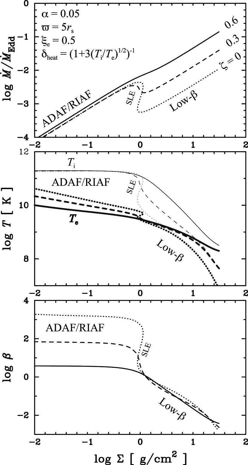
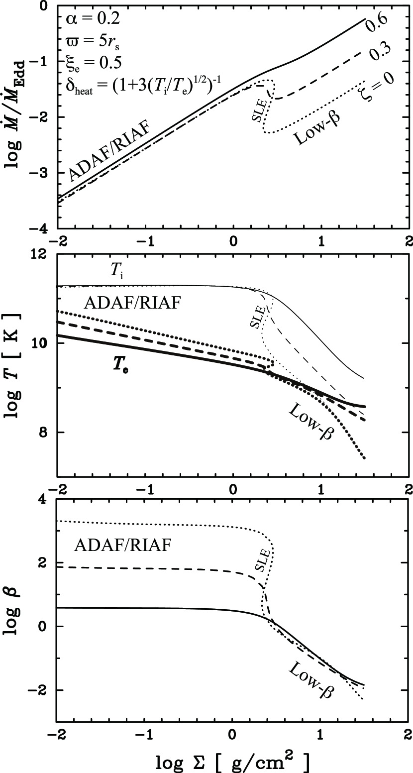
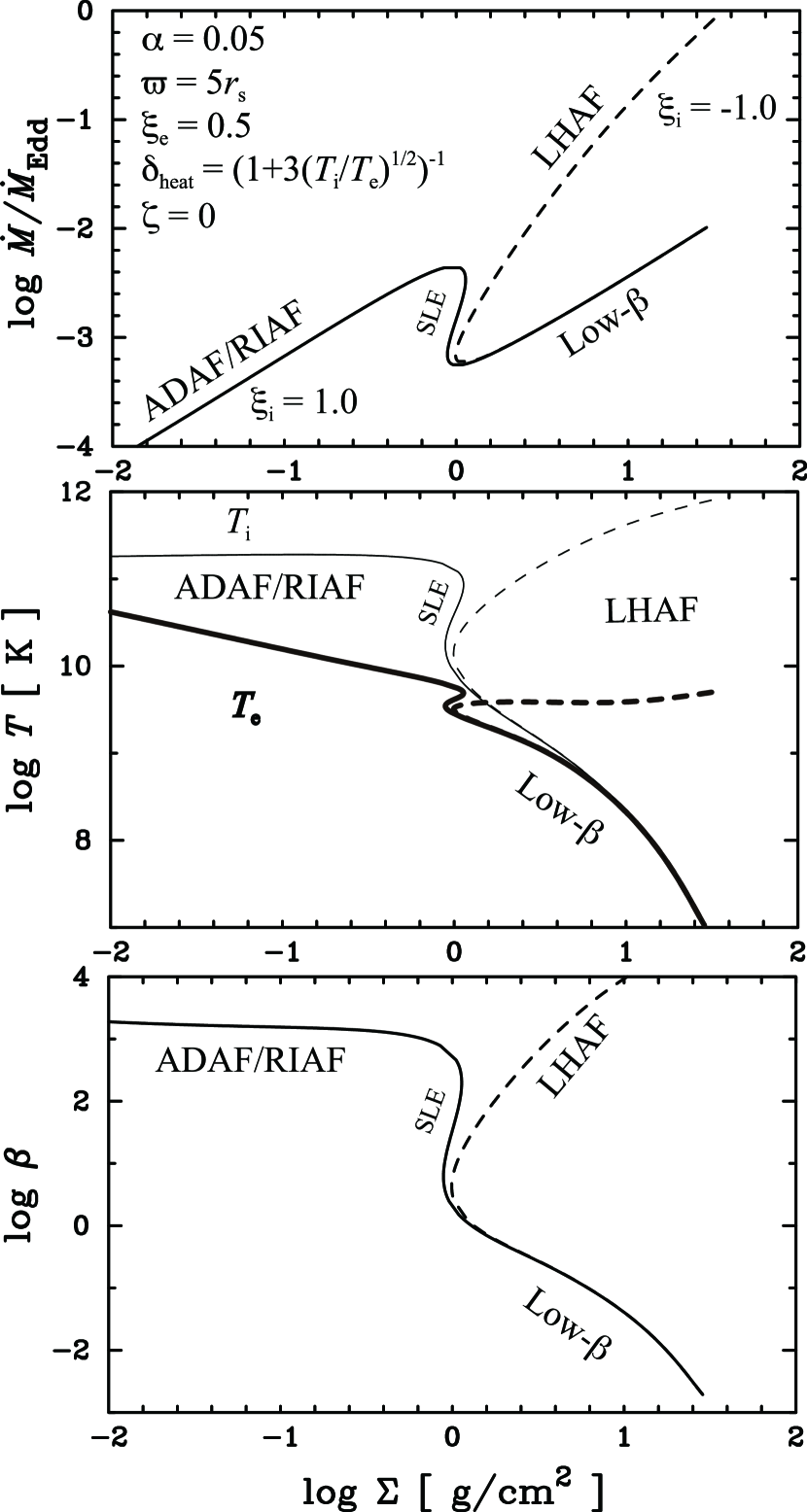
Figure 1 shows the sequences of each thermal equilibrium solution in the $\Sigma$ versus $\dot{M}/{\dot{M}}_{\rm Edd}$, $T_{\rm i}$(thin line), $T_{\rm e}$(thick line), and $\beta$ plane. The disk parameters we adopted are $\alpha=0.05$, $\xi_{\rm i}=1$, $\xi_{\rm e}=0.5$, $\delta_{\rm heat}=(1+3\sqrt{T_{\rm i}/T_{\rm e}})^{-1}$, $\zeta=0.6$ (solid), $0.3$ (dashed), and 00 (dotted), respectively. Here ${\dot{M}}_{\rm Edd}=L_{\rm Edd}/\eta_{\rm e}c^{2}=4\pi GM/\left(\eta_{\rm e}\kappa_{\rm es}c\right)$ is the Eddington mass accretion rate, $\eta_{\rm e}=0.1$ is the energy conversion efficiency, and $\kappa_{\rm es}=0.40~{}{\rm cm}^{2}~{}{\rm g}^{-1}$ is the electron scattering opacity. We obtain three types of solutions, ADAF/RIAF (for $\Sigma\lesssim 1~{}{\rm g}~{}{\rm cm}^{-2}$ at this radius), SLE (for $\Sigma\sim 1~{}{\rm g}~{}{\rm cm}^{-2}$), and low-$\beta$ solutions (for $\Sigma\gtrsim 1~{}{\rm g}~{}{\rm cm}^{-2}$). We find that the low-$\beta$ solutions exist above the maximum mass accretion rate of the ADAF/RIAF solutions, ${\dot{M}}_{\rm c,A}\sim 0.003{\dot{M}}_{\rm Edd}$. This indicates that the disk initially staying in the ADAF/RIAF state undergoes transition to the low-$\beta$ state when the mass accretion rate exceeds ${\dot{M}}_{\rm c,A}$. Furthermore, the electron temperature in the low-$\beta$ solutions is lower ($T_{\rm e}\sim 10^{8}-10^{9.5}{\rm K}$) than that in the ADAF/RIAF solutions.

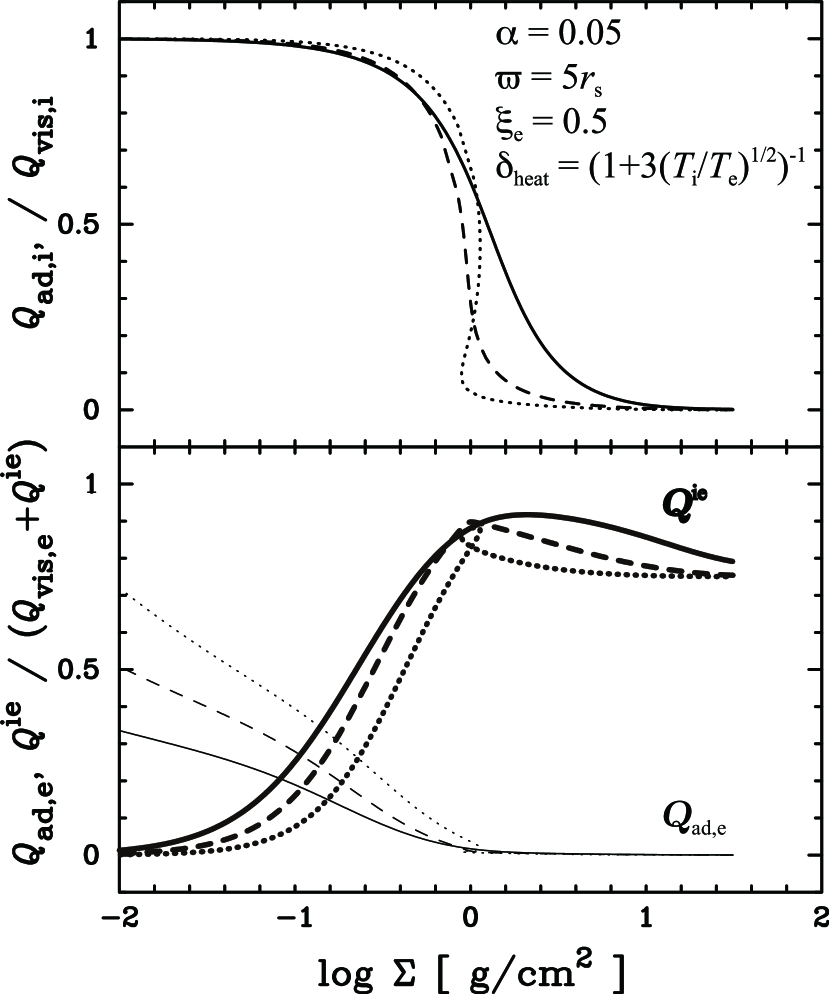
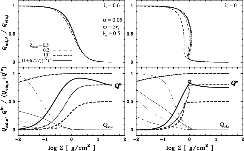
The energy balance for ions and electrons is illustrated in figure 2. The upper panel shows the ratio of the heat advection to the magnetic heating for ions, $Q_{\rm ad,i}/(1-\delta_{\rm heat})Q^{+}$ (this quantity is referred to as the advection factor $f$, e.g., Narayan & Yi, 1994, 1995; Abramowicz et al., 1995; Yuan, 2001). The lower panel shows the ratio of the heat advection to the total heating for electrons (thin line) and the fraction of the energy transfer via Coulomb collisions to the total heating (thick line). The electrons receive the total amount of the magnetic heating in the low-$\beta$ solutions as well as in the SLE solutions even though we introduced the parameter $\delta_{\rm heat}$ which represents the fraction of heating to electrons. The fraction $(1-\delta_{\rm heat})$ of the magnetic heating goes into ions and the fraction $\delta_{\rm heat}$ of the magnetic heating goes into electrons. However, almost all the magnetic heating going into ions is transferred to electrons via Coulomb collisions in the low-$\beta$ solutions ($(1-\delta_{\rm heat})Q^{+}\sim Q^{\rm ie}$). Eventually, the total amount of the magnetic heating goes into electrons. This means that the parameter $\delta_{\rm heat}$ does not appear practically in the energy balance for electrons. The radiative cooling overwhelms the heat advection in the low-$\beta$ solutions. Therefore, the magnetic heating balances the radiative cooling in the low-$\beta$ solutions ($Q^{+}\sim Q_{\rm rad}^{-}$).

The energy balance is essentially the same in both the SLE solutions and the low-$\beta$ solutions ($Q^{+}\sim Q_{\rm rad}^{-}$). The difference is which pressure dominates the magnetic heating. The magnetic heating, which is proportional to the total pressure in our model, is dominated by the gas pressure in the SLE solutions and the magnetic pressure in the low-$\beta$ solutions.

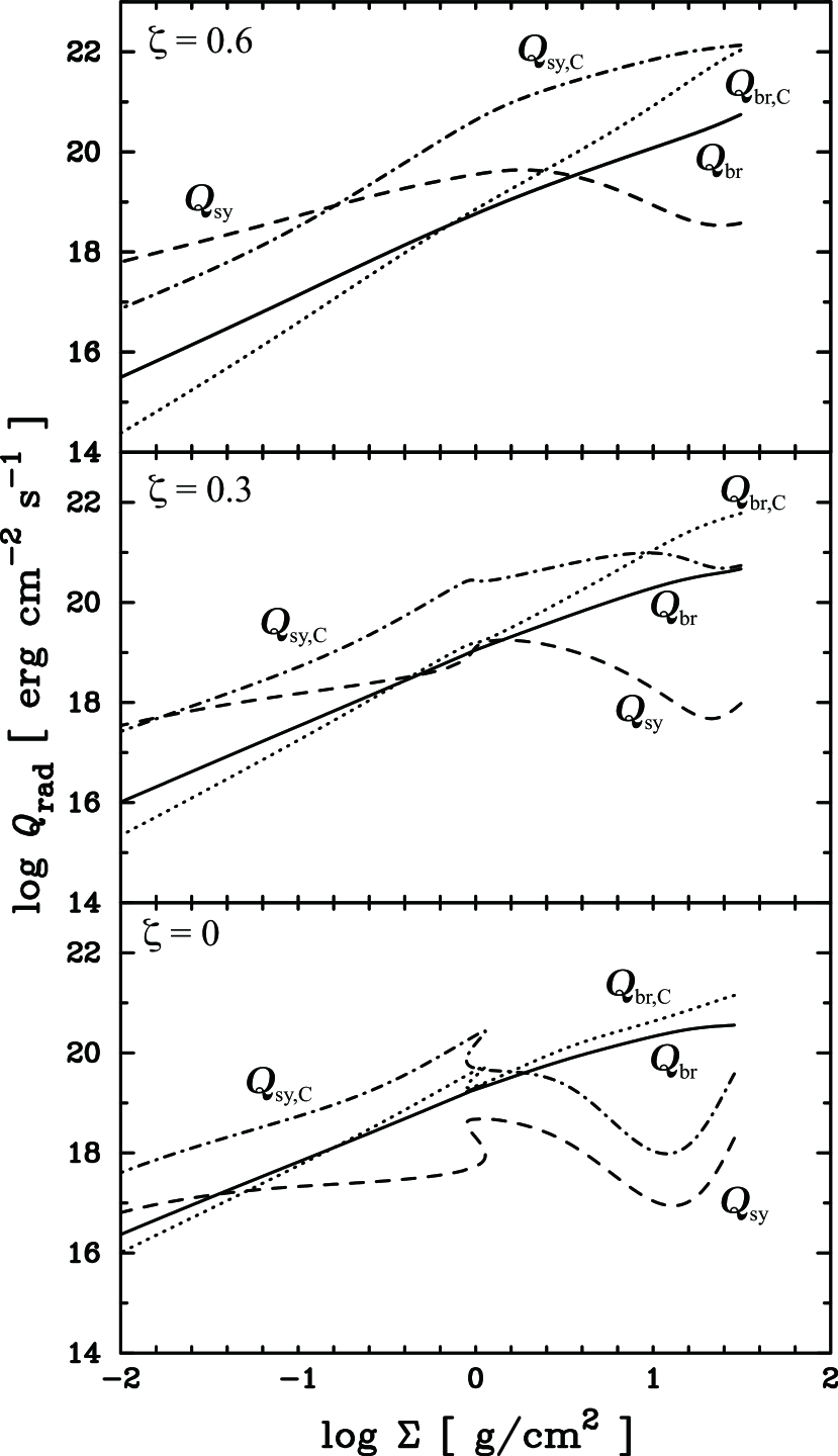
Next we describe the main cooling mechanism in each solution. Figure 3 shows the vertically integrated bremsstrahlung (solid), bremsstrahlung-Compton (dotted), synchrotron (dashed), and synchrotron-Compton (dash-dotted) cooling rate for $\zeta=0$ (bottom), $0.3$ (middle), and $0.6$ (top). When $\zeta=0$, the synchrotron-Compton cooling is dominant in the low-$\beta$ solutions for lower mass accretion rate while the bremsstrahlung-Compton cooling is dominant for high mass accretion rates ($\dot{M}\gtrsim 10^{-3}{\dot{M}}_{\rm Edd}$, $\Sigma\gtrsim 1.6~{}{\rm g}~{}{\rm cm}^{-2}$) even though $\beta<1$. The synchrotron cooling is relatively ineffective for higher mass accretion rates because of the lower electron temperature. As $\zeta$ increases, the electron temperature become high because the large magnetic flux enhances not only the synchrotron cooling but also the magnetic heating. As a result, the synchrotron and synchrotron-Compton cooling become efficient. When $\zeta=0.6$, the synchrotron-Compton is dominant in whole low-$\beta$ solutions.

Now we show that $\dot{M}\propto\Sigma$, $T\propto\Sigma^{-2}$, $\beta\propto\Sigma^{-2}$ on the low-$\beta$ branch (see also Oda et al., 2009), where $T=(T_{\rm i}+T_{\rm e})/2$ is the mean temperature. These relations depend on the dependence of ${\dot{\Phi}}_{\rm out}$ on $\dot{M}$ (our outer boundary condition leads ${\dot{\Phi}}\propto{\dot{M}}^{1/2}$). Here we introduce the parameter $s$, ${\dot{\Phi}}_{\rm out}\propto{\dot{M}}^{s}$, in order to leave this dependence explicitly. First, we derive the relations between $\dot{M}$ and $\Sigma$. Since $W_{\rm tot}\sim W_{\rm mag}\propto T\Sigma\beta^{-1}$ on the low-$\beta$ branch, equations (17), (21), and (26) yield $H\propto T^{1/2}\beta^{-1/2}$ and $\dot{M}\propto T\Sigma\beta^{-1}$. Using equations (19), (2.3), and (31), we find that $H\propto\Sigma^{-(1-2s)/(7-4s)}$, $\beta\propto\Sigma^{2(1-2s)/(7-4s)}T$, and $\dot{M}\propto\Sigma^{1-2(1-2s)/(7-4s)}$. Next, we derive the relation between $T$ and $\Sigma$ from the energy balance of the low-$\beta$ solutions ($Q^{+}\sim Q_{\rm rad}^{-}$). Here we roughly approximate the radiative cooling rate by $Q_{\rm rad}^{-}\propto\Sigma^{2}T^{1/2}H^{-1}$ for simplicity (this is the same dependence as non-relativistic bremsstrahlung cooling for single temperature plasma). Since $Q^{+}\propto W_{\rm tot}\propto\dot{M}$, we find that $T\propto\Sigma^{-2-6(1-2s)/(7-4s)}$. Therefore $\beta\propto\Sigma^{2(1-2s)/(7-4s)}T\propto\Sigma^{-2-4(1-2s)/(7-4s)}$. We find that $\dot{M}\propto\Sigma$, $T\propto\Sigma^{-2}$, and $\beta\propto\Sigma^{-2}$ when $s=1/2$.

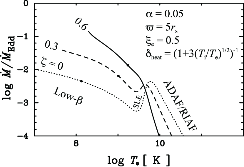
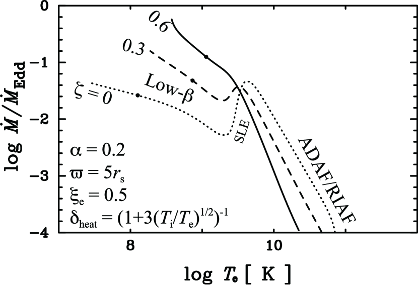
We investigate the relation between the mass accretion rate and the electron temperature in order to explain the anti-correlation between the luminosity and the cutoff energy observed in the bright/hard state. In the low-$\beta$ solutions, we expect that the luminosity is roughly proportional to the mass accretion rate since $Q_{\rm rad}^{-}\sim Q^{+}\propto\dot{M}$, and that the electron temperature roughly represents the cutoff energy since the inverse-Compton scattering is the dominant radiative cooling mechanism. Therefore, the relation between the electron temperature and the mass accretion rate is useful for comparison with the observational data. Figure 4 shows the relations between the electron temperature and the mass accretion rate for the same parameters as in Figure 1. We find that the electron temperature is typically $\lesssim 10^{9.5}~{}{\rm K}$ in the low-$\beta$ solutions while it is $\gtrsim 10^{9.5}~{}{\rm K}$ in the ADAF/RIAF solutions. Furthermore, the electron temperature in the low-$\beta$ solutions strongly anti-correlates with the mass accretion rate. Since $\dot{M}\propto\Sigma^{1-2(1-2s)/(7-4s))}$ and $T\propto\Sigma^{-2-6(1-2s)/(7-4s)}$ in the low-$\beta$ solutions, we find that $T\propto{\dot{M}}^{-2-2(1-2s)}\propto{\dot{M}}^{-2}$ for $s=1/2$.

According to Pessah & Psaltis (2005), the MRI is stabilized for $v_{\rm A}\gtrsim\sqrt{c_{\rm s}v_{\rm K0}}$ (we plot this critical point (filled circle in Figure 4) at which $v_{\rm A}=\sqrt{c_{\rm s}v_{\rm K0}}$). Therefore, the low-$\beta$ solutions may not exist under the condition that $v_{\rm A}\gtrsim\sqrt{c_{\rm s}v_{\rm K0}}$. We discuss this issue in Section 4.

We also show the results for $\alpha=0.2$ in Figure 5 and 6. The maximum mass accretion rate of the ADAF/RIAF solution is around ${\dot{M}}_{\rm c,A}\sim 0.05{\dot{M}}_{\rm Edd}$. This maximum mass accretion rate is higher than that for $\alpha=0.05$. Here we investigate the dependence of ${\dot{M}}_{\rm c,A}$ on $\alpha$. Since $W_{\rm tot}\sim W_{\rm gas}$, $Q_{\rm ad,i}/(1-\delta_{\rm heat})Q^{+}\sim 0.5$ and $Q_{\rm ad,e}\ll\delta_{\rm heat}Q^{+}+Q^{\rm ie}$ at $\dot{M}\sim{\dot{M}}_{\rm c,A}$, the energy equations yield (i) $Q_{\rm ad,i}\sim 0.5(1-\delta_{\rm heat})Q^{+}$, (ii) $Q^{\rm ie}\sim 0.5(1-\delta_{\rm heat})Q^{+}$, and (iii) $\delta_{\rm heat}Q^{+}+Q^{\rm ie}\sim[\delta_{\rm heat}+0.5(1-\delta_{\rm heat})]Q^{+}\sim Q_{\rm rad}^{-}$. Here we assume $\delta_{\rm heat}$ to be constant for simplicity. We find from Equation (i) that $T_{\rm i}\sim 10^{11}{\rm K}$. If $Q_{\rm rad}^{-}$ can be written in a simple form of $\Sigma^{2}/H\times f(T_{\rm e})$ like $Q_{\rm br}^{-}$, we find from Equations (ii) and (iii) that $T_{\rm e}$ at ${\dot{M}}_{\rm c,A}$ is independent of $\alpha$ and ${\dot{M}}_{\rm c,A}$ is proportional to $\alpha^{2}{\dot{M}}_{\rm Edd}$ exactly. Although $Q_{\rm rad}^{-}$ has a complicated form in our model, our numerical results indicate that the $T_{\rm e}$ is roughly independent of $\alpha$ ($T_{\rm e}\sim 10^{9.5}{\rm K}$). Using this value of $T_{\rm e}$ instead of solving Equation (iii), we find from Equation (ii) that roughly ${\dot{M}}_{\rm c,A}\sim\alpha^{2}{\dot{M}}_{\rm Edd}$. This result is consistent with ${\dot{M}}_{\rm c,A}\sim 1.3√\alpha^{2}{\dot{M}}_{\rm Edd}$ by Esin et al. (1997).

3.2 Effect of $\delta_{\rm heat}$

We investigated the dependence of the results on $\delta_{\rm heat}$ because $\delta_{\rm heat}$ is a poorly constrained parameter. We considered three cases: $\delta_{\rm heat}=0.5$ as an example of model in which ions and electrons receive equal amounts of the dissipated magnetic energy, $\delta_{\rm heat}=10^{-3}$ ($\sim m_{\rm e}/m_{\rm i}$) as an example of a conventional model in which ions receive a substantial amount of the energy, and $\delta_{\rm heat}=0.2$ as an intermediate example. We note that $\delta_{\rm heat}=(1+3\sqrt{T_{\rm i}/T_{\rm e}})^{-1}$ lies between $\sim 0.05$ and $0.25$ in the solutions presented in this paper.

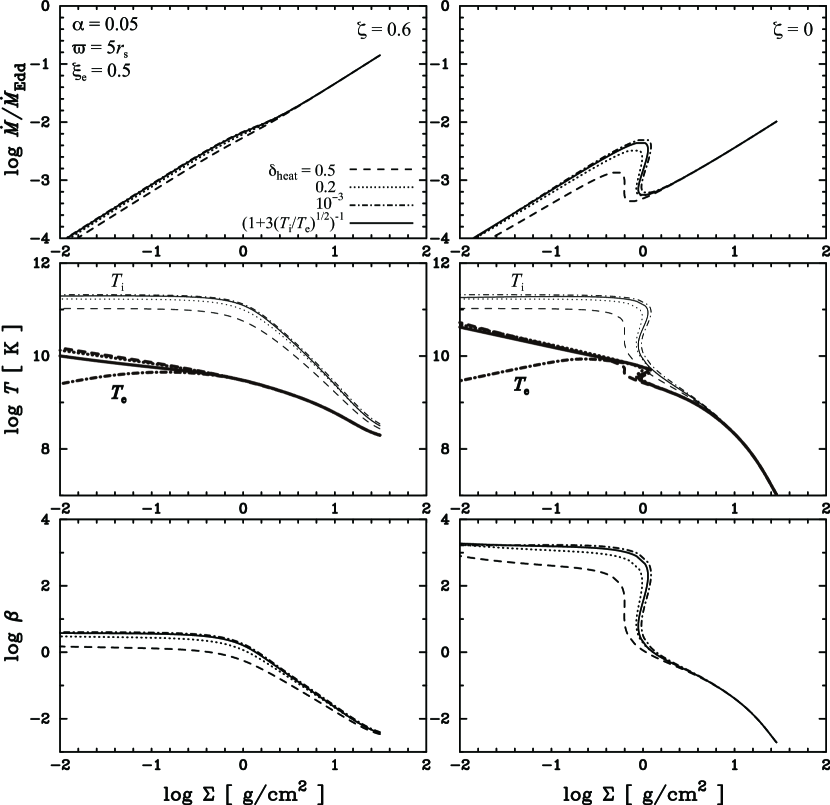
Figure 7 shows the thermal equilibrium curves for the same parameters as in Figure 1 but for $\delta_{\rm heat}=(1+3\sqrt{T_{\rm i}/T_{\rm e}})^{-1}$ (solid), $0.5$ (dashed), $0.2$ (dotted), and $10^{-3}$ (dot-dashed), respectively. The energy balance for ions and electrons is illustrated in Figure 8.

The ion temperature decreases as $\delta_{\rm heat}$ increases because the magnetic heating for ions ($(1-\delta_{\rm heat})Q^{+}$) which is the only heating source for ions decreases. ${\dot{M}}_{\rm c,A}$ also decreases because of the decrease in the magnetic heating for ions. The electron temperature increases as $\delta_{\rm heat}$ increases in the ADAF/RIAF solutions. By contrast, in the low-$\beta$ solutions, the electron temperature is almost independent of the value of $\delta_{\rm heat}$ because $\delta_{\rm heat}$ does not appear practically in the energy equation for electrons ($\delta_{\rm heat}Q^{+}+Q^{\rm ie}\sim Q^{+}\sim Q_{\rm rad}^{-}$). Therefore, we find that the exact value of $\delta_{\rm heat}$ is not so important for the low-$\beta$ solutions.

3.3 Dependence on the entropy gradient parameters, $\xi_{\rm i}$ and $\xi_{\rm e}$

Figure 9 shows the thermal equilibrium curves for the same parameters as in Figure 1 but for $\xi_{\rm i}=-1.0$ (dashed). We also plotted the thermal equilibrium curves for $\xi_{\rm i}=1.0$ (solid) for comparison.

We obtained the LHAF solutions in the high mass accretion rate and high surface density region. The heat advection works as a heating for ions and balances the energy transfer via the Coulomb collisions in the LHAF solutions. Above ${\dot{M}}_{\rm c,A}$, the heat advection term overwhelms the magnetic heating. Hence, the ion temperature becomes higher than that in the ADAF/RIAF solutions.

In the LHAF solutions, the electrons receive a larger amount of heat from ions than that in the ADAF/RIAF solutions. Nonetheless, the electron temperature becomes lower than that in the ADAF/RIAF solutions (yet higher than that in the low-$\beta$ solutions) because the radiative cooling becomes more effective in such higher surface density region.

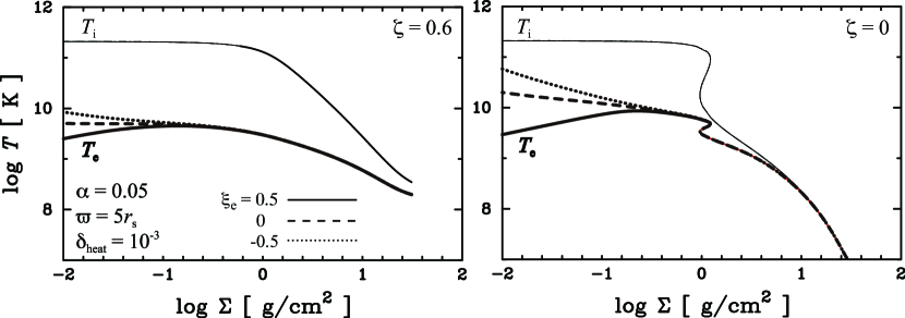
We find that our results are practically unchanged for any value of $\xi_{\rm e}$ between $-0.5$ and $0.5$ because the heat advection term is negligible compared to the other terms in energy equation for electrons except when $\delta_{\rm heat}=10^{-3}$. Furthermore, even when $\delta_{\rm heat}=10^{-3}$, the other quantities except the electron temperature in the ADAF/RIAF solutions does not change practically. We show the thermal equilibrium curves plotted on the $\Sigma$ - $T_{\rm i}$ (thin) and $T_{\rm e}$ (thick) plane for $\delta_{\rm heat}=10^{-3}$, $\xi_{\rm e}=0.5$ (solid), 00 (dashed), $-0.5$ (dotted), $\zeta=0.6$ (left panel), and 00 (right panel) in Figure 10.

4 Discussion

4.1 Optically Thin, Magnetically Supported, Moderately Cool Disks

We obtained thermal equilibrium solutions for an optically thin, two-temperature accretion disk incorporating magnetic fields. We included bremsstrahlung emission, synchrotron emission, and inverse Compton scattering as the radiative cooling mechanisms, and introduced the parameter $\delta_{\rm heat}$ which represents the fraction of the magnetic heating to electrons. We prescribed the $\varpi\varphi$-component of the azimuthally averaged Maxwell stress is proportional to the total pressure. In order to complete the set of basic equations, we specified the radial distribution of the magnetic flux advection rate by introducing a parameter $\zeta$. We found a branch of low-$\beta$ solutions in addition to the usual ADAF/RIAF (for $\xi_{\rm i}>0$), SLE, and LHAF (for $\xi_{\rm i}<0$) solutions.

Here we remark why we can obtain the low-$\beta$ solutions. First, we prescribed that the $\varpi\varphi$-component of the Maxwell stress is proportional to the total pressure. Therefore, if the magnetic pressure is high, we can obtain the magnetic heating rate balancing the radiative cooling rate even in high surface density and low temperature region. Second, we specified the magnetic flux advection rate, $\dot{\Phi}$, in order to complete the set of the basic equations. In the conventional theory, $\beta$ is assumed to be constant (typically, $\beta\sim 1$), which means that the magnetic pressure is proportional to the gas pressure. This implies that $p_{\rm gas}$ is just multiplied by a constant ($(1-\beta^{-1})p_{\rm gas}$). As a result, we cannot obtain the sequence of the low-$\beta$ solutions. On the other hand in our model, a decrease in temperature results in an increase in magnetic pressure (therefore an increase in the magnetic heating) under the conservation of the magnetic flux in the vertical direction. This is the reason why we can obtain the sequence of the low-$\beta$ solutions.

We note that the exact values of $\xi_{\rm i}$, $\xi_{\rm e}$, and $\delta_{\rm heat}$ are not so important in the low-$\beta$ solutions. The magnetic heating enhanced by the high magnetic pressure balances the radiative cooling in the low-$\beta$ solutions. The heat advection terms including $\xi_{\rm i}$ and $\xi_{\rm e}$ are negligible for both ions and electrons. Furthermore, $\delta_{\rm heat}$ does not appear in the energy balance for electrons practically.

Let us discuss the lower limit of $\beta$. Since $\beta\propto\Sigma^{-2}$ and $\Sigma\propto\dot{M}$ under our outer boundary condition ($s=1/2$), we find that $\beta\propto{\dot{M}}^{-2}$, that is, $\beta$ decreases as the mass accretion rate increases in the low-$\beta$ solutions. It has been confirmed by global MHD simulations (e.g., Machida et al., 2006) that the MRI is not stabilized and hence the magnetic heating rate is expressed in the form of equation (32), at least, when $\beta\gtrsim 0.1$. Local MHD simulations (e.g., Johansen & Levin, 2008) also indicated that the Maxwell and Reynolds stresses generated by magnetic turbulence are significant and yield an effective $\alpha$-viscosity ($\alpha\sim 0.1$) in highly magnetized disks ($\beta\sim 1$). However, the expression of the magnetic heating employed in our paper may no longer be valid for much lower values of $\beta$ because strong magnetic fields suppress the growth of the MRI. We implicitly assumed that the dissipation energy of the turbulent magnetic fields generated by the MRI is converted into the thermal energy of the disk gas. Therefore, such heating mechanism becomes ineffective if the MRI is stabilized. Pessah & Psaltis (2005) studied the evolution of the MRI in differentially rotating, magnetized flows beyond the weak-field limit, and showed that the MRI is stabilized for toroidal Alfvén speeds, $v_{\rm A}=B_{\varphi}/\sqrt{4\pi\rho_{0}}$, exceeding the geometric mean of the sound speed, $c_{\rm s}$, and the rotational speed, $v_{\rm K}=\varpi\Omega_{\rm K0}$, (i.e., $v_{\rm A}\gtrsim\sqrt{c_{\rm s}v_{\rm K0}}$, or equivalently $\beta\lesssim 2c_{\rm s}/v_{\rm K0}$). Our results satisfy this condition when $\beta\lesssim 0.27~{}(\zeta=0.6)$, $0.09~{}(\zeta=0.3)$, $0.03~{}(\zeta=0)$ for $\alpha=0.05$, and $\beta\lesssim 0.26~{}(\zeta=0.6)$, $0.08~{}(\zeta=0.3)$, and $0.02~{}(\zeta=0)$ for $\alpha=0.2$, respectively. These critical points are denoted by filled circles in Figure 4 and 6 (see also Table 1). When $\beta$ falls below this critical value, the low-$\beta$ solutions may not exist because there is no heating source balancing the radiative cooling. As a result, the disk may undergo a transition to other states (e.g, an MDAF-like disk or an optically thick disk).

4.2 Thermal Stability

Let us discuss the thermal stability in this subsection. A general criterion concerning the thermal instability of disks can be expressed as (see Pringle, 1976; Kato et al., 2008)

$\displaystyle\left[\frac{\partial}{\partial T}\left(-Q_{\rm ad}+Q^{+}-Q_{\rm rad}^{-}\right)\right]_{\Sigma}>0~{}.$ (67)

In the low-$\beta$ solutions, we ignore the heat advection term because $Q^{+}\sim Q_{\rm rad}^{-}\gg Q_{\rm ad}$. Once again we approximate the radiative cooling rate by $Q_{\rm rad}^{-}\propto\Sigma^{2}T^{1/2}H^{-1}$ for simplicity. We find from $Q^{+}\propto W_{\rm mag}\propto T\Sigma\beta^{-1}\propto\Sigma^{1-2(1-2s)/(7-4s)}$ and $Q_{\rm rad}^{-}\propto\Sigma^{2}T^{1/2}H^{-1}\propto\Sigma^{2+(1-2s)/(7-4s)}T^{1/2}$ (see Section 3.1) that the low-$\beta$ solutions do not satisfy the criterion (67), that is, are thermally stable. We note that the thermal stability is independent of $s$.

We also remark the thermal stability of the other solutions (ADAF/RIAF, SLE, and LHAF) in which the gas pressure is dominant ($W_{\rm tot}\sim W_{\rm gas}\propto\Sigma T$). Equations (17) and (19) yield $H\propto T^{1/2}$ and $\dot{M}\propto\Sigma T$. We find from $Q^{+}\propto W_{\rm gas}\propto\Sigma T$, $Q_{\rm rad}^{-}\propto\Sigma^{2}T^{1/2}H^{-1}\propto\Sigma^{2}$, $Q_{\rm ad}\propto\dot{M}T\xi\propto\Sigma T^{2}\xi$ that the ADAF/RIAF solutions ($Q^{+}\sim Q_{\rm ad}$) are thermally stable but the SLE ($Q^{+}\sim Q_{\rm rad}^{-}$) and LHAF ($Q_{\rm ad}\sim Q_{\rm rad}^{-}$) solutions are thermally unstable.

4.3 A Candidate for the Bright/Hard State

The main purpose of this paper is to explain the bright/hard state observed during the bright/slow transition in the rising phases of the transient outbursts of BHCs. In the low/hard state, the X-ray spectrum is described by a hard power law with a high energy cutoff at $\sim 200~{}{\rm keV}$. When their luminosity exceed $\sim 0.1L_{\rm Edd}$, these systems undergo a transition from the low/hard state to the bright/hard state. In the bright/hard state, the cutoff energy decreases from $\sim 200~{}{\rm keV}$ to $\sim 50~{}{\rm keV}$ as the luminosity increases from $\sim 0.1L_{\rm Edd}$ to $\sim 0.3L_{\rm Edd}$ (e.g., Miyakawa et al., 2008). Beyond the bright/hard state, these systems undergo a transition to the high/soft state going through the VH/SPL state.

The ADAF/RIAF solution explains the X-ray spectrum in the low/hard state because the electron temperature is high ($T_{\rm e}\gtrsim 10^{9.5}{\rm K}$). However, this solution does not exist at the high mass accretion rates and does not show the strong anti-correlation between the electron temperature and the mass accretion rate observed in the bright/hard state. The low-$\beta$ solution extends to such high mass accretion rates. Therefore, the disk initially staying in the ADAF/RIAF state undergoes transition to the low-$\beta$ state when the mass accretion rate exceeds ${\dot{M}}_{\rm c,A}$. On the low-$\beta$ branches, the electron temperature is low ($T_{\rm e}\sim 10^{8}-10^{9.5}{\rm K}$ $\sim 10-300~{}{\rm keV}$) and strongly anti-correlates with the mass accretion rate. These features are consistent with the anti-correlation between the luminosity and the energy cutoff observed in the bright/hard state. Therefore, the low-$\beta$ solution can explain the bright/hard state.

In Section 4.1, we have discussed the lower limit of $\beta$ below which the MRI is stabilized therefore the low-$\beta$ solutions may not exist. Since $\beta\propto{\dot{M}}^{-2}$ in the low-$\beta$ solutions, this means that the low-$\beta$ solution has a maximum mass accretion rate, ${\dot{M}}_{{\rm c,}\beta}$. The mass accretion rate and the electron temperature at the lower limit of $\beta$ are depicted by filled circles in Figure 4 and 6 (see also Table 1). We found that when $\zeta\gtrsim 0.3$ (or equivalently, $\dot{\Phi}(\varpi=5r_{\rm s})\gtrsim 4.9{\dot{\Phi}}_{\rm out}$) ${\dot{M}}_{{\rm c,}\beta}>{\dot{M}}_{\rm c,A}$. This indicates that the disk staying in the ADAF/RIAF state undergoes transition to the low-$\beta$ disk when the mass accretion rate exceeds ${\dot{M}}_{\rm c,A}$, after that, the disk undergoes transition to the optically thick disk when the mass accretion rate exceeds ${\dot{M}}_{{\rm c,}\beta}$. In this case, the hard-to-soft transition occurs at ${\dot{M}}_{{\rm c,}\beta}$ (not at ${\dot{M}}_{\rm c,A}$). This can correspond to the bright/slow transition.

Here we also remark on the dark/fast transition during which the system undergoes transition from the low/hard state to the high/soft state without going through the bright/hard state and the VH/SPL state. We found that when $\zeta\lesssim 0.3$ (or equivalently, $\dot{\Phi}(\varpi=5r_{\rm s})\lesssim 4.9{\dot{\Phi}}_{\rm out}$) ${\dot{M}}_{{\rm c,}\beta}<{\dot{M}}_{\rm c,A}$, that is, there is no optically thin, thermally stable solution above ${\dot{M}}_{\rm c,A}$. Therefore, the disk staying in the ADAF/RIAF state immediately undergoes transition to an optically thick disk without through the low-$\beta$ disk. This can correspond to the dark/fast transition. Accordingly, we conclude that the bright/slow transition occurs when $\dot{\Phi}$ has a large value and the dark/fast transition occurs when $\dot{\Phi}$ has a small value.

5 Summary

We have obtained the low-$\beta$ solutions for optically thin, two-temperature accretion disks incorporating the mean azimuthal magnetic fields, and concluded that the low-$\beta$ solutions explain the bright/hard state observed during the bright/slow transition of BHCs. We assumed that the energy transfer from ions to electrons occurs through Coulomb collisions, and considered bremsstrahlung emission, synchrotron emission, and inverse Compton scattering as the radiative cooling processes. We prescribed that the Maxwell stress is proportional to the total (gas and magnetic) pressure. In order to complete the set of basic equations, we specified the radial distribution of the magnetic flux advection rate. Accordingly, a decrease in temperature can result in an increase in magnetic pressure under the conservation of the magnetic flux in the vertical direction. In the low-$\beta$ solutions, the magnetic heating is enhanced by the high magnetic pressure. The fraction $(1-\delta_{\rm heat})$ of the magnetic heating goes into ions and is transferred to electrons via Coulomb collisions. The fraction $\delta_{\rm heat}$ of the magnetic heating goes into electrons. Eventually, the total amount of the magnetic heating goes into electrons and balances the radiative cooling (Compton cooling by bremsstrahlung and/or synchrotron photons). The electron temperature is lower than that in the ADAF/RIAF solutions ($T_{\rm e}\sim 10^{8}-10^{9.5}{\rm K}\sim 10-300~{}{\rm keV}$) and strongly anti-correlates with the mass accretion rate in the low-$\beta$ solutions. These features are consistent with the X-ray spectrum observed in the bright/hard state.

According to Pessah & Psaltis (2005), the MRI is stabilized for $\beta\lesssim 2c_{\rm s}/v_{\rm K0}$. This indicates that the low-$\beta$ solutions disappear below this critical point. When the magnetic flux advection rate is high ($\zeta\gtrsim 0.3$), the critical mass accretion rate of the low-$\beta$ solutions, ${\dot{M}}_{{\rm c,}\beta}$, is above the maximum mass accretion rate of the ADAF/RIAF solutions, ${\dot{M}}_{\rm c,A}$. Therefore, the disk initially staying the ADAF/RIAF state undergoes transition to the low-$\beta$ state when the mass accretion rate exceeds ${\dot{M}}_{\rm c,A}$, after that, the disk undergoes transition to the optically thick disk when the mass accretion rate exceeds ${\dot{M}}_{{\rm c,}\beta}$. This corresponds to the bright/slow transition. On the other hand, when the magnetic flux advection rate is low ($\zeta\lesssim 0.3$), ${\dot{M}}_{{\rm c,}\beta}$ is below ${\dot{M}}_{\rm c,A}$. Therefore, the disk initially staying the ADAF/RIAF state immediately undergoes transition to the optically thick disk when the mass accretion rate exceeds ${\dot{M}}_{\rm c,A}$. This can correspond to the dark/fast transition.

We are grateful to R. Narayan for valuable discussion and closely examining my draft. This work is supported by the Grant-in-Aid for Science Research of the Ministry of Education, Culture, Sports, Science and Technology (RM: 20340040) and Grant-in-Aid for JSPS Fellows (20.1842).

References

  • Abramowicz et al. (1995) Abramowicz, M. A., Chen, X., Kato, S., Lasota, J.-P., & Regev, O. 1995, ApJ, 438, L37
  • Balbus & Hawley (1991) Balbus, S. A., & Hawley, J. F. 1991, ApJ, 376, 214
  • Belloni et al. (2006) Belloni, T., et al. 2006, MNRAS, 367, 1113
  • Dermer et al. (1991) Dermer, C. D., Liang, E. P., & Canfield, E. 1991, ApJ, 369, 410
  • Eardley et al. (1975) Eardley, D. M., Lightman, A. P., & Shapiro, S. L. 1975, ApJ, 199, L153
  • Esin et al. (1997) Esin, A. A., McClintock, J. E., & Narayan, R. 1997, ApJ, 489, 865
  • Esin et al. (1998) Esin, A. A., Narayan, R., Cui, W., Grove, J. E., & Zhang, S.-N. 1998, ApJ, 505, 854
  • Esin et al. (1996) Esin, A. A, Narayan, R., Ostriker, E., & Yi, I. 1996, ApJ, 465, 312
  • Fragile & Meier (2009) Fragile, P. C., & Meier, D. L. 2009, ApJ, 693, 771
  • Gierliński & Newton (2006) Gierliński, M., & Newton, J. 2006, MNRAS, 370, 837
  • Hawley (2000) Hawley, J. F. 2000, ApJ, 528, 462
  • Hawley & Krolik (2001) Hawley, J. F. & Krolik, J. H. 2001, ApJ, 548, 348
  • Hirose et al. (2006) Hirose, S., Krolik, J. H., & Stone, J. M. 2006, ApJ, 640, 901
  • Ichimaru (1977) Ichimaru, S. 1977, ApJ, 214, 840
  • Johansen & Levin (2008) Johansen, A., & Levin, Y. 2008, A&A, 490, 501
  • Kato et al. (2008) Kato, S., Fukue, J., & Mineshige, S. 2008, Black-Hole Accretion Disks: Towards a New Paradigm (Kyoto: Kyoto Univ. Press)
  • Krolik et al. (2007) Krolik, J. H., Hirose, S., & Blaes, O. 2007, ApJ, 664, 1045
  • Machida et al. (2000) Machida, M., Hayashi, M. R., & Matsumoto, R. 2000, ApJ, 532, L67
  • Machida & Matsumoto (2003) Machida, M., & Matsumoto, R. 2003, ApJ, 585, 429
  • Machida et al. (2004) Machida, M., Nakamura, K. E., & Matsumoto, R. 2004, PASJ, 56, 671
  • Machida et al. (2006) Machida, M., Nakamura, K. E., & Matsumoto, R. 2006, PASJ, 58, 193
  • Mahadevan et al. (1996) Mahadevan, R., Narayan, R., & Yi, I. 1996, ApJ, 456, 327
  • Manmoto et al. (1997) Manmoto, T., Mineshige, S., & Kusunose, M. 1997, ApJ, 489, 791
  • Meier (2005) Meier, D. L. 2005, Ap&SS, 300, 55
  • Miyakawa et al. (2008) Miyakawa, T., Yamaoka, K., Homan, J., Saito, K., Dotani, T., Yoshida, A., & Inoue, H. 2008, PASJ, 60, 637
  • Nakamura et al. (1997) Nakamura, K. E., Kusunose, M., Matsumoto, R., & Kato, S. 1997, PASJ, 49, 503
  • Nakamura et al. (1996) Nakamura, K. E., Matsumoto, R., Kusunose, M., & Kato, S. 1996, PASJ, 48, 761
  • Narayan & Yi (1994) Narayan, R., & Yi, I. 1994, ApJ, 428, L13
  • Narayan & Yi (1995) Narayan, R. & Yi, I. 1995, ApJ, 452, 710
  • Nishikori et al. (2006) Nishikori, H, Machida, M, & Matsumoto, R ApJ, 2006, 641, 862
  • Oda et al. (2007) Oda, H., Machida, M., Nakamura, K. E., & Matsumoto, R. 2007, PASJ, 59, 457
  • Oda et al. (2009) Oda, H., Machida, M., Nakamura, K. E. & Matsumoto, R. 2009, ApJ, 697, 16
  • Pacholczyk (1970) Pacholczyk, A. G. 1970, Radio Astrophysics (San Francisco, CA: Freeman)
  • Paczyńsky & Wiita (1980) Paczyńsky, B. & Wiita, P. J. 1980, A&A, 88, 23
  • Parker (1966) Parker, E. N. 1966, ApJ, 145, 811
  • Pessah & Psaltis (2005) Pessah, M. E., & Psaltis, D. 2005, ApJ, 628, 879
  • Pringle (1976) Pringle, J. E. 1976, MNRAS, 177, 65
  • Shakura & Sunyaev (1973) Shakura, N. I., & Sunyaev, R. A. 1973, A&A, 24, 337
  • Shapiro et al. (1976) Shapiro, S. L., Lightman, A. P., & Eardley, D. M. 1976, ApJ, 204, 187
  • Sharma et al. (2007) Sharma, P., Quataert, E., Hammett, G. W., & Stone, J. M. 2007, ApJ, 667, 714
  • Shibata et al. (1990) Shibata, K., Tajima, T., & Matsumoto, R. 1990, ApJ, 350, 295
  • Shibazaki & Hōshi (1975) Shibazaki, N., & Hōshi, R. 1975, Prog. Theor. Phys., 54, 706
  • Stepney & Guilbert (1983) Stepney, S., & Guilbert, P. W. 1983, MNRAS, 204, 1269
  • Svensson (1982) Svensson, R. 1982, ApJ, 258, 335
  • Thorne & Price (1975) Thorne, K. S., & Price, R. H. 1975, ApJ, 195, L101
  • Yuan (2001) Yuan, F. 2001, MNRAS, 324, 119
  • Yuan (2003) Yuan, F. 2003, ApJ, 594, L99
  • Yuan et al. (2003) Yuan, F., Quataert, E., & Narayan, R. 2003, ApJ, 598, 301
Refer to caption
Figure 1: Local thermal equilibrium curves of optically thin, two-temperature accretion disks at $\varpi=5r_{\rm s}$ in the $\Sigma$ vs. $\dot{M}/{\dot{M}}_{\rm Edd}$, $T_{\rm i}$(thin line), $T_{\rm e}$(thick line), and $\beta$ plane. The disk parameters are $\alpha=0.05$, $\xi_{\rm i}=1$, $\xi_{\rm e}=0.5$, $\delta_{\rm heat}=(1+3\sqrt{T_{\rm i}/T_{\rm e}})^{-1}$, $\zeta=0.6$ (solid), $0.3$ (dashed), and 00 (dotted). ${\dot{M}}_{\rm Edd}=L_{\rm Edd}/\eta_{\rm e}c^{2}=4\pi GM/\left(\eta_{\rm e}\kappa_{\rm es}c\right)$ is the Eddington mass accretion rate and $\eta_{\rm e}=0.1$ is the energy conversion efficiency. The equilibrium curves consist of the ADAF/RIAF, SLE, and low-$\beta$ branches.
Refer to caption
Figure 2: Energy balance for ions and electrons for the same parameters as Figure 1 (solid: $\zeta=0.6$, dashed: $\zeta=0.3$, dotted: $\zeta=0$). Upper: the ratio of the heat advection to the magnetic heating for ions, $Q_{\rm ad,i}/(1-\delta_{\rm heat})Q^{+}$ (this parameter is referred to as the advection factor $f$, e.g., Narayan & Yi, 1994, 1995; Abramowicz et al., 1995; Yuan, 2001). Lower: the ratio of the heat advection to the total heating (thin), $Q_{\rm ad,e}/(\delta_{\rm heat}Q^{+}+Q^{\rm ie})$, and the fraction of the energy transfer via Coulomb collisions to the total heating (thick), $Q^{\rm ie}/(\delta_{\rm heat}Q^{+}+Q^{\rm ie})$, for electrons.
Refer to caption
Figure 3: Vertically integrated radiative cooling rates for $\zeta=0$ (bottom), $0.3$ (middle), and $0.6$ (top). Solid: bremsstrahlung ($Q_{\rm br}$), dotted: bremsstrahlung-Compton ($Q_{\rm br,C}$), dashed: synchrotron ($Q_{\rm sy}$), and dash-dotted: synchrotron-Compton ($Q_{\rm sy,C}$).
Refer to caption
Figure 4: Relations between the electron temperature and the mass accretion rate for the same parameter as Figure 1. Filled circles represent critical points at which $v_{\rm A}=\sqrt{c_{\rm s}v_{\rm K0}}$ (or equivalently $\beta=2c_{\rm s}/v_{\rm K0}$), where $v_{\rm A}=B_{\varphi}/\sqrt{4\pi\rho_{0}}$ is the toroidal Alfvén speed, $c_{\rm s}$ is the sound speed, and $v_{\rm K}=\varpi\Omega_{\rm K0}$ is the rotational speed.
Refer to caption
Figure 5: Same as Figure 1 but for $\alpha=0.2$.
Refer to caption
Figure 6: Same as Figure 4 but for $\alpha=0.2$.
Refer to caption
Figure 7: Dependence of local thermal equilibrium curves on $\delta_{\rm heat}$. The disk parameters are $\alpha=0.05$, $\xi_{\rm i}=0.5$, $\xi_{\rm e}=0.5$, $\delta_{\rm heat}=(1+3\sqrt{T_{\rm i}/T_{\rm e}})^{-1}$ (solid), $0.5$ (dashed), $0.2$ (dotted), $10^{-3}$ (dot-dashed), $\zeta=0.6$ (left) and 00 (right). The exact value of $\delta_{\rm heat}$ is not so important for the low-$\beta$ solutions.
Refer to caption
Figure 8: Energy balance for ions and electrons for the same parameters as Figure 7 (left: $\zeta=0.6$, right: $\zeta=0$). Upper: the ratio of the heat advection to the magnetic heating for ions, $Q_{\rm ad,i}/(1-\delta_{\rm heat})Q^{+}$. Lower: the ratio of the heat advection to the total heating (thin), $Q_{\rm ad,e}/(\delta_{\rm heat}Q^{+}+Q^{\rm ie})$, and the fraction of the energy transfer via Coulomb collisions to the total heating (thick), $Q^{\rm ie}/(\delta_{\rm heat}Q^{+}+Q^{\rm ie})$, for electrons.
Refer to caption
Figure 9: Local thermal equilibrium curves for the same parameters as in Figure 1 but for $\xi_{\rm i}=-1.0$ (dashed). The equilibrium curves consist of the LHAF, SLE, and low-$\beta$ branches. We also plotted the thermal equilibrium curves for $\xi_{\rm i}=1.0$ (solid) for comparison.
Refer to caption
Figure 10: Local thermal equilibrium curves plotted on the $\Sigma$ - $T_{\rm i}$ (thin) and $T_{\rm e}$ (thick) plane for $\delta_{\rm heat}=10^{-3}$, $\xi_{\rm e}=0.5$ (solid), 00 (dashed), $-0.5$ (dotted), $\zeta=0.6$ (left panel), and 00 (right panel)
Table 1: Values at the lower limit of $\beta$
$\alpha$ $\zeta$ $\beta$ ${\dot{M}}_{{\rm c,}\beta}/{\dot{M}}_{\rm Edd}$ $T_{\rm e}~{}{\rm[K]}$
$0.05$ $0.6$ $0.27$ $1.3\times 10^{-2}$ $1.7\times 10^{9}$
$0.3$ $0.09$ $6.4\times 10^{-3}$ $1.0\times 10^{9}$
00 $0.03$ $4.5\times 10^{-3}$ $1.3\times 10^{8}$
$0.2$ $0.6$ $0.26$ $1.2\times 10^{-1}$ $1.1\times 10^{9}$
$0.3$ $0.08$ $4.8\times 10^{-2}$ $7.4\times 10^{8}$
00 $0.02$ $2.6\times 10^{-2}$ $1.3\times 10^{8}$