A Nonperturbaive Proposal for Nonabelian Tensor Gauge Theory

and

Dynamical Quantum Yang-Baxter Maps

Soo-Jong Rey ^a,b   and    Fumihiko Sugino ^c

^a School of Physics & Astronomy, Seoul National University, Seoul 151-747 KOREA

^b School of Natural Sciences, Institute for Advanced Study, Princeton NJ 08540 USA

^b Okayama Institute for Quantum Physics, Kyoyama 1-9-1, Kita-ku, Okayama 700-0015 JAPAN

sjrey@snu.ac.kr     fumihiko-sugino@pref.okayama.lg.jp

ABSTRACT

We propose a nonperturbative approach to nonabelian two-form gauge theory. We formulate the theory on a lattice in terms of plaquette as fundamental dynamical variable, and assign U($N$) Chan-Paton colors at each boundary link. We show that, on hypercubic lattices, such colored plaquette variables constitute Yang-Baxter maps, where holonomy is characterized by certain dynamical deformation of quantum Yang-Baxter equations. Consistent dimensional reduction to Wilson’s lattice gauge theory singles out unique compactness condition. We study a class of theories where the compactness condition is solved by Lax pair ansatz. We find that, in naive classical continuum limit, these theories recover Lorentz invariance but have degrees of freedom that scales as $N^{2}$ at large $N$. This implies that nontrivial quantum continuum limit must be sought for. We demonstrate that, after dimensional reduction, these theories are reduced to Wilson’s lattice gauge theory. We also show that Wilson surfaces are well-defined physical observables without ordering ambiguity. Utilizing lattice strong coupling expansion, we compute partition function and correlation functions of the Wilson surfaces. We discover that, at large $N$ limit, the character expansion coefficients exhibit large-order behavior growing faster than exponential, in striking contrast to Wilson’s lattice gauge theory. This hints a hidden, weakly coupled theory dual to the proposed tensor gauge theory. We finally discuss relevance of our study to topological quantum order in strongly correlated systems.

1 Pictures and Discussions

”What is the use” thought Alice ”of a book if it has

no picture or conversation?” — Louis Carroll

An outstanding problem in theoretical physics is a constructive definition of $p$-form gauge theories, especially, nonabelian and self-interacting ones. Variants of $p$-form gauge theory arise in diverse contexts, ranging from string or M theories [1, 2] and higher-dimensional integrable systems [3] to topological order and phases in strongly correlated systems [4] and to quantum error correction codes [5] in quantum information sciences. Of particular interest is whether a nonabelian $p$-form gauge theory exists and, if so, what sort of self-interactions are allowed by the gauge invariance. To the problem posed, one’s first guess is that the fundamental degrees of freedom are some sort of nonabelian extension of the abelian $p$-form gauge theory, but then the question is now more to ”what types of nonabelian extensions can be endowed to abelian $p$-form gauge theory?” and to ”what types of self-interaction are possible for a given nonabelian extension?”.

The ${\mathbb{Z}}_{2}$ Ising model provides the simplest situation of all. Consider the model defined on a $d$-dimensional hypercubic lattice. In dual formulation, the Ising model is mapped to a gauge theory, where the gauge potential is a $p=(d-2)$-form and takes a value in $G={\mathbb{Z}}_{2}$. As is firmly established, the Ising model does not exhibits any nontrivial renormalization group fixed point for $d\geq 4$. It implies that the dual $p$-form gauge theory in $d\geq 4$ ought to be free in the continuum limit, yielding no obvious self-interaction among the $p$-form gauge potentials .

In string and M theories, variety of the $p$-form gauge potentials is rich and complex. Foremost, all known string theories, whether supersymmetric or not, contain universally the Kalb-Ramond two-form potential $B_{2}={1\over 2!}B_{mn}{\rm d}x^{m}\wedge{\rm d}x^{n}$, and the fundamental string couples minimally to it [1]. Type I and II superstring theories contain in addition R-R(Ramond-Ramond) $p$-form potentials [2]. The D$(p-1)$-branes are the charged objects coupled minimally to these R-R potentials. Because of different chirality projection, type IIA superstring gives rise to $p=1,3,\cdots,9$ only, while Type IIB superstring does so for $p=0,2,\cdots,10$ only. These NS-NS and R-R fields exhaust all possible $p$-form potentials permeating through the ten-dimensional bulk spacetime. To the extent understood so far, they are essentially abelian.

There are, in addition, $p$-form potentials residing only on the worldvolume of string solitons. Consider first the D-branes, the objects minimally coupled to the R-R gauge potentials. At low-energy below the string scale, D-brane worldvolume dynamics is dominated by the lowest excitation of open strings whose both ends are attached to the D-brane. The excitation constitutes one-form ($p=1$) potential $A_{m}(x){\rm d}x$ of gauge group U(1) and free scalar fields. A novelty is that, when $N$ parallel D-branes stack on top of one another, combinatorially, there are $N\times N$ possible open strings and the lowest excitation of them forms U($N$) matrix-valued 1-form potential [8]. Thus, for D-branes, $N^{2}$ variety of open strings constitutes the microscopic field and particle degrees of freedom of the D-brane worldvolume. Consider next the NS5-brane, the magnetic dual to the fundamental string. Worldvolume dynamics of an NS5-brane in Type IIA string theory, equivalently, an M5-brane in M-theory is described at low-energy by the six-dimensional ${\cal N}=(2,0)$ superconformal theory [18], and the theory is known to contain a selfdual two-form ($p=2$) potential of gauge group U(1). Again, a novelty is that, when $N$ parallel NS5-branes or M5-branes stack on top of one another, the microscopic degrees of freedom constitute tensionless strings that arise in M-theory from the variety of open M2-branes connecting all possible combinatoric pairs of the $N$ M5-branes [10]. Similar to the D-branes, one might anticipate that $N^{2}$ variety of open M2-branes connecting all possible pairs of M5-brane constitute the microscopic field and string degrees of freedom of the M5-brane worldvolume. However, in stark contrast, various considerations ranging thermodynamic free energy [11] and gravitational anomaly cancellation [12] all indicate a peculiarity that the degrees of freedom are intrinsically quantum-mechanical and scales in $N\rightarrow\infty$ limit as $N^{3}$, in stark contrast to $N^{2}$ behavior [13] observed for the D3-brane worldvolume dynamics described by the ${\cal N}=4$ super Yang-Mills theory.

In this paper, we study a viable extension of nonabelian gauge invariance to tensor gauge field and put forward a nonperturbative approach for tensor gauge theory in $d\geq 4$ dimensions  by putting the theory on a $d$-dimensional hypercubic lattice. The lattice formulation allows a tranparent and concerete description for origin of nonabelian gauge symmetries and self-interactions among the $p$-form gauge fields . By putting the theory on a lattice, we are sidestepping from other structures that can be endowed to the tensor gauge theory such as (extended) supersymmetry or (anti)self-duality. Though these structures are desirable for making contact with those arising in string theory, in this paper, we focus primarily on the issue of nonabelian gauge symmetry and self-interactions thereof.

This paper is organized as follows. We begin in section 2 with etiology of Chan-Paton factors. We assign Chan-Paton factors to boundary links of an elementary plaquette so that it carries four ‘color’ indices. We take these objects as fundamental dynamical variables and construct in section 3 a nonabelian two-form tensor gauge theory defined on a $d$-dimensional hypercubic lattice. Expressing the plaquette variable as $(N^{2}\times N^{2})$ matrices of U($N$) gauge group, we construct action for nonabelian tensor gauge theory. We then study possible compactness conditions. We show that consistent reduction to Wilson’s lattice gauge theory [16] by a dimensional reduction and unitarity or reflection-positivity singles out a unique choice of the condition. In section 4, we study ground state of the lattice theory. We show that ground-state configurations are provided by vanishing holonomy of the nonabelian tensor fields. Remarkably, these configurations are specified by the solution of so-called dynamical quantum Yang-Baxter equations, pointing to an extremely rich structure of the ground-state wave function. Nontrivial holonomies are measured by a set of possible deformations of the dynamical quantum Yang-Baxter equations and their solutions. In section 6, we study Lax pair ansatz for solving the compactness condition by parametrizing the plaquette variables in terms of direct product of $(N\times N)$ matrices of U($N$) group. We then study continuum limit of the classical action, viz. naive continuum limit and point out that the gauge symmetry becomes abelian in this limit. In section 6, we show that the theory passes up an important consistency condition: upon lattice dimensional reduction, the theory is reduced to the Yang-Mills theory in the classical continuum limit. In section 7, utilizing the lattice strong-coupling expansion, we compute free energy and Wilson surface correlators. We find that in stark contrast to Polyakov-Wilson lattice gauge theory, the expansion series is not Borel summable even in the large $N$ limit. We present an intuitive argument for the behavior and argue that the large-order behavior point to the existence of a weakly interacting, dual lattice theory. Section 8 is devoted to a summary of this paper and discussion on remaining issues. In Appendix A, we explain that a truncation of the internal degrees of freedom following the dimensional reduction leads the Wilson’s lattice gauge theory at the lattice level the plaquette variables to the Wilson’s link variables. Consistency with this procedure reduces the original four possibilities of the theory into two. In Appendix B, we analyze the rank-$N$ theory and see that it does not lead a physically meaningful continuum theory under the dimensional reduction. In Appendix C, we explain solutions of the compactness condition of the rank-$N^{2}$(I) which are not expressed as a direct-product structure. Although the solutions have the ${\cal O}(N^{3})$ degrees of freedom, the gauge degrees of freedom reduce to $\left({\rm U}(1)\right)^{N}$, which does not lead to an interesting nonabelian tensor theory. Also, since the gauge degrees of freedom are not enough to eliminate modes of wrong-sign kinetic terms (ghosts), the solutions do not seem to lead physically meaningful continuum theory at least in the classical level. In Appendix D, we present some computation on a character expansion coefficient used in strong coupling expansion.

2 Etiology of Chan-Paton Factors

We begin with etiology of the Chan-Paton factors [17]. Originally, the Chan-Paton factors were introduced as a prescription for introducing “colors” to open string amplitudes. In this section, we will adapt the notion on a lattice and interpret it as endowing a Chan-Paton bundle over a finite-dimensional vector space $V_{\rm CP}$ to parallel transport.

2.1 elementary link variables

Consider the Wegner-Wilson-Polyakov formulation of the lattice gauge theory [16] on a $d$-dimensional hypercubic lattice. Taking gauge group $G$ to be compact $U(1)$, elementary degrees of freedom are associated with link variables, $U(x,x+\hat{\mu})$. This is a dynamical variable residing at each unit link (of length $a$) $[x;\hat{\mu}]$ of direction $\hat{\mu}$, connecting the nearest neighbor sites $x$ and $x+\hat{\mu}$. The link variable assigns a dynamical weight to parallel-transporting a charged particle (charge $+1$) long the unit link $[x;\hat{\mu}]$. The link variable $U_{\mu}(x)$ is parametrizable in terms of gauge potential $A_{\mu}(x)$ that takes values on $\mathbb{S}^{1}$:

$$U_{\mu}(x)\equiv U(x,x+\hat{\mu})=\exp(iaA_{\mu}(x)),$$ (2.1)

By the exponential map defined so, the link variable satisfies the compactness condition:

$$U^{-1}(x,x+\hat{\mu})=U(x+\hat{\mu},x).$$ (2.2)

As the charged particle is parallel-transported, $U_{\mu}(x)$ creates the electric charge $-1$ at the site $x$ (where a unit charge is depleted) and $+1$ at the site $x+\hat{\mu}$ (where a unit charge is deposited). For an arbitrary path on the lattice, the corresponding parallel-transport is determined by multiplying link variables along the path. Therefore, the set of all possible link variables $\{U_{\mu}(x)\}$ constitutes microscopic degrees of freedom on the lattice. Of particular interest is the parallel-transport around a unit plaquette $[x;\hat{\mu},\hat{\nu}]$:

$$U_{\rm P}\equiv U(x,x+\hat{\mu})U(x+\hat{\mu},x+\hat{\mu}+\hat{\nu})U(x+\hat{\mu}+\hat{\nu},x+\hat{\nu})U(x+\hat{\nu},x).$$

This is a gauge-invariant operator, and deviation of it from unity measures the holonomy around the unit plaquette $[x;\hat{\mu},\hat{\nu}]$.

The construction is readily extendible by adjoining Chan-Paton factors. We promote the link variable to a matrix-valued one. It comes through a pair of the Chan-Paton factors $i,j\in V_{\rm CP}$ attached at the two ends of each unit link at $x$:

$$U_{\mu}(x)\otimes|\,ij\rangle\equiv\Big{(}U_{\mu}(x)\Big{)}_{ij}$$ (2.3)

The $i,j=1,\cdots,N$ indices label an orthogonal basis of the vector space $V_{\rm CP}$, so equivalence relations and hence the gauge group $G$ would be associated with the rational map

$$G:V_{\rm CP}\rightarrow V_{\rm CP}.$$

As such, the elementary link variables are matrix-valued in GL($N,\mathbb{C}$). See Fig.1.

The Chan-Paton etiology can be restated as follows. The sites and links are 0- and 1-simplices of the $d$-dimensional hypercubic lattice. The two sites at the end of a link variable are boundary 0-simplices of a 1-simplex. To define nonabelian lattice gauge theory, we are then assigning the Chan-Paton factors $i,j,\cdots\in V_{\rm CP}$ at each boundary 0-simplex of 1-simplices. The matrix-valued holonomy is measured around the boundary of each plaquette. For the unit plaquette located at $x$ and oriented along $[\hat{\mu}\hat{\nu}]$-directions, the holonomy is measured by

$$\Big{(}U_{\mu}(x)\Big{)}_{ij}\Big{(}U_{\nu}(x+\hat{\mu})\Big{)}_{j\,k}\Big{(}U_{-\mu}(x+\hat{\mu}+\hat{\nu})\Big{)}_{k\ell}\Big{(}U_{-\nu}(x+\hat{\nu})\Big{)}_{\ell m}.$$

It measures the gauge flux felt by a colored particle around the closed loop of 1-simplices, transmuting the color through $i\rightarrow j\rightarrow k\rightarrow\ell\rightarrow m$. In the context of open strings ending on D-branes, the colored particle is nothing but an endpoint of the open string.

Figure 1: The link corresponding to the variable $(U_{\mu}(x))_{ij}$. The Chan-Paton indices $i,j$ are assigned as quantum numbers labelling the 0-simplices at the two ends of the 1-simplex defining the link variable.

The elementary link variable $(U_{\mu}(x))_{ij}$ evolves dynamically and sweeps out a plaquette $P$ (of area $a^{2}$) inside the $d$-dimensional hypercubic lattice. The Chan-Paton factor should be consistent with various closure relations. First, a product of two link variables should be isomorphic to another link variable:

$$\sum_{j=1}^{N}\Big{(}U_{\mu}(x)\Big{)}_{ij}\cdot\Big{(}U_{\mu}(x+\widehat{\mu})\Big{)}_{jk}:=\Big{(}U_{\mu}(x)U_{\mu}(x+\widehat{\mu})\Big{)}_{ik}.$$ (2.4)

Second, generalizing Eq.(LABEL:abelianunitarity), unitarity of the link variable forces the compactness condition:

$$\sum_{j=1}^{N}\Big{(}U_{\mu}(x)\Big{)}_{ij}\Big{(}U_{\mu}(x)\Big{)}^{*}_{kj}=\delta_{ik}.$$ (2.5)

This reduces the space of link variables from GL($N,\mathbb{C})$ to U($N$). Third, the gauge invariance requires that

$$\Big{(}U_{\mu}(x)\Big{)}_{ij}\rightarrow\Big{(}V(x)\Big{)}_{ik}\Big{(}U_{\mu}(x)\Big{)}_{kl}\Big{(}V^{\dagger}(x+\widehat{\mu})\Big{)}_{lj}$$ (2.6)

is an equivalence relation.

2.2 elementary $p$-simplex variables

The above consideration is readily generalizable to higher simplices. For link variables, crux of the idea to the Chan-Paton factor was that ‘color’ degrees of freedom is attached to the boundaries (0-simplices) of the link variables (1-simplices). As the boundary consists of two elements, the resulting Chan-Paton gauge groups are simply matrix group GL($N$). We shall now extend this notion to higher-dimensional simplices, viz. assign Chan-Paton indices to the $(p-1)$-simplicial boundaries of a $p$-simplex.

Consider again $d$-dimensional hypercubic lattice, and take $p$-simplices $\Delta_{p}$ ($2\leq p\leq d-1$) and $p$-pairs of $(p-1)$-simplices $\Delta_{p-1}$ instead of 1-simplices and one pair of 0-simplices, respectively, and assign a dynamical variable $U_{\mu_{1}\cdots\mu_{p}}(x)$ on the $p$-simplex located at $x$ and oriented along $[\hat{\mu}_{1},\cdots,\hat{\mu}_{p}]$. The set of these $p$-simplex variables constitute the microscopic degrees of freedom of $p$-form lattice gauge theory. So, for the compact $U(1)$ gauge theory, we may parametrize the $p$-simplex variable by a direct extension of Eq.(2.1) as

$$U_{\mu_{1}\cdots\mu_{p}}(x)=\exp\left(ia^{p}A_{\mu_{1}\cdots\mu_{p}}(x)\right)$$

viz. an exponential map for the variable $A_{\mu_{1}\cdots\mu_{p}}(x)$, and interpret it as the dynamical weight for parallel transporting a charged $(p-1)$-dimensional brane by lassoing it around the $p$-simplex $\Delta_{p}$. Extending the interpretation, one can now assign the Chan-Paton factors along the boundary of the $p$-simplex variable, viz. the $(p-1)$-simplices forming the boundary of $p$-simplices: $\Delta_{p-1}=\partial\Delta_{p}$ . Assigned this way, gauge transformation of the nonabelian $p$-simplex variable is defined as

$$U_{\mu_{1}\cdots\mu_{p}}(x)\rightarrow\Omega(x)\cdot U_{\mu_{1}\cdots\mu_{p}}(x)\cdot\Omega^{-1}(x),$$

where the multiplication is defined in terms of appropriate action on the $p$-tuple of the Chan-Paton vector space, $V_{\rm CP}\otimes\cdots\otimes V_{\rm CP}$. The curvature of the $p$-form gauge potential is measured by the deviation of

$$\Big{(}\prod_{\{\mu\}\in\Delta_{p+1}}U_{\mu_{1}\cdots\mu_{p}}(x)\Big{)}\Big{(}\prod_{\{\mu\}\in\Delta_{p+1}}U_{\mu_{1}\cdots\mu_{p}}(x)\Big{)}^{\dagger}$$

from unity, where again multiplication of variables is defined appropriately on the $p$-tubles of the Chan-Paton vector space, $\otimes^{p}V_{\rm CP}$. Evidently, the holonomy and the curvature are valued in the $(p+1)$-tubles of the Chan-Paton vector space, $\otimes^{p+1}V_{\rm CP}$.

2.3 Universality

Having generalized as above, one immediately realizes that there is an enormous difference between the link variables and the higher-dimensional extensions. In discretizing the space, we have tacitly chosen $d$-dimensional hypercubic lattice. We could have chosen an alternative lattice leading to a different discretization. Then, among all $p$-simplex variables, the link variable is special since, irrespective of the lattice type, boundary of the link variable consists always of two points. This is essentially a statement of the ‘universality’ — detailed specification of the discretization should not matter for long-distance and continuum limit of the theory defined so.

Thus, universally, a link variable with Chan-Paton indices would give rise to $N^{2}$ degrees of freedom. For higher-dimensional simplices, the number of boundary simplices depend explicitly on details of the latticization. For instance, consider two types of plaquettes: square or triangle ones. For each of them, we would be assigning four or three Chan-Paton indices. Then, in sharp contrast to link variables, a plaquette variable of 3 or 4 Chan-Paton indices may give to $N^{3}$ or $N^{4}$ degrees of freedom depending on the choice of latticization. Interestingly, the degerees of freedom is at least $N^{3}$, as the minimal choice is lattice with triangular plaquettes.

Remarkably, in the next section, we will find that compactness conditions, which are direct generalizations of the condition Eq.(2.5), constrain it so severely that the plaquette variable actually carries ${\cal O}(N^{2})$ degrees of freedom.

3 Nonabelian Tensor Gauge Theory on a Lattice

In this section, built upon the result of the previous section, we construct a nonabelian tensor gauge theory defined on a $d$-dimensional hypercubic lattice.

3.1 lattice action

We now utilize the observation we made concerning the Chan-Paton prescription to a plaquette variable $U_{\mu\nu}(x)$, defined on an elementary plaquette located at site $x$ along $\mu,\nu$ directions See Fig.2. Heuristically, the 2-simplex is interpretable as the trajectory of a string on the plaquette $[x,x+\hat{\mu},x+\hat{\mu+\nu},x+\hat{\nu},x]$, and the plaquette variable is the amplitude of parallel-transporting a “colored” string from two adjacent links along $\hat{\mu},\hat{\nu}$ directions to diagonally opposite links. There are two possible choices of the “move” but they are related by the discrete subgroup ${\bf O}_{d}$ of O($d$) rotation group. The boundary of the 2-simplex consists of one-simplices: $[x,x+\hat{\mu}],[x+\hat{\mu},x+\hat{\mu}+\hat{\nu}],[x+\hat{\mu}+\hat{\nu},x+\hat{\nu}],[x+\hat{\nu},x]$. We then attach Chan-Paton factors $i,j,k,l$ to each 1-simplex, taking values in the newly introduced ‘color’ space $V_{\rm color}$. This ‘color’ dressed 2-simplices will be the basic building blocks of the nonabelian tensor gauge theory we are proposing. In the followings, we take $V_{\rm color}={\rm U}(N)$.

Consider $d$-dimensional hypercube lattice, whose sites are labelled as $x=(x^{1},\cdots,x^{d})$ and unit vectors are labelled as $\hat{\mu},\hat{\nu},\hat{\lambda},\cdots$. The action we propose is a direct generalization of the Wegner-Wilson-Polyakov prescription:

$$S_{\rm tensor}=-\beta\sum_{\{x\}}\sum_{\mu,\nu,\lambda=1}^{d}{}^{\prime}\,\mbox{Re}\Big{[}{\cal U}[x;\mu\nu\lambda]-N^{3}\Big{]},$$ (3.1)

where $\beta$ denotes inverse coupling parameter, and ${\cal U}[C_{\mu\nu\lambda}(x)]$ refers to the gauge-invariant action density for an elementary cube $[x;\hat{\mu}\hat{\nu}\hat{\lambda}]$, defined as

$${\cal U}[x;\hat{\mu}\hat{\nu}\hat{\lambda}] = \sum_{i,\cdots,u=1}^{N}\Big{(}U_{\mu\nu}(x)\Big{)}_{ijkl}\Big{(}U_{\nu\lambda}(x)\Big{)}_{lqun}\Big{(}U_{\lambda\mu}(x)\Big{)}_{nrmi}$$ (3.4)

$$\times\Big{(}U_{\mu\nu}(x+\hat{\lambda})\Big{)}_{rstu}^{*}\Big{(}U_{\nu\lambda}(x+\hat{\mu})\Big{)}_{jpsm}^{*}\Big{(}U_{\lambda\mu}(x+\hat{\nu})\Big{)}_{qtpk}^{*}$$

$$\equiv {\rm Tr}\Big{(}(U\cdot U\cdot U)_{\rm corner}(x)\cdot(U\cdot U\cdot U)_{\rm corner}^{\dagger}(x)\Big{)}.$$

The last expression is to emphasize the interpretation that the action density is a ‘trace’ over the string holonomy, viz. phases acquired through three adjacent plaquettes on a corner located at $x$ and their hermitian conjugates. In Eq.(3.1), the $(^{\prime})$ primed sum over $\mu$, $\nu$, $\lambda$ runs over the $d$-dimensional lattice directions, where no pair of them are allowed to coincide. The variable $(U_{\mu\nu}(x))_{ijkl}$ is complex-valued, and lives on the plaquette encompassing the sites $x$, $x+\hat{\mu}$, $x+\hat{\mu}+\hat{\nu}$, $x+\hat{\nu}$, $x$. The Chan-Paton indices $i,j,k,l$ are associated to the four links forming the boundary of the plaquette as depicted in Fig. 2. The complex conjugation ‘$*$’ refers to simultaneous reversal of the plaquette orientation and the Chan-Paton colors at the boundaries. As such, we adopt the convention that the plaquette variables satisfy

$$\Big{(}U_{\mu\nu}(x)\Big{)}_{ijkl}^{*}=\Big{(}U_{\nu\mu}(x)\Big{)}_{lkji}.$$ (3.5)

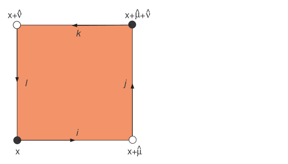
Figure 2: The plaquette corresponding to the variable $\Big{(}U_{\mu\nu}(x)\Big{)}_{ijkl}$ for $\mu\neq\nu$. The Chan-Paton indices are assigned on each link (1-simplex) as $i,j,k,l=1,\cdots,N$.

Notice that ordering of both the directional indices $\mu,\nu$ and the color indices $i,j,k,l$ are reversed by the complex conjugation.

We also define a gauge transformation rule as

$$\Big{(}U_{\mu\nu}(x)\Big{)}_{ijkl}\quad \rightarrow \sum_{i^{\prime},j^{\prime},k^{\prime},l^{\prime}}\Big{(}V_{\mu}(x)\Big{)}_{ii^{\prime}}\Big{(}V_{\nu}(x+\hat{\mu})\Big{)}_{jj^{\prime}}\Big{(}U_{\mu\nu}(x)\Big{)}_{i^{\prime}j^{\prime}k^{\prime}l^{\prime}}\Big{(}V_{\mu}(x+\hat{\nu})^{\dagger}\Big{)}_{k^{\prime}k}\Big{(}V_{\nu}(x)^{\dagger}\Big{)}_{l^{\prime}l}$$ (3.6)

$$\equiv \Big{(}(V_{\mu}\cdot V_{\nu}\cdot U_{\mu\nu}\cdot V_{\mu}^{\dagger}\cdot V_{\nu}^{\dagger})(x)\Big{)}_{ijkl},$$

where $V_{\mu}(x)$ are gauge transformation functions valued in U($N$) group, obeying $V_{\mu}(x)V_{\mu}^{\dagger}(x)={\bf 1}_{N}$. It is easy to see that ${\cal U}[C_{\mu\nu\lambda}(x)]$ in the action $S$ is associated to a 3-simplex (cube) as in Fig. 3, and invariant under the gauge transformation Eq.(3.6).

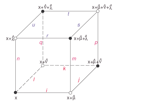
Figure 3: Chan-Paton factor assignment for the cube corresponding to ${\cal U}[C_{\mu\nu\lambda}(x)]$ in Eq.(3.4).

3.2 compactness conditions

In Wegner-Wilson-Polyakov lattice gauge theory, the link variables $(U_{\mu}(x))_{ij}$ are assumed compact, as defined via the conditions

$$\sum_{j=1}^{N}\Big{(}U_{\mu}(x)\Big{)}_{ij}\Big{(}U_{\mu}(x)\Big{)}^{*}_{i^{\prime}j}=\delta_{ii^{\prime}}\quad{\rm and}\quad\sum_{i=1}^{N}\Big{(}U_{\mu}(x)\Big{)}_{ij}\Big{(}U_{\mu}(x)\Big{)}^{*}_{ij^{\prime}}=\delta_{jj^{\prime}}.$$ (3.7)

It means that $(U_{\mu}(x))_{ij}$ are represented as $(N\times N)$ unitary matrices of the Lie group U($N$).

Likewise, we shall be restricting the configuration space of the plaquette variables $(U_{\mu\nu}(x))_{ijkl}$ to be compact. In the present case, however, there are four viable definitions of the compactness for plaquette variables. The first one, which we call as ‘rank-$N^{3}$ class’ is defined by

$$\mbox{rank-$N^{3}$}:\quad\sum_{l}\Big{(}U_{\mu\nu}(x)\Big{)}_{ijkl}\Big{(}U_{\mu\nu}(x)\Big{)}^{*}_{i^{\prime}j^{\prime}k^{\prime}l} = \frac{1}{N}\delta_{ii^{\prime}}\delta_{jj^{\prime}}\delta_{kk^{\prime}}$$

$$\sum_{k}\Big{(}U_{\mu\nu}(x)\Big{)}_{ijkl}\Big{(}U_{\mu\nu}(x)\Big{)}^{*}_{i^{\prime}j^{\prime}kl^{\prime}} = \frac{1}{N}\delta_{ii^{\prime}}\delta_{jj^{\prime}}\delta_{ll^{\prime}}$$

$$\sum_{j}\Big{(}U_{\mu\nu}(x)\Big{)}_{ijkl}\Big{(}U_{\mu\nu}(x)\Big{)}^{*}_{i^{\prime}jk^{\prime}l^{\prime}} = \frac{1}{N}\delta_{ii^{\prime}}\delta_{kk^{\prime}}\delta_{ll^{\prime}}$$

$$\sum_{i}\Big{(}U_{\mu\nu}(x)\Big{)}_{ijkl}\Big{(}U_{\mu\nu}(x)\Big{)}^{*}_{ij^{\prime}k^{\prime}l^{\prime}} = \frac{1}{N}\delta_{jj^{\prime}}\delta_{kk^{\prime}}\delta_{ll^{\prime}}.$$

The factor $\frac{1}{N}$ in the right-hand side was introduced by taking an appropriate overall normalization of the plaquette variables $U_{\mu\nu}(x)$. All four conditions are necessary, else the discrete rotational symmetry of the hypercube lattice would not be warranted.

For ‘rank-$N^{2}$ classes’, there are two possible choices. We will label them as $N^{2}$(I) and $N^{2}$(II) classes. They are

$$\mbox{rank-$N^{2}$(I)}:\quad\sum_{k,l}\Big{(}U_{\mu\nu}(x)\Big{)}_{ijkl}\Big{(}U_{\mu\nu}(x)\Big{)}^{*}_{i^{\prime}j^{\prime}kl} = \delta_{ii^{\prime}}\delta_{jj^{\prime}}$$ (3.8)

$$\sum_{l,i}\Big{(}U_{\mu\nu}(x)\Big{)}_{ijkl}\Big{(}U_{\mu\nu}(x)\Big{)}^{*}_{ij^{\prime}k^{\prime}l} = \delta_{jj^{\prime}}\delta_{kk^{\prime}}$$ (3.9)

$$\sum_{i,j}\Big{(}U_{\mu\nu}(x)\Big{)}_{ijkl}\Big{(}U_{\mu\nu}(x)\Big{)}^{*}_{ijk^{\prime}l^{\prime}} = \delta_{kk^{\prime}}\delta_{ll^{\prime}}$$ (3.10)

$$\sum_{j,k}\Big{(}U_{\mu\nu}(x)\Big{)}_{ijkl}\Big{(}U_{\mu\nu}(x)\Big{)}^{*}_{i^{\prime}jkl^{\prime}} = \delta_{ii^{\prime}}\delta_{ll^{\prime}},$$ (3.11)

and

$$\mbox{rank-$N^{2}$(II)}:\quad\sum_{j,l}\Big{(}U_{\mu\nu}(x)\Big{)}_{ijkl}\Big{(}U_{\mu\nu}(x)\Big{)}^{*}_{i^{\prime}jk^{\prime}l} = \delta_{ii^{\prime}}\delta_{kk^{\prime}}$$

$$\sum_{i,k}\Big{(}U_{\mu\nu}(x)\Big{)}_{ijkl}\Big{(}U_{\mu\nu}(x)\Big{)}^{*}_{ij^{\prime}kl^{\prime}} = \delta_{jj^{\prime}}\delta_{ll^{\prime}},$$

respectively.

Finally, there is the ‘rank-$N$ class’, defined by

$$\mbox{rank-$N$}:\quad\sum_{j,k,l}\Big{(}U_{\mu\nu}(x)\Big{)}_{ijkl}\Big{(}U_{\mu\nu}(x)\Big{)}^{*}_{i^{\prime}jkl} = N\delta_{ii^{\prime}}$$ (3.13)

$$\sum_{k,l,i}\Big{(}U_{\mu\nu}(x)\Big{)}_{ijkl}\Big{(}U_{\mu\nu}(x)\Big{)}^{*}_{ij^{\prime}kl} = N\delta_{jj^{\prime}}$$ (3.14)

$$\sum_{l,i,j}\Big{(}U_{\mu\nu}(x)\Big{)}_{ijkl}\Big{(}U_{\mu\nu}(x)\Big{)}^{*}_{ijk^{\prime}l} = N\delta_{kk^{\prime}}$$ (3.15)

$$\sum_{i,j,k}\Big{(}U_{\mu\nu}(x)\Big{)}_{ijkl}\Big{(}U_{\mu\nu}(x)\Big{)}^{*}_{ijkl^{\prime}} = N\delta_{ll^{\prime}}.$$ (3.16)

Notice that each conditions are related by lattice rotational symmetry, based on relation to the classical continuum limit. The four classes of compactness conditions are depicted geometrically in Fig.4.

Figure 4: Four classes of compactness conditions: (a) rank-$N^{3}$ conditions, (b) rank-$N^{2}$(I) conditions, (c) rank-$N^{2}$(II) conditions, (d) rank-$N$ conditions. Horizontal and vertical directions refer to $\hat{\mu}$ and $\hat{\nu}$, respectively. Chan-Paton indices at each overlapping edge are summed over.

Let us define the configuration space of the plaquette variables obeying these conditions as ${\mathbb{X}}_{N^{3}},{\mathbb{X}}_{N^{2}{\rm(I)}},{\mathbb{X}}_{N^{2}{\rm(II)}}$, and ${\mathbb{X}}_{N}$, respectively. Obviously,

$${\mathbb{X}}_{N^{3}}\quad\subset\quad{\mathbb{X}}_{N^{2}{\rm(I)}}\quad\mbox{and}\quad{\mathbb{X}}_{N^{2}{\rm(II)}}\quad\subset\quad{\mathbb{X}}_{N}.$$

It thus seems that four inequivalent definition of the theory exists at the quantum level.

Not all of them seem, however, physically acceptable. A condition we may impose is that the plaquette variables with a given compactness condition are always reducible to the link variables in a suitably prescribed limit. For example, consider ‘dimensional reduction’ of, say, the $d$-th direction with truncating the degrees of freedom of the internal indices as

$$(U_{d\mu}(x))_{ijkl}\Rightarrow\delta_{jl}(U_{\mu}(x))_{ik},\quad(U_{\mu d}(x))_{ijkl}\Rightarrow\delta_{ik}(U_{\mu}(x)^{\dagger})_{jl},\quad(U_{dd}(x))_{ijkl}\Rightarrow\delta_{ik}\delta_{jl},\qquad$$ (3.17)

where $x=(x^{1},\cdots,x^{d-1})$. This is a procedure of the standard dimensional reduction accompanied with a truncation of the internal degrees of freedom transforming as adjoint representation of $V_{\mu}(x)$. Then, $(U_{\mu}(x))_{ik}$ represents a link variable in Wilson’s lattice gauge theory as in Fig. 5 obeying the standard gauge transformation rule

$$U_{\mu}(x)\rightarrow V(x)U_{\mu}(x)V(x+\hat{\mu})^{\dagger},\qquad V(x)\in{\rm U}(N).$$

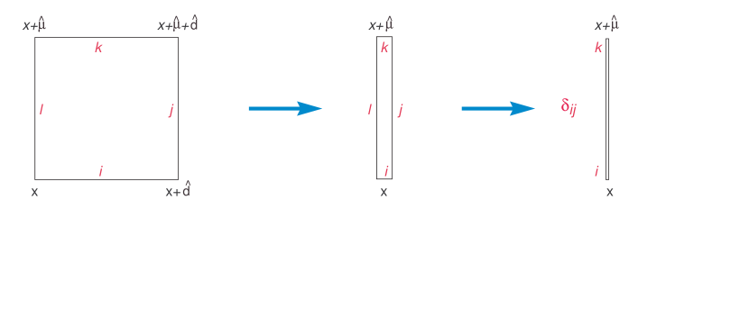
Figure 5: The plaquette variable $(U_{d\mu}(x))_{ijkl}$ reduces a variable on the link $(x,x+\hat{\mu})$ by truncating the degrees of freedom of the indices $j$, $l$ after the dimensional reduction with respect to the $d$-th direction,

In the lattice dimensional reduction, the tensor gauge theory action Eq.(3.1) is reduced to the Wilson’s action. We require that the compactness conditions are consistent with Eq.(3.7) under the reduction Eq.(3.17). As demonstrated in Appendix A, it is easy to see that the conditions of rank-$N^{3}$ and -$N^{2}$(II) are ruled out, and that the remaining two, rank-$N^{2}$(I) and rank-$N$ conditions, are consistent.

Henceforth, in this paper, we will consider the two classes for the compactness conditions: rank-$N^{2}$(I) conditions and rank-$N$ conditions. In the rest of this paper, we consider exclusively the rank-$N^{2}$(I) class. As will become clearer, this class of theory yields a physically meaningful classical continuum limit under the standard dimensional reduction keeping all the internal indices. For the rank-$N$ case, discussions are devoted to Appendix B. It turns out not to lead to a physically meaningful continuum classical theory after the dimensional reduction. As such, we conclude that consistency with the Yang-Mills theory via the dimensional reduction and the continuum limit therein singles out the rank $N^{2}$(I) class as the only physically meaningful compactness condition.

The partition function is defined as

$$Z\equiv\int{\cal D}U\,e^{-S},\qquad{\cal D}U\equiv\prod_{\{x\}}\prod_{\mu,\nu}[{\rm d}U_{\mu\nu}(x)],$$ (3.18)

where the measure $[{\rm d}U_{\mu\nu}(x)]$ is induced by the norm:

$$||\delta U_{\mu\nu}(x)||^{2}\equiv\sum_{i,j,k,l}\Big{(}\delta U_{\mu\nu}(x)\Big{)}_{ijkl}\Big{(}\delta U_{\mu\nu}(x)\Big{)}_{ijkl}^{*},$$

and the normalization is taken as $\int\,[{\rm d}U_{\mu\nu}(x)]=1$. It is readily seen that the norm is gauge invariant. So is the measure defined from it as well. For $N=1$ case, it coincides with the formulation of compact U(1) two-form tensor gauge theory on a lattice [21].

4 Relation to Dynamical Quantum Yang-Baxter Maps

In the previous section, we formulated lattice approach of nonabelian tensor gauge theory. The dynamical variables are elementary plaquettes, which carries not only spacetime orientation indices but also ‘color’ indices attached on four links around each elementary plaquette.

Before proceeding further, in this section, we point out the lattice theory is closely related to so-called dynamical quantum Yang-Baxter maps [28]. To appreciate possible connection most transparently, let us first consider ground-states, equivalently, saddle points of the lattice action. From Eq.(3.4), we see that the ground-states are characterized by the condition

$$\Big{(}U_{\mu\nu}(x)\cdot U_{\nu\lambda}(x)\cdot U_{\lambda\mu}(x)\Big{)}_{kqmjur}=\Big{(}U_{\lambda\mu}(x+\hat{\nu})\cdot U_{\nu\lambda}(x+\hat{\mu})U_{\mu\nu}(x+\hat{\lambda})\Big{)}_{kqmjur}\ ,$$ (4.1)

where left- and right-hand sides are abbreviations of

$$\Big{(}U_{\mu\nu}(x)\Big{)}_{ijkl}\Big{(}U_{\nu\lambda}(x)\Big{)}_{lqun}\Big{(}U_{\lambda\mu}(x)\Big{)}_{nrmi}$$

$$\Big{(}U_{\lambda\mu}(x+\hat{\nu})\Big{)}_{kptq}\Big{(}U_{\nu\lambda}(x+\hat{\mu})\Big{)}_{mspj}\Big{(}U_{\mu\nu}(x+\hat{\lambda})\Big{)}_{utsr}\,$$ (4.2)

respectively. This is a set of cubic algebraic relations among the elementary plaquette variables at each lattice sites $x$ and orientations of each cube. We shall make connection with the dynamical quantum Yang-Baxter maps progressively, first taking all plaquette variables constant valued and then taking account of dependence to the lattice sites and orientations.

Denote by $[x;\hat{\mu}\hat{\nu}\hat{\lambda}]$ an elementary cube based at $x$ and oriented along $\hat{\mu},\hat{\nu},\hat{\lambda}$ directions. Consider on the elementary cube a colored open string whose endpoints are fixed at mutually antipodal vertices. We can define the holonomy around the elementary cube by lassoing the string around the cube once, viz. nonabelian holonomy under parallel transport of the string around a closed manifold of ${\mathbb{S}}^{2}$ topology. The operation involves six plaquette moves on the cube: three plaquette moves plus their conjugate ones. Each set of three moves altogether is a map ${\cal X}\otimes{\cal X}\otimes{\cal X}\rightarrow{\cal X}\otimes{\cal X}\otimes{\cal X}$, thus carries 6 indices. This then defines the Yang-Baxter map and the curvature is measured by a ‘deformation’ of the Yang-Baxter equation:

$$U_{\mu\nu}U_{\nu\lambda}U_{\mu\lambda}=e^{ia^{3}H_{\mu\nu\lambda}}U_{\mu\lambda}U_{\nu\lambda}U_{\mu\nu},$$

for each elementary cube $[x;\hat{\mu}\hat{\nu}\hat{\lambda}]$. We immediately notice that the standard quantum Yang-Baxter equation corresponds to the equation for flat two-form connection, viz. vanishing parallel transport.

The way the plaquette variables are ordered is not arbitrary. Rather, it is intrinsically related to the way we define the parallel transport in terms of ‘lassoing’ the string. To see this, start with an ‘open’ string whose two endpoints are held fixed at the two oppositely diagonal vertices. It extends over three links, one per each directions of the cube. By a forward ‘move’, we define parallel transport of two adjacent links across the plaquette the two links belong to. We then see that succession of the moves ought to be such that the first three moves and the next three moves involve are oppositely ordered. In Fig.6, for instance, the string initially along the lower half cuts (composed of three links) the cube into two pieces. We first move the string across the lower half plaquettes of the cube: after move in the order of $[\mu\nu]$, $[\nu\lambda]$ and $[\mu\lambda]$ plaquettes, the string is now located at the along the upper cut (composed of three links).

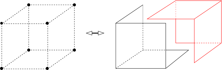
Figure 6: Quantum Yang-Baxter interpretation of holonomy around the cube.

The result of these moves is represented by

$$U_{\mu\nu}U_{\nu\lambda}U_{\mu\lambda}.$$

We then continue the move through the upper half plaquettes of the cube. In this case, the move is again in the order of $[\mu\nu]$, $[\nu\lambda]$ and $[\mu\lambda]$, but in the transposed orientation in each plaquette. The result of these moves is represented by

$$U^{\dagger}_{\mu\nu}U^{\dagger}_{\nu\lambda}U^{\dagger}_{\mu\lambda}.$$

Thus, putting togeter the two set of operations, a complete lassoing of the cube by a string is given by

$$U_{\mu\nu}U_{\nu\lambda}U_{\mu\lambda}U^{\dagger}_{\mu\nu}U^{\dagger}_{\nu\lambda}U^{\dagger}_{\mu\lambda},$$ (4.3)

and is precisely the holonomy of the antisymmetric tensor potential.

So far, we suppressed dependence of the elementary plaquette variables on lattice sites $x$ and orientations. Once we reinstate their dependence, the Yang-Baxter maps become enormously complicated. The dependence on lattice sites $x$ and on orientations of elementary cubes is not arbitrary, however. In particular, orientation of elementary plaquettes is closely tied with directional dependence. Remarkably, we see that these dependences are put together into the so-called dynamical quantum Yang-Baxter equations [dynamicalQYB] obeying:

$$U_{\mu\nu}(g-h^{\lambda})U_{\mu\lambda}(g)U_{\nu\lambda}(g-h^{\mu})=U_{\nu\lambda}(g)U_{\mu\lambda}(g+h^{\nu})U_{\mu\nu}(g).$$ (4.4)

Here, $g$ is an element of a Lie algebra ${\cal G}$ and $h$ is an element of its Cartan subalgebra. Then, making the expansion

$$U_{\mu\nu}=1+\hbar B_{\mu\nu}(h)+{\cal O}(\hbar^{2})$$ (4.5)

for an expansion parameter $\hbar$, we find that the leading-order contribution is given by

$${\rm d}_{\mu}B_{\nu\lambda}+{\rm d}_{\nu}B_{\lambda\mu}+{\rm d}_{\lambda}B_{\mu\nu}-[B_{\mu\nu},B_{\nu\lambda}]-[B_{\nu\lambda},B_{\lambda\mu}]-[B_{\lambda\mu},B_{\mu\nu}]=0,$$ (4.6)

where the derivative ${\rm d}_{\mu}$ is defined as

$${\rm d}_{\mu}={\bf e}^{(\mu)}\cdot{\partial\over\partial{\bf e}}$$ (4.7)

for the Cartan subalgebra of the Lie algebra ${\mathcal{G}}$ over ${\mathbb{C}}$. The left-hand side of Eq.(4.6) takes precisely the structure we may interpret as the nonabelian tensor field strength. So, we see that the dynamical quantum Yang-Baxter equation is the equation for vanishing field strength over the base manifold spanned by the Cartan subalgebra of $\mathcal{G}$.

5 Parametrization of Plaquette Variables

To proceed further, we will need to parametrize the plaquette variables $\left(U_{\mu\nu}(x)\right)_{ijkl}$ that satisfies the compactness conditions. In this section, we will construct explicitly a parametrization for the plaquette variables defined by the rank-$N^{2}$(I) compactness conditions Eq.(3.8-3.11).

5.1 Lax pair ansatz

Among the compactness conditions Eqs.(3.8 – 3.11), Eqs.(3.8, 3.10) imply that the plaquette variable $\left(U_{\mu\nu}(x)\right)_{ijkl}$ is a U($N^{2}$) matrix with respect to $(i,j)$ and $(k,l)$ pair of indices, referred as row and column indices. Likewise, Eqs.(3.9, 3.11) imply the same but now with respect to $(l,i)$ and $(j,k)$ pairs, identified as row and column indices. From these two requirements, we assume that $\left(U_{\mu\nu}(x)\right)_{ijkl}$, viewed as $(N^{2}\times N^{2})$ matrices, are projected onto a direct product of two matrices where the one acts on the indices, $i$ and $k$, and the other on $j$ and $l$ . Therefore, the plaquette variables are parametrizable as

$$\Big{(}U_{\mu\nu}(x)\Big{)}_{ijkl}:=\Big{(}W_{\mu\nu}(x)\Big{)}_{ik}\Big{(}\widetilde{W}_{\mu\nu}(x)\Big{)}_{jl},$$ (5.1)

viz. as a direct product of $W_{\mu\nu}(x)$ and $\widetilde{W}_{\mu\nu}(x)$ belonging to U($N)\times\widetilde{\rm U}(N)$.

The two matrices are not independent. The charge-conjugation relation Eq.(3.5) imposes that U($N)\simeq\widetilde{\rm U}(N)$, and that $\widetilde{W}_{\mu\nu}(x)=W_{\nu\mu}(x)^{\dagger}$. Thus, the plaquette variable is parametrizable in terms of U($N$) matrices $U^{(\mu)}_{\nu}(x)\equiv W_{\mu\nu}(x)$ as

$$\Big{(}U_{\mu\nu}(x)\Big{)}_{ijkl}=\Big{(}U^{(\mu)}_{\nu}(x)\Big{)}_{ik}\Big{(}U^{(\nu)\dagger}_{\mu}(x)\Big{)}_{jl}.$$ (5.2)

Notice that the diagonal U(1) part of $U^{(\mu)}_{\nu}(x)$ for either $\mu<\nu$ or $\mu>\nu$ are redundant for parametrizing the plaquette variable. Fortuituously, these extra U(1)’s do not interact with the rest, so they will be mod out straightforwardly. The gauge transformation of Eq.(3.6) gives rise to gauge transformation of $U^{(\mu)}_{\nu}(x)$ as

$$\Big{(}U^{(\mu)}_{\nu}(x)\Big{)}_{ik}\longrightarrow\sum_{i^{\prime},k^{\prime}=1}^{N}\Big{(}V_{\mu}(x)\Big{)}_{ii^{\prime}}\Big{(}U^{(\mu)}_{\nu}(x)\Big{)}_{i^{\prime}k^{\prime}}\Big{(}V_{\mu}^{\dagger}(x+\widehat{\nu})\Big{)}_{k^{\prime}k}.$$ (5.3)

We are thus parametrizing the plaquette variable as a square of $d$-species of U($N$) link variables, $U^{(\mu)}_{\nu}(x)$ with $\mu=1,\cdots,d$, each of which transforms as an adjoint under the gauge transformation $V_{\mu}(x)$. Intuitively, the newly introduced link variables $U^{(\mu)}_{\nu}$ in Eq.(5.2) are interpretable as the variables residing on two ‘dual’ links of the original plaquette, as depicted in Fig.7.

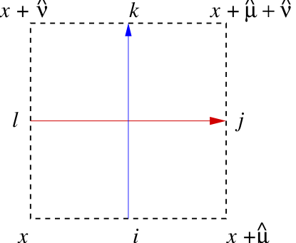
Figure 7: Parametrization of the plaquette variable $\left(U_{\mu\nu}(x)\right)_{ijkl}$ (the dashed lines) in terms of ‘dual’ links (the solid lines). The $d$-dimensional link variables $(U^{(\mu)}_{\nu}(x))_{ik}$, $(U^{(\nu)}_{\mu}(x)^{\dagger})_{jl}$ can be associated with the ‘dual’ links.

Actually, the dual lattice interpretation extends further. In terms of the newly introduced link variables $U^{(\mu)}_{\nu}(x)$, the gauge-invariant cube of the plaquette variables ${\cal U}[C_{\mu\nu\lambda}(x)]$ in Eq.(3.4) are expressible as a triple product of ‘dual’ plaquette, as depicted in Fig.8, and becomes

$${\cal U}[C_{\mu\nu\lambda}(x)]={\cal U}^{(\mu)}[P_{\nu\lambda}(x)]\,{\cal U}^{(\nu)}[P_{\lambda\mu}(x)]\,{\cal U}^{(\lambda)}[P_{\mu\nu}(x)],$$ (5.4)

where the $d$-species of ‘dual’ plaquette ${\cal U}^{(\mu)}$ are

$${\cal U}^{(\mu)}[P_{\nu\lambda}(x)]\equiv{\rm tr}\left[U^{(\mu)}_{\nu}(x)\,U^{(\mu)}_{\lambda}(x+\hat{\nu})\,U^{(\mu)^{\dagger}}_{\nu}(x+\hat{\lambda})\,U^{(\mu)^{\dagger}}_{\lambda}(x)\right].$$ (5.5)

Here, ‘tr’ refers to the trace operation with respect to $(N\times N)$ matrix indices of the dual link variables.

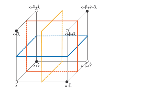
Figure 8: The original cube corresponding to ${\cal U}[C_{\mu\nu\lambda}(x)]$ (the dashed line) and the three ‘dual’ plaquettes ${\cal U}^{(\mu)}[P_{\nu\lambda}(x)]$, ${\cal U}^{(\nu)}[P_{\lambda\mu}(x)]$, ${\cal U}^{(\lambda)}[P_{\mu\nu}(x)]$ (the solid lines) for the case $\mu$, $\nu$, $\lambda$ all different.

Putting together, the nonabelian tensor gauge theory obeying the compactness conditions Eqs.(3.8 – 3.11) is defined by the partition function:

$$Z_{\rm tensor}\equiv\int[{\cal D}U]\,\exp(-S_{\rm tensor}),$$ (5.6)

where the action is

$$S_{\rm tensor}=-\beta\sum_{\{x\}}{\sum}_{\mu,\,\nu,\,\lambda=1}^{d}{}^{\prime}\hskip 28.45274pt\mbox{Re }\Big{(}{\cal U}^{(\mu)}[P_{\nu\lambda}(x)]\,{\cal U}^{(\nu)}[P_{\lambda\mu}(x)]\,{\cal U}^{(\lambda)}[P_{\mu\nu}(x)]-N^{3}\Big{)}$$ (5.7)

and the integral measure

$${\cal D}U=\prod_{\{x\}}[{\rm d}U(x)]\qquad\mbox{where}\qquad[{\rm d}U(x)]=\prod_{\mu,\,\nu=1}^{d}{}^{\prime}\hskip 5.69054pt[{\rm d}U^{(\mu)}_{\nu}(x)]/{\rm Vol}\left({\rm U}(1)^{d(d-1)/2}\right)$$ (5.8)

is given in terms of U$(N)$-invariant Haar measure  $[{\rm d}U^{(\mu)}_{\nu}(x)]$ of the dual link variables. The prime $(^{\prime})$ in the sum in Eq.(5.9) refers to summing over all nondegenerate plaquette orientations. Likewise, the prime $(^{\prime})$ in the product in Eq.(5.10) refers to integrating over all nondegenrate dual link variables. Notice that we eliminated the aforementioned over-counting in $U^{(\mu)}_{\nu}(x)$ for $\mu<\nu$ or $\mu>\nu$ by dividing the volume of overall U$(1)^{d(d-1)/2}$ gauge groups.

5.2 classical continuum limit

Before proceeding further, we will study classical continuum limit of the action Eq.(5.9) and show that the continuum action is manifestly $d$-dimensional Lorentz invariant.

At this stage, we will make a slight generalization of the theory we have constructed by incorporating into the theory the variable $(U_{\mu\mu}(x))_{ijkl}$ which is associated a collapsed plaquette as in Fig. 9.

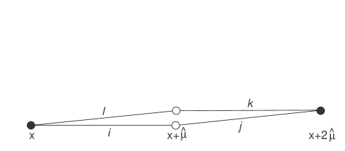
Figure 9: Degenerate class of plaquettes corresponding to the variable $\Big{(}U_{\mu\mu}(x)\Big{)}_{ijkl}$.

As will become clear momentarily, adding these variables are imperative in order to obtain a Lorentz invariant theory after taking a classical continuum limit. Still, the generalized theory is defined by the action Eq.(5.7) and the measure Eq.(5.8), where the sum over the Lorentz indices is unconstrained and the volume of overall groups is mod out for $d(d+1)$ U(1) gauge groups. Explicitly, the new action is defined by

$$S_{\rm tensor}=-\beta\sum_{\{x\}}{\sum}_{\mu,\,\nu,\,\lambda=1}^{d}\mbox{Re }\Big{(}{\cal U}^{(\mu)}[P_{\nu\lambda}(x)]\,{\cal U}^{(\nu)}[P_{\lambda\mu}(x)]\,{\cal U}^{(\lambda)}[P_{\mu\nu}(x)]-N^{3}\Big{)}\ ,$$ (5.9)

while the new functional integral measure is defined by

$${\cal D}U=\prod_{\{x\}}[{\rm d}U(x)]\qquad\mbox{where}\qquad[{\rm d}U(x)]=\prod_{\mu,\,\nu=1}^{d}[{\rm d}U^{(\mu)}_{\nu}(x)]/{\rm Vol}\left({\rm U}(1)^{d(d+1)/2}\right)\ .$$ (5.10)

Notice also that the gauge invariance and the parametrization of plaquette variable into split variables are straightforwardly extendible to degenerate variables as well.

To take continuum limit of the classical action, we expand the dual link variable $U^{(\mu)}_{\nu}(x)$ of U($N$) gauge group as 

$$U^{(\mu)}_{\nu}(x)=e^{ia^{2}A^{(\mu)}_{\nu}(x)}=1+ia^{2}A^{(\mu)}_{\nu}(x)-\frac{a^{4}}{2}\left(A^{(\mu)}_{\nu}(x)\right)^{2}+\cdots.$$ (5.11)

Here, $A^{(\mu)}_{\nu}(x)$ are $(N\times N)$ Hermitian matrices, where indices $\mu$ and $\nu$ transform as Lorentz vector indices. Accordingly, the U($N$)-invariant plaquette ${\cal U}^{(\mu)}[P_{\nu\lambda}(x)]$ is expandable as

$$U^{(\mu)}(P_{\nu\lambda}(x)) = N+ia^{3}{\rm tr}\Big{[}f^{(\mu)}_{\nu\lambda}(x)\Big{]}-\frac{1}{2}a^{6}{\rm tr}\Big{[}\left(f^{(\mu)}_{\nu\lambda}(x)\right)^{2}\Big{]}+{\cal O}(a^{7}),$$ (5.12)

$$f^{(\mu)}_{\nu\lambda}(x) \equiv \Delta_{\nu}A^{(\mu)}_{\lambda}(x)-\Delta_{\lambda}A^{(\mu)}_{\nu}(x),$$ (5.13)

where $\Delta_{\nu}$ denotes the lattice difference operator: $\Delta_{\nu}f(x)\equiv\frac{1}{a}(f(x+\hat{\nu})-f(x))$. Hence, the classical action is expanded as

$$S_{\rm tensor} = \frac{1}{2}\beta a^{6}\sum_{\{x\}}\sum_{\mu,\nu,\lambda=1}^{d}\Big{[}N^{3}H_{\mu\nu\lambda}^{\rm U(1)}(x)^{2}+N^{2}\,{\rm tr}\left\{\tilde{f}^{(\mu)}_{\nu\lambda}(x)^{2}+\tilde{f}^{(\nu)}_{\lambda\mu}(x)^{2}+\tilde{f}^{(\lambda)}_{\mu\nu}(x)^{2}\right\}\Big{]}+{\cal O}(a^{7})$$ (5.15)

$$= \frac{1}{2g^{2}}\int{\rm d}^{d}x\,\sum_{\mu,\nu,\lambda=1}^{d}\Big{[}N^{3}H_{\mu\nu\lambda}^{\rm U(1)}(x)^{2}+3N^{2}\,{\rm tr}\left(\tilde{f}^{(\mu)}_{\nu\lambda}(x)^{2}\right)\Big{]}+{\cal O}(a^{7})$$

in the classical continuum limit:

$$a\rightarrow 0\qquad{\rm and}\qquad\frac{1}{g^{2}}\equiv\beta a^{6-d}=\mbox{fixed}.$$ (5.16)

Here, we decomposed the field strength $f^{(\mu)}_{\nu\lambda}(x)$ into diagonal U(1) and traceless parts:

$$f^{(\mu)}_{\nu\lambda}(x)\equiv f^{(\mu)\,{\rm U(1)}}_{\nu\lambda}(x)\mathbb{I}_{N}+\tilde{f}^{(\mu)}_{\nu\lambda}(x)\qquad{\rm tr}\,\tilde{f}^{(\mu)}_{\nu\lambda}(x)=0.$$

The difference operators in Eq.(5.13) should be understood as ordinary derivatives in the continuum limit.

For the diagonal U(1) part, we have reproduced the totally antisymmetric 3-form field strength $H^{\rm U(1)}_{\mu\nu\lambda}=-f^{(\mu)\,{\rm U(1)}}_{\nu\lambda}(x)-f^{(\nu)\,{\rm U(1)}}_{\lambda\mu}(x)-f^{(\lambda)\,{\rm U(1)}}_{\mu\nu}(x)$. Thus, in the $N=1$ case, the result Eq.(5.15) reduces the previously known action of abelian tensor gauge theory. For U($N$), the 3-form field strength is constructed as an object carrying six color indices:

$$\Big{(}{\cal H}_{\mu\nu\lambda}(x)\Big{)}_{ijki^{\prime}j^{\prime}k^{\prime}}\equiv-\Big{(}f^{(\mu)}_{\nu\lambda}(x)\Big{)}_{ii^{\prime}}\delta_{jj^{\prime}}\delta_{kk^{\prime}}-\Big{(}f^{(\nu)}_{\lambda\mu}(x)\Big{)}_{jj^{\prime}}\delta_{kk^{\prime}}\delta_{ii^{\prime}}-\Big{(}f^{(\lambda)}_{\mu\nu}(x)\Big{)}_{kk^{\prime}}\delta_{ii^{\prime}}\delta_{jj^{\prime}}\ .$$

The field-strength is manifestly gauge invariant and has the symmetry properties:

$$\Big{(}{\cal H}_{\mu\nu\lambda}(x)\Big{)}_{ijki^{\prime}j^{\prime}k^{\prime}}=-\Big{(}{\cal H}_{\nu\mu\lambda}(x)\Big{)}_{jikj^{\prime}i^{\prime}k^{\prime}}=-\Big{(}{\cal H}_{\mu\lambda\nu}(x)\Big{)}_{ikji^{\prime}k^{\prime}j^{\prime}}=-\Big{(}{\cal H}_{\lambda\nu\mu}(x)\Big{)}_{kjik^{\prime}j^{\prime}i^{\prime}}\,,$$ (5.17)

meaning that ${\cal H}$ is antisymmetric under permutations with respect to the three sets of indices $(\mu,i,i^{\prime})$, $(\nu,j,j^{\prime})$, $(\lambda,k,k^{\prime})$. Utilizing these properties, the continuum action Eq.(5.15) is rewritable compactly as:

$$S=\frac{1}{2g^{2}}\int{\rm d}^{d}x\,\sum_{\mu,\nu,\lambda=1}^{d}{\rm Tr}_{N^{3}}\left({\cal H}_{\mu\nu\lambda}(x)\right)^{2},$$ (5.18)

where ‘${\rm Tr}_{N^{3}}$’ refers to the trace for $(N^{3}\times N^{3})$ matrices. It is defined for an generic element ${\cal A}_{ijki^{\prime}j^{\prime}k^{\prime}}$ as

$${\rm Tr}_{N^{3}}({\cal A})\equiv\ \sum_{i,j,k}\ {\cal A}_{ijkijk}.$$ (5.19)

Recall that, in defining the plaquette variables $U_{\mu\nu}(x)$, we have included those on degenerate plaquette $\mu=\nu$. Had one considered the lattice theory without them, the naive continuum action would be the same as Eq.(5.15) except that the summation over $\mu$, $\nu$, $\lambda$ is now restricted to the cases $\mu$, $\nu$, $\lambda$ all different. Then, the first term in Eq.(5.15) would still be Lorentz invariant, but the second term would not be so because the traceless part $\tilde{f}^{(\mu)}_{\nu\lambda}(x)$ is not totally antisymmetric with respect to $\mu$, $\nu$, $\lambda$. We have deliberately kept the degenerate plaquette variables so that Lorentz invariant continuum action Eq. (5.15) is obtainable.

The action Eq.(5.15) in the classical continuum limit is purely Gaussian. It does not necessarily mean that the corresponding quantum theory is free. For instance, as demonstrated in [19, 20, 21], $d=4$ tensor gauge theory of compact U(1) gauge group leads to charge confinement as a result of instanton effects. The result is in direct parallel to the situation [22] of $d=3$ compact U(1) gauge theory. Such effects are, however, entirely nonperturbative, having directly to do with the topology of the configuration space, and the continuum theory defined by the action Eq.(5.15) is perturbatively free. Given that the elementary dynamical variables are the link variables (defined on dual lattice), it is actually instructive to understand why the continuum theory is noninteracting. Recall that the gauge transformation function $V_{\mu}(x)$ in Eq.(5.3) is a Lorentz vector and is expandable as

$$V_{\mu}(x)=e^{ia\Lambda_{\mu}(x)}=1+ia\Lambda_{\mu}(x)-\frac{1}{2}a^{2}\left(\Lambda_{\mu}(x)\right)^{2}+\cdots,$$ (5.20)

with $\Lambda_{\mu}(x)$ being $(N\times N)$ Hermitian matrix-valued. Thus, in the continuum limit, the gauge transformation rule becomes abelian:

$$A^{(\mu)}_{\nu}(x)\rightarrow A^{(\mu)}_{\nu}(x)-\partial_{\nu}\Lambda_{\mu}(x).$$

This conclusion, despite being formulated in terms of the ‘dual’ link variables, marks the significant departure from the ordinary nonabelian lattice gauge theory. In the continuum theory, we are exploring small neighborhood of the identity in the lattice gauge transformation, and information of global structure of the group is lost. The global structure can be made visible by introducing a cutoff and considering the theory with compact variables, just like the lattice action Eq.(3.1) we started with.

6 Dimensional Reduction on the Lattice

Before proceeding further, we check an important consistency condition. We shall take dimensional reduction of the $d$-dimensional lattice tensor gauge theory and show that the theory Eq.(3.1) is reduced near the continuum limit to the $(d-1)$-dimensional lattice gauge theory coupled to an adjoint scalar field.

6.1 dimensional reduction for lattice vector fields

We first explain what we mean by ’dimensional reduction’ in lattice gauge theory. For definiteness, we shall consider the $d$-dimensional Wilson’s plaquette action:

$$S_{\rm YM} = -\beta\sum_{\{x\}}\sum_{\mu,\nu=1}^{d}{}^{\prime}\hskip 5.69054pt\mbox{Re}\,\Big{(}{\cal U}[P_{\mu\nu}(x)]-N\Big{)},$$ (6.1)

$${\cal U}[P_{\mu\nu}(x)] = {\rm tr}_{N}\left[U_{\mu}(x)U_{\nu}(x+\hat{\mu})U_{\mu}(x+\hat{\nu})^{\dagger}U_{\nu}(x)^{\dagger}\right],$$

where the summation of $\mu,\nu$ with the prime (^′) runs over the region $\mu\neq\nu$. The link variables $U_{\mu}(x)$ are $N\times N$ unitary matrices belonging to the gauge group G, satisfying Eq.(3.7). It is parametrized in terms of Lie-algebra-valued gauge potential $A_{\mu}(x)$ as

$$U_{\mu}(x)=e^{iaA_{\mu}(x)},$$ (6.2)

where again $a$ denotes the lattice spacing.

To consider dimensional reduction from $d$- to $(d-1)$-dimensions, we take the $d$-th lattice anisotropic, treat its lattice spacing $r$ much smaller than other lattice spacing $a$, and take the limit $r\rightarrow 0$. Then, $d$-dimensional hypercubic lattice collapses to $(d-1)$-dimensional lattice . Denote the $d$-th link variable $U_{d}(x)$ as

$$U_{d}(x)=e^{irA_{d}(x)},$$

while all others $U_{\mu}(x)$ ($\mu=1,\cdots,d-1$) remain unchanged in Eq.(6.2). Dimensional reduction then goes as follows. One picks up the lowest Kaluza-Klein modes (zero modes) with respect to the $d$-th lattice direction, so that $x$ now represents a site of $(d-1)$-dimensional lattice $(x_{1},\cdots,x_{d-1})$. In the limit $r\rightarrow 0$, $d$-th links are shrunken to a point, and the variable $U_{d}(x)$ is now associated with sites. We take the limit with the combination $\Phi(x)\equiv\frac{r}{a}A_{d}(x)$ kept fixed. The scalar field $\Phi(x)$ represents an adjoint scalar field carrying mass-dimension .

The dimensionally reduced lattice action becomes

$$S_{\rm YM}=-\beta\sum_{\{x\}}\sum_{\mu,\nu=1}^{d-1}{}^{\prime}\hskip 5.69054pt\mbox{Re}\,\Big{(}{\cal U}[P_{\mu\nu}(x)]-N\Big{)}-2\beta\sum_{\{x\}}\sum_{\mu=1}^{d-1}\mbox{Re}\,\Big{(}{\cal U}[P_{\mu d}(x)]-N\Big{)}.$$

After renaming

$$U(x)\equiv e^{ia\Phi(x)}=U_{d}(x),$$

the action in the classical continuum limit reproduces the known result of dimensional reduction:

$$S_{\rm YM} = \frac{1}{g_{\rm YM}^{2}}\int{\rm d}^{d-1}x\,{\rm tr}\left[\sum_{\mu,\nu=1}^{d-1}\frac{1}{4}\left(F_{\mu\nu}(x)\right)^{2}+\sum_{\mu=1}^{d-1}\frac{1}{2}\left(D_{\mu}\Phi(x)\right)^{2}\right],$$

$$F_{\mu\nu} = \partial_{\mu}A_{\nu}-\partial_{\nu}A_{\mu}+i[A_{\mu},A_{\nu}],\qquad D_{\mu}\Phi=\partial_{\mu}\Phi+i[A_{\mu},\Phi].$$ (6.4)

The limit $a\rightarrow 0$ is taken while holding $1/g_{\rm YM}^{2}\equiv 2\beta a^{4-(d-1)}$ fixed.

6.2 dimensional reduction for lattice tensor fields

By taking the same procedure, we now examine the dimensional reduction of our proposed lattice tensor gauge theory. Scaling the $d$-th dimension differently, we write the elementary plaquette variables as

$$U_{\mu\nu}(x) = I+ia^{2}B_{\mu\nu}(x)+\cdots,$$

$$U_{d\mu}(x) = I+iarB_{d\mu}(x)+\cdots,$$

$$U_{\mu d}(x) = I+iarB_{\mu d}(x)+\cdots,$$

$$U_{dd}(x) = I+ir^{2}B_{dd}(x)+\cdots,$$

with $\mu,\nu=1,\cdots,d-1$ and $I_{ijkl}=\delta_{ik}\delta_{jl}$. As $r\rightarrow 0$, extending the reasoning given above, we see that the variables $U_{d\mu}(x)$, $U_{\mu d}(x)$ become associated to links, while $U_{dd}(x)$ is associated to sites. They lead to vector and scalar fields on the $(d-1)$-dimensional hyper-cubic lattice, respectively. Both fields carry the mass-dimension one, and the limit $r\rightarrow 0$ ought to be taken with newly defined fields

$${\cal V}_{\mu}(x)\equiv rB_{d\mu}(x),\quad\tilde{{\cal V}}_{\mu}(x)\equiv rB_{\mu d}(x),\quad\Phi(x)\equiv\frac{r^{2}}{a}B_{dd}(x)$$

kept finite.

After the dimensional reduction, the gauge transformation rules become

$$\Big{(}U_{\mu}(x)\Big{)}_{ijkl} \equiv \Big{(}U_{d\mu}(x)\Big{)}_{ijkl}$$ (6.9)

$$\rightarrow \sum_{i^{\prime}j^{\prime}k^{\prime}l^{\prime}}\Big{(}V(x)\Big{)}_{ii^{\prime}}\Big{(}V_{\mu}(x)\Big{)}_{jj^{\prime}}\Big{(}U_{\mu}(x)\Big{)}_{i^{\prime}j^{\prime}k^{\prime}l^{\prime}}\Big{(}V(x+\hat{\mu})^{\dagger}\Big{)}_{k^{\prime}k}\Big{(}V_{\mu}(x)^{\dagger}\Big{)}_{l^{\prime}l},$$

$$\Big{(}\tilde{U}_{\mu}(x)\Big{)}_{ijkl} \equiv \Big{(}U_{\mu d}(x)\Big{)}_{ijkl}$$ (6.11)

$$\rightarrow \sum_{i^{\prime}j^{\prime}k^{\prime}l^{\prime}}\Big{(}V_{\mu}(x)\Big{)}_{ii^{\prime}}\Big{(}V(x+\hat{\mu})\Big{)}_{jj^{\prime}}\Big{(}\tilde{U}_{\mu}(x)\Big{)}_{i^{\prime}j^{\prime}k^{\prime}l^{\prime}}\Big{(}V_{\mu}(x)^{\dagger}\Big{)}_{k^{\prime}k}\Big{(}V(x)^{\dagger}\Big{)}_{l^{\prime}l},$$

$$\Big{(}U(x)\Big{)}_{ijkl} \equiv \Big{(}U_{dd}(x)\Big{)}_{ijkl}$$ (6.13)

$$\rightarrow \sum_{i^{\prime}j^{\prime}k^{\prime}l^{\prime}}\Big{(}V(x)\Big{)}_{ii^{\prime}}\Big{(}V(x)\Big{)}_{jj^{\prime}}\Big{(}U(x)\Big{)}_{i^{\prime}j^{\prime}k^{\prime}l^{\prime}}\Big{(}V(x)^{\dagger}\Big{)}_{k^{\prime}k}\Big{(}V(x)^{\dagger}\Big{)}_{l^{\prime}l},$$

where $V(x)$ is a U($N$) matrix-valued field residing at the site $x$. From the transformation rules, we see that $(U_{\mu}(x))_{ijkl}$ is a variable defined on the link $(x,x+\hat{\mu})$, transforming in adjoint representation of $V_{\mu}(x)$ and carrying additional internal symmetry group labelled by $j$, $l$ indices. Likewise, we see that $(\tilde{U}_{\mu}(x))_{ijkl}$ represents a variable defined on the link $(x+\hat{\mu},x)$, transforming in adjoint representation of $V_{\mu}(x)$ and carrying additional internal symmetry group labelled by $i$, $k$ indices. The variable $(U(x))_{ijkl}$ is defined at the site $x$, thus represents a scalar field transforming as (adjoint)$\times$(adjoint) of the additional internal symmetry group.

For the theory under consideration, since the plaquette variable is given in split form Eq.(5.2), the fields $U_{d\mu}$, $U_{\mu d}$, $U_{dd}$ are parametrizable as

$$\Big{(}U_{d\mu}(x)\Big{)}_{ijkl} = \Big{(}e^{iaA_{\mu}(x)}\Big{)}_{ik}\Big{(}e^{-iaA^{(\mu)}(x)}\Big{)}_{jl}\equiv\Big{(}U_{\mu}(x)\Big{)}_{ik}\Big{(}U^{(\mu)}(x)^{\dagger}\Big{)}_{jl},$$

$$\Big{(}U_{\mu d}(x)\Big{)}_{ijkl} = \Big{(}e^{iaA^{(\mu)}(x)}\Big{)}_{ik}\Big{(}e^{-iaA_{\mu}(x)}\Big{)}_{jl}\equiv\Big{(}U^{(\mu)}(x)\Big{)}_{ik}\Big{(}U_{\mu}(x)^{\dagger}\Big{)}_{jl},$$

$$\Big{(}U_{dd}(x)\Big{)}_{ijkl} = \,\Big{(}e^{+ia\varphi(x)}\Big{)}_{ik}\,\Big{(}e^{-ia\varphi(x)}\Big{)}_{jl}\equiv\Big{(}U(x)\Big{)}_{ik}\Big{(}U(x)^{\dagger}\Big{)}_{jl},$$

and the gauge transformation rules are

$$U_{\mu}(x) \rightarrow V(x)U_{\mu}(x)V(x+\hat{\mu})^{\dagger},$$

$$U^{(\mu)}(x) \rightarrow V_{\mu}(x)U^{(\mu)}(x)V_{\mu}(x)^{\dagger},$$

$$U(x) \rightarrow V(x)U(x)V(x)^{\dagger}.$$

In this case, the vector gauge fields with four indices $({\cal V}_{\mu})_{ijkl}$, $(\tilde{{\cal V}}_{\mu})_{ijkl}$ separate into the purely vector field degrees of freedom $(A_{\mu})_{ik}$ and the adjoint matter one $(A^{(\mu)})_{jl}$. Also, the scalar $(\Phi)_{ijkl}$ transforming as (adjoint)$\times$(adjoint) splits into two $\varphi$’s. In the classical continuum limit, the gauge transformation by $V_{\mu}(x)$ becomes invisible, so the field $(A^{(\mu)})_{jl}$ do not transform. Notice that, to fix redundant degrees of freedom of the overall U(1)’s in the split form, one may take

$${\rm tr}\,A^{(\mu)}(x)={\rm tr}\,\varphi(x)=0.$$ (6.18)

The dimensionally reduced action is then given by

$$S = -\beta\sum_{\{x\}}\sum_{\mu,\nu,\lambda=1}^{d-1}\,\mbox{Re}\left[{\cal U}[C_{\mu\nu\lambda}(x)]-N^{3}\right]$$ (6.20)

$$- 3\beta\sum_{\{x\}}\sum_{\mu,\nu=1}^{d-1}\,\mbox{Re}\left[{\cal U}[C_{\mu\nu d}(x)]-N^{3}\right]-3\beta\sum_{\{x\}}\sum_{\mu=1}^{d-1}\,\mbox{Re}\left[{\cal U}[C_{\mu dd}(x)]-N^{3}\right],$$

where the term $({\cal U}[C_{ddd}(x)]-N^{3})$ is suppressed because it vanishes trivially as a consequence of the split form of $U_{dd}(x)$. In the classical continuum limit, the first term becomes Eq.(5.18), but with $d$ replaced by $(d-1)$. For the second term, ${\cal U}[C_{\mu\nu d}(x)]$ consists of the three factors ${\cal U}^{(\mu)}[P_{\nu d}(x)]$, ${\cal U}^{(\nu)}[P_{d\mu}(x)]$, ${\cal U}^{(d)}[P_{\mu\nu}(x)]$. The last factor is nothing but the Wilson’s plaquette action giving

$${\cal U}^{(d)}[P_{\mu\nu}(x)]=N+ia^{2}{\rm tr}\left[\Delta_{\mu}A_{\nu}(x)-\Delta_{\nu}A_{\mu}(x)\right]+a^{4}{\rm tr}\left(-\frac{1}{2}F_{\mu\nu}(x)^{2}\right)+O(a^{5}).$$

The field strength $F_{\mu\nu}$ is defined as in Eq.(6.4). The first factor leads

$${\cal U}^{(\mu)}[P_{\nu d}(x)]=N+a^{4}{\rm tr}\left[-\frac{1}{2}(\Delta_{\nu}A^{(\mu)}(x))^{2}\right]+{\cal O}(a^{5}),$$

where the ${\cal O}(a^{2})$-contribution $ia^{2}{\rm tr}(\Delta_{\nu}A^{(\mu)}(x))$ vanishes due to Eq.(6.18). Thus, the second term in Eq.(6.20) becomes

$$-3\beta\sum_{\{x\}}\sum_{\mu,\,\nu=1}^{d-1}\,\mbox{Re}\left[{\cal U}[C_{\mu\nu d}(x)]-N^{3}\right]=3\beta a^{4}N^{2}\sum_{\{x\}}\sum_{\mu,\,\nu=1}^{d-1}\,{\rm tr}\left[\frac{1}{2}F_{\mu\nu}(x)^{2}+(\Delta_{\mu}A^{(\nu)}(x))^{2}\right]+{\cal O}(a^{5}).$$

Notice that the contribution is of order ${\cal O}(a^{4})$, overwhelming the ${\cal O}(a^{6})$ contribution of the first term consisting of the tensor fields alone. The third term is similarly computed to give the kinetic term of the adjoint matter $\varphi(x)$ at ${\cal O}(a^{4})$. It does not involve nonlinear coupling to the gauge field $A_{\mu}(x)$ or the scalar field $\varphi(x)$, since such couplings are either absent or are higher-orders in the continuum limit. Putting them together, we arrive at the classical continuum action

$$S=\frac{3N^{2}}{g_{\rm YM}^{2}}\int{\rm d}^{d-1}x\,{\rm tr}\left[\sum_{\mu,\,\nu=1}^{d-1}\left\{\frac{1}{2}\Big{(}F_{\mu\nu}(x)\Big{)}^{2}+\Big{(}\partial_{\mu}A^{(\nu)}(x)\Big{)}^{2}\right\}+\sum_{\mu=1}^{d-1}\Big{(}D_{\mu}\varphi(x)\Big{)}^{2}\right],$$ (6.21)

with $g^{-2}_{\rm YM}\equiv\beta a^{5-d}$ and the covariant derivative $D_{\mu}\varphi$ is defined as in Eq.(6.4). The action Eq.(6.21) describes the U($N$) gauge theory with adjoint matter, accompanied with $(d-1)$ copies of free decoupled fields.

The classical continuum action Eq.(6.21) is Lorentz invariant. We emphasize that this result is far from being obvious. Since the action Eq.(5.18) emerges from the ${\cal O}(a^{6})$ part of the lattice action, we need to keep the expansion Eq.(5.11) up to the $(A^{(\mu)}_{\nu})^{3}$ terms. On the other hand, to get the action Eq.(6.21) of the order ${\cal O}(a^{4})$, we need to expand $U_{\mu}$, $U^{(\mu)}$, $U$ up to $(A_{\mu})^{4}$, $(A^{(\mu)})^{4}$, $\varphi^{4}$, respectively. Because the mass dimension of fields is modified from taking the dimensional reduction (which involves taking factors of lattice spacing $a$ to the fields), the latter case needs information of one higher-order compared to the former case of $A^{(\mu)}_{\nu}$. Thus, it is highly nontrivial that the continuum limit Eq.(6.21) yields Lorentz invariant action Eq.(5.18).

7 Strong-Coupling Expansion

An attractive and promising feature of lattice formulation is the feasibility of exploring nonperturbative physics such as dynamical mass generation and confinement etc. One such method is the strong-coupling expansion, which was applied successfully for the Wilson’s lattice gauge theory, and amounts to expansions in powers of the inverse coupling. Strong-coupling expansions are defined intrinsically on a lattice and cannot be derived directly for the continuum counterpart. As such, one typically supplements the strong-coupling expansions with a suitable methods for extrapolating the results to the continuum limit. Nevertheless, even for finite lattice spacing, the strong-coupling expansions can lead to new insights by revealing dynamical mechanisms which are typical for strongly interacting continuum theories. With such motivation, in this section, we develop the method of strong-coupling expansions for the lattice tensor gauge theory.

Much as in Wilson’s lattice gauge theory, the lattice tensor gauge theory admits gauge-invariant, nonabelian Wilson surface operators – a direct counterpart of the Wilson loop operators. Correlation functions involving these Wilson surface operators are the main interest to us. Hence, we shall apply the strong-coupling expansion analysis to correlators involving $n$ Wilson surface operators for $n=0,1,2$, and extract information regarding free energy, internal energy, and surface tension.

Remarkably, we will find very distinctive behavior of the strong coupling expansion. For ordinary lattice gauge theory, it is well known that the strong-coupling expansion has a finite radius of convergence [29]. Here, for lattice tensor gauge theory, we will find that the strong-coupling expansion is not absolutely convergent but an asymptotic series in the large $N$ limit. As weak-coupling perturbation theories give rise to asymptotic series, we conjecture that strong-coupling expansion of the lattice tensor gauge theory at large $N$ is dual to an another, weakly coupled lattice theory.

7.1 gauge-fixing

On a lattice of finite volume and finite spacing, the total number and the domain of integration for plaquette variables are finite. Therefore, the functional integral is well defined even without gauge fixing. Still, for a given computation of physical quantities, it is often advantageous to fix a suitable gauge. We will make use of this gauge-fixing freedom such that some of the plaquette variables are set equal to a prescribed value. Recall that we have included in the set of elementary plaquette variables those associated with degenerate plaquette, $U^{(\mu)}_{\mu}(x)$. We found it convenient to use the gauge freedom and set them to unity, $U^{(\mu)}_{\mu}(x)=\mathbb{I}_{N}$ for all $x$. To show that this procedure is always possible, it suffices to find an appropriate gauge transformation function $V_{\mu}(x)$ such that

$$V_{\mu}(x)U^{(\mu)}_{\mu}(x)V_{\mu}(x+\mu)^{\dagger}=\mathbb{I}_{N}.$$

We find that

$$V_{\mu}(x)=\left\{\begin{array}[]{ll}\mathbb{I}_{N}&\mbox{for $x_{\mu}=0$}\\ \prod_{y=0}^{x_{\mu}}U^{(\mu)}_{\mu}(x_{1},\cdots,x_{\mu-1},y,x_{\mu+1},\cdots,x_{d})&\mbox{for $x_{\mu}>0$}\\ \prod_{y=-1}^{x_{\mu}}U^{(\mu)}_{\mu}(x_{1},\cdots,x_{\mu-1},y,x_{\mu+1},\cdots,x_{d})^{\dagger}&\mbox{for $x_{\mu}<0$}.\end{array}\right.$$ (7.4)

In the gauge choice $U^{(\mu)}_{\mu}(x)=1$, the lattice action Eq.(5.9) reduces to

$$S_{\rm tensor} = -\beta\sum_{\{x\}}\sum_{\mu,\,\nu,\,\lambda=1}^{d}{}^{\prime}\,\,\mbox{Re }\Big{(}{\cal U}^{(\mu)}[P_{\nu\lambda}(x)]\,{\cal U}^{(\nu)}[P_{\lambda\mu}(x)]\,{\cal U}^{(\lambda)}[P_{\mu\nu}(x)]-N^{3}\Big{)},$$ (7.5)

where the primed sum over the Lorentz indices runs over $\mu$, $\nu$, $\lambda$ all different.

Notice that the gauge-fixing we have made is partial: the action is still invariant under a class of gauge transformations $V_{\mu}(x)$ that leaves the gauge choice $U_{\mu}^{(\mu)}=1$ intact. Such gauge transformations are the ones independent of $x^{\mu}$ coordinates, since

$$V_{\mu}(x)V_{\mu}(x+\mu)^{\dagger}=1\quad\mbox{viz.}\quad V_{\mu}(x)=V_{\mu}(x+\mu).$$ (7.6)

Notice also that the gauge-fixing does not introduce any nontrivial Jacobian or Faddeev-Popov ghosts either.

7.2 character expansion

To proceed further for the strong-coupling expansion, we perform the character expansion [23]. The gauge-fixed action Eq.(7.5) is a triple product of U($N$) characters in fundamental representation. So, for $U,V,W\in$ U($N$), we expand as

$$\exp\Big{(}3\beta\,[\chi_{\Box}(U)\chi_{\Box}(V)\chi_{\Box}(W)]+{\rm c.c.}\Big{)}=\sum_{\tt R_{1},R_{2},R_{3}}C_{\tt R_{1},R_{2},R_{3}}(\beta)\chi_{\tt R_{1}}(U)\chi_{\tt R_{2}}(V)\chi_{\tt R_{3}}(W),$$ (7.7)

where $\chi_{\tt R}(U)$ refers to the character of the irreducible representation $\tt R$ of gauge group U($N$). The character of the complex conjugate representation $\tt\bar{R}$ is related to it as $\chi_{\tt\bar{R}}(U)=\chi^{*}_{\tt R}(U)=\chi_{\tt R}(U^{\dagger})$. For the trivial representation ${\tt R}=0$, $\chi_{0}(U)=1$, and, for the fundamental representation ${\tt R}=\Box$, $\chi_{\Box}(U)={\rm tr}\,U$. The sum over $\tt R_{1},R_{2},R_{3}$ in Eq.(7.7) is for all unitary irreducible representations of the gauge group U($N$). The expansion Eq.(7.7) shows that the expansion coefficient $C_{\tt R_{1},R_{2},R_{3}}(\beta)$ is totally symmetric under permutations of $\tt R_{1},R_{2},R_{3}$, and that $C_{\tt R_{1},R_{2},R_{3}}(\beta)=C_{\tt\bar{R}_{1},\bar{R}_{2},\bar{R}_{3}}(\beta)$.

Recall that the characters can split or join under the U($N$) group integrals as

$$\int[{\rm d}U]\,\chi_{\tt R}(UAU^{\dagger}B) = \frac{1}{d_{\tt R}}\,\chi_{\tt R}(A)\,\chi_{\tt R}(B),$$ (7.8)

$$\int[{\rm d}U]\,\chi_{{\tt R}_{1}}(UA)\,\chi_{{\tt R}_{2}}(U^{\dagger}B) = \delta_{{\tt R}_{1},{\tt R}_{2}}\,\frac{1}{d_{{\tt R}_{1}}}\,\chi_{{\tt R}_{1}}(AB).$$ (7.9)

Here, $d_{\tt R}=\chi_{\tt R}(1)$ denotes the dimension of the representation ${\tt R}$. For example, $d_{0}=1$, $d_{\Box}=d_{\frac{}{\Box}}=N$. The orthogonality relations of characters (the $A=B=1$ case in Eq.(7.9)), the inverse relation of Eq.(7.7) is readily obtainable:

$$C_{{\tt R}_{1}{\tt R}_{2}{\tt R}_{3}}=\int[{\rm d}U][{\rm d}V][{\rm d}W]\,\chi_{{\tt R}_{1}}(U)\,\chi_{{\tt R}_{2}}(V)\,\chi_{{\tt R}_{3}}(W)\,\exp\Big{(}3\beta\,[\chi_{\Box}(U)\chi_{\Box}(V)\chi_{\Box}(W)]+\,{\rm c.c.}\Big{)}.$$ (7.10)

Factoring out the contribution $C_{000}(\beta)$, we express Eq.(7.7) in a more convenient form

$$\exp\Big{(}\!3\beta\,[\chi_{\Box}(U)\chi_{\Box}(V)\chi_{\Box}(W)]+{\rm c.c.}\!\Big{)}=C_{000}(\beta)\left[1+\sum_{{\tt R}_{1},{\tt R}_{2},{\tt R}_{3}}^{\prime}\widetilde{C}_{{\tt R}_{1}{\tt R}_{2}{\tt R}_{3}}(\beta)\chi_{{\tt R}_{1}}(U)\chi_{{\tt R}_{2}}(V)\chi_{{\tt R}_{3}}(W)\!\right],$$ (7.11)

where $\widetilde{C}_{{\tt R}_{1}{\tt R}_{2}{\tt R}_{3}}(\beta)\equiv C_{{\tt R}_{1}{\tt R}_{2}{\tt R}_{3}}(\beta)/C_{000}(\beta)$, and the primed sum runs over all unitary irreducible representations except $({\tt R}_{1},{\tt R}_{2},{\tt R}_{3})=(0,0,0)$.

We have computed the character expansion coefficient $C_{000}(\beta)$ from Eq.(7.11) in Appendix D. The result is in power-series of $\beta$:

$$C_{000}(\beta)=\sum_{n=0}^{N}\,n!\,(3\beta)^{2n}+\sum_{n=N+1}^{\infty}\,(v_{n})^{3}\,n!\,(3\beta)^{2n}.$$ (7.12)

It shows that the expansion coefficient grows as $n!$ up to the ${\cal O}(\beta^{2N})$, and then decreases by the factor $0<v_{n}<1$. In Appendix D, we computed the first 20 and 50 terms for $N=2$ and 3 cases, respectively, and concluded from the result that the suppression by $(v_{n})^{3}$ is sufficient to render the power-series Eq.(7.12) convergent for finite $N$. It implies that the power-series expansion of $\widetilde{C}_{\Box\Box\Box}(\beta)$ is convergent as well:

$$\widetilde{C}_{\Box\Box\Box}(\beta) := \frac{1}{2}\frac{\partial}{\partial(3\beta)}\ln C_{000}(\beta)$$ (7.13)

$$= (3\beta)\left[1+3(3\beta)^{2}+13(3\beta)^{4}+71(3\beta)^{6}+461(3\beta)^{8}+\cdots\right].$$ (7.14)

For the second equality, we assumed $N\geq 5$.

Interestingly, the large-order behavior of the character expansion coefficients is quite different from that of Wilson’s lattice gauge theory. For the latter, the character expansion yields

$$\exp\Big{(}\gamma\,\chi_{\Box}(U)+{\rm c.c.}\Big{)}=\sum_{{\tt R}}C_{{\tt R}}(\gamma)\chi_{\tt R}(U),\qquad C_{\tt R}(\gamma)=\int[{\rm d}U]\,\chi_{\tt R}(U)\exp\Big{(}\gamma\chi_{\Box}(U)+{\rm c.c.}\Big{)}.$$

The character expansion coefficient $C_{0}(\gamma)$, which is the same as $z(\gamma)$ defined in Eq.(D.3), can be computed explicitly. We relegate details to appendix D and quote here the result from Eq.(D.15):

$$C_{0}(\gamma)=z(\gamma)=\sum_{n=0}^{N}\,\frac{\gamma^{2n}}{n!}+\sum_{n=N+1}^{\infty}\,\frac{v_{n}}{n!}\,\gamma^{2n}.$$ (7.15)

Here, the first $N$ terms coincide with those of $e^{\gamma^{2}}$, and the power-series converges for any value of $\gamma$.

Of notable situation is the large-$N$ limit. For Wilson’s lattice gauge theory, as is evident from Eq.(7.15), the first term with $N=\infty$ yields a convergent large-order behavior. For the lattice tensor gauge theory, however, Eq.(7.12) with $N=\infty$ is obviously divergent and is not even Borel summable. This imparts a significant departure of our lattice tensor gauge theory from Wilson’s lattice gauge theory. We will dwell on this issue further later in subsection 7.5.

7.3 partition function and free energy

For the gauge $U^{(\mu)}_{\mu}=1$, the gauge-fixed partition function is given by

$$Z = e^{-\beta N^{3}d(d-1)(d-2){\cal N}_{s}}\,{\cal Z}\,,$$

$${\cal Z} = \int{\cal D}^{\prime}U\,\prod_{\{x\}}\prod_{\mu<\nu<\lambda}\exp\Big{(}3\beta\,{\cal U}^{(\mu)}[P_{\nu\lambda}(x)]\,{\cal U}^{(\nu)}[P_{\lambda\mu}(x)]\,{\cal U}^{(\lambda)}[P_{\mu\nu}(x)]+\,{\rm c.c.}\Big{)},$$ (7.16)

where ${\cal N}_{s}$ refers to the total number of lattice sites, and the measure ${\cal D}^{\prime}U$ is the U($N$)-Haar measure for the regular plaquette variables $U^{(\mu)}_{\nu}(x)$ $(\mu\neq\nu)$. Here, we do not consider the volume factor of U(1) groups as in Eq.(5.10) since it merely produces an irrelevant constant factor independent of $\beta$ and $N$.

Once the expansion Eq.(7.11) is made for each cube, Eq.(7.16) can be written as

$${\cal Z}=\Big{(}C_{000}(\beta)\Big{)}^{\frac{1}{3!}d(d-1)(d-2){\cal N}_{s}}$$

(7.17)

$$\times\int{\cal D}^{\prime}U\,\prod_{\{x\}}\prod_{\mu<\nu<\lambda}\left[1+\!\!\!\sum_{{\tt R}_{1},{\tt R}_{2},{\tt R}_{3}}^{\prime}\,\,\tilde{C}_{{\tt R}_{1}{\tt R}_{2}{\tt R}_{3}}(\beta)\,\chi_{{\tt R}_{1}}\left(P^{(\mu)}_{\nu\lambda}(x)\right)\,\chi_{{\tt R}_{2}}\left(P^{(\nu)}_{\lambda\mu}(x)\right)\,\chi_{{\tt R}_{3}}\left(P^{(\lambda)}_{\mu\nu}(x)\right)\right].$$ (7.18)

Here, $P^{(\mu)}_{\nu\lambda}(x)$ denotes the plaquette $P_{\nu\lambda}(x)$ formed by the dual link variables carrying superscript $(\mu)$, viz. $P^{(\mu)}_{\nu\lambda}(x)=U^{(\mu)}_{\nu}(x)\,U^{(\mu)}_{\lambda}(x+\hat{\nu})\,U^{(\mu)}_{\nu}(x+\hat{\lambda})^{\dagger}\,U^{(\mu)}_{\lambda}(x)^{\dagger}$. The triple product of the characters in Eq.(7.18) corresponds to the elementary cube or triple product among its‘dual’ plaquettes (depicted in Fig. 8) carrying the representations ${\tt R}_{1},{\tt R}_{2},{\tt R}_{3}$. The integrals in Eq.(7.18) is carried out by making use of the integration formulas Eqs.(7.8, 7.9). Nontrivial contributions come from situations that elementary cubes, each of which are labelled by the representations ${\tt R}_{1},{\tt R}_{2},{\tt R}_{3}$ are glued together into three-dimensional closed manifolds on the lattice. Consider the simplest one of such cases. It is that eight cubes are glued together to form a manifold of ${\mathbb{S}}^{3}$ topology. An example of such a configuration consists of the following elementary cubes:

$$(1): \chi_{{\tt R}_{1}}\left(P^{(1)}_{23}(x)\right)\,\chi_{{\tt R}_{2}}\left(P^{(2)}_{31}(x)\right)\,\chi_{{\tt R}_{3}}\left(P^{(3)}_{12}(x)\right)$$ (7.19)

$$(2): \chi_{{\tt R}_{1}}\left(P^{(1)}_{32}(x+\hat{4})\right)\,\chi_{{\tt R}_{2}}\left(P^{(2)}_{13}(x+\hat{4})\right)\,\chi_{{\tt R}_{3}}\left(P^{(3)}_{21}(x+\hat{4})\right)$$ (7.20)

$$(3): \chi_{{\tt R}_{2}}\left(P^{(2)}_{43}(x)\right)\,\chi_{{\tt R}_{3}}\left(P^{(3)}_{24}(x)\right)\,\chi_{{\tt R}_{4}}\left(P^{(4)}_{23}(x)\right)$$ (7.21)

$$(4): \chi_{{\tt R}_{2}}\left(P^{(2)}_{34}(x+\hat{1})\right)\,\chi_{{\tt R}_{3}}\left(P^{(3)}_{41}(x+\hat{1})\right)\,\chi_{{\tt R}_{4}}\left(P^{(4)}_{32}(x+\hat{1})\right)$$ (7.22)

$$(5): \chi_{{\tt R}_{1}}\left(P^{(1)}_{34}(x)\right)\,\chi_{{\tt R}_{3}}\left(P^{(3)}_{41}(x)\right)\,\chi_{{\tt R}_{4}}\left(P^{(4)}_{31}(x)\right)$$ (7.23)

$$(6): \chi_{{\tt R}_{1}}\left(P^{(1)}_{43}(x+\hat{2})\right)\,\chi_{{\tt R}_{3}}\left(P^{(3)}_{14}(x+\hat{2})\right)\,\chi_{{\tt R}_{4}}\left(P^{(4)}_{13}(x+\hat{2})\right)$$ (7.24)

$$(7): \chi_{{\tt R}_{1}}\left(P^{(1)}_{42}(x)\right)\,\chi_{{\tt R}_{2}}\left(P^{(2)}_{14}(x)\right)\,\chi_{{\tt R}_{4}}\left(P^{(4)}_{12}(x)\right)$$ (7.25)

$$(8): \chi_{{\tt R}_{1}}\left(P^{(1)}_{24}(x+\hat{3})\right)\,\chi_{{\tt R}_{2}}\left(P^{(2)}_{41}(x+\hat{3})\right)\,\chi_{{\tt R}_{4}}\left(P^{(4)}_{21}(x+\hat{3})\right),$$ (7.26)

where each cube is represented in terms of characters of ‘dual’ plaquettes, and hermitian conjugation relations such as $P^{(\mu)}_{\nu\lambda}(x)^{\dagger}=P^{(\mu)}_{\lambda\nu}(x)$ are used repeatedly. The group integration then yields

$$\int[{\rm d}U]\,\mbox{(1)}\times\mbox{(2)}\times\mbox{(3)}\times\mbox{(4)}\times\mbox{(5)}\times\mbox{(6)}\times\mbox{(7)}\times\mbox{(8)}=\frac{1}{(d_{{\tt R}_{1}}d_{{\tt R}_{2}}d_{{\tt R}_{3}}d_{{\tt R}4})^{4}}.$$

Intuitively, the result can be understood in terms of the resulting three manifolds. Rewriting contribution of each representation as $d_{\tt R}^{-4}=d_{\tt R}^{2}\times d_{\tt R}^{-6}$, the power ‘2’ in the first factor is interpretable as the Euler characteristic of ${\mathbb{S}}^{2}$ made of six ‘dual’ plaquettes corresponding to $\chi_{\tt R}$, and the power ‘$-6$’ in the second factor is the correct normalization of $\chi_{\tt R}$ that permits ’t Hooft’s large-$N$ power counting. Summing over all possible representations of the cubes, the total contribution is given by

$$\sum_{{\tt R}_{1},{\tt R}_{2},{\tt R}_{3},{\tt R}_{4}}^{\prime}\hskip 17.07164pt\left(\frac{1}{d_{{\tt R}_{1}}d_{{\tt R}_{2}}d_{{\tt R}_{3}}d_{{\tt R}_{4}}}\right)^{4}\,\left(\widetilde{C}_{{\tt R}_{1}{\tt R}_{2}{\tt R}_{3}}(\beta)\widetilde{C}_{{\tt R}_{2}{\tt R}_{3}{\tt R}_{4}}(\beta)\widetilde{C}_{{\tt R}_{3}{\tt R}_{4}{\tt R}_{1}}(\beta)\widetilde{C}_{{\tt R}_{4}{\tt R}_{1}{\tt R}_{2}}(\beta)\right)^{2},$$ (7.27)

where the prime (^′) of the summation stands for excluding the term $({\tt R}_{1},{\tt R}_{2},{\tt R}_{3},{\tt R}_{4})=(0,0,0,0)$. The leading nonzero term comes from the case ${\tt R}_{1}={\tt R}_{2}={\tt R}_{3}={\tt R}_{4}=\Box$ and its complex conjugate, yielding $2(3\beta)^{8}/N^{16}$. The next order contribution comes from the case the representations involve identity or adjoint. Because $C_{0,0,{\rm ad}}(\beta)$, $C_{0,{\rm ad},{\rm ad}}(\beta)$, $C_{{\rm ad},{\rm ad},{\rm ad}}(\beta)$ all start with $(3\beta)^{2}$, it gives the contribution of ${\cal O}(\beta^{12})$. Therefore, we find the partition function in strong-coupling expansion as:

$${\cal Z} = \Big{(}C_{000}(\beta)\Big{)}^{\frac{1}{3!}d(d-1)(d-2){\cal N}_{s}}$$ (7.29)

$$\times\left[1+\frac{1}{4!}d(d-1)(d-2)(d-3){\cal N}_{s}\cdot\frac{2}{N^{16}}\,\Big{(}\widetilde{C}_{\Box\Box\Box}(\beta)\Big{)}^{8}+{\cal O}(\beta^{12})\right].$$

Here, as explained already, the series-expansion in $C_{{\tt R}_{1}{\tt R}_{2}{\tt R}_{3}}(\beta)$ represents sum over closed three-manifolds. Since terms higher-order in $C_{{\tt R}_{1}{\tt R}_{2}{\tt R}_{3}}(\beta)$ come from contractions among the same variables repeated many times, the power series of $3\beta$ in $C_{{\tt R}_{1}{\tt R}_{2}{\tt R}_{3}}(\beta)$ is interpretable as contributions of singular, degenerate closed three-manifolds.

7.4 Wilson surface observables

7.4.1 Nonabelian Wilson surfaces

We begin with a digression regarding nonabelian Wilson surfaces. It is normally considered that, for nonabelian 2-form gauge theory, Wilson surfaces are ill-defined. We now show that the no-go theorem is evaded for the class of nonabelian tensor gauge theory studied in this paper.

Consider the trace of parallel transport around a closed surface $\Sigma$ ($\partial\Sigma=0$):

$${\rm Tr}U(\Sigma)=\prod_{P\in\Sigma}U_{P}.$$

In general, the surface $\Sigma$ would be self-intersecting. We will call expectation value of such variables:

$${\cal W}(\Sigma)\equiv\langle{\rm Tr}U(\Sigma)\rangle,$$ (7.30)

as the Wilson surface observables, and expectation value of their products:

$${\cal W}(\Sigma_{1},\cdots,\Sigma_{n})\equiv\langle{\rm Tr}U(\Sigma_{1})\,{\rm Tr}U(\Sigma_{2})\,\cdots{\rm Tr}U(\Sigma_{n})\rangle$$ (7.31)

as Wilson surface correlators. The Wilson surface observables measure internal energy of the system, and the (connected components of) the correlators measure correlation length, mass gap, spectrum, etc.

Wilson surface observables constitute the fundamental basis of the system. Indeed, extending the argument of [31], one can assert that every gauge-invariant operator ${\cal O}$, which depends continuously on the plaquette variables can be approximated arbitrarily well by a power-series of the Wilson surface variables:

$${\cal O}\simeq\sum_{n\geq 0}\sum_{\{\Sigma_{n}\}}c(\Sigma_{1},\cdots,\Sigma_{n})\,{\rm Tr}U(\Sigma_{1})\cdots{\rm Tr}U(\Sigma_{n}).$$ (7.32)

An important feature of proposed nonabelian Wilson surface observables is that it bypasses folklore that such observables are afflicted by ordering ambiguity. For a Wilson surface observable of minimal size, viz. the one defined on a cube, we have already shown that there is no ambiguity. Could there be any ambiguity when the observables encompass cubes more than one? We will now argue that there is no ambiguity by illustrating a few nontrivial cases. The first one involves two cubes, as shown in the figure 10. Although there are two possible routes of color move across the plaquettes involved,

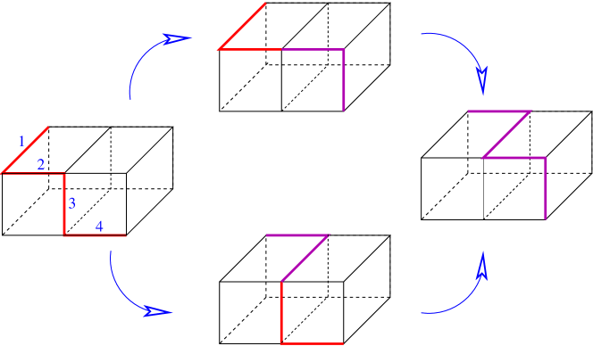
Figure 10: Two alternative routes around two disjoint plaquettes between two string configurations.

We can also illustrate our claim from more sophiscated string move in a given Wilson surface observable, as depicted in Fig.11.

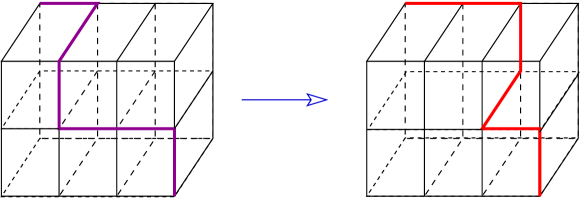
Figure 11: Two alternative routes around an elementary cube between two string configurations.

7.4.2 One-point correlator and internal energy

Having shown that nonabelian Wilson surface operators are well-defined physical observables, we now consider the simplest of these operators, taking a rectangular shape: $W_{x}(I,J,K)$ which represents a box with the positive orientation, composed by the three edges $(x,x+I\hat{1})$, $(x,x+J\hat{2})$, $(x,x+K\hat{3})$. It is constructed by tiling faces of the box with the plaquette variables $U_{\mu\nu}$. In computation of the vacuum expectation value $\langle W_{x}(I,J,K)\rangle$ in the strong coupling expansion, contributions correspond to various three-dimensional manifolds bounded by the box $W_{x}(I,J,K)$.

Let us begin with $\langle W_{x}(1,1,1)\rangle$. It is nothing but the internal energy and is computable as

$$\langle{W}_{x}(1,1,1)\rangle = \frac{3}{d(d-1)(d-2)}\frac{1}{{\cal N}_{s}}\,\frac{\partial}{\partial(3\beta)}\,\ln{\cal Z}$$ (7.33)

$$= \widetilde{C}_{\Box\Box\Box}(\beta)+2(d-3)\frac{1}{N^{16}}\left(\widetilde{C}_{\Box\Box\Box}(\beta)\right)^{7}+{\cal O}(\beta^{9}),$$ (7.34)

where the first term comes from the minimal volume configuration, and the second from elementary fluctuations consisting of seven cubes.

Extending the computation to general Wilson surface $\langle W_{x}(I,J,K)\rangle$, we find

$$\langle{W}_{x}(I,J,K)\rangle = \left(\frac{\widetilde{C}_{\Box\Box\Box}(\beta)}{N^{3}}\right)^{IJK}\hskip-17.07182pt\times N^{I+J+K}\left[1+2(d-3)IJK\frac{(\widetilde{C}_{\Box\Box\Box}(\beta))^{6}}{N^{16}}+{\cal O}(\beta^{8})\right].\hskip 14.22636pt$$ (7.35)

The leading contribution gives the volume-law, indicating that colored strings are confined at strong coupling. The hypersurface tension ${\cal M}$ represents strength of the volume-law and is defined by the strong-coupling behavior of the one-point correlator for large $I,J,K$:

$$\langle{W}_{x}(I,J,K)\rangle\simeq\exp\Big{(}-IJK{\cal M}-(IJ+JK+KI){\cal A}-(I+J+K){\cal P}\Big{)}$$

with ${\cal A}$ and ${\cal P}$ being some nonuniversal constants. It is evident from the first term that the one-point correlator decays with the volume $IJK$ times the hypersurface (membrane) tension ${\cal M}$. From the result Eq.(7.35), the hypersurface tension ${\cal M}$ is extracted as

$${\cal M}=\ln\frac{N^{3}}{3\beta}-3(3\beta)^{2}-\frac{17}{2}(3\beta)^{4}-\left\{41+\frac{2(d-3)}{N^{16}}\right\}(3\beta)^{6}+{\cal O}(\beta^{8})$$

for $N\geq 4$.

7.4.3 Two-point correlators and excitation spectrum

For the connected two-point function $\langle{W}_{x}(I,J,K){W}_{x+L\hat{4}}(I,J,K)^{*}\rangle_{\rm conn}$, there are two candidates giving the leading contribution. The first one is the case that cubes from the action are all used to fill the space between ${W}_{x}(I,J,K)$ and ${W}_{x+L\hat{4}}(I,J,K)$. There are no cubes filling inside each Wilson surface. We call it the case (I) (See Fig. 12). The contribution amounts to

$$(\mbox{Case (I)})=\left(\frac{\widetilde{C}_{\Box\Box\Box}(\beta)}{N^{3}}\right)^{2(IJ+JK+KI)L}\times\Big{[}1+{\cal O}(\beta^{6})\Big{]},$$

where the ${\cal O}(\beta^{6})$ contribution is from elementary fluctuations.

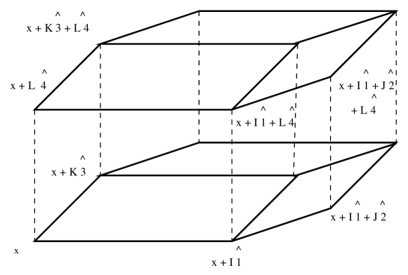
Figure 12: Schematic view of a configuration of the case (I) for the two-point correlator $\langle{\cal W}_{x}(I,J,K){\cal W}_{x+L\hat{4}}(I,J,K)^{*}\rangle_{C}$. Elementary cubes from the action are contracted to fill the space between ${\cal W}_{x}(I,J,K)$ and ${\cal W}_{x+L\hat{4}}(I,J,K)$ indicated by the dashed lines.

The second possibility is that the elementary cubes first fill up each interior of the two Wilson surfaces and leave holes of the minimal size located at $y$ and $y+L\hat{4}$, respectively, and then they are connected at the holes via a stack of minimal number of elementary cubes ($6L$ cubes). See Fig. 13. The contribution is given by

$$(\mbox{Case (II)})=IJK\,\left(\frac{\widetilde{C}_{\Box\Box\Box}(\beta)}{N^{3}}\right)^{2(IJK+3L-1)}\times N^{2(I+J+K+L-3)}\times\Big{[}1+{\cal O}(\beta^{6})\Big{]},$$ (7.39)

where the overall factor $IJK$ comes from the sum with respect to the location of $y$.

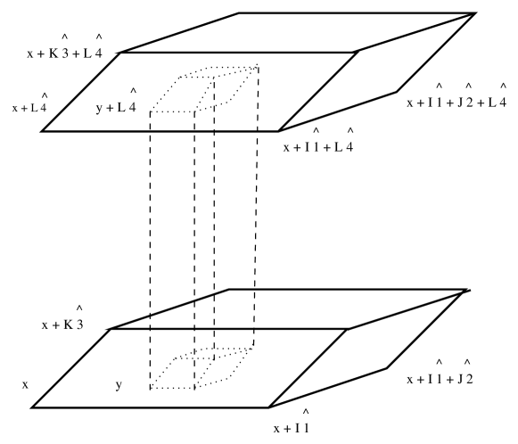
Figure 13: Schematic view of a configuration of the case (II) for the two-point correlator $\langle{\cal W}_{x}(I,J,K){\cal W}_{x+L\hat{4}}(I,J,K)^{*}\rangle_{\rm conn}$. The two surfaces ${\cal W}_{x}(I,J,K)$ and ${\cal W}_{x+L\hat{4}}(I,J,K)$ are connected by the shortest tubular stack of elementary cubes (the dashed lines) attaching at the holes $y$ and $y+L\hat{4}$.

Comparing the power of $\widetilde{C}_{\Box\Box\Box}(\beta)$ for the two cases, we can see which configuration dominates in the strong coupling. For the case $I\sim J\sim K$, the case (II) dominates if $L\mathrel{\mathop{\kern 0.0pt\hbox to0.0pt{\raise 0.86108pt\hbox{$>$}\hss}}\lower 3.87495pt\hbox{\kern-1.90002pt$\sim$}}\frac{1}{6}I$ i.e. the separation is larger than the scale of the surfaces. The case (I) dominates if $L\mathrel{\mathop{\kern 0.0pt\hbox to0.0pt{\raise 0.86108pt\hbox{$<$}\hss}}\lower 3.87495pt\hbox{\kern-1.90002pt$\sim$}}\frac{1}{6}I$. For generic $I,J,K$, we can draw a similar conclusion. From these considerations, we find that the theory develops a mass gap and screening in that the two-point correlator undergoes a ‘phase transition’ as the separation is varied. The situation is rather analogous to the transition taking place for Wilson loop correlators in gauge theory, as depicted in Fig.14.

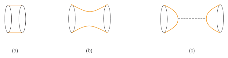
Figure 14: Behavior of the Wilson loop two-point correlator in gauge theory. At small separation (a), the first Wilson loop is joined by a minimal surface to the second Wilson loop. At moderate separation (b), the minimal surface deflects in the middle. At large separation (c), each Wilson loop is filled up by respective minimal surface, joined by a thin tubular column.

7.5 Large-$N$ Reduction and Asymptotic Behavior

In lattice gauge theory, it is well known that large $N$ limit exhibit reduction of degrees of freedom, so-called Eguchi-Kawai reduction. In this section, we will find an indication that a similar reduction takes place in the large $N$ limit of the lattice tensor gauge theory.

To observe an indication, consider again the strong coupling expansion of the partition function Eq.(7.29). There, all the correction terms in the square bracket are suppressed by some power of $1/N$ as the $(\widetilde{C}_{\Box\Box\Box}(\beta))^{8}$ term. Under $N\rightarrow\infty$ limit with $\beta$ fixed, we can discard the correction terms, at least at leading order in $1/N$ expansion. We then see that the partition function ${\cal Z}$ is reduced to the following zero-dimensional, unitary three-matrix model:

$${\cal Z} \Rightarrow \left(Z_{\rm MM}\right)^{\frac{1}{3!}d(d-1)(d-2){\cal N}_{s}}$$ (7.40)

where

$$Z_{\rm MM} = C_{000}(\beta)=\int[{\rm d}U][{\rm d}V][{\rm d}W]\,e^{3\beta\,({\rm tr}\,U)\,({\rm tr}\,V)\,({\rm tr}\,W)+\,{\rm c.c.}}.$$ (7.41)

In this limit, the elementary Wilson surface operator ${\cal W}_{x}(1,1,1)$ alone yields a nonvanishing vacuum expectation value $\widetilde{C}_{\Box\Box\Box}(\beta)$. The connected two-point correlators vanish, and thus the large $N$ factorization

$$\langle{\cal W}_{x}(1,1,1){\cal W}_{x^{\prime}}(1,1,1)\rangle=\langle{\cal W}_{x}(1,1,1)\rangle\,\langle{\cal W}_{x^{\prime}}(1,1,1)\rangle$$ (7.42)

holds.

In the strong coupling expansion, the matrix model partition function $Z_{\rm MM}$ still captures the divergent behavior of perturbation series. As $N\rightarrow\infty$, the $n!$ growth in the series $C_{000}(\beta)$ continues to infinite orders. Therefore, the perturbation series is divergent and not Borel summable. Likewise, for the free energy $\ln Z_{\rm MM}$, the perturbation series behaves asymptotically as $n!\,(3\beta)^{2n}$.

The Borel non-summability of the strong-coupling expansion implies that the entropy in defining the lattice partition function of the tensor gauge theory grows much faster than that of the Yang-Mills theory. Intuitively, we can understand this by the following geometric considerations. At large $N$ limit, the strong coupling expansion of Yang-Mills partition function is interpretable as sum over random surfaces. Likewise, at large $N$ limit, we found above that the strong coupling expansion of nonabelian tensor partition function is interpretable as sum over random volumes. Thus, we would like to compare the entropy of random volumes in comparison with the entropy of random surfaces. So, consider the partition function of random surfaces $\Sigma$ of area $A$. For a fixed area $A$, the partition function takes the form

$$Z(A,\mu,N)=\sum_{\chi}e^{-\mu A}A^{-\chi}N^{-\chi}$$ (7.43)

for a fixed area $A$. The sum is over all possible topologies of the random surface $\Sigma$. We are interested in the density of states, equivalently, density of states. At fixed $N$, it is known that the partition function scales as [34]

$$Z\sim\exp(A\log A).$$ (7.44)

This implies that the entropy $S$ of the random surface for a spherical topology must behave as

$$S(\mathbb{S}^{2})\sim e^{cA}A^{\nu}$$ (7.45)

for some numerical factors $c,\nu$. that the entropy of random volume of $S^{3}$ topology behaves as

$$S(\mathbb{S}^{3})\sim\exp(\alpha A\log A).$$ (7.46)

The proof goes as follows. Consider the map from $\mathbb{R}^{3}$ to itself. The map may be represented by a vector ${\bf X}={\bf X}(\xi^{1},\xi^{2},\xi^{3})$. The map has folds at critical points where

$${\rm det}\left({\partial{\bf X}\over\partial\xi}\right)=0.$$ (7.47)

But, the boundaries of the folds are nothing but 2-dimensional random surfaces. For the latter, we already know that the partition function behaves as Eq.(7.44). Hence, we know that the entropy of random volume ought to behave the same way, viz.

$$Z(\mathbb{S}^{3})\sim\exp(V_{3}\log V_{3}).$$ (7.48)

The reduction implies ultra-local nature of the theory, with no degrees of freedom propagating. In Wilson’s lattice gauge theory case, such a reduction is different from the large $N$ reduction of Eguchi-Kawai [24], and does not lead an interesting theory. In fact, the free energy simply gives $\ln z(\gamma)=\gamma^{2}$ in the limit $N\rightarrow\infty$ with $\gamma$ fixed. In the tensor theory case, however some nontrivial pieces corresponding to singular configurations of three-manifolds seem to remain after the reduction.

Of course, this argument on the large $N$ limit is rather formal. Discarding the correction terms needs to be justified by a careful treatment. About this, we will report elsewhere.

8 Discussions

We constructed a lattice model for a nonabelian generalization of two-form tensor gauge theory starting from an observation of the Wilson’s lattice theory. Requirement of consistent dimensional reduction to lower dimensional Yang-Mills theory uniquely determines the theory, which satisfies compactness conditions of rank-$N^{2}$(I). Also, computation of strong coupling expansion was done for the partition function and some Wilson surface observables. There, the character expansion coefficients much more rapidly grow as a power series of the coupling $\beta$ compared to the ordinary lattice gauge theory case. It possibly suggests that singular contributions to random three-dimensional geometry are much more dominant than those to two-dimensional one.

There are many interesting and important related to this work. We will mention some directly related problems of them.

• The continuum limit at quantum level needs to be understood better. In the classical continuum limit, we found that the tensor gauge theory becomes purely Gaussian. However, there is a possibility that the lattice theory we formulated may have a nontrivial ultraviolet fixed point, where an interacting quantum theory of nonabelian tensor gauge fields can be defined. It would be very interesting to explore the possibility via numerical simulation.

• Universality, which is also related to a suitable continuum limit, need to be understood better. Namely, is the continuum theory independent of the latticization? Here, we constructed the model on a hypercubic lattice, where the plaquette variables $(U_{\mu\nu}(x))_{ijkl}$ encode the square lattice structure (and thus the hypercubic one) to the four color indices $i,j,k,l$. Since the dynamical variables explicitly depend on information of the latticization, at a glance the universality issue seems to be problematic. (In the ordinary lattice gauge theory case, variables are assigned on links. Note that each link variable does not explicitly depend on a lattice structure — triangular lattice, square lattice, and so on.) By solving the rank $N^{2}$(I) conditions, however we can rewrite them as ‘dual’ link variables. Now, the hypercubic structure is not explicitly visible any longer in each ‘dual’ link variable! Thus, the theory with rank $N^{2}$(I) conditions seems hopeful also from the viewpoint of universality. Anyway, check of the universality is an important issue related to the Lorentz invariance of the resulting continuum theory.

• The behavior $n!\,(3\beta)^{2n}$ in the character expansion coefficients reminds us of higher order behavior of weak coupling perturbation series in quantum field theory, rather than the strong coupling. It might suggest an interesting possibility that strong coupling region of the large-$N$ theory is dual to some perturbative field theory.

• We discussed a large $N$ reduction in somewhat speculative way. Related to the duality, it would be interesting to investigate weak coupling phase in the unitary three-matrix model similar to Ref. [25].

  $\bullet$ Supersymmetric extension of the lattice tensor gauge theory is very important, especially, in the context of $(5+1)$-dimensional (2,0) theory. In recent years, there has been enormous progress in formulating supersymmetric Yang-Mills theory on a lattice. In the present context, however, there are further stumbling blocks that need to be overcome. In (2,0) theory, degrees of freedom involves not the whole of tensor gauge field but only self-dual part of it. Self-dual tensor field in (5+1) dimensions is chiral, described by field equations which is first-order in time. Therefore, once put on a lattice naively, the self-dual tensor field would faces the problem of species doubling — the tensor field on the lattice would involve not only self-dual part but also anti-self-dual part. The situation is exactly the same as chiral bosons and chiral fermions in (1+1) dimensions.

Appendix

Appendix A Reduction of plaquette variables to link variables

In this appendix, we show that the nonabelian tensor gauge theory proposed in this paper is reduced consistently to Wilson’s lattice gauge theory by truncating internal degrees of freedom, which transform as adjoint representation of $V_{\mu}(x)$, according to the standard dimensional reduction Eq.(3.17).

Under the dimensional reduction, the action density of an elementary cube along $d$-th direction is reduced to that of an elementary plaquette:

$${\cal U}[C_{\mu\nu d}(x)] \Rightarrow N^{2}\,{\cal U}[P_{\mu\nu}(x)],$$

$${\cal U}[P_{\mu\nu}(x)] \equiv {\rm tr}\,\left(U_{\mu}(x)U_{\nu}(x+\mu)U_{\mu}(x+\hat{\nu})^{\dagger}U_{\nu}(x)^{\dagger}\right),$$

where we have used the unitarity relation

$$\sum_{i,j,k,l}\Big{(}U_{\mu\nu}(x)\Big{)}_{ijkl}\Big{(}U_{\mu\nu}(x)\Big{)}_{ijkl}^{*}=N^{2}.$$

Both of ${\cal U}[C_{\mu dd}(x)]$ and ${\cal U}[C_{ddd}(x)]$ reduce to $N^{3}$, but do not contribute to the action.

Thus, after the lattice dimensional reduction, the action becomes

$$S_{\rm reduced}=-3\beta N^{2}\sum_{\{x\}}\sum_{\mu,\,\nu=1}^{d-1}{}^{\prime}\hskip 5.69054pt\mbox{Re}\,\Big{(}{\cal U}[P_{\mu\nu}(x)]-N\Big{)}-\beta\sum_{\{x\}}\sum_{\mu,\,\nu,\,\lambda=1}^{d-1}\,\mbox{Re}\,\Big{(}{\cal U}[C_{\mu\nu\lambda}(x)]-N^{3}\Big{)}.$$

Here the prime (^′) refers to sum over $\mu,\nu$ omitting $\mu=\nu$ terms, viz. ${\cal U}[P_{\mu\mu}(x)]=N$ contribution. Evidently, the resulting action describes Wilson’s lattice gauge theory together with the nonabelian lattice tensor gauge theory, both in $(d-1)$ dimensions.

As shown in section 3, in the classical continuum limit, the second term in the reduced action scales as ${\cal O}(a^{6})$. On the other hand, expanding the link variable $U_{\mu}(x)=e^{iaA_{\mu}(x)}$, the first term produces the Yang-Mills action at ${\cal O}(a^{4})$. Thus, in the classical continuum limit, the first term dominates over the second, and the system is reduced to the ordinary U($N$) gauge theory. This conclusion is valid for theories defined by both rank-$N^{2}$(I) and rank-$N$ compactness conditions.

Appendix B Alternative nonabelian tensor gauge theory

In this Appendix, we shall consider alternative proposal for the nonabelian tensor gauge theory and study its properties. The alternative one is defined in terms of the rank-$N$ Eqs.(3.13 – 3.16). We shall construct the theory explicitly, work out classical continuum limit and dimensional reduction thereof, and demonstrate that this alternative theory does not lead to a physically meaningful theory.

B.1 polar parametrization of plaquette variable

We will first develop an explicit parametrization of the plaquette variables that solves the compactness conditions Eqs.(3.13 – 3.16).

We find it convenient to introduce a set $M$ of $(N^{2}\times N^{2})$ matrices, and treat the plaquette variable $\left(U_{\mu\nu}(x)\right)_{ijkl}$ as an element of $M$ where $(i,j)$ and $(k,l)$ are interpreted as column and row indices. For general elements $A_{ijkl}$ and $B_{ijkl}$ in $M$, we define a matrix multiplication by $(AB)_{ijkl}=\sum_{m,n}A_{ijmn}B_{mnkl}$. Evidently, $I_{ijkl}=\delta_{ik}\delta_{jl}$ is an identity element of the product. We define trace of matrices as ${\rm Tr}\,A\equiv\sum_{ij}A_{ijij}.$ We also introduce a ‘twist’ matrix $C_{ijkl}\equiv\delta_{il}\delta_{jk}$ acting on a matrix $A_{ijkl}$ as

$$(CA)_{ijkl}=A_{jikl},\quad(AC)_{ijkl}=A_{ijlk}.$$

Using these notations, the condition Eq.(3.5) is written as

$$CU_{\mu\nu}(x)^{\dagger}C=U_{\nu\mu}(x),$$ (B.1)

where the ‘$\dagger$’ refers to hermitian conjugation for the $N^{2}\times N^{2}$ matrices.

In the $(N^{2}\times N^{2})$ matrix representation, the compactness conditions Eq.(3.13 – 3.16) are expressible as

$$\sum_{k}\Big{(}U_{\mu\nu}(x)U_{\mu\nu}(x)^{\dagger}\Big{)}_{iki^{\prime}k} = N\delta_{ii^{\prime}},$$ (B.2)

$$\sum_{k}\Big{(}U_{\mu\nu}(x)U_{\mu\nu}(x)^{\dagger}\Big{)}_{kjkj^{\prime}} = N\delta_{jj^{\prime}},$$ (B.3)

$$\sum_{k}\Big{(}U_{\mu\nu}(x)^{\dagger}U_{\mu\nu}(x)\Big{)}_{iki^{\prime}k} = N\delta_{ii^{\prime}},$$ (B.4)

$$\sum_{k}\Big{(}U_{\mu\nu}(x)^{\dagger}U_{\mu\nu}(x)\Big{)}_{kjkj^{\prime}} = N\delta_{jj^{\prime}}.$$ (B.5)

Since $U_{\mu\nu}(x)$ is a matrix over $\mathbb{C}$, we parametrize it via (a symmetric version of) the polar decomposition:

$$U_{\mu\nu}(x)=e^{\frac{i}{2}a^{2}H_{\mu\nu}(x)}\,R_{\mu\nu}(x)\,e^{\frac{i}{2}a^{2}H_{\mu\nu}(x)}$$

for every $\mu,\nu$, where $a$ is a lattice spacing, and $H_{\mu\nu}(x)$ is a $(N^{2}\times N^{2})$ Hermitian matrix parametrizing the U($N^{2}$) subset of the configuration space ${\mathbb{X}}_{N}$. $R_{\mu\nu}(x)$ is a positive semi-definite $(N^{2}\times N^{2})$ Hermitian matrices. The condition Eq.(3.5) implies that

$$CH_{\mu\nu}(x)C=-H_{\nu\mu}(x),\qquad CR_{\mu\nu}(x)C=R_{\nu\mu}(x).$$

Also, the compactness conditions Eq.(B.2 – B.5) read

$$\sum_{k}\Big{(}e^{\frac{i}{2}a^{2}H_{\mu\nu}(x)}R_{\mu\nu}(x)^{2}e^{-\frac{i}{2}a^{2}H_{\mu\nu}(x)}\Big{)}_{ikjk}=\sum_{k}\Big{(}e^{\frac{i}{2}a^{2}H_{\mu\nu}(x)}R_{\mu\nu}(x)^{2}e^{-\frac{i}{2}a^{2}H_{\mu\nu}(x)}\Big{)}_{kikj}=N\delta_{ij}.$$ (B.6)

In the polar parametrization adopted above, the field $R_{\mu\nu}(x)$ is expandable around the identity $I$ as

$$R_{\mu\nu}(x)^{2}=I-2a^{2}A_{\mu\nu}(x)+a^{4}c_{2}A_{\mu\nu}(x)^{2}+a^{6}c_{3}A_{\mu\nu}(x)^{3}+\cdots.$$ (B.7)

Here, $A_{\mu\nu}(x)$ are $(N^{2}\times N^{2})$ Hermitian matrices, and $c_{2},c_{3},\cdots$ are real-valued constants. Taking the trace of Eq.(B.6), we have

$${\rm Tr}\left[R_{\mu\nu}(x)^{2}\right]=N^{2}.$$

At order ${\cal O}(a^{2m})$ ($m$: even), it leads

$$c_{m}{\rm Tr}\left[A_{\mu\nu}(x)^{m}\right]=0,$$

and implies that $A_{\mu\nu}(x)=0$ when $c_{m}\neq 0$. Thus, for $A_{\mu\nu}(x)$ to be nontrivial, we will need to set $c_{m}=0$ for $m$ even.

The coefficients $c_{3},c_{5},\cdots$ are not fixable by the conditions Eq.(B.6) alone. Here, we will consider the simplest case $c_{3}=c_{5}=\cdots=0$ and discuss the classical continuum limit in the next subsection. As will be shown there, the final form of the continuum action does not change even when $c_{3},c_{5},\cdots$ are kept nonzero. Thus, the parametrization of $U_{\mu\nu}(x)$ is given by

$$U_{\mu\nu}(x)=e^{\frac{i}{2}a^{2}H_{\mu\nu}(x)}\,\sqrt{I-2a^{2}A_{\mu\nu}(x)}\,e^{\frac{i}{2}a^{2}H_{\mu\nu}(x)},$$ (B.8)

with $(N^{2}\times N^{2})$ Hermitian matrices $H_{\mu\nu}(x)$, $A_{\mu\nu}(x)$ satisfying the constraints

$$\sum_{k}\left(A_{\mu\nu}(x)\right)_{ikjk}=\sum_{k}\left(A_{\mu\nu}(x)\right)_{kikj}=0,$$ (B.9)

$$\sum_{k}\Big{(}\underbrace{[H_{\mu\nu}(x),\cdots,[H_{\mu\nu}(x)}_{n},A_{\mu\nu}(x)]\cdots]\Big{)}_{ikjk}$$

(B.10)

$$=\sum_{k}\Big{(}\underbrace{[H_{\mu\nu}(x),\cdots,[H_{\mu\nu}(x)}_{n},A_{\mu\nu}(x)]\cdots]\Big{)}_{kikj}=0\quad\mbox{for }n>0,$$ (B.11)

as well as

$$CH_{\mu\nu}(x)C=-H_{\nu\mu}(x)\qquad\mbox{and}\qquad CA_{\mu\nu}(x)C=A_{\nu\mu}(x).$$ (B.12)

Due to the constraints, in general, $A_{\mu\nu}(x)$ cannot move independently of $H_{\mu\nu}(x)$.

B.2 classical continuum limit

The plaquette variable $U_{\mu\nu}(x)$ in Eq.(B.8) is expanded around the identity $I$ as

$$U_{\mu\nu}(x)=I +a^{2}\Big{[}iH_{\mu\nu}(x)-A_{\mu\nu}(x)\Big{]}$$ (B.17)

$$+a^{4}\left[-\frac{1}{2}H_{\mu\nu}(x)^{2}-\frac{1}{2}A_{\mu\nu}(x)^{2}-\frac{i}{2}\left(H_{\mu\nu}(x)A_{\mu\nu}(x)+A_{\mu\nu}(x)H_{\mu\nu}(x)\right)\right]$$

$$+a^{6}\left[-\frac{i}{6}H_{\mu\nu}(x)^{3}-\frac{1}{2}A_{\mu\nu}(x)^{3}-\frac{i}{4}\left(H_{\mu\nu}(x)A_{\mu\nu}(x)^{2}+A_{\mu\nu}(x)^{2}H_{\mu\nu}(x)\right)\right.$$

$$\hskip 28.45274pt\left.+\frac{1}{8}\left(H_{\mu\nu}(x)^{2}A_{\mu\nu}(x)+A_{\mu\nu}(x)H_{\mu\nu}(x)^{2}+2H_{\mu\nu}(x)A_{\mu\nu}(x)H_{\mu\nu}(x)\right)\right]$$

$$+{\cal O}(a^{8}).$$

From the gauge transformation rule Eq.(3.6) and the gauge function expanded as in Eq.(5.20), we obtain infinitesimal gauge transformation rules for $H_{\mu\nu}(x)$ and $A_{\mu\nu}(x)$

$$\Big{(}H_{\mu\nu}(x)\Big{)}_{ijkl} \rightarrow \Big{(}H_{\mu\nu}(x)\Big{)}_{ijkl}+\delta_{ik}\Big{(}\partial_{\mu}\Lambda_{\nu}(x)\Big{)}_{jl}-\delta_{jl}\Big{(}\partial_{\nu}\Lambda_{\mu}(x)\Big{)}_{ik},$$

$$\Big{(}A_{\mu\nu}(x)\Big{)}_{ijkl} \rightarrow \Big{(}A_{\mu\nu}(x)\Big{)}_{ijkl},$$

and observe that $A_{\mu\nu}(x)$ is gauge invariant. Again, as for the theory considered in the text, nonabelian interactions at finite lattice spacing disappears in the classical continuum limit and the gauge transformation rules are reduced to abelian ones. So, in the continuum limit, gauge invariant field strength is

$$\Big{(}{\cal H}_{\mu\nu\lambda}(x)\Big{)}_{ijki^{\prime}j^{\prime}k^{\prime}}\equiv\Big{(}\partial_{\lambda}H_{\mu\nu}(x)\Big{)}_{iji^{\prime}j^{\prime}}\delta_{kk^{\prime}}+\Big{(}\partial_{\mu}H_{\nu\lambda}(x)\Big{)}_{jkj^{\prime}k^{\prime}}\delta_{ii^{\prime}}+\Big{(}\partial_{\nu}H_{\lambda\mu}(x)\Big{)}_{kik^{\prime}i^{\prime}}\delta_{jj^{\prime}},$$

with the same symmetry property of indices as Eq.(5.17).

Substituting the expansion Eq.(B.17) into Eq.(3.1), after some algebra, we arrive at the continuum action

$$S_{\rm tensor} = \frac{1}{2}\beta a^{6}\sum_{\{x\}}\sum_{\mu,\nu,\lambda=1}^{d}\Big{\{}{\rm Tr}_{N^{3}}\left[{\cal H}_{\mu\nu\lambda}(x){\cal H}_{\mu\nu\lambda}(x)\right]+3N\,{\rm Tr}\left[\left(\partial_{\lambda}A_{\mu\nu}(x)\right)^{2}\right]$$ (B.20)

$$\hskip 65.44142pt\frac{}{}+16\,T\left[A_{\mu\nu}(x),A_{\nu\lambda}(x),A_{\lambda\mu}(x)\right]\Big{\}}\,+{\cal O}(a^{7}).$$

Here, ‘${\rm Tr}_{N^{3}}$’ refers to the trace for $(N^{3}\times N^{3})$ matrices, which is defined for a generic element ${\cal A}_{ijki^{\prime}j^{\prime}k^{\prime}}$ as ${\rm Tr}_{N^{3}}({\cal A})\equiv\sum_{i,j,k}{\cal A}_{ijkijk}$. Also, $T\left[A_{\mu\nu}(x),A_{\nu\lambda}(x),A_{\lambda\mu}(x)\right]$ expresses a trilinear interaction term, which is defined for $(N^{2}\times N^{2})$ matrices $X$, $Y$, $Z$ as

$$T[X,Y,Z]\equiv\sum_{i,j,k,l,m,n}\,X_{ijkl}Y_{lmjn}Z_{nkmi}$$ (B.21)

with the cyclic property $T[X,Y,Z]=T[Y,Z,X]=T[Z,X,Y]$. The classical continuum limit is taken as in Eq.(5.16), and the result is Lorentz invariant and gauge invariant.

A remark is in order concerning the remainders in the small lattice spacing expansion. One might wonder if higher-order terms may yield nontrivial contributions. Even if we keep the next order terms and consider

$$a^{6}c_{3}A_{\mu\nu}(x)^{3}+a^{10}c_{5}A_{\mu\nu}(x)^{5}+\cdots$$ (B.22)

in Eq.(B.7), we arrive at the same continuum action. In this case, in solving the conditions Eq.(B.6), Eq.(B.9) remains the same but Eq.(B.11) is replaced by

$$\sum_{k}\Big{(}[H_{\mu\nu}(x),A_{\mu\nu}(x)]\Big{)}_{ikjk}=\sum_{k}\Big{(}[H_{\mu\nu}(x),A_{\mu\nu}(x)]\Big{)}_{kikj}=0,$$ (B.23)

$$\sum_{k}c_{3}\Big{(}A^{3}_{\mu\nu}(x)\Big{)}_{ikjk}=-\frac{1}{4}\sum_{k}\Big{(}[H_{\mu\nu}(x),[H_{\mu\nu}(x),A_{\mu\nu}(x)]]\Big{)}_{ikjk},$$ (B.24)

$$\sum_{k}c_{3}\Big{(}A^{3}_{\mu\nu}(x)\Big{)}_{kikj}=-\frac{1}{4}\sum_{k}\Big{(}[H_{\mu\nu}(x),[H_{\mu\nu}(x),A_{\mu\nu}(x)]]\Big{)}_{kikj},$$ (B.25)

$$\cdots.$$

In the small lattice spacing expansion, only the first term of Eq.(B.22) is relevant, and it leads to $a^{6}{\rm Tr}(c_{3}A_{\mu\nu}(x)^{3})$. Using Eqs.(B.24, B.25), however, the contribution vanishes. Therefore, again, we arrive at the same action as Eq.(B.20).

B.3 lattice dimensional reduction

Following the procedure of section 4.2, we express the dimensionally reduced plaquette variables $U_{d\mu}(x)$, $U_{\mu d}(x)$, $U_{dd}(x)$ in $(N^{2}\times N^{2})$ matrix notation as

$$U_{\mu}(x) \equiv U_{d\mu}(x)=e^{i\frac{a}{2}H_{\mu}(x)}\,\sqrt{I-2aA_{\mu}(x)}\,e^{i\frac{a}{2}H_{\mu}(x)},$$

$$\tilde{U}_{\mu}(x) \equiv U_{\mu d}(x)=e^{i\frac{a}{2}\tilde{H}_{\mu}(x)}\,\sqrt{I-2a\tilde{A}_{\mu}(x)}\,e^{i\frac{a}{2}\tilde{H}_{\mu}(x)},$$

$$U(x) \equiv U_{dd}(x)=e^{i\frac{a}{2}\Phi(x)}\,\sqrt{I-2a\eta(x)}\,e^{i\frac{a}{2}\Phi(x)},$$

where the continuum fields of the mass dimension one are defined as

$$H_{\mu}(x)\equiv rH_{d\mu}(x),\qquad A_{\mu}(x)\equiv rA_{d\mu}(x),$$

(B.28)

$$\tilde{H}_{\mu}(x)\equiv rH_{\mu d}(x),\qquad\tilde{A}_{\mu}(x)\equiv rA_{\mu d}(x),$$

(B.29)

$$\Phi(x)\equiv\frac{r^{2}}{a}H_{dd}(x),\qquad\eta(x)\equiv\frac{r^{2}}{a}A_{dd}(x),$$

satisfying the conditions corresponding to Eqs.(B.9 – B.12):

$$\sum_{k}\left(A_{\mu}(x)\right)_{ikjk}=\sum_{k}\left(A_{\mu}(x)\right)_{kikj}=0,$$

(B.30)

$$\sum_{k}\Big{(}\underbrace{[H_{\mu}(x),\cdots,[H_{\mu}(x)}_{n},A_{\mu}(x)]\cdots]\Big{)}_{ikjk}$$

(B.31)

$$=\sum_{k}\Big{(}\underbrace{[H_{\mu}(x),\cdots,[H_{\mu}(x)}_{n},A_{\mu}(x)]\cdots]\Big{)}_{kikj}=0\quad\mbox{for }n>0,$$

(B.32)

$$CH_{\mu}(x)C=-\tilde{H}_{\mu}(x),\qquad CA_{\mu}(x)C=\tilde{A}_{\mu}(x),$$ (B.33)

$$\sum_{k}\left(\eta(x)\right)_{ikjk}=\sum_{k}\left(\eta(x)\right)_{kikj}=0,$$

(B.34)

$$\sum_{k}\Big{(}\underbrace{[\Phi(x),\cdots,[\Phi(x)}_{n},\eta(x)]\cdots]\Big{)}_{ikjk}$$

(B.35)

$$=\sum_{k}\Big{(}\underbrace{[\eta(x),\cdots,[\eta(x)}_{n},\Phi(x)]\cdots]\Big{)}_{kikj}=0\quad\mbox{for }n>0,$$

(B.36)

$$C\Phi(x)C=-\Phi(x),\qquad C\eta(x)C=\eta(x).$$

The gauge transformation rules are unchanged from Eqs.(6.9 – 6.13). Introducing the $(N\times N)$ matrix notation as

$$\Big{(}H_{\mu}(x)\Big{)}_{ijkl} = \Big{(}h_{\mu}(x)\Big{)}_{ik}\delta_{jl}+\Big{(}H_{\mu}^{(jl)}(x)\Big{)}_{ik},\qquad\sum_{j}H_{\mu}^{(jj)}(x)=0,$$

$$\Big{(}A_{\mu}(x)\Big{)}_{ijkl} = \Big{(}A_{\mu}^{(jl)}(x)\Big{)}_{ik},\qquad\sum_{j}A_{\mu}^{(jj)}(x)={\rm tr}\,A_{\mu}^{(jl)}(x)=0,$$

it turns out that $h_{\mu}$ transforms as a vector gauge field and $H_{\mu}^{(jl)}$, $A_{\mu}^{(jl)}$ as an adjoint matter field:

$$h_{\mu}(x) \rightarrow V(x)\,[h_{\mu}(x)-i\partial_{\mu}]\,V(x)^{\dagger},$$

$$H_{\mu}^{(jl)}(x) \rightarrow V(x)H_{\mu}^{(jl)}(x)V(x)^{\dagger},$$

$$A_{\mu}^{(jl)}(x) \rightarrow V(x)A_{\mu}^{(jl)}(x)V(x)^{\dagger}.$$ (B.40)

Indices in the superscript $(jl)$ do not transform in the continuum limit. Also, both $\Phi$ and $\eta$ transform as (adjoint)$\times$(adjoint):

$$\Big{(}\Phi(x)\Big{)}_{ijkl} \rightarrow \sum_{i^{\prime}j^{\prime}k^{\prime}l^{\prime}}\Big{(}V(x)\Big{)}_{ii^{\prime}}\Big{(}V(x)\Big{)}_{jj^{\prime}}\Big{(}\Phi(x)\Big{)}_{i^{\prime}j^{\prime}k^{\prime}l^{\prime}}\Big{(}V(x)^{\dagger}\Big{)}_{k^{\prime}k}\Big{(}V(x)^{\dagger}\Big{)}_{l^{\prime}l},$$

$$\Big{(}\eta(x)\Big{)}_{ijkl} \rightarrow \sum_{i^{\prime}j^{\prime}k^{\prime}l^{\prime}}\Big{(}V(x)\Big{)}_{ii^{\prime}}\Big{(}V(x)\Big{)}_{jj^{\prime}}\Big{(}\eta(x)\Big{)}_{i^{\prime}j^{\prime}k^{\prime}l^{\prime}}\Big{(}V(x)^{\dagger}\Big{)}_{k^{\prime}k}\Big{(}V(x)^{\dagger}\Big{)}_{l^{\prime}l}.$$ (B.42)

The dimensionally reduced action now reads

$$S = -\beta\sum_{\{x\}}\sum_{\mu,\nu,\lambda=1}^{d-1}\,\mbox{Re}\left[{\cal U}[C_{\mu\nu\lambda}(x)]-N^{3}\right]-3\beta\sum_{\{x\}}\sum_{\mu,\nu=1}^{d-1}\,\mbox{Re}\left[{\cal U}[C_{\mu\nu d}(x)]-N^{3}\right]$$ (B.44)

$$-3\beta\sum_{\{x\}}\sum_{\mu=1}^{d-1}\,\mbox{Re}\left[{\cal U}[C_{\mu dd}(x)]-N^{3}\right]-\beta\sum_{\{x\}}\,\mbox{Re}\left[{\cal U}[C_{ddd}(x)]-N^{3}\right].$$

The first term gives rise to the same contribution as Eq.(B.20) but with the Lorentz indices running over $1,\cdots,d-1$. The second term yields the ${\cal O}(a^{4})$ contribution:

$$-3\beta\sum_{\{x\}}\sum_{\mu,\nu=1}^{d-1}\,\mbox{Re}\left[{\cal U}[C_{\mu\nu d}(x)]-N^{3}\right]$$ (B.49)

$$= \beta a^{4}\sum_{\{x\}}\sum_{\mu,\nu=1}^{d-1}\left\{{\rm tr}\left[\frac{3}{2}N^{2}f_{\mu\nu}(x)^{2}\right.\right.+3N\sum_{k,l}\left(D_{\mu}H^{(kl)}_{\nu}(x)D_{\mu}H^{(lk)}_{\nu}(x)+D_{\mu}A^{(kl)}_{\nu}(x)D_{\mu}A^{(lk)}_{\nu}(x)\right)$$

$$\hskip 28.45274pt-\frac{3}{2}\sum_{i,j,k,l}\left([H_{\mu}^{(ij)}(x),H_{\nu}^{(kl)}(x)][H_{\mu}^{(ji)}(x),H_{\nu}^{(lk)}(x)]+[A_{\mu}^{(ij)}(x),A_{\nu}^{(kl)}(x)][A_{\mu}^{(ji)}(x),A_{\nu}^{(lk)}(x)]\right.$$

$$\hskip 28.45274pt\left.+2[H_{\mu}^{(ij)}(x),A_{\nu}^{(kl)}(x)][H_{\mu}^{(ji)}(x),A_{\nu}^{(lk)}(x)]\right)\left.\frac{}{}\right]$$

$$\hskip 56.9055pt+24\sum_{i,j,k,l}\Big{(}A_{\mu\nu}(x)\Big{)}_{ijkl}{\rm tr}\left(A_{\mu}^{(ki)}(x)A_{\nu}^{(lj)}(x)\right)\left.\frac{}{}\right\}+{\cal O}(a^{5}),$$

where the field strength and the covariant derivatives are defined by

$$f_{\mu\nu} \equiv \partial_{\mu}h_{\nu}-\partial_{\nu}h_{\mu}+i[h_{\mu},h_{\nu}],$$

$$D_{\mu}H_{\nu}^{(ij)} \equiv \partial_{\mu}H_{\nu}^{(ij)}+i[h_{\mu},H_{\nu}^{(ij)}],$$

and similarly for $D_{\mu}A_{\nu}^{(ij)}$.

However, contributions from the third and fourth terms start with the ${\cal O}(a^{3})$ terms as

$$-3\beta\sum_{\{x\}}\sum_{\mu=1}^{d-1}\,\mbox{Re}\left[{\cal U}[C_{\mu dd}(x)]-N^{3}\right]$$ (B.61)

$$= \sum_{\{x\}}\sum_{\mu=1}^{d-1}\Big{(}\left[24\beta a^{3}\eta_{lmjn}(A_{\mu}^{(ik)})_{jl}(A_{\mu}^{(ki)})_{nm}+12\beta a^{4}(\partial_{\mu}\eta_{lmjn})(A_{\mu}^{(ik)})_{jl}(A_{\mu}^{(ki)})_{nm}\right]$$

$$\hskip 42.67912pt+\beta a^{4}\Big{\{}\frac{3}{2}N\,{\rm Tr}\left[(D_{\mu}\Phi)^{2}+(D_{\mu}\eta)^{2}\right]$$

$$\hskip 71.13188pt-6\left[(H_{\mu}^{(ik)})_{nm}(H_{\mu}^{(ki)})_{jl}+(A_{\mu}^{(ik)})_{nm}(A_{\mu}^{(ki)})_{jl}\right]$$

$$\hskip 76.82234pt\times\left[\Phi_{lqun}\Phi_{umjq}+\eta_{lqun}\eta_{umjq}+\Phi_{lqnu}\Phi_{mujq}+\eta_{lqnu}\eta_{mujq}-(\Phi^{2}+\eta^{2})_{lmjn}\right]$$

$$\hskip 71.13188pt+6\left(H_{\mu}^{(ik)}H_{\mu}^{(ki)}+A_{\mu}^{(ik)}A_{\mu}^{(ki)}\right)_{mn}(\Phi^{2}+\eta^{2})_{nqmq}$$

$$\hskip 71.13188pt+3\,{\rm tr}\left(H_{\mu}^{(ik)}H_{\mu}^{(kj)}+A_{\mu}^{(ik)}A_{\mu}^{(kj)}\right){\rm tr}\left(H_{\mu}^{(jl)}H_{\mu}^{(li)}+A_{\mu}^{(jl)}A_{\mu}^{(li)}\right)$$

$$\hskip 71.13188pt-3\,{\rm tr}\left(H_{\mu}^{(ik)}H_{\mu}^{(lj)}+A_{\mu}^{(ik)}A_{\mu}^{(lj)}\right){\rm tr}\left(H_{\mu}^{(ji)}H_{\mu}^{(kl)}+A_{\mu}^{(ji)}A_{\mu}^{(kl)}\right)$$

$$\hskip 71.13188pt-3\,{\rm tr}\left(H_{\mu}^{(ik)}A_{\mu}^{(lj)}-A_{\mu}^{(ik)}H_{\mu}^{(lj)}\right){\rm tr}\left(H_{\mu}^{(ji)}A_{\mu}^{(kl)}-A_{\mu}^{(ji)}H_{\mu}^{(kl)}\right)$$

$$\hskip 71.13188pt+12\left[\Phi_{mlnj}(H_{\mu}^{(qi)})_{nm}+\eta_{mlnj}(A_{\mu}^{(qi)})_{nm}\right]\left([H_{\mu}^{(ik)},H_{\mu}^{(kq)}]+[A_{\mu}^{(ik)},A_{\mu}^{(kq)}]\right)_{jl}\Big{\}}\Big{)}$$

$$+ {\cal O}(a^{5}),$$

and as

$$-\beta\sum_{\{x\}}\,\mbox{Re}\left[{\cal U}[C_{ddd}(x)]-N^{3}\right]$$ (B.68)

$$= 8\beta a^{3}\sum_{\{x\}}T[\eta(x),\eta(x),\eta(x)]$$

$$+ \beta a^{4}\sum_{\{x\}}\left\{\frac{}{}-6\left(\Phi_{nkmi}\Phi_{jilk}+\eta_{nkmi}\eta_{jilk}\right)\right.\left[\Phi_{lqun}\Phi_{umjq}+\eta_{lqun}\eta_{umjq}-(\Phi^{2}+\eta^{2})_{lmjn}\right]$$

$$\hskip 56.9055pt-3\left(\Phi_{nkmi}\Phi_{jilk}+\eta_{nkmi}\eta_{jilk}\right)\left(\Phi_{lqnu}\Phi_{mujq}+\eta_{lqnu}\eta_{mujq}\right)$$

$$\hskip 56.9055pt+3\left(\Phi^{2}+\eta^{2}\right)_{mknk}\left(\Phi^{2}+\eta^{2}\right)_{nqmq}$$

$$\hskip 56.9055pt-\left(\Phi_{imkn}\eta_{lnjm}-\eta_{imkn}\Phi_{lnjm}\right)\left(\Phi_{jpiq}\eta_{kqlp}-\eta_{jpiq}\Phi_{kqlp}\right)\left.\frac{}{}\right\}$$

$$+ {\cal O}(a^{5}),$$

respectively. Here, the covariant derivative for $\Phi$ is defined according to its transformation property as (adjoint)$\times$(adjoint) under U($N$):

$$\left(D_{\mu}\Phi\right)_{ijkl} \equiv \partial_{\mu}\Phi_{ijkl}+i\left(h_{\mu}\right)_{ii^{\prime}}\Phi_{i^{\prime}jkl}+i\left(h_{\mu}\right)_{jj^{\prime}}\Phi_{ij^{\prime}kl}-i\Phi_{ijk^{\prime}l}\left(h_{\mu}\right)_{k^{\prime}k}-i\Phi_{ijkl^{\prime}}\left(h_{\mu}\right)_{l^{\prime}l},\qquad$$ (B.69)

and similarly for $D_{\mu}\eta$. In Eqs.(B.61 – B.69), Einstein convention for Latin indices is assumed for simplicity of the notation.

All the expressions in Eqs.(B.49, B.61, B.68) are manifestly gauge invariant except the first line in the right-hand-side of Eq.(B.61), where $\eta$-field is acted by the ordinary derivative instead of the covariant derivative. To see that it is nevertheless gauge invariant, we will need to consider the ${\cal O}(a)$-correction contributions to the transformation rules Eq.(B.40). One can solve Eq.(6.9) iteratively with respect to $a$ and get

$$h_{\mu}(x) \rightarrow V(x)\left(h_{\mu}(x)-i\partial_{\mu}\right)V(x)^{\dagger}+a\,G_{1}(h_{\mu}(x))+\cdots,$$

$$H_{\mu}^{(jl)} \rightarrow \sum_{j^{\prime},l^{\prime}}\Big{(}V_{\mu}(x)\Big{)}_{jj^{\prime}}\left[V(x)H_{\mu}^{(j^{\prime}l^{\prime})}(x)V(x)^{\dagger}+a\,G_{1}(H_{\mu}^{(j^{\prime}l^{\prime})}(x))\right]\Big{(}V_{\mu}(x)^{\dagger}\Big{)}_{l^{\prime}l}+\cdots,$$

$$A_{\mu}^{(jl)} \rightarrow \sum_{j^{\prime},l^{\prime}}\Big{(}V_{\mu}(x)\Big{)}_{jj^{\prime}}\left[V(x)A_{\mu}^{(j^{\prime}l^{\prime})}(x)V(x)^{\dagger}+a\,G_{1}(A_{\mu}^{(j^{\prime}l^{\prime})}(x))\right]\Big{(}V_{\mu}(x)^{\dagger}\Big{)}_{l^{\prime}l}+\cdots,$$ (B.72)

where the ellipses denote ${\cal O}(a^{2})$-terms and $G_{1}$’s are ${\cal O}(a)$ corrections originating from the $V(x)$-transformations:

$$G_{1}(h_{\mu}(x)) \equiv \frac{1}{2}\Big{[}\left(\partial_{\mu}V(x)\right)h_{\mu}(x)V(x)^{\dagger}+V(x)h_{\mu}(x)\partial_{\mu}V(x)^{\dagger}-i\partial_{\mu}\left(V(x)\partial_{\mu}V(x)^{\dagger}\right)\Big{]},$$

$$G_{1}(H_{\mu}^{(jl)}(x)) \equiv \frac{1}{2}\Big{[}\left(\partial_{\mu}V(x)\right)H_{\mu}^{(jl)}(x)V(x)^{\dagger}+V(x)H_{\mu}^{(jl)}(x)\partial_{\mu}V(x)^{\dagger}\Big{]},$$

$$G_{1}(A_{\mu}^{(jl)}(x)) \equiv \frac{1}{2}\Big{[}\left(\partial_{\mu}V(x)\right)A_{\mu}^{(jl)}(x)V(x)^{\dagger}+V(x)A_{\mu}^{(jl)}(x)\partial_{\mu}V(x)^{\dagger}\Big{]}.$$

For the transformations generated by $V_{\mu}(x)=e^{ia\Lambda_{\mu}(x)}$, Eq.(B.72) is exact and produces no higher order corrections of $a$. The transformation rules of $\Phi$ and $\eta$, Eq.(B.42), are also exact. Under the gauge transformation Eq.(B.72) with the ${\cal O}(a)$-corrections retained, one can check that the first line in the right-hand side of Eq.(B.61) is gauge invariant (up to irrelevant ${\cal O}(a^{5})$-terms).

In the continuum limit, the ${\cal O}(a^{3})$ terms in Eq.(B.61, B.68) dominate over the Yang-Mills contribution Eq.(B.49) of ${\cal O}(a^{4})$. The ${\cal O}(a^{3})$ terms originate from the trilinear coupling of Eq.(B.20). To try to resolve it, if we assumed the mass dimension of $\eta$ being two and rescaled as $\eta\rightarrow a\eta$ in Eqs.(B.61, B.68), the contributions would start from ${\cal O}(a^{4})$ and $\eta_{ijkl}$ would become an auxiliary field imposing the constraint $(A_{\mu}^{(jl)})_{ik}=0$. In this case, however, the theory is not Lorentz invariant because of the quartic interactions of $H_{\mu}^{(jl)}$ that remain in Eq.(B.61). Therefore, the classical continuum limit of the dimensionally reduced action does not yield a physically meaningful theory.

Appendix C ${\cal O}(N^{3})$ solution for rank-$N^{2}$(I) compactness condition

Is it possible to find a solution for the rank-$N^{2}$(I) compactness conditions Eqs.(3.8-3.11), whose degrees of freedom are of order ${\cal O}(N^{3})$ at large $N$? In this appendix, we demonstrate that such a solution can be constructed, and hence demonstrating that Eqs.(3.8-3.11) by themselves are not so restrictive by themselves. What actually renders the dynamical degrees of freedom reduced further to ${\cal O}(N^{2})$ is the orientation condition (3.5). We also demonstrate that, in the naive continuum limit, the gauge degrees of freedom is again reduced to $\left({\rm U}(1)\right)^{N}$.

Two of the compactness conditions, Eqs.(3.8, 3.10), suggests that the plaquete variables are parametrizable as $U_{\mu\nu}(x)=\exp[ia^{2}T_{\mu\nu}(x)]$, where $T_{\mu\nu}(x)$ are $N^{2}\times N^{2}$ hermitian matrix-valued tensor fields. For the moment, for notational simplicity, we shall suppress the indices $\mu,\nu$ and $x$. Then, the hermiticity of the tensor field $T$ is expressed as

$$T_{ijkl}^{*}=T_{klij}.$$ (C.1)

The other two of the compactness conditions, Eqs.(3.9, 3.11), put further constraints, which we shall consider order-by-order in the power-series expansion of the plaquette variables:

$$U_{ijkl}=\delta_{ik}\delta_{jl}+(ia^{2})T_{ijkl}+\frac{1}{2}\left(ia^{2}\right)^{2}\left(T^{2}\right)_{ijkl}+\cdots.$$

Begin with the condition Eq.(3.9). At the order ${\cal O}(a^{2})$, it is satisfied by Eq.(C.1). The order ${\cal O}(a^{4})$ puts the conditions

$$\sum_{k}\Big{[}\,T^{(ik)},T^{(ki^{\prime})}\,\Big{]}=0.$$ (C.2)

Here, each of $T^{(ik)}$ is a $(N\times N)$ matrix-valued tensor field with the notation

$$\left(T^{(ik)}\right)_{jl}\equiv T_{ijkl}.$$

Then the hermiticity condition, Eq.(C.1), is expressed as

$$T^{(ik)\dagger}=T^{(ki)}.$$ (C.3)

At next order, ${\cal O}(a^{6})$, no new constraints arise since Eqs.(C.3, C.2) solve automatically up to this order. At the order ${\cal O}(a^{8})$, we get the constraints:

$$\sum_{m,n,k}\left(T^{(im)}T^{(mn)}T^{(nk)}T^{(ki^{\prime})}-2T^{(ki^{\prime})}T^{(im)}T^{(mn)}T^{(nk)}\right.$$

(C.4)

$$\,\left.-2T^{(mn)}T^{(nk)}T^{(ki^{\prime})}T^{(im)}+3T^{(nk)}T^{(ki^{\prime})}T^{(im)}T^{(mn)}\right)=0.$$ (C.5)

We did not find general solutions for Eq.(C.5). Nevertheless, it is easy to see that the following two cases solve Eq.(C.5) as well as the conditions for the all orders of $a^{2}$:

$$({\rm A}): T^{(ik)}=V\left(\begin{array}[]{ccc}t^{(ik)}_{1}&&\\ &\ddots&\\ &&t^{(ik)}_{N}\end{array}\right)V^{-1}$$ (C.9)

$$({\rm B}): T^{(ik)}=\sum_{m}V_{im}t^{(m)}(V^{-1})_{mk},$$ (C.10)

where in the case (A) $(t^{(ik)}_{n})^{*}=t^{(ki)}_{n}$, and in the case (B) each of $t^{(m)}$ is a $(N\times N)$ hermitian matrix. The case (A) means that $(T^{(ik)})_{jl}$ are simultaneously diagonalizable with respect to the indices $j,l$, while the case (B) requires the diagonalizable structure for the indices $i,k$.

Conditions that arise at higher order ${\cal O}(a^{2K})$ take the form

$$\sum_{p_{1},\cdots,p_{K-1}}T^{(ip_{1})}T^{(p_{1}p_{2})}\cdots T^{(p_{K-1}i^{\prime})}+(-1)^{K}\sum_{q_{1},\cdots,q_{K-1}}T^{(iq_{1})}T^{(q_{1}q_{2})}\cdots T^{(q_{K-1}i^{\prime})}$$

(C.11)

$$+\sum_{\scriptsize{\begin{array}[]{c}n,m\geq 1\\ n+m=K\end{array}}}(-1)^{m}\frac{K!}{n!m!}\sum_{\scriptsize{\begin{array}[]{r}k,q_{1},\cdots,q_{m-1},\\ p_{1},\cdots,p_{n-1}\end{array}}}T^{(kq_{1})}T^{(q_{1}q_{2})}\cdots T^{(q_{m-1}i^{\prime})}T^{(ip_{1})}T^{(p_{1}p_{2})}\cdots T^{(p_{n-1}k)}$$ (C.16)

(C.17)

$$=0.$$ (C.18)

It is a straightforward calculation to see that both of the cases (A) and (B) solve Eq.(C.18). Similarly, it is easy to check that the cases (A) and (B) are solutions for Eq.(3.11) at the same time. Note that in the cases (A) and (B), $t^{(ik)}_{n}$ and $t^{(m)}_{ij}$ have the ${\cal O}(N^{3})$ degrees of freedom respectively. ($V$ has the degrees of freedom of sub-leading order ${\cal O}(N^{2})$.)

The plaquette variables are expressed as

$$U_{\mu\nu}=\exp\left[ia^{2}B_{\mu\nu}\right],\qquad B_{\mu\nu}=\sum_{A}B_{\mu\nu}^{A}T^{A},\qquad B_{\mu\nu}^{A}\in{\bf R},$$

where $T^{A}$ are linearly independent basis taking the form Eq.(C.9) or Eq.(C.10). The orientation condition Eq.(3.5) means

$$-\sum_{A}B_{\mu\nu}^{A}\left(T^{(ki)A}\right)_{lj}=\sum_{A}B_{\nu\mu}^{A}\left(T^{(lj)A}\right)_{ki}.$$

Note that it relates the upper indices $k,i$ to the lower indices $l,j$ for $\left(T^{(ki)A}\right)_{lj}$. For the case (A), it reads

$$-\sum_{A}B_{\mu\nu}^{A}\,\sum_{m}V_{lm}(V^{-1})_{mj}\,t^{(ki)A}_{m}=\sum_{A}B_{\nu\mu}^{A}\,\sum_{m}V_{km}(V^{-1})_{mi}\,t^{(lj)A}_{m}$$

which means the diagonal structure also for the indices $k,i$:

$$t^{(ki)A}_{n}\propto\sum_{m}t_{nm}^{A}V_{km}\left(V^{-1}\right)_{mi}$$

with $t^{A}_{nm}=t^{A}_{mn}$. The degrees of freedom reduce to ${\cal O}(N^{2})$. Similarly, for the case (B), it requires the diagonal structure for the lower indices $l,j$ reducing the degrees of freedom to ${\cal O}(N^{2})$.

Finally, because the gauge transformation rule Eq.(3.6) ought to keep the diagonal structure in the cases (A) and (B), we should consider the gauge group $({\rm U}(1))^{N}$, a subgroup of ${\rm U}(N)$. Thus, the solutions do not lead to an interesting nonabelian tensor theory. Also, since the gauge degrees of freedom do not have enough degrees of freedom to kill the modes of wrong-sign kinetic term (ghosts), the solutions do not seem to lead physically meaningful continuum theory at least in the classical level.

Appendix D Character expansion coefficient $C_{000}(\beta)$

D.1 evaluation of generating function

Here, we compute $C_{000}(\beta)$ we needed in the text for obtaining results for the partition function and the correlators among Wilson surface operator. Using Eq.(7.10), we can express $C_{000}(\beta)$ as

$$C_{000}(\beta)=\sum_{n=0}^{\infty}\frac{(3\beta)^{2n}}{(n!)^{2}}\left[\int[{\rm d}U]\left({\rm tr}\,U{\rm tr}\,U^{\dagger}\right)^{n}\right]^{3}.$$ (D.1)

To compute the U($N$) group integral in the right-hand-side, consider the following generating function:

$$z(\gamma) \equiv \int[{\rm d}U]\,e^{\gamma\,{\rm tr}(U+U^{\dagger})}$$ (D.3)

$$= \sum_{n=0}^{\infty}\frac{\gamma^{2n}}{(n!)^{2}}\,\int[{\rm d}U]\,\left({\rm tr}\,U{\rm tr}\,U^{\dagger}\right)^{n}.$$

The large-$N$ behavior of this integral, with the ’t Hooft coupling $\lambda\equiv N/\gamma$ fixed, was investigated in [25]. Here, we will extend it to finite $N$. Making use of the character expansion:

$$e^{\gamma\,{\rm tr}\,U}=\sum_{\tt R}\,\zeta_{\tt R}(\gamma)\,\chi_{\tt R}(U)\qquad\mbox{and}\qquad e^{\gamma\,{\rm tr}\,U^{\dagger}}=\sum_{\tt R}\,\zeta_{\tt R}(\gamma)\,\chi_{\tt R}(U^{\dagger})$$ (D.4)

and the character orthogonality relations, we find that $z(\gamma)=\sum_{\tt R}\,\zeta_{\tt R}(\gamma)^{2}.$ We shall first evaluate $\zeta_{\tt R}(\gamma)$ by carrying out the integral

$$\zeta_{\tt R}(\gamma)=\int[{\rm d}U]\,\chi_{\tt R}(U^{\dagger})\,e^{\gamma\,{\rm tr}\,U}.$$ (D.5)

Any unitary irreducible representation is labelled by the ordered integers $m_{1}\geq m_{2}\geq\cdots\geq m_{N}$, running over all integer values while keeping the order. Note, however, that the representations that appear in Eq.(D.4) with nonzero $\zeta_{R}(\gamma)$ are restricted to nonnegative $m_{i}$’s, i.e. $m_{1}\geq m_{2}\geq\cdots\geq m_{N}\geq 0$. When $U$ is diagonalized in the form

$$U=\Omega\,\left(\begin{array}[]{ccc}e^{i\phi_{1}}&&\\ &\ddots&\\ &&e^{i\phi_{N}}\end{array}\right)\,\Omega^{\dagger},\qquad\Omega\in{\rm SU}(N)$$ (D.9)

in terms of the shifted weights $h_{i}\equiv N-i+m_{i}$, the character $\chi_{\tt R}(U)$ is expressed as

$$\chi_{\tt R}(U)=\frac{{\rm det}_{j,k}\left(e^{ih_{j}\phi_{k}}\right)}{\Delta(\phi)},$$

where

$$\Delta(\phi)\equiv{\rm det}_{j,k}\left(e^{i(N-j)\phi_{k}}\right)=\prod_{j<k}\left(e^{i\phi_{j}}-e^{i\phi_{k}}\right).$$

Also, the measure becomes

$$[{\rm d}U]=\frac{1}{N!}\,\left(\prod_{i=1}^{N}\frac{{\rm d}\phi_{i}}{2\pi}\right)\,\Delta(\phi)\,\Delta(\phi)^{*}\,{\rm d}\Omega$$

with the normalization for the angular integral as $\int{\rm d}\Omega=1$. Substituting these into Eq.(D.5), after some algebra, we arrive at

$$\zeta_{R}(\gamma)=\prod_{i}\gamma^{m_{i}}\,{\rm det}_{l,j}\frac{1}{(l-j+m_{j})!}=\prod_{i}\gamma^{m_{i}}\,\frac{1}{m_{1}!\cdots m_{N}!}\,\prod_{j<l}\left(1-\frac{m_{l}}{m_{j}+l-j}\right),$$

and hence

$$z(\gamma)=\prod_{m_{1}\geq m_{2}\geq\cdots\geq m_{N}\geq 0}\,\gamma^{2m_{i}}\,\frac{1}{(m_{1}!)^{2}\cdots(m_{N}!)^{2}}\,\prod_{j<l}\left(1-\frac{m_{l}}{m_{j}+l-j}\right)^{2}.$$ (D.14)

D.2 asymptotic behavior

By computing the generating function $z(\gamma)$ explicitly up to ${\cal O}(\gamma^{10})$, we were convinced that it is expressible as

$$z(\gamma)=\sum_{n=0}^{N}\,\frac{\gamma^{2n}}{n!}+\sum_{n=N+1}^{\infty}\,\frac{v_{n}}{n!}\,\gamma^{2n},$$ (D.15)

where $0<v_{n}<1$. In other words, the first $N$ terms coincide with those of $e^{\gamma^{2}}$, but remaining higher terms are suppressed compared to the corresponding terms of $e^{\gamma^{2}}$. At ${\cal O}(\gamma^{2n})$, each term contributing to Eq.(D.14) corresponds to a way of partition of the number $n$ into $N$. For $n\leq N$, the number of such terms is just the number of partition of $n$, but as $n$ goes over $N$ it becomes smaller than the partition number. This is a reason why the suppression factor arises. In fact, the first few terms of $v_{n}$ takes the form:

$$v_{N+1} = 1-\frac{1}{(N+1)!},$$

$$v_{N+2} = 1-\frac{N+1}{(N+2)N!}-\frac{1}{(N+2)!},$$

$$v_{N+3} = 1-\frac{1}{4}\frac{(N+1)(N+2)}{(N+3)N!}-\frac{1}{4}\frac{N(N+3)}{(N+1)(N+2)(N-1)!}-\frac{N+2}{(N+3)(N+1)!}$$

$$-\frac{1}{(N+3)!}.$$

As increasing the order, $v_{n}$ gets smaller. In fact, Eq.(D.15) is consistent with the large-$N$ result for the strong coupling phase studied in [25]

$$\lim_{N\rightarrow\infty}\frac{1}{N^{2}}\ln z(N/\lambda)=\frac{1}{\lambda^{2}}\qquad\mbox{for }\lambda>2.$$

From the power-series Eq.(D.15), we find that

$$\int[{\rm d}U]\,\left({\rm tr}\,U{\rm tr}\,U^{\dagger}\right)^{n}=\left\{\begin{array}[]{cl}n!&\mbox{for }n\leq N\\ v_{n}\,n!&\mbox{for }n\geq N+1,\end{array}\right.$$ (D.23)

and obtain the result

$$C_{000}(\beta)=\sum_{n=0}^{N}\,n!\,(3\beta)^{2n}+\sum_{n=N+1}^{\infty}\,(v_{n})^{3}\,n!\,(3\beta)^{2n}.$$ (D.25)

Due to the cubic power of the $U$-integral term in Eq.(D.1), the expansion coefficient grows as $n!$ up to ${\cal O}(\beta^{2n})$. It is quite different from the ordinary lattice gauge theory case, where the corresponding quantity in $z(\gamma)$ has behavior of $1/n!$.

$N=2$		$N=3$
$n$	$(v_{n})^{3}n!$	$n$	$(v_{n})^{3}n!$	$n$	$(v_{n})^{3}n!$	$n$	$(v_{n})^{3}n!$
$3$	$3.47$	–	—	$21$	$698000$	$39$	$12.4$
$4$	$4.76$	$4$	$21.1$	$22$	$622000$	$40$	$4.20$
$5$	$5.15$	$5$	$75.9$	$23$	$518000$	$41$	$1.37$
$6$	$4.44$	$6$	$224$	$24$	$404000$	$42$	$0.427$
$7$	$3.11$	$7$	$829$	$25$	$296000$	$43$	$0.128$
$8$	$1.80$	$8$	$2410$	$26$	$205000$	$44$	$0.0369$
$9$	$0.872$	$9$	$6380$	$27$	$133000$	$45$	$0.0102$
$10$	$0.360$	$10$	$15300$	$28$	$81500$	$46$	$0.00273$
$11$	$0.128$	$11$	$33400$	$29$	$47300$	$47$	$0.000700$
$12$	$0.0392$	$12$	$66400$	$30$	$26000$	$48$	$0.000173$
$13$	$0.0106$	$13$	$120000$	$31$	$13500$	$49$	$0.0000414$
$14$	$0.00252$	$14$	$199000$	$32$	$6680$	$50$	$9.53\times 10^{-6}$
$15$	$0.000533$	$15$	$302000$	$33$	$3140$
$16$	$0.000101$	$16$	$422000$	$34$	$1400$
$17$	$0.0000172$	$17$	$544000$	$35$	$597$
$18$	$2.66\times 10^{-6}$	$18$	$647000$	$36$	$242$
$19$	$3.73\times 10^{-7}$	$19$	$713000$	$37$	$94.0$
$20$	$4.78\times 10^{-8}$	$20$	$731000$	$38$	$34.9$

Table 1: Numerical values of the coefficients $(v_{n})^{3}n!$ in $C_{000}(\beta)$ (D.25) up to the first 20 and 50 orders for $N=2$ and 3, respectively. We took three significant figures for each value.

D.3 Convergence of $C_{000}(\beta)$

To understand the large-order behavior of the second sum in Eq.(D.25) for finite $N$, we examined the first 20 and 50 terms in the cases $N=2$ and 3, respectively. The result is tabulated in Table 1.

For $N=2$, the value saturates at $n=5$ and then decreases. Suppression rate becomes stronger with increasing order. For $N=3$, the behavior is similar, and saturates at $n=20$. Passing the saturation point, the value decrease rapidly. For both cases, the asymptotic behavior shows clearly that that series converges. However, the convergence should be considered typical only for finite $N$. As $N$ gets larger, the saturation point shifts to a larger $n$ quickly. For infinite $N$, the series is dominated by the first sum, which is neither convergent nor Borel summable.

References

• [1] M. Kalb and P. Ramond, Classical Direct Interstring Action, Phys. Rev. D 9 (1974) 2273.
• [2] J. Polchinski, Dirichlet-Branes and Ramond-Ramond Charges, Phys. Rev. Lett.  75, 4724 (1995) [arXiv:hep-th/9510017].
• [3] O. Alvarez, L.A. Ferreira and J.Sánchez Guillén, A new approach to integrable theories in any dimension, Nucl. Phys. B 529, 689 (1998) [arXiv:hep-th/9710147].
• [4] S. J. Rey, The Higgs Mechanism For Kalb-Ramond Gauge Field, Phys. Rev. D 40, 3396 (1989);
M.A. Levin and X.G. Wen, String net condensation: a physical mechanism for topological phases, Phys. Rev. B 71, 045110 (2005); ibid. Detecting topological order in a ground state wavefunction, Phys. Rev. Lett. 100, 030502 (2008);
H. Bombin and M.A. Martin-Delgado, Exact topological order in D=3 and beyond, Phys. Rev. B 75, 075103 (2007);
L. Fidkowski, M. Freedman, C. Nayak, K. Walker and Z. Wang, From string nets to nonabelions, arXiv:cond-mat/0610583.
• [5] A. Kitaev, Fault-tolerant quantum computation by anyons, Ann. Phys. 303, 2 (2003);
M. Freedman, A. Kitaev, M. Larsen and Z. Wang, Topological quantum computation, Bull. Amer. Math. Soc. (N.S.) 40, 31 (2003);
H. Bombin and M.A. Martin-Delgado, Statistical mechanical models and topological color codes, arXiv:0711.0468;
Y. Zhang, L.H. Kaufmann and M.L. Ge, Universal quantum gate, Yang-Baxterization and Hamiltonian, Int. J. Quant. Inform. 3, 669 (2005).
• [6] P.W. Shor, Schemes for reducing decoherence in quantum memory, Phys. Rev. A 52, 2493 (1995);
A. Calderbank, E. Rains, P.W. Shor and N. Sloane, Quantum error correction and orthogonal geometry, Phys. Rev. Lett. 78, 405 (1997);
J. Preskill, Reliable quantum computers, Proc. R. Soc. London A 454, 385 (1998);
E. Dennis, A. Kitaev, A. Landahl and J. Preskill, Topological quantum memory, J. Math. Phys. 43, 4452 (2002).
• [7] H. G. Ballesteros, L. A. Fernandez, V. Martin-Mayor, A. Munoz Sudupe, G. Parisi and J. J. Ruiz-Lorenzo, The four dimensional site-diluted Ising model: A finite-size scaling study, Nucl. Phys. B 512, 681 (1998) [arXiv:hep-lat/9707017].
• [8] E. Witten, Bound states of strings and p-branes, Nucl. Phys. B 460, 335 (1996) [arXiv:hep-th/9510135].
• [9] E. Witten, Some comments on string dynamics, arXiv:hep-th/9507121; ibid., Five-brane effective action in M-theory, J. Geom. Phys.  22 (1997) 103 [arXiv:hep-th/9610234].
• [10] A. Strominger, Open p-branes, Phys. Lett.  B 383 (1996) 44 [arXiv:hep-th/9512059];
A. Losev, G. W. Moore and S. L. Shatashvili, M & m’s, Nucl. Phys. B 522 (1998) 105 [hep-th/9707250];
O. Aharony, A brief review of ’little string theories’, Class. Quant. Grav.  17 (2000) 929 [hep-th/9911147];
D. Kutasov, Introduction To Little String Theory, Published in ”Trieste 2001, Superstrings and related matters”, pp. 165-209 (World Scientific, Singapore, 2001).
• [11] I. R. Klebanov and A. A. Tseytlin, Entropy of Near-Extremal Black p-branes, Nucl. Phys.  B 475 (1996) 164 [arXiv:hep-th/9604089].
• [12] D. Freed, J. A. Harvey, R. Minasian and G. W. Moore, Gravitational anomaly cancellation for M-theory fivebranes, Adv. Theor. Math. Phys.  2 (1998) 601 [arXiv:hep-th/9803205];
J. A. Harvey, R. Minasian and G. W. Moore, Non-abelian tensor-multiplet anomalies, JHEP 9809 (1998) 004 [arXiv:hep-th/9808060].
• [13] S. S. Gubser, I. R. Klebanov and A. A. Tseytlin, Coupling constant dependence in the thermodynamics of N = 4 supersymmetric Yang-Mills theory, Nucl. Phys.  B 534 (1998) 202 [arXiv:hep-th/9805156];
A. Fotopoulos and T. R. Taylor, Comment on two-loop free energy in N = 4 supersymmetric Yang-Mills theory at finite temperature, Phys. Rev.  D 59 (1999) 061701 [arXiv:hep-th/9811224];
C. J. Kim and S. J. Rey, Thermodynamics of large-N super Yang-Mills theory and AdS/CFT correspondence, Nucl. Phys.  B 564 (2000) 430 [arXiv:hep-th/9905205].
• [14] R. Attal, Combinatorics of nonabelian gerbes with connection and curvature, arXiv:math-ph/0203056;
J.C. Baez, Higher Yang-Mills theory, arXiv:hep-th/0206130;
H. Pfeiffer, Higher gauge theory and a nonabelian genralization of 2-form electrodynamics, arXiv:hep-th/0304074;
J.C. Baez and A.S. Crans, Higher-Dimensional Algebra VI: Lie 2-Algebras, arXiv:math.QA/0307263.;
R. Attal, Homotopy and duality in non-abelian lattice gauge theory, arXiv:hep-th/0308100;
F. Girelli and H. Pfeiffer, Higher gauge theory – differential versus integral formulation, arXiv:hep-th/0309173.
• [15] E. T. Akhmedov, Towards the theory of non-Abelian tensor fields. I, Theor. Math. Phys.  145 (2005) 1646 [Teor. Mat. Fiz.  145 (2005) 321] [arXiv:hep-th/0503234]; ibid. Towards the theory of non-abelian tensor fields. II, Theor. Math. Phys.  147 (2006) 509 [Teor. Mat. Fiz.  147 (2006) 73] [arXiv:hep-th/0506032];
A. Gustavsson, The non-Abelian tensor multiplet in loop space, JHEP 0601 (2006) 165 [arXiv:hep-th/0512341]; ibid. Closed non-abelian strings, Nucl. Phys.  B 814 (2009) 53 [arXiv:0705.3369 [hep-th]].
• [16] K. G. Wilson, Confinement Of Quarks, Phys. Rev. D 10 (1974) 2445.
• [17] J. E. Paton and H. M. Chan, Generalized Veneziano Model With Isospin, Nucl. Phys. B 10 (1969) 516;
N. Marcus and A. Sagnotti, Group theory from ‘quarks’ at the ends of strings, Phys. Lett. B188 (1987) 58.
• [18] E. Witten, Five-brane effective action in M-theory, J. Geom. Phys.  22, 103 (1997) [arXiv:hep-th/9610234] ;
M. Henningson, Phys. Rev. Lett. 85 (2000) 5280; ibid. Commutation relations for surface operators in six-dimensional (2,0) theory, JHEP 0103 (2001) 011;
R. Dijkgraaf, E. Verlinde and M. Vonk, On the partition sum of the NS fivebrane, [arXiv:hep-th/0205281].
• [19] S. J. Rey, The Higgs Mechanism For Kalb-Ramond Gauge Field, Phys. Rev. D 40, 3396 (1989); ibid. The Collective Dynamics And The Correlations Of Wormholes In Quantum Gravity, Nucl. Phys. B 319, 765 (1989); ibid. The Axion Dynamics In Wormhole Background, Phys. Rev. D 39, 3185 (1989).
• [20] S. J. Rey, The Confining Phase Of Superstrings And Axionic Strings, Phys. Rev. D 43, 526 (1991).
• [21] P. Orland, Instantons And Disorder In Antisymmetric Tensor Gauge Fields, Nucl. Phys. B 205 (1982) 107;
R. B. Pearson, Phase Structure Of Antisymmetric Tensor Gauge Fields, Phys. Rev. D 26 (1982) 2013;
T. Onogi and S. Hashimoto, Gauge theory of antisymmetric tensor fields, Phys. Lett. B 266 (1991) 107.
• [22] A. M. Polyakov, Compact Gauge Fields And The Infrared Catastrophe, Phys. Lett. B 59 (1975) 82; ibid. Quark Confinement And Topology Of Gauge Groups, Nucl. Phys. B 120 (1977) 429.
• [23] For example, see J. M. Drouffe and J. B. Zuber, Strong Coupling And Mean Field Methods In Lattice Gauge Theories, Phys. Rept.  102 (1983) 1.
• [24] T. Eguchi and H. Kawai, Reduction Of Dynamical Degrees Of Freedom In The Large N Gauge Theory, Phys. Rev. Lett.  48 (1982) 1063.
• [25] D. J. Gross and E. Witten, Possible Third Order Phase Transition In The Large N Lattice Gauge Theory, Phys. Rev. D 21 (1980) 446;
S. R. Wadia, N = Infinity Phase Transition In A Class Of Exactly Soluble Model Lattice Gauge Theories, Phys. Lett. B 93, 403 (1980).
• [26] Y. Y. Goldschmidt, 1/N Expansion In Two-Dimensional Lattice Gauge Theory, J. Math. Phys.  21 (1980) 1842;
S. Samuel, U(N) Integrals, 1/N and the Dewit-’t Hooft Anomalies, J. Math. Phys.  21 (1980) 2695.
• [27] See, for example, M. Jimbo, Introduction to the Yang-Baxter Equation, in ‘Braid Groups, Knot Theory and Statistical Mechanics’, Eds. C.N. Yang and M.L. Ge (1990, Singapore, World Scientific Co.), and references therein.
• [28] J.L. Gervais and A. Neveu, Novel triangle relation and absence of tachyons in Liouville string field theory, Nucl. Phys. B 238 (1984) 125;
G. Felder, Conformal field theory and integrable systems associated with elliptic curves, in proceedings of the ICM ‘94, arXiv:hep-th/9407154;
P. Etingof and O. Schiffmann, Lectures on the dynamical Yang-Baxter equations, arXiv:math.QA/9908064;
P. Xu, quantum dynamical Yang-Baxter equation over a nonabelian base, arXiv:math.QA/0104071;
P. Etingof, On the dynamical Yang-Baxter equation, arXiv:math.QA/0207008;
L. Feher and I. Marshall, On a Poisson-Lie analogue of the classical Yang-Baxter equation for self-dual Lie algebras, arXiv:math.QA/0208159;
Y. Suris and A. Veselov, Lax Matrices for Yang-Baxter Maps, arXiv:math.QA/0304122;
J. Donin and A. Mudrov, Dynamical Yang-Baxter equation and quantum vector bundles, arXiv:math.QA/0306028;
V.F.R. Jones, In and around the origin of quantum groups, arXiv:math.QA/0309199.
• [29] K. Osterwalder and E. Seiler, Gauge field theories on the lattice, Ann. Phys. (N.Y.) 110 (1978) 440;
E. Seiler, ”Gauge theories as a problem of constructive quantum field theory and statistical mechanics”, Lecture Notes in Physics 159 (Springer, Berlin, 1982).
• [30] T. Eguchi and H. Kawai, Reduction Of Dynamical Degrees Of Freedom In The Large N Gauge Theory, Phys. Rev. Lett.  48, 1063 (1982).
• [31] B. Durhuus, On the structure of gauge invariant classical observables in lattice gauge theories, Lett. Math. Phys. 4 (1980) 515.
• [32] S. Oda and F. Sugino, Gaussian and mean field approximations for reduced Yang-Mills integrals, JHEP 0103, 026 (2001) [arXiv:hep-th/0011175];
F. Sugino, Gaussian and mean field approximations for reduced 4D supersymmetric Yang-Mills integral, JHEP 0107, 014 (2001) [arXiv:hep-th/0105284];
J. Nishimura and F. Sugino, Dynamical generation of four-dimensional space-time in the IIB matrix model, JHEP 0205, 001 (2002) [arXiv:hep-th/0111102];
J. Nishimura, T. Okubo and F. Sugino, Convergent Gaussian expansion method: Demonstration in reduced Yang-Mills integrals, JHEP 0210, 043 (2002) [arXiv:hep-th/0205253].
• [33] N. Arkani-Hamed, A. G. Cohen, D. B. Kaplan, A. Karch and L. Motl, Deconstructing (2,0) and little string theories, JHEP 0301 (2003) 083 [arXiv:hep-th/0110146].
• [34] A. B. Zamolodchikov, On The Entropy Of Random Surfaces, Phys. Lett.  B 117 (1982) 87.