Horizontal visibility graphs: exact results for random time series

Abstract

The visibility algorithm has been recently introduced as a mapping between time series and complex networks. This procedure allows to apply methods of complex network theory for characterizing time series. In this work we present the horizontal visibility algorithm, a geometrically simpler and analytically solvable version of our former algorithm, focusing on the mapping of random series (series of independent identically distributed random variables). After presenting some properties of the algorithm, we present exact results on the topological properties of graphs associated to random series, namely the degree distribution, clustering coefficient, and mean path length. We show that the horizontal visibility algorithm stands as a simple method to discriminate randomness in time series, since any random series maps to a graph with an exponential degree distribution of the shape $P(k)=(1/3)(2/3)^{k-2}$, independently of the probability distribution from which the series was generated. Accordingly, visibility graphs with other $P(k)$ are related to non-random series. Numerical simulations confirm the accuracy of the theorems for finite series. In a second part, we show that the method is able to distinguish chaotic series from i.i.d. theory, studying the following situations: (i) noise-free low-dimensional chaotic series, (ii) low-dimensional noisy chaotic series, even in the presence of large amounts of noise, and (iii) high-dimensional chaotic series (coupled map lattice), without needs for additional techniques such as surrogate data or noise reduction methods. Finally, heuristic arguments are given to explain the topological properties of chaotic series and several sequences which are conjectured to be random are analyzed.

I Introduction

Recently, the visibility algorithm, a new tool for time series analysis, has been introduced visibilidad_pnas . The method, inspired in the concept of visibility visibility , proceeds by mapping time series into graphs according to a specific geometric criterion, in order to make use of complex networks techniques redes2 ; redes3 ; redes4 ; redes5 for characterize time series (some other works based on a similar philosophy can be found in small1 ; small2 ). In short, a visibility graph is obtained from the mapping of a time series into a network according to the following visibility criterion: Two arbitrary data $(t_{a},y_{a})$ and $(t_{b},y_{b})$ in the time series have visibility, and consequently become two nodes in the associated graph, if any other data $(t_{c},y_{c})$ such that $t_{a}<t_{c}<t_{b}$ fulfills

$$y_{c}<y_{a}+(y_{b}-y_{a})\frac{t_{c}-t_{a}}{t_{b}-t_{a}}.$$ (1)

It has been shown visibilidad_pnas that time series structure is inherited in the associated graph, such that periodic, random and fractal series map into motif-like, random exponential and scale-free networks redes1 ; redes2.0 ; redes2.1 , respectively. These findings suggest that the visibility graph may capture the dynamical fingerprints of the process that generated the series. Furthermore, it has been recently pointed out that this algorithm stands as a method for estimating the Hurst exponent $H$ in fractional Brownian series fbm_mandel , since a linear relation between $H$ and the exponent $\gamma$ of the power law degree distribution in the scale free associated visibility graph exists hurst . While being relatively new, some applications of the method to analyze time series, in different contexts from fluid dynamics turbulence or atmospheric sciences hurricanes to finance stock market , have been presented so far.

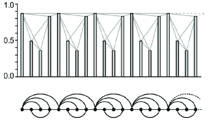
Figure 1: Illustrative example of the visibility algorithm. In the upper part we plot a periodic time series and in the bottom part we represent the graph generated through the visibility algorithm. Each datum in the series corresponds to a node in the graph, such that two nodes are connected if their corresponding data heights fulfill the visibility criterion of equation 1. Note that the degree distribution of the visibility graph is composed by a finite number of peaks, much in the vein of the Discrete Fourier Transform of a periodic signal. We can thus interpret the visibility algorithm as a geometric transform.

What does the visibility algorithm stand for? In order to deepen on the geometric interpretation of the visibility graph, let us focus on a periodic series. It is straightforward that its visibility graph is a concatenation of a motif: a repetition of a pattern (see figure 1). Now, which is the degree distribution $P(k)$ of this visibility graph? Since the graph is just a motif’s repetition, the degree distribution will be formed by a finite number of non-null values, this number being related to the period of the associated periodic series. This behavior reminds us the Discrete Fourier Transform (DFT), which for periodic series is formed by a finite number of peaks (vibration modes) related to the series period. Using this analogy, we can understand the visibility algorithm as a geometric (rather than integral) transform. Whereas a DFT decomposes a signal in a sum of (eventually infinite) modes, the visibility algorithm decomposes a signal in a concatenation of graph’s motifs, and the degree distribution simply makes a histogram of such ’geometric modes’. While the time series is defined in the time domain and the DFT is defined on the frequency domain, the visibility graph is defined on the ’visibility domain’. This is, of course, a hand-waving analogy and further work should study its extent rigorously. For instance, this transform is not, as presented, a reversible one. Reversibility can however be easily obtained weighting the links in the visibility graph with the slope of the visibility line that links the associated data heights. The weighted version of the algorithm and its geometric transform nature will be addressed elsewhere. At this point we can comment that whereas a generic DFT fails to capture the presence of nonlinear correlations in time series (such as the presence of chaotic behavior), in the second part of this paper we will show that the visibility algorithm can clearly distinguish between white noise (i.e. a sequence of identically independent random variables) and chaotic series.
Of course the latter analogy is, so far, a simple metaphor to help our intuition. Indeed, while some analytical results have already been put forward within the visibility algorithm visibilidad_pnas ; hurst (typically making use of concepts borrowed from extreme value theory), no rigorous theory for the visibility algorithms exists so far. Our goal in this work is to make the first steps in that direction, providing results on the properties of the visibility graphs associated to random series. In order to derive exact results, we present here a slight modification of the algorithm that we call the horizontal visibility algorithm, which is essentially similar to the former yet having a geometrically simpler visibility criterion. According to this latter criterion, the generated horizontal visibility graph stands as a subgraph of the visibility graph. We will prove that, surprisingly, the horizontal visibility graph associated to any random series is a Small-World redes2.0 random graph with a universal exponential degree distribution of the form $P(k)=(1/3)\cdot(2/3)^{k-2}$, independently of the probability distribution $f(x)$ from which the series was generated. Accordingly, the horizontal visibility algorithm stands as an extremely simple test for randomness, that for instance, can easily distinguish random series from chaotic ones. The remaining of this paper goes as follows: in section II we introduce the horizontal visibility algorithm, a geometrically simpler version of the visibility algorithm that allows analytical tractability, along with some of its properties. In section III we derive exact results for the degree distribution $P(k)$ of the associated graph to a generic random time series. In section IV exact results on other properties of horizontal visibility graphs are also derived, concretely (i) $P(k|x)$, the probability that a node associated to a datum of height $x$ has degree $k$, (ii) the clustering distribution $P(C)$, (iii) the probability of long distance visibility $P(n)$ and (iv) an estimation of its mean path length $L(N)$ (sections III and IV contain technical proofs that the non-interested reader can eventually skip). In section V we study the reliability of the algorithm to discriminate chaotic series from our theory. For this task we calculate the degree distribution of visibility graphs associated to (i) low-dimensional chaotic series (logistic map, Hénon map), (ii) noisy low-dimensional chaotic series (with amounts of noise of $100\%$ by amplitude), and (iii) high-dimensional chaotic series (coupled map lattice). In every case, the algorithm easily distinguishes those series from a series of i.i.d. random variables (white noise). At this point we also conjecture that the topological properties of graphs associated to chaotic series are related to the statistics of Poincaré recurrence times PRT5 . In section VI we make use of the method as a randomness test, and study some number theoretical sequences that are conjectured to be normal (decimal expansion of normal numbers normal ). We finally provide some concluding remarks in section VII.

II Horizontal visibility algorithm

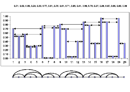
Figure 2: Illustrative example of the horizontal visibility algorithm. In the upper part we plot a time series and in the bottom part we represent the graph generated through the horizontal visibility algorithm. Each datum in the series corresponds to a node in the graph, such that two nodes are connected if their corresponding data heights are larger than all the data heights between them. The data values (heights) are made explicit in the top.

The horizontal visibility algorithm maps time series into graphs and it is defined as follows. Let $\{x_{i}\}_{i=1..N}$ be a time series of $N$ data. The algorithm assigns each datum of the series to a node in the horizontal visibility graph (graph from now on). Two nodes $i$ and $j$ in the graph are connected if one can draw a horizontal line in the time series joining $x_{i}$ and $x_{j}$ that does not intersect any intermediate data height (see figure 2 for a graphical illustration). Hence, $i$ and $j$ are two connected nodes if the following geometrical criterion is fulfilled within the time series:

$$x_{i},x_{j}>x_{n}\ \ \textrm{for all}\ \ n\ \ \textrm{such that}\ \ i<n<j\ .$$ (2)

This algorithm is a simplification of the so called visibility algorithm visibilidad_pnas that has been recently introduced. As a matter of fact, notice that given a time series, its horizontal visibility graph is always a subgraph of its associated visibility graph. Accordingly, as in the former case, the horizontal visibility graph associated to a time series is always:
(i) Connected: each node sees at least its nearest neighbors (left-hand side and right-hand side).
(ii) Invariant under affine transformations of the series data: the visibility criterium is invariant under rescaling of both horizontal and vertical axis, as well as under horizontal and vertical translations.
Some other properties can be stated, namely:
(iii) Reversible/Irreversible character of the mapping: note that some information regarding the time series is inevitably lost in the mapping from the fact that the network structure is completely determined in the (binary) adjacency matrix. For instance, two periodic series with the same period as $T1={...,3,1,3,1,...}$ and $T2={...,3,2,3,2,...}$ would have the same visibility graph, albeit being quantitatively different. Although the spirit of the visibility graph is to focus on time series structural properties (periodicity, fractality, etc.), the method can be trivially generalized by making use of weighted networks (where the adjacency matrix is not binary and the weights determine the height difference of the associated data), if we eventually need to quantitatively distinguish time series like T1 and T2, for instance. Using weighted networks, the algorithm trivially converts to a reversible one.
(iv) Undirected/directed character of the mapping: Although this algorithm generates undirected graphs, note that one could also extract a directed graph (related to the temporal axis direction) in such a way that for a given node one should distinguish two different degrees: an ingoing degree $k_{in}$, related to how many nodes see a given node i, and an outgoing degree $k_{out}$, that is the number nodes that node i sees. In that situation, if the direct visibility graph extracted from a given time series is not invariant under time reversion (that is, if $P(k_{in})\neq P(k_{out}))$, one could assert that the process that generated the series is not conservative. In a first approximation we have studied the undirected version, and the directed one will be eventually addressed in further work. While the undirected choice seems to violate causality, note that the same ’causality violation’ is likely to take place when performing the DFT of a time series, for instance.
(vi) Comparison between geometric criteria: Note that the geometric criterion defined for the horizontal visibility algorithm is more ’visibility restrictive’ than its analogous for the general case. That is to say, the nodes within the horizontal visibility graph will have ’less visibility’ than their counterparts within the visibility graph. While this fact does not have an impact on the qualitative features of the graphs, quantitatively speaking, horizontal visibility graphs will have typically ’less statistics’. For instance, it has been shown that the degree distribution $P(k)$ of the visibility graph associated to a fractal series is a power law $P(k)\sim k^{-\gamma}$, such that the Hurst exponent $H$ of the series is linearly related to $\gamma$ hurst . Now, for practical purposes it is more recommendable to make use of the visibility algorithm (in detriment of the horizontal version) when measuring the Hurst exponent of a fractal series, since a good estimation of $\gamma$ requires at least two decades of statistics in $P(k)$, something which is more likely within the visibility algorithm. In what follows we will show that the simplicity of the horizontal version of the algorithm -which is computationally faster than the original- allows analytical tractability, and nonetheless, this latter method is well fitted to distinguish different degrees of chaos from a sequence of uncorrelated random variables.

III Degree distribution of the visibility graph associated to a random time series

Consider a bi-infinite time series created from a random variable $X$ with probability distribution $f(x)$ with $x\in[0,1]$ and let us construct its associated horizontal visibility graph (note that if the distribution’s support is a generic interval $x\in[a,b]$, we can rescale to $[0,1]$ without loss of generality since the associated graph remains invariant, and this also applies to unbounded supports). For convenience, we will label a generic datum $x_{0}$ as the ‘seed’ datum from now on. In order to derive the degree distribution $P(k)$ redes1 of the associated graph, we need to calculate the probability that an arbitrary datum with value $x_{0}$ has visibility of exactly $k$ other data. If $x_{0}$ has visibility of $k$ data, there always will exist two ‘bounding data’, one on the right-hand side of $x_{0}$ and another one on its left-hand side, such that the $k-2$ remaining visible data will be located inside that window (in fact, $k=2$ is the minimum possible degree). As these ‘inner’ data should appear sorted by size, there are exactly $k-1$ different possible configurations $\{C_{i}\}_{i=0..k-2}$, where the index $i$ determines the number of inner data on the left-hand side of $x_{0}$ (see figure 3 for an illustration of the possible configurations and a labelling recipe of the data in the case $k=4$). Accordingly, $C_{i}$ corresponds to the configuration for which $i$ inner data are placed at the left-hand side of $x_{0}$, and $k-2-i$ inner data are placed at its right-hand side. Each of these possible configurations have an associated probability $p_{i}\equiv p(C_{i})$ that will contribute to $P(k)$ such that

$$P(k)=\sum_{i=0}^{k-2}p_{i}.$$ (3)

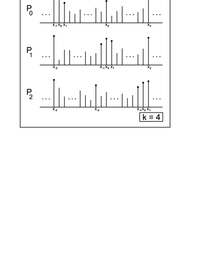
Figure 3: Set of possible configurations for a seed data $x_{0}$ with $k=4$. Observe that the sign of the subindex in $x_{i}$ indicates if the data is located whether at left-hand side of $x_{0}$ (sign minus) or at right-hand side. Accordingly, the bounding’s data subindex directly indicates the amount of data located in that side. For instance, $C_{0}$ is the configuration where none of the $k-2=2$ inner data are located in the left-hand side of $x_{0}$, and therefore the left bounding data is labeled as $x_{-1}$ and the right bounding data is labeled as $x_{3}$. $C_{1}$ is the configuration for which an inner data is located in the left-hand side of $x_{0}$ and another inner data is located in its right-hand side. Finally, $C_{2}$ is the configuration for which both inner data are located in the left-hand side of the seed. Notice that an arbitrary number of hidden data can be eventually located among the inner data, what is schematically represented in the figure as a row of vertical lines.

Before trying to find a general relation for $P(k)$ and for illustrative purposes, let us study some particular cases. The first and simplest case is $P(k=2)$, that is, the probability that the seed data has two and only two visible data, the minimum degree. These obviously will be the bounding data, that we will label $x_{-1}$ and $x_{1}$ for left-hand side and right-hand side of the seed respectively. The probability that $x_{0}$ sees $k\geq 2$ is $1$ by construction, since the horizontal visibility algorithm assures that any data will always have visibility of its first neighbors. Now, in order to assure that $k=2$, we have to impose that the bounding data neighbors have a larger height than the seed, that is, $x_{-1}\geq x_{0}$ and $x_{1}\geq x_{0}$. Then,

$$P(k=2)=\textrm{Prob}(x_{-1},x_{1}\geq 0)=\int_{0}^{1}f(x_{0})dx_{0}\int_{x_{0}}^{1}f(x_{1})dx_{1}\int_{x_{0}}^{1}f(x_{-1})dx_{-1}.$$ (4)

Now, the cumulative probability distribution function $F(x)$ of any probability distribution $f(x)$ is defined as

$$F(x)=\int_{0}^{x}f(x^{\prime})dx^{\prime},$$ (5)

where $dF(x)/dx=f(x)$, $F(0)=0$ and $F(1)=1$. In particular, the following relation between $f$ and $F$ holds:

$$f(x)F^{n-1}(x)=\frac{1}{n}\frac{dF^{n}(x)}{dx}.$$ (6)

We can accordingly rewrite and compute equation 4 as

$$P(k=2)=\int_{0}^{1}f(x_{0})[1-F(x_{0})]^{2}dx_{0}=\frac{1}{3},$$ (7)

independently of the shape of the probability distribution $f(x)$.

Let us proceed by tackling the case $P(k=3)$, that is, the probability that the seed has three and only three visible data. Two different configurations arise: $C_{0}$, in which $x_{0}$ has 2 bounding visible data ($x_{-1}$ and $x_{2}$ respectively) and a right-hand side inner data ($x_{1}$), and the same for $C_{1}$ but with the inner data being place at the left-hand side of the seed, so

$$P(k=3)=p(C_{0})+p(C_{1})\equiv p_{0}+p_{1}.$$

Notice at this point that an arbitrary number $r$ of hidden data $n_{1},n_{2}...n_{r}$ can eventually be located between the inner data and the bounding data, and this fact needs to be taken into account in the probability calculation. The geometrical restrictions for the $n_{j}$ hidden data are $n_{j}<x_{1},\ j=1,...,r$ for $C_{0}$ and $m_{j}<x_{-1},\ j=1,...,s$ for $C_{1}$. Then,

$$p_{0} = \textrm{Prob}\bigg{(}(x_{-1},x_{2}\geq x_{0})\cap(x_{1}<x_{0})\cap(\{n_{j}<x_{1}\}_{j=1,\dots,r})\bigg{)},$$

$$p_{1} = \textrm{Prob}\bigg{(}(x_{-2},x_{1}\geq x_{0})\cap(x_{-1}<x_{0})\cap(\{m_{j}<x_{-1}\}_{j=1,\dots,s})\bigg{)}.$$ (8)

Now, we need to consider every possible hidden data configuration ($C_{0}$ without hidden data, $C_{0}$ with a single hidden data, $C_{0}$ with two hidden data, and so on, and the same for $C_{1}$). With a little calculus we come to

$$p_{0}=\int_{0}^{1}f(x_{0})dx_{0}\int_{x_{0}}^{1}f(x_{-1})dx_{-1}\int_{x_{0}}^{1}f(x_{2})dx_{2}\int_{0}^{x_{0}}f(x_{1})dx_{1}+$$

$$\sum_{r=1}^{\infty}\int_{0}^{1}f(x_{0})dx_{0}\int_{x_{0}}^{1}f(x_{-1})dx_{-1}\int_{x_{0}}^{1}f(x_{2})dx_{2}\int_{0}^{x_{0}}f(x_{1})dx_{1}\prod_{j=1}^{r}\int_{0}^{x_{1}}f(n_{j})dn_{j}$$

where the first term corresponds the contribution of a configuration with no hidden data and the second sums up the contributions of $r$ hidden data. Making use of the properties of the cumulative distribution $F(x)$ we arrive to

$$p_{0}=\int_{0}^{1}f(x_{0})dx_{0}\int_{x_{0}}^{1}f(x_{-1})dx_{-1}\int_{x_{0}}^{1}f(x_{2})dx_{2}\int_{0}^{x_{0}}\frac{f(x_{1})}{1-F(x_{1})}dx_{1},$$ (9)

where we also have made use of the sum of a geometric series. We can find an identical result for $p_{1}$, since the last integral on equation III only depends on $x_{0}$ and consequently the configuration provided by $C_{1}$ is symmetrical to the one provided by $C_{0}$. We finally have

$$P(k=3)=2p_{0}=-2\int_{0}^{1}f(x_{0})(1-F(x_{0}))^{2}\ln(1-F(x_{0}))dx_{0}=\frac{2}{9},$$ (10)

where the last calculation also involves the change of variable $z=1-F(x)$. Again, the result is independent of $f(x)$.

Hitherto, we can deduce that a given configuration $C_{i}$ contributes to $P(k)$ with a product of integrals according to the following rules:

• The seed data provides a contribution of $\int_{0}^{1}f(x_{0})dx_{0}$ (S).

• Each boundary data provides a contribution of $\int_{x_{0}}^{1}f(x)dx$ (B).

• An inner data provides a contribution $\int_{x_{j}}^{x_{0}}\frac{f(x)dx}{1-F(x)}$ (I).

These diagrammatic-like rules allow us to schematize in a formal way the probability associated to each configuration. For instance in the case $k=2$, $P(k)$ has a single contribution $p_{0}$ represented by the formal diagram B-S-B, while for $k=3$, $P(k)=p_{0}+p_{1}$ where $p_{0}$’s diagram is B-S-I-B and $p_{1}$’s is B-I-S-B. It seems quite straightforward to derive a general expression for $P(k)$, just by applying the preceding rules for the contribution of each $C_{i}$. However, there is still a subtle point to address that will become evident for the case $P(k=4)=p_{0}+p_{1}+p_{2}$ (see figure 3). While in this case $C_{1}$ leads to essentially the same expression as for both configurations in $k=3$ (and in this sense one only needs to apply the preceding rules to derive $p_{1}$), $C_{0}$ and $C_{2}$ are geometrically different configurations. These latter ones are configurations formed by a seed, two bounding and two concatenated inner data, and concatenated data lead to concatenated integrals. For instance, applying the same formalism as for $k=3$, one come to the conclusion that for $k=4$,

$$p_{0}=\int_{0}^{1}f(x_{0})dx_{0}\int_{0}^{x_{0}}\frac{f(x_{1})dx_{1}}{1-F(x_{1})}\int_{x_{1}}^{x_{0}}\frac{f(x_{2})dx_{2}}{1-F(x_{2})}\int_{x_{0}}^{1}f(x_{3})dx_{3}\int_{x_{0}}^{1}f(x_{-1})dx_{-1}.$$ (11)

While for the case $k=3$ every integral only depended on $x_{0}$ (and consequently we could integrate independently every term until reaching the dependence on $x_{0}$), having two concatenated inner data on this configuration generates a dependence on the integrals and hence on the probabilities. For this reason, each configuration is not equiprobable in the general case, and thus will not provide the same contribution to the probability $P(k)$ ($k=3$ was an exception for symmetry reasons). In order to weight appropriately the effect of these concatenated contributions, we can make use of the definition of $p_{i}$. Since $P(k)$ is formed by $k-1$ contributions labelled $C_{0},C_{1}...C_{k-2}$ where the index denotes the number of inner data present at the left-hand side of the seed, we deduce that in general the $k-2$ inner data have the following effective contribution to $P(k)$:

• $p_{0}$ has $k-2$ concatenated integrals (right-hand side of the seed).

• $p_{1}$ has $k-3$ concatenated integrals (right-hand side of the seed) and an independent inner data contribution (left-hand side of the seed).

• $p_{2}$ has $k-4$ concatenated integrals (right-hand side of the seed) and another 2 concatenated integrals (left-hand side of the seed).

• …

• $p_{k-2}$ has $k-2$ concatenated integrals (left-hand side of the seed).

Observe that $p_{i}$ is symmetric with respect to the seed.

Including this modification in the diagrammatic rules, we are now ready to calculate a general expression for $P(k)$. Formally,

$$P(k)=\sum_{j=0}^{k-2}[S][B]^{2}[I]_{j}[I]_{k-2-j},$$ (12)

where the sum extends to each of the $k-1$ configurations, the superindex denotes exponentiation and the subindex denotes concatenation (this latter expression can be straightforwardly proved by induction). In order to solve it, one needs to firstly calculate the concatenation of $n$ inner data integrals $[I]_{n}\equiv I(n)$, that is

$$I(n)=\int_{0}^{x_{0}}\frac{f(x_{1})dx_{1}}{1-F(x_{1})}\prod_{j=1}^{n-1}\int_{x_{j}}^{x_{0}}\frac{f(x_{j+1})dx_{j+1}}{1-F(x_{j+1})}.$$ (13)

The calculation of $I(n)$ is easy but quite tedious. One proceeds to integrate equation 13 step by step (first $n=1$, then $n=2$, and so on), and a recurrence quickly becomes evident. One can easily prove by induction that

$$I(n)=\frac{(-1)^{n}}{n!}\bigg{[}\ln\big{(}1-F(x_{0})\big{)}\bigg{]}^{n}.$$ (14)

According to the formal solution 12 and to equation 14, we finally have

$$P(k) = \sum_{j=0}^{k-2}\frac{(-1)^{k-2}}{j!(k-2-j)!}\int_{0}^{1}f(x_{0})[1-F(x_{0})]^{2}[\ln(1-F(x_{0}))]^{k-2}dx_{0}$$ (15)

$$= 3^{1-k}\sum_{j=0}^{k-2}\frac{(k-2)!}{j!(k-2-j)!}=\frac{1}{3}\bigg{(}\frac{2}{3}\bigg{)}^{k-2}$$

Surprisingly, we can conclude that for every probability distribution $f(x)$, the degree distribution $P(k)$ of the associated horizontal visibility graph has the same exponential form.

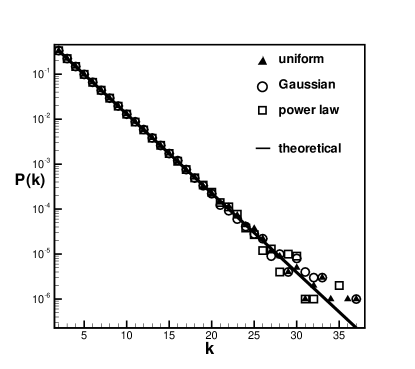
Figure 4: Semi-log plot of the degree distribution of an horizontal visibility graph associated to random series of $10^{6}$ data extracted from a uniform distribution $f(x)=U[0,1]$ (triangles), a Gaussian distribution (circles), and power law distribution $f(x)\sim x^{-2}$ (squares). Solid line corresponds to equation 14.

In order to check further the accuracy of our analytical results for the case of finite time series, we have performed several numerical simulations. We have generated random series of $10^{6}$ data from different distributions $f(x)$ and have generated their associated horizontal visibility graphs. In figure 4 we have plotted the degree distribution of the resulting graphs (triangles correspond to a series extracted from a uniform distribution, while circles and squares correspond to one extracted from a Gaussian and a power law distribution $f(x)\sim x^{-2}$ respectively). The solid line corresponds to the theoretical equation 15, showing a perfect agreement with the numerics.

IV Some other topological properties of the visibility graph

IV.1 Degree versus height

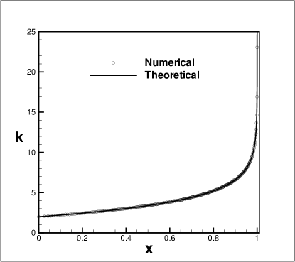
Figure 5: Average degree of a node, as a function of the associated datum’s height: (circles) numeric results from a random series of $10^{6}$ data extracted from a uniform distribution $f(x)=U[0,1]$. The solid line corresponds to the theoretical prediction eq.17, showing a perfect agreement. It comes evident that the hubs stand for the nodes associated to the data with larger values (extreme events).

An interesting aspect worth exploring is the relation between data height and the node degree, that is, to study whether a functional relation between the height of a datum and the degree of its associated node holds. In this sense, let us define $P(k|x)$ as the conditional probability that a given node has degree $k$ provided that it has height $x$. Observe that $P(k|x)$ can be easily deduced from eq. 15, such that

$$P(k|x)=\sum_{j=0}^{k-2}\frac{(-1)^{k-2}}{j!(k-2-j)!}[1-F(x)]^{2}\cdot[\ln(1-F(x))]^{k-2}.$$ (16)

Notice that probabilities are well normalized and that $\sum_{k=2}^{\infty}P(k|x)=1$, independently of $x$. Now, we can define an average value of the degree of a node associated to a datum of height $x$, $K(x)$, in the following way

$$K(x)=\sum_{k-2}^{\infty}kP(k|x)=2-2\ln(1-F(x)).$$ (17)

Since $F(x)\in[0,1]$ and $\ln(x)$ are monotonically increasing functions, $K(x)$ will also be monotonically increasing. We can thus conclude that graph hubs (that is, the most connected nodes) are the data with largest values, that is, the extreme events of the series.
In order to check the accuracy of the theoretical prediction within finite series, in fig. 5 we have plotted (circles) the numerical values of $K(x)$ within a random series of $10^{6}$ data extracted from a uniform distribution with $F(x)=x$. The line corresponds to eq. 17, showing a perfect agreement.

IV.2 Local clustering coefficient distribution

The local clustering coefficient $C$ redes2 ; redes3 ; redes4 ; redes5 ; redes1 of an horizontal visibility graph associated to a random series can be easy deduced by means of geometrical arguments. For a given node $i$, $C$ denotes the rate of nodes connected to $i$ that are connected between each other (observe that in this section, $C$ denotes clustering: do not mistake this with the ’C’ (configuration) of section III). In other words, we have to calculate from a given node $i$ how many nodes from those visible to $i$ have mutual visibility (triangles), normalized with the set of possible triangles ${k\choose 2}$. In a first step, if a generic node $i$ has degree $k=2$, these nodes are straightforwardly two bounding data, hence having mutual visibility. Thus, in this situation there exists $1$ triangle and $C(k=2)=1$. Now if a generic node $i$ has degree $k=3$, one of its neighbors will be an inner data, which will only have visibility of one of the bounding data (by construction). We conclude that in this situation we can only form $2$ triangles out of $6$ possible ones, thereby $C(k=3)=2/6$. In general, for a degree $k$ we can form $k-1$ triangles out of ${k\choose 2}$ possibilities, and then:

$$C(k)=\frac{k-1}{{k\choose 2}}=\frac{2}{k},$$ (18)

what indicates a so called hierarchical structure hierarchical . This relation between $k$ and $C$ allows us to deduce the local clustering coefficient distribution $P(C)$:

$$P(k)=\frac{1}{3}\bigg{(}\frac{2}{3}\bigg{)}^{k-2}=P(2/C)$$

$$P(C)=\frac{1}{3}\bigg{(}\frac{2}{3}\bigg{)}^{2/C-2}$$ (19)

To check the validity of this latter relation within finite series, in figure 6 we depict the clustering distribution of an horizontal visibility graph associated to a random series of $10^{6}$ data (dots) obtained numerically. The solid line corresponds to the theoretical prediction (equation 19), in excellent agreement with the numerics.

Figure 6: Semi-log plot of the clustering distribution of an horizontal visibility graph associated to random series of $10^{6}$ data extracted from a uniform distribution $f(x)=U[0,1]$ (dots). The solid line corresponds to the theoretical prediction $P(C)=(1/3)(2/3)^{2/C-2}$. In order to avoid border effects we have imposed periodic boundary conditions in the data series.

IV.3 Long distance visibility, mean degree and mean path length

In order to derive the scaling of the mean path length redes1 , let us first calculate the probability $P(n)$ that two data separated by $n$ intermediate data be two connected nodes in the graph. Consider again a time series extracted from a random variable $X$ with probability distribution $f(x)$ and $x\in[0,1]$, and let us construct its associated horizontal visibility graph. An arbitrary value $x_{0}$ from this series will ‘see’ $x_{n}$ (and consequently will be connected to node $x_{n}$ in the graph) iff $x_{i}<\min(x_{0},x_{n})$ for all $x_{i},\ i=1,2,...,n-1$. Then $P(n)$ can be expressed as:

$$P(n)=\int_{0}^{1}\int_{0}^{1}f(x_{0})f(x_{n})dx_{0}dx_{n}\int_{0}^{\min(x_{0},x_{n})}\dots$$

$$\dots\int_{0}^{\min(x_{0},x_{n})}f(x_{1})\ldots f(x_{n-1})dx_{1}\dots dx_{n-1}$$ (20)

Since the integration limits are independent, rewriting $x\equiv\min(x_{0},x_{n})$ we have

$$P(n)=\int_{0}^{1}\int_{0}^{1}f(x_{0})f(x_{n})F^{n-1}(x)dx_{0}dx_{n}.$$ (21)

We can fix $x_{0}$ and move $x_{n}$ without loss of generality, such that the latter equation can be expressed as

$$P(n)=\underbrace{\int_{0}^{1}\int_{0}^{x_{0}}f(x_{0})f(x_{n})F^{n-1}(x_{n})dx_{0}dx_{n}}_{\small{\textrm{the minimum here is $x_{n}$}}}+\underbrace{\int_{0}^{1}\int_{x_{0}}^{1}f(x_{0})f(x_{n})F^{n-1}(x_{0})dx_{0}dx_{n}}_{\small{\textrm{the minimum here is $x_{0}$}}}$$ (22)

Applying the definition of $F(x)$ and the relation 6, with a little calculus we get

$$P(n) = \bigg{(}\frac{1}{n}-1\bigg{)}\int_{0}^{1}f(x_{0})F^{n}(x_{0})dx_{0}+\int_{0}^{1}f(x_{0})F^{n-1}(x_{0})dx_{0}$$ (23)

$$= \frac{2}{n(n+1)}.$$

Observe that $P(n)$ is again independent of the probability distribution of the random variable $X$. Notice that the latter result can also be obtained, alternatively, with a purely combinatorial argument that reads as it follows. Take a random series with $n+1$ data and choose its two largest values. This latter pair can be placed with equiprobability in $n(n+1)$ positions, while only two of them are such that the largest values are placed at distance $n$, so we get $P(n)=\frac{2}{n(n+1)}$ on agreement with the previous development.

At this point, we can calculate the mean degree $<k>$ of the horizontal visibility graph:

$$<k>=\sum kP(k)=\sum_{k=2}^{\infty}\frac{k}{3}\Bigg{(}{\frac{2}{3}}\Bigg{)}^{k-2}=4,$$ (24)

that we can recover from $P(n)$ as:

$$<k>=2\sum_{n=1}^{\infty}P(n)=4.$$ (25)

Figure 7: Adjacency matrix of an horizontal visibility graph associated to a random series of $10^{3}$ data.

Now, for illustration purposes, in figure 7 we show the adjacency matrix redes1 of the horizontal visibility graph associated to a random series of $10^{3}$ data (the entry $i,j$ is filled in black if nodes $i$ and $j$ are connected, and left blank otherwise). Since every data $x_{i}$ has visibility of its first neighbors $x_{i-1}$, $x_{i+1}$, every node $i$ will be connected by construction to nodes $i-1$ and $i+1$: the graph is thus connected. Observe in figure 7 that the graph evidences a typical homogeneous structure: the adjacency matrix is predominantly filled around the main diagonal. Furthermore, the matrix evidences a superposed sparse structure, reminiscent of the visibility probability $P(n)=2/(n(n+1))$ that introduces some shortcuts in the horizontal visibility graph, much in the vein of the Small-World model redes2.0 . Here the probability of having these shortcuts is given by $P(n)$. Statistically speaking, we can interpret the graph’s structure as quasi-homogeneous, where the size of the local neighborhood increases with the graph’s size. Accordingly, we can approximate its mean path length $L(N)$ as:

$$L(N)\approx\sum_{n=1}^{N-1}nP(n)=\sum_{n=1}^{N-1}\frac{2}{n+1}=2\log(N)+2(\gamma-1)+O(1/N),$$ (26)

where we have made use of the asymptotic expansion of the harmonic numbers and $\gamma$ is the Euler-Mascheroni constant. As can be seen, the scaling is logarithmic, denoting that the horizontal visibility graph associated to a generic random series is Small-World redes2.0 , according to what figure 6 suggested. In figure 8 we have plotted the numerical results of $L(N)$ (dots) of an horizontal visibility graph associated to several random series of increasing size $N=2^{7},2^{8},\dots 2^{17}$. The solid line corresponds to the best fit $L(N)=1.3\log(N)-1.7$.

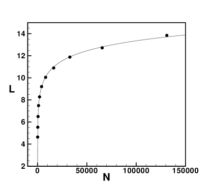
Figure 8: Mean path length $L(N)$ of an horizontal visibility graph associated to random series of $N=2^{7},2^{8},\dots 2^{17}$ data (dots). The solid line corresponds to the better fit $L(N)=1.3\log(N)-1.7$.

V Application of the theory to discriminate chaotic series

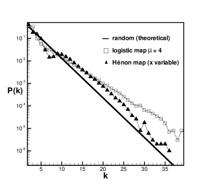
Figure 9: Semi-log plot of the degree distribution of several horizontal visibility graphs associated to: (solid line) theoretical prediction for random series (equation 15), (squares) time series of $10^{6}$ extracted from a logistic map $x_{t+1}=\mu x_{t}(1-x_{t})$ in the fully chaotic region $\mu=4$, (black triangles) time series of $10^{6}$ extracted from $x$ variable of the Hénon map $(x_{t+1},y_{t+1})=(y_{t}+1-ax_{t}^{2},bx_{t})$ in the fully chaotic region ($a=1.4$, $b=0.3$).

So far we have presented exact results on the topological properties of graphs associated to series of i.i.d. random variables (random series from now on) via the horizontal visibility algorithm. The very first application of this theory can be found in the task of discriminating a random signal from a chaotic one. The task of identifying random processes and more concretely discriminating (low dimensional) deterministic chaotic systems from stochastic processes has been extensively studied in the last decades (see for instance procaccia1 ; Farmer ; sugihara ; tsonis ; kaplan ; PRL2007 ; libro_TSA ). Essentially, all methods that have been introduced so far rely on two major points: Firstly, chaotic systems have a finite dimensional attractor, whereas stochastic processes arise from an infinitely dimensional one. Being able to reconstruct this latter attractor is thus a clear evidence showing that the time series has been generated by a deterministic system. Secondly, deterministic systems evidence, as opposed to random ones, short-time prediction: the difference between the time evolution of two nearby states will remain rather low for regular systems and increase exponentially fast for chaotic ones, while for stochastic processes this difference should be randomly distributed. Whereas several algorithms relying on the preceding concepts are nowadays available, the great majority of them are purely numerical and/or usually complicated to perform, computationally speaking (these difficulties are eventually more acute for noisy series noise or high dimensional chaotic ones spatiotemporal ). Furthermore, even the discrimination between a chaotic series and a series of i.i.d. random variables, something that an autocorrelation function or a power spectra fails to do but some other methods such as recurrence plots can kaplan2 is nontrivial when the chaotic degree of the series is high, or even when such series is polluted with noise. All these complications provide motivation for a search for new methods that can directly distinguish, in a reliable way, random from chaotic time series, prior to quantifying the dimension kennel and without needs for additional sophisticated techniques such as surrogate data surrogate or noise reduction methods noise . In the preceding sections we have proved that the horizontal visibility graph associated to a random series has well-defined and universal degree distribution, local clustering distribution and $P(n)$, independent of the shape of the random probability distribution $f(x)$. These theorems guarantee that horizontal visibility graphs with other topological properties are not uncorrelated random series. In what follows we explore the reliability of the method to distinguish uncorrelated randomness from chaos in finite series.

V.1 Low-dimensional chaos

In order to test the practical usefulness of this method, we have generated the horizontal visibility graph of several noise-free chaotic series, and have calculated numerically their degree distribution. We have restricted our analysis to discrete systems (maps), but the method is also extensible to flows (in that case the null hypothesis would no longer be white noise but Brownian motion hurst ). In figure 9 we have plotted in semi-log the results of these simulations. Compare it with figure 3. In every case and by simple visual inspection we can conclude that $P(k)$ deviates from equation 15: the method is able to easily distinguish randomness from low-dimensional chaos (similar results are obtained with $P(n)$ and $P(C)$, but $P(k)$ works better as discriminator).

Observe at this point that if we shuffle the series data and reproduce the analysis, we would find a degree distribution that now would correspond to equation 15, since shuffling breaks the temporal correlations of the series: such shuffled series would be equivalent to a random series extracted from a probability distribution equal to the system’s probability measure (the beta distribution in the case of the Logistic map). We can deduce that the algorithm captures temporal correlations of time series, and that $P(k)$ plays the role of an autocorrelation function, but with the additional ability of capturing nonlinear correlations. Observe also that this method neither works on the time nor on the frequency domain, since it only makes use of topological features.

V.2 Noisy chaotic series

It is well known that standard methods evidence problems when noise is present in chaotic signals, since even a small amount of noise can destroy the fractal structure of a chaotic attractor and mislead the calculation of chaos indicators such as the correlation dimension or the Lyapunov exponents noise . In order to check the algorithm’s robustness, we have introduced an amount of white noise (measurement noise) in a signal extracted from a fully chaotic Logistic map ($\mu=4.0$). In figure 10 we plot the degree distribution of its associated visibility graph. Remarkably, the algorithm still discriminates noisy chaotic behavior from randomness even when the noise level reaches the $100\%$ of the signal amplitude.

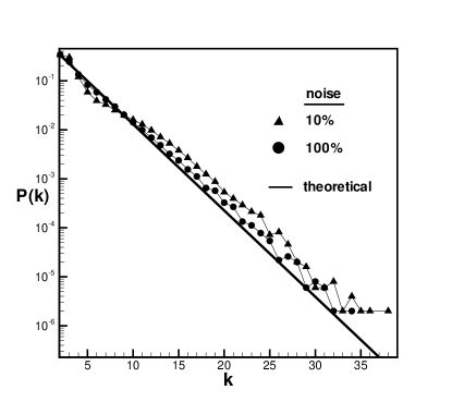
Figure 10: Semi-log plot of the degree distribution of an horizontal visibility graph associated to: (triangles) noisy chaotic series of $10^{5}$ data extracted from the Logistic map ($\mu=4$) with a measurement noise level of $10\%$ (by amplitude), (circles) idem but for noise level of $100\%$. The solid line corresponds to the theoretical prediction for random series $P(k)=(1/3)(2/3)^{k-2}$.

V.3 High dimensional chaos: Coupled Map Lattice

Standard methods of phase space reconstruction also demonstrate computational problems when the attractor dimension is large spatiotemporal . Here we have generated high dimensional chaotic series by means of the so called Coupled Map Lattice (CML) libro_manrubia , a paradigmatic formalism for spatiotemporal chaos, widely used to model chaotic extended systems including fully-developed turbulence and pattern formation problems. We have coupled $N=1000$ Logistic maps $x_{t}^{i},\ i=1,...,N$ such that $x_{t+1}^{i}=f(\epsilon/2x_{t}^{i-1}+(1-\epsilon)x_{t}^{i}+\epsilon/2x_{t}^{i+1})$, where $f(x)=4x(1-x)$ and $\epsilon=0.4$ is the coupling strength (note that such a system exhibits high dimensional chaos with an estimated attractor dimension $D_{2}=800$ spatiotemporal ). In figure 11 we have plotted the degree distribution of its associated visibility graph along with the theoretical prediction for a random series. While the deviations from eq. 15 are not as evident as for low dimensional chaotic series, a $\chi^{2}$ clearly rejects the hypothesis of randomness: the method distinguishes randomness from high dimensional chaos.

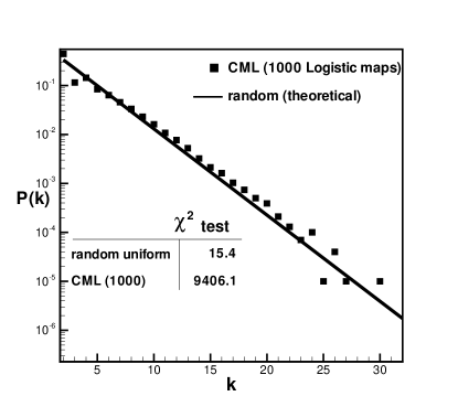
Figure 11: Semi-log plot of the degree distribution of an horizontal visibility graph associated to: (squares) chaotic series of $10^{5}$ data extracted from a CML of 1000 Logistic maps with $\mu=4$ and a coupling strength $\epsilon=0.4$ (see the text). The solid line corresponds to the theoretical prediction for random series $P(k)=(1/3)(2/3)^{k-2}$. Inner box: values of $\chi^{2}$ goodness of fit test between eq. 15 and (i) a random series extracted from a uniform distribution (reference value), (ii) the CML series. While visually speaking the deviations from eq.15 are not here as evident as in the case of low dimensional chaotic series, a $\chi^{2}$ test clearly rejects the hypothesis of randomness (the critical values for $10\%$, $5\%$ and $1\%$ level of significance are 35.2, 38.1 and 41.7 respectively, very far from the value of the test statistic 9406.1): the algorithm distinguishes high-dimensional chaos from randomness.

V.4 Topological properties of chaotic series

Observe in fig. 9 that the series extracted from the Logistic and Hénon maps seem to have an associated visibility graph with a degree distribution which has an exponential tail, yet different to eq. 15. This characteristic can be explained as follows: First, the tail of $P(k)$ is related to the hubs degree. Hubs correspond to the data series that have largest visibility. These are, according to eq. 17, extreme events in the series, whose degree is truncated by other extreme data (statistically speaking). Accordingly, the tail of $P(k)$ essentially reduces to calculate the probability distribution of recurrence times in the series. Within random series, notice that this distribution is straightforwardly exponential (recurrence times in a Poisson process are exponentially distributed Feller ), consistent with eq.15. Within chaotic series, recurrence time statistics are related PRT5 to the concept Poincaré recurrence time (PRT) zaslavsky , which measures the time interval between two consecutive visits of a trajectory to a finite size region of the phase space. As a matter of fact, it has been shown that Poincaré recurrence times are exponentially distributed in several hyperbolic chaotic systems, including the Logistic and Hénon maps (see carleson and references therein). We conjecture that the functional form of $P(k)$ is closely related for chaotic series with their associated Poincaré recurrence time distribution (which deviate from the Poissonian statistics (eq. 15) due to deterministic effects), something that will be addressed in future work.

V.5 Stochastic processes versus chaos

The task of distinguishing determinism from a generic stochastic process (e.g. fractional Brownian motion, high order Markov models, etc) is more general and goes well beyond the scope of this work, since our theory only addresses series of i.i.d. random variables (uncorrelated random series). However, in a recent work hurst it has been shown that fractional Brownian motions and colored noise series map into scale free visibility graphs, which clearly differ from the functional form of $P(k)$ for chaotic series and from i.i.d. theory. In this sense we conjecture that the visibility algorithm efficiently discriminates not only uncorrelated randomness from chaos but also more complicated stochastic processes such as colored noise or fractional Brownian motion.

VI Some conjectured random like series: decimal expansion of normal numbers

A real number $R$ (which can be understood as a series if we pick its decimal expansion) is defined as a normal number if for all integer $k$, any given $k-$tuple is equally likely in the $k-$expansion of $R$; that is to say, the digits of a real number show a uniform distribution in every base normal . For instance, in a decimal base, if number $R$ is normal then every string of size $k$ is equally likely to appear: for $k=4$ the string $3254$ is as likely as $1234$, and this holds for all $k$. It is a well-known result from measure theory that a real number chosen at random is absolutely normal with probability 1. Interestingly, many fundamental constants such as $\pi,e$ or common irrational numbers such as $\ln 2$ or $\sqrt{2}$ are conjectured to be normal, but not a single proof exists so far normal . Now, the degree distribution of a visibility graph associated to the series generated by the decimal expansion of a normal number should follow equation 15. In other words, a deviation from eq. 15 would imply the non-normality of a given number. In table 1 we have reported the values of a $\chi^{2}$ goodness-of-fit test between the degree distribution of graphs associated to the decimal expansion of several conjectured normal numbers (series of $N=100000$ data) and equation 15. The same test has been performed for the case of a random series extracted from a uniform distribution of the same size, for the sake of comparison. As expected, the null hypothesis of normality cannot be rejected. Note that this procedure can easily extend to other number theoretic sequences which are also conjectured to be random.

Series	$\chi^{2}$
Decimal expansion of $\pi$	19.9
Decimal expansion of $e$	20.2
Decimal expansion of $\ln 2$	22.34
Random series extracted from uniform distribution	23.1

Table 1: $\chi^{2}$ goodness-of-fit test between the degree distribution of visibility graphs associated to several number theoretical sequences and the theoretical prediction for random series. The number theoretical sequences are constructed from the decimal expansion of the first $6\cdot 10^{5}$ digits of $\pi,e$ and $\ln 2$, grouped by tuples of 6 elements, what provides series of $10^{5}$ data respectively. As expected, the normality of $\pi,e$ and $\ln 2$ is not rejected by the $\chi^{2}$ test.

VI.1 Note on flows

Notice that the theory that we have developed in sections II to IV addresses a series of i.i.d. variables, that is, a discrete series. Accordingly, we have compared the results obatained from chaotic maps or from the decimal expansion of numbers to this i.i.d. theory, that is, discrete data. Now, it is not straightforward to compare this theory with visibility graphs extracted from flows (continuous series), since in any discretization of a flow some continuity properties are present, something that is not assumed a priori in the i.i.d. theory. This will be addressed in further work.

VII Concluding remarks

In this work we have introduced the horizontal visibility algorithm, an algorithm that maps time series into graphs which is inspired in the so called visibility algorithm visibilidad_pnas . The present algorithm is quite similar to the latter, yet analytically solvable. Accordingly, we have obtained exact results on several properties of the horizontal visibility graph associated to generic uncorrelated random series, and numerical simulations confirmed its reliability for finite series. Concretely, the degree distribution of the graph has an exponential form $P(k)=(1/3)(2/3)^{k-2}$, the clustering coefficient $C$ has a probability distribution $P(C)=(1/3)(2/3)^{2/C-2}$ and the mean path length scales with the system’s size in a logarithmic fashion, evidencing the Small-World phenomenon redes2.0 . Since the results are independent of the distribution from which the series was generated, we conclude that every uncorrelated random series must have the same horizontal visibility graph, and in particular the same degree distribution. Thereby, this algorithm can be used as a simple test for discriminating uncorrelated randomness from chaos. Concretely, we have shown that the method can perfectly distinguish between random series (different probability distributions) that indeed follow the theoretical prediction and chaotic series (logistic map, tent map, Hénon map) that clearly deviate from the theory. This extends to chaotic series polluted with noise and even to high dimensional chaotic series (coupled map lattice).

Observe that this method diverges from the standard algorithms introduced so far libro_TSA since it makes use of graph theoretical techniques to characterize nonlinear temporal correlations of the series, and its recipe is straightforward: (i) construct a visibility graph from the series under study, (ii) compute its degree distribution $P(k)$ and compare it to eq. 15. A visual inspection (or eventually a $\chi^{2}$ goodness-of-fit test between $P(k)$ and equation 15 if needed) allows us to reject the hypothesis that the series is random. The algorithm is direct and has low computational cost, as opposed to several standard methods. Furthermore, it is not just empirical since it is based in exact results. It is worth emphasizing that its purpose is not to quantify chaos but to easily discriminate chaos from uncorrelated randomness. For practical purposes, the method should be used as a reliable preliminary test when looking for deterministic fingerprints in time series (in this sense, once we have checked that $P(k)$ has an exponential tail that deviates from equation 15, embedding methods should be applied to the series). Whether this algorithm is also able to quantify chaos, as well as the relation between standard chaos indicators (Lyapunov exponents, correlation dimension, etc) and the topological properties of the visibility graphs are open problems for further research.
It is also worth commenting that in a preceding work it has been shown that the visibility algorithm is also able to identify colored noise series ($f^{-\beta}$ noises, fractional Brownian motion), since their associated visibility graphs are scale-free hurst , and an algebraic relation between the exponent of the power law degree distribution and the Hurst exponent of the time series exists. In this sense, the visibility algorithm can also discriminate chaos from colored noise.

VIII acknowledgments

The authors acknowledge the interesting comments of two anonymous referees. This work is partially supported by the spanish ministry of science under grant FISXXXXXX.

References

- (1) L. Lacasa, B. Luque, F. Ballesteros, J. Luque and J.C. Nuno, Proc. Natl. Acad. Sci. 105, no. 13 (2008) 4972-4975.
- (2) M. de Berg, M. van Kreveld, M. Overmans and O. Schwarzkopf, in Computational Geometry: Algorithms and Applications, pp. 307-317 (Springer-Verlag, Berlin, 2000).
- (3) R. Albert, A.L. Barabasi, Rev. Mod. Phys. 74 (2002).
- (4) M.E.J. Newman, SIAM Review 45 (2003) 167-256.
- (5) S. Dorogovtsev, J.F.F Mendes, Advances in Physics 51, 4 (2002).
- (6) S. Bocaletti, V. Latora, Y. Moreno, M. Chávez and D.U. Hwang, Phys. Reports 424 (2006) 175-308.
- (7) J. Zhang, M. Small, Phys. Rev. Lett. 96 238701 (2006).
- (8) X. Xu, J. Zhang, M. Small, Proc. Natl. Acad. Sci. USA 105, 50 (2008).
- (9) B. Bollobás, Modern Graph Theory, Springer-Verlag, New York Inc. (1998).
- (10) D.J. Watts and S.H. Strogatz, Nature 393, 440-442 (1998).
- (11) A.L. Barabási, R. Albert, Science 286, 509 (1999).
- (12) B.B Mandelbrot and J.W Van Ness, SIAM Review 10, 4 (1968) 422-437.
- (13) L. Lacasa, B. Luque, J. Luque and J.C. Nuno, EPL 86 (2009) 30001.
- (14) C. Liu, W.X. Zhou, and W.K. Yuan, Arxiv preprint arXiv:0905.1831 (2009).
- (15) E.A. Fogarty, Network Analysis of Hurricanes Affecting the United States, PhD dissertation (2009) etd-03232009-110339.
- (16) Y. Yang, J. Wang, H. Yang, J. Mang, Physica A (2009) (in press).
- (17) E.G. Altmann and H. Kantz, Phys. Rev. E 71, 056106 (2005).
- (18) S. Wagon, The Mathematical Intelligencer 7 (1985) 65-67.
- (19) M. Casdagli, J. R. Statist. Soc. B 54, 2 (1991) pp. 303-328.
- (20) E. Ravasz, A.L. Somera, D.A. Mongru, Z.N. Oltvai, A.-L. Barabasi, Science 297, 1551 (2002).
- (21) P. Grassberger and I. Procaccia, Phys. Rev. Lett. 50, 448 (1983).
- (22) J.D. Farmer and J.J. Sidorovich, Phys. Rev. Lett. 59 (1987) 845-848.
- (23) G. Sugihara and R.M. May, Nature 344, 734 (1990).
- (24) A. A. Tsonis and J. B. Elsner, Nature 358, 217 (1992).
- (25) D.T. Kaplan and L. Glass, Phys. Rev. Lett. 68, 4 (1992).
- (26) O.A. Rosso, H.A. Larrondo, M.T. Martin, A. Plastino, and M.A. Fuentes, Phys. Rev. Lett. 99, 154102 (2007).
- (27) H. Kantz and T. Schreiber, Nonlinear Time Series Analysis, 2nd ed. (Cambridge UNiversity press, Cambridge, 2003).
- (28) E.J. Kostelich and T. Schreiber, Phys. Rev. E 48, 1752 (1993).
- (29) M. Bauer, H. Heng and W. Martienssen, Phys. Rev. Lett. 71, 4 (1993).
- (30) M.B. Kennel and S. Isabelle, Phys. Rev. A 46, 6 (1992).
- (31) D. Prichard and J. Theiler, Phys. Rev. Lett. 73, 7 (1994).
- (32) D. Kaplan and L. Glass, Understanding Nonlinear Dynamics, Springer-Verlag (1996).
- (33) S.C. Manrubia, A.S. Mikhailov, and D.H. Zanette, Emergence of Dynamical Order: Synchronization Phenomena in Complex Systems, World Scientific Publishing Co. (2004).
- (34) W. Feller, An Introduction to Probability Theory and its Applications, John Willey and Sons, Inc. (1971).
- (35) G.M. Zaslavsky, Physics Reports 371 (2002) pp: 461-580.
- (36) M. Benedicks and L. Carleson, Ann. Math. 133 (1991) pp: 73 169, L.-.S. Young, Ann. Math. 147, 3 (1998) pp: 585-650, M. Hirata, B. Saussol, and S. Vaienti, Comm. Math. Phys. 206 (1999) pp: 33-55.