Counting statistics of transport through Coulomb blockade nanostructures:
High-order cumulants and non-Markovian effects

Abstract

Recent experimental progress has made it possible to detect in real-time single electrons tunneling through Coulomb blockade nanostructures, thereby allowing for precise measurements of the statistical distribution of the number of transferred charges, the so-called full counting statistics. These experimental advances call for a solid theoretical platform for equally accurate calculations of distribution functions and their cumulants. Here we develop a general framework for calculating zero-frequency current cumulants of arbitrary orders for transport through nanostructures with strong Coulomb interactions. Our recursive method can treat systems with many states as well as non-Markovian dynamics. We illustrate our approach with three examples of current experimental relevance: bunching transport through a two-level quantum dot, transport through a nano-electromechanical system with dynamical Franck-Condon blockade, and transport through coherently coupled quantum dots embedded in a dissipative environment. We discuss properties of high-order cumulants as well as possible subtleties associated with non-Markovian dynamics.

I Introduction

Electron transport through nanoscale structures is a stochastic process due to the randomness of the individual tunneling events. Quantum correlations and electron-electron interactions can strongly influence the transport process and thus the statistics of transferred charges. Full counting statisticsLevitov and Lesovik (1993); Levitov et al. (1996); Nazarov (2003) concerns the distribution of the number of transferred charge, or equivalently, all corresponding cumulants (irreducible moments) of the distribution. Conventional transport measurements have focused on the first cumulant, the mean current, and in some cases also the second cumulant, the noise.Blanter and Büttiker (2000) Higher order cumulants, however, reveal additional information concerning a variety of physical phenomena, including quantum coherence, entanglement, disorder, and dissipation.Nazarov (2003) For example, non-zero higher-order cumulants reflect non-Gaussian behavior. Counting statistics in mesoscopic physics has been a subject of intensive theoretical interest for almost two decades, but recently it has also gained considerable experimental interest: in a series of experiments,Reulet et al. (2003); Bomze et al. (2005); Bylander et al. (2005); Fujisawa et al. (2006); Gustavsson et al. (2006); Fricke et al. (2007); Timofeev et al. (2007); Gershon et al. (2008); Gabelli and Reulet (2009); Flindt et al. (2009); Gustavsson et al. (2009); Fricke et al. (2010, 2010) high order cumulants and even the entire distribution function of transferred charge have been measured, clearly demonstrating that counting statistics now has become an important concept also in experimental physics.

The theory of counting statistics was first formulated by Levitov and Lesovik for non-interacting electrons using a scattering formalism.Levitov and Lesovik (1993); Levitov et al. (1996) Subsequent works have focused on the inclusion of interaction effects in the theory.Nazarov (1999); Kindermann and Nazarov (2003) In one approach, Coulomb interactions are incorporated via Markovian (generalized) master equations as originally developed by Bagrets and Nazarov.Bagrets and Nazarov (2003) This approach is often convenient when considering systems with strong interactions, e.g., Coulomb-blockade structures. More recent developments include theories for finite-frequency counting statistics,Emary et al. (2007) conditional counting statistics,Sukhorukov et al. (2007) connections to entanglement entropyKlich and Levitov (2009) and to fluctuation theorems,Förster and Büttiker (2008); Esposito et al. (2009) and extensions to systems with non-Markovian dynamics.Braggio et al. (2006); Flindt et al. (2008); Schaller et al. (2009) The last topic forms the central theme of this paper.

We have recently published a series of papers on counting statistics.Flindt et al. (2005a); Braggio et al. (2006); Flindt et al. (2008) Previous methods for evaluating the counting statistics of systems described by master equations had in practice been limited to systems with only a few states, and in Ref. Flindt et al., 2005a we thus developed techniques for calculating the first few cumulants of Markovian systems with many states, for example nano-electromechanical systems.Flindt et al. (2004) In Ref. Braggio et al., 2006, Braggio and co-workers generalized the approach by Bagrets and Nazarov by including non-Markovian effects that may arise for example when the coupling to the electronic leads is not weak. The methods presented in these papers were subsequently unified and extended in Ref. Flindt et al., 2008, where we presented a general approach to calculations of cumulants of arbitrary order for systems with many states as well as with non-Markovian dynamics. The aim of the present paper is to provide a detailed derivation and description of this method, which recently has been used in a number of works,Zedler et al. (2009); Emary (2009); Emary et al. (2009); Urban and König (2009); Lindebaum et al. (2009); Zhong and Cao (2009); Domínguez et al. (2010) as well as to illustrate its use with three examples of current experimental relevance.

The paper is organized as follows: In Sec. II we introduce the generic non-Markovian generalized master equation (GME) which is the starting point of this work. The GME describes the evolution of the reduced density matrix of the system, which has been resolved with respect to the number of transferred particles. Memory effects due to the coupling to the environment as well as initial system-environment correlations are included in the GME. Within this framework it is possible to calculate the finite-frequency current noise for non-Markovian GMEsFlindt et al. (2008) as we will discuss in future works. Section II concludes with details of the superoperator notation used throughout the paper.

In Sec. III we develop a theory for the zero-frequency cumulants of the current. The cumulant generating function (CGF) is determined by a single dominating pole of the resolvent of the memory kernel, and its derivatives with respect to the counting field evaluated at zero counting field yield the cumulants of the current. Even in the Markovian case it is difficult to determine analytically the dominating pole and in many cases one would have to find it numerically. Numerical differentiation, however, is notoriously unstable, and often one can only obtain accurate results for the first few derivatives with respect to the counting field, i. e. the cumulants. In order to circumvent this problem, we develop a numerically stable recursive scheme based on a perturbation expansion in the counting field. The scheme enables calculations of zero-frequency current cumulants of very high orders, also for non-Markovian systems. Some notes on the evaluation of the cumulants are presented, with the more technical numerical details deferred to App. A.

Section IV gives a discussion of the generic behavior of high-order cumulants. As some of us have recently shown,Flindt et al. (2009) the high-order cumulants for basically any system (with or without memory effects) are expected to grow factorially in magnitude with the cumulant order and oscillate as functions of essentially any parameter as well as of the cumulant order. We describe the theory behind this prediction which is subsequently illustrated with examples in Sec. V.

Section V is devoted to two Markovian transport models of current research interest, which we use to illustrate our recursive scheme and the generic behavior of high-order cumulants discussed in Sec. IV. We start with a model of transport through a two-level quantum dot developed by Belzig.Belzig (2005) Due to the relatively simple analytic structure of the model, it is possible to write down a closed-form expression for the CGF, allowing us to develop a thorough understanding of the behavior of high-order cumulants obtained using our recursive scheme. We study the large deviation function of the system,Touchette (2009) which describes the tails of the distribution of measurable currents, and discuss how it is related to the cumulants.

The second example concerns charge transport coupled to quantized mechanical vibrations as considered in a recent series of papers on transport through single moleculesBoese and Schoeller (2001); Braig and Flensberg (2003); McCarthy et al. (2003); Mitra et al. (2004); Koch and von Oppen (2005); Koch et al. (2005); Pistolesi et al. (2008) and other nano-electromechanical systems.Gorelik et al. (1997); Armour and MacKinnon (2002); Fedorets et al. (2002); Novotný et al. (2003, 2004); Flindt et al. (2004); Fedorets et al. (2004); Haupt et al. (2006); Rodrigues et al. (2007); Hübener and Brandes (2007); Harvey et al. (2008); Körting et al. (2009); Hübener and Brandes (2009); Cavaliere et al. (2009); Harvey et al. (2009) Due to the many oscillator states participating in transport the matrix representations of the involved operators are of large dimensions and it is necessary to resort to numerics. We demonstrate the numerical stability of our recursive algorithm up to very high cumulant orders ($\sim 100$) and show how oscillations of the cumulants can be used to extract information about the analytic structure of the cumulant generating function. We calculate the large deviation function and show that it is highly sensitive to the damping of the vibrational mode.

Section VI concerns the counting statistics of non-Markovian systems. We consider a model of non-Markovian electron transport through a Coulomb-blockade double quantum dot embedded in a dissipative heat bath and coupled to electronic leads. The dynamics of the charge populations of the double dot can be described using a non-Markovian GME whose detailed derivation is presented in App. C. We study the behavior of the first three cumulants thus extending previous studies that have been restricted to the noise.Aguado and Brandes (2004a, b) We focus in particular on the influence of decoherenceKießlich et al. (2007) on the charge transport statistics. Finally, we discuss possible subtleties associated with non-Markovian dynamics and we provide the reader with a unifying point of view on a number of results reported in previous studies as well as in the examples discussed in this paper.

Our conclusions are stated in Sec. VII. Appendix A describes the numerical algorithms used to solve the recursive equations for high-order cumulants, while Apps. B and C give detailed derivations of the Markovian GME for the vibrating molecule and the non-Markovian GME for the double-dot system, respectively.

II Generalized Master equation

The generic transport setup under consideration in this work is depicted in Fig. 1: A nanoscopic quantum system is connected by tunneling barriers to two electronic leads, allowing for charge and energy exchange with the leads. Typically, the quantum system consists of a discrete set of (many-body) quantum states. Moreover, the system is coupled to an external heat bath to and from which energy can flow. We will be considering a transport configuration, where a bias difference between the leads drives electrons through the system.

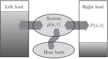
Figure 1: Generic transport setup. A quantum system is connected to electronic leads and a heat bath. A bias difference between the leads drives electrons through the system, which can exchange energy with the surrounding heat bath. The system is described by the $n$-resolved density matrix $\hat{\rho}(n,t)$ (see text), where $n$ is the number of electrons that have been collected in the right lead during the time span $[0,t]$. The probability distribution of $n$ is denoted as $P(n,t)$.

The quantum system is completely described by its (reduced) density matrix $\hat{\rho}(t)$, obtained by tracing out the environmental degrees of freedoms, i. e. the electronic leads and the heat bath. It is, however, advantageous to resolve $\hat{\rho}(t)$ into the components $\hat{\rho}(n,t)$, corresponding to the number of electrons $n$ that have tunneled through the system during the time span $[0,t]$.Makhlin et al. (2001); Shelankov and Rammer (2003); Wabnig et al. (2005) The $n$-resolved density matrix allows us to study the statistics of the number of transferred charges, similarly to well-known techniques from quantum optics.Cook (1981); Lenstra (1982); Plenio and Knight (1998) We note that the (un-resolved) density matrix can always be recovered by summing over $n$, $\hat{\rho}(t)=\sum_{n}\hat{\rho}(n,t)$. For bi-directional processes, the number of tunneled electrons $n$ can be both positive and negative.

The major focus in the literature has been on systems obeying Markovian dynamics;Blum (1996); Gardiner and Zoller (2008); Alicki and Lendi (2007) however recent years have witnessed an increased interest in non-Markovian processes as well.Wilkie (2000); Aissani and Lendi (2003); Breuer et al. (2006); Bellomo et al. (2007); Breuer (2007); Budini (2008); Timm (2008); Breuer et al. (2009) In this spirit we consider a generic non-Markovian generalized master equation (GME) of the form

$$\frac{d}{dt}\hat{\rho}(n,t)=\sum_{n^{\prime}}\int_{0}^{t}dt^{\prime}\mathcal{W}(n-n^{\prime},t-t^{\prime})\hat{\rho}(n^{\prime},t^{\prime})+\hat{\gamma}(n,t),$$ (1)

obtained by tracing out the electronic leads and the heat bath. An equation of this type arises for example in the partitioning scheme devised by Nakajima and Zwanzig,Zwanzig (2001) and in the real-time diagrammatic technique for the dynamics of the reduced density matrix on the Keldysh contour as described in Refs. Schoeller and Schön, 1994; König et al., 1996a, b; Makhlin et al., 2001; Braggio et al., 2006. The memory kernel $\mathcal{W}$ accounts for the dynamics of the system taking into account the influence of the degrees of freedom that have been projected out, e. g. the electronic leads and the heat bath. Here we have assumed that the system is not explicitly driven by any time-varying fields, such that the kernel $\mathcal{W}$ only depends on the time difference $t-t^{\prime}$. Additionally, we assume that the number of electrons $n$ that have been collected in the right lead does not affect the system dynamics, and the kernel consequently only depends on the difference $n-n^{\prime}$. The generic non-Markovian GME also contains the inhomogeneity $\hat{\gamma}(n,t)$ which accounts for initial correlations between system and environment.Zwanzig (2001); Flindt et al. (2008) Typically, $\mathcal{W}(n,t)$ and $\hat{\gamma}(n,t)$ decay on comparable time scales, and $\hat{\gamma}(n,t)$ thus vanishes in the long-time limit of Eq. (1).

At this point, we note that while our method for extracting cumulants works for any GME which satisfies certain, rather general conditions specified in detail in Sec. III, the physical meaningfulness of the results nevertheless depends crucially on a consistent derivation of the $n$-resolved memory kernel $\mathcal{W}(n,t)$. In Sec. VI.2 we discuss various subtleties associated with a proper derivation of the memory kernel for non-Markovian systems. In this work we use the notion of the Markovian limit of a general non-Markovian GME in a somewhat loose manner, namely by referring to the “Markovian” limit of Eq. (1) as the case, where $\mathcal{W}(n,t)=\mathcal{W}(n)\delta(t)$ and $\hat{\gamma}(n,t)=0$. We use this terminology for the ease of notation, although we are aware that the proper Markovian limit under certain circumstances may actually be different. For an example of this, we refer the reader to Ref. Dümcke and Spohn, 1979, where it is demonstrated that the correct Markovian limit for weak coupling theories should be performed in the interaction picture. Since this procedure only influences the off-diagonal elements in the weak coupling regime, we ignore this subtlety in the rest of the paper as we will not be considering such cases. In relevant situations this difference should be taken into account — it would, however, only lead to a reinterpretation of the non-Markovian corrections studied in Sec. VI.2. The issue of non-Markovian behavior, its nature and distinction from Markovian approximations, is a nontrivial and timely topicWolf et al. (2008); Breuer et al. (2009); Rivas et al. (2009) which we only touch upon briefly in this work, but our formalism paves the way for systematic studies of such problems in the context of electronic noise and counting statistics, for example as in Ref. Zedler et al., 2009.

II.1 Counting statistics

In the following we introduce the notion of cumulants of the charge transfer probability distribution, and derive a formal expression for the cumulant generating function CGF from the GME (1). The probability distribution for the number of transferred particles is obtained from the $n$-resolved density by tracing over the system degrees of freedom,

$$P(n,t)=\mathrm{Tr}\{\hat{\rho}(n,t)\}.$$ (2)

Obviously, probability must be conserved, such that $\sum_{n}P(n,t)=1$. In order to study the cumulants of $P(n,t)$ it is convenient to introduce a cumulant generating function (CGF) $S(\chi,t)$ via the definition

$$e^{S(\chi,t)}\equiv\sum_{n}P(n,t)e^{in\chi},$$ (3)

from which the cumulants $\langle\!\langle n^{m}\rangle\!\rangle$ follow as derivatives with respect to the counting field $\chi$ at $\chi=0$,

$$\langle\!\langle n^{m}\rangle\!\rangle(t)\equiv\left.\frac{\partial^{m}S(\chi,t)}{\partial(i\chi)^{m}}\right|_{\chi\rightarrow 0}.$$ (4)

Alternatively, one can write

$$e^{S(\chi,t)}=\mathrm{Tr}\{\hat{\rho}(\chi,t)\},$$ (5)

which defines the $\chi$-dependent density matrix

$$\hat{\rho}(\chi,t)\equiv\sum_{n}\hat{\rho}(n,t)e^{in\chi}.$$ (6)

By going to Laplace space via the transformation

$$\hat{\rho}(\chi,z)\equiv\int_{0}^{\infty}dt\hat{\rho}(\chi,t)e^{-zt},$$ (7)

Equation (1) transforms to an algebraic equation reading

$$z\hat{\rho}(\chi,z)-\hat{\rho}(\chi,t=0)=\mathcal{W}(\chi,z)\hat{\rho}(\chi,z)+\hat{\gamma}(\chi,z).$$ (8)

This equation can be solved formally by introducing the resolvent

$$\mathcal{G}(\chi,z)\equiv[z-\mathcal{W}(\chi,z)]^{-1}.$$ (9)

and writing

$$\hat{\rho}(\chi,z)=\mathcal{G}(\chi,z)[\hat{\rho}(\chi,t=0)+\hat{\gamma}(\chi,z)].$$ (10)

Finally, inverting the Laplace transform using the Bromwich integral we obtain for the CGFFlindt et al. (2008)

$$e^{S(\chi,t)}=\frac{1}{2\pi i}\int_{a-i\infty}^{a+i\infty}\!\!\!\!\!\!\!\!dz\,\mathrm{Tr}\{\mathcal{G}(\chi,z)[\hat{\rho}(\chi,t=0)+\hat{\gamma}(\chi,z)]\}e^{zt},$$ (11)

where $a$ is larger than the real parts of all singularities of the integrand.

Equation (11) is a powerful formal result for the CGF, and, as we shall see, it also leads to practical schemes for calculating current fluctuations. In this work, we concentrate on the zero-frequency cumulants, determined by the long-time limit of the CGF. The case of finite-frequency noise,Flindt et al. (2008) where the inhomogeneity $\hat{\gamma}(\chi,z)$ plays an important role, will be considered in future works.

II.2 Notational details

Throughout this paper we will use the superoperator notation previously described in Ref. Flindt et al., 2004 and also used in a number of other works.Flindt et al. (2005a, b); Hübener and Brandes (2007); Flindt et al. (2008); Brandes (2008); Harvey et al. (2008); Körting et al. (2009); Hübener and Brandes (2009); Emary (2009); Emary et al. (2009); Schaller et al. (2009); Harvey et al. (2009); Urban and König (2009); Lindebaum et al. (2009); Zhong and Cao (2009); Wu and Timm (2010); Domínguez et al. (2010) Using this notation, standard linear algebra operations can conveniently be performed, analytically and numerically. Within the formalism, the memory kernel $\mathcal{W}$, the resolvent $\mathcal{G}$, and other operators that act linearly on density matrices, are referred to as superoperators and denoted by calligraphic characters. Conventional quantum mechanical operators, like the density matrix $\hat{\rho}$, acting in the conventional quantum mechanical Hilbert space, can be considered themselves to span a Hilbert space, referred to as the superspace. The superoperators act in the superspace, while conventional quantum mechanical operators are considered as vectors using a bra(c)ket notation, i.e., $\hat{V}\leftrightarrow|v\rangle\!\rangle$, where $\hat{V}$ is a conventional quantum mechanical operator, and $|v\rangle\!\rangle$ is the corresponding ket in the superspace. Double angle brackets are used here in order to avoid confusion with conventional kets. In numerical calculations, bras and kets are represented by vectors, while superoperators are represented by matrices. The inner product between bras and kets is defined as $\langle\!\langle v|u\rangle\!\rangle\equiv\mathrm{Tr}\{\hat{V}^{\dagger}\hat{U}\}$. Since the involved superoperators, like $\mathcal{W}$ and $\mathcal{G}$, are not hermitian, their eigenvalues are generally complex. In such cases, left and right eigenvectors corresponding to a particular eigenvalue are not related by hermitian conjugation. The left eigenvector, or bra, corresponding to an eigenvalue $\lambda_{k}$ is therefore denoted with a tilde, e.g. $\langle\!\langle\tilde{\lambda}_{k}|$, to avoid confusion with the hermitian conjugate $|\lambda_{k}\rangle\!\rangle^{\dagger}$ of the corresponding right eigenvector, or ket, $|\lambda_{k}\rangle\!\rangle$.

III Zero-frequency current cumulants

In this section we derive the recursive method for evaluating the zero-frequency current cumulants. We first define the zero-frequency cumulants of the current as

$$\langle\!\langle I^{m}\rangle\!\rangle\equiv\left.\frac{d}{dt}\langle\!\langle n^{m}\rangle\!\rangle(t)\right|_{t\rightarrow\infty}=\left.\frac{d}{dt}\frac{\partial^{m}S(\chi,t)}{\partial(i\chi)^{m}}\right|_{\chi\rightarrow 0,t\rightarrow\infty},$$ (12)

where $m=1,2,\ldots$. As we shall show below, the cumulants of the passed charge become linear in $t$ at long times such that $\langle\!\langle n^{m}\rangle\!\rangle(t)\rightarrow\langle\!\langle I^{m}\rangle\!\rangle t$, and the zero-frequency current cumulants are thus intensive quantities (with respect to time). Thus, in the long-time limit $\langle\!\langle I^{m}\rangle\!\rangle/\langle\!\langle I\rangle\!\rangle=\langle\!\langle n^{m}\rangle\!\rangle/\langle\!\langle n\rangle\!\rangle$, and we use these two normalized quantities interchangeably throughout the paper.

In order to find the long-time limit of the CGF, we consider the formal solution Eq. (11). The memory kernel $\mathcal{W}(\chi,z)$ is assumed to have a single isolated eigenvalue $\lambda_{0}(\chi,z)$, which for $\chi,z=0$ is zero, corresponding to the stationary limit of $\hat{\rho}(t)$, i.e., $\hat{\rho}(t)\rightarrow\hat{\rho}^{\mathrm{stat}}$ for large $t$. Here, $\hat{\rho}^{\mathrm{stat}}$ is the normalized solution to $\mathcal{W}(\chi=0,z=0)\hat{\rho}^{\mathrm{stat}}=0$. We exclude cases, where the zero-eigenvalue is degenerate due to two or more uncoupled sub-systems.van Kampen (2007) In the bracket notation $\hat{\rho}^{\mathrm{stat}}$ is denoted as $|0\rangle\!\rangle$. The corresponding left eigenvector can be found be noting that the memory kernel with $\chi=0$ conserves probability for any $z$. This can be inferred from the GME in Laplace space: For normalized density matrices with $\mathrm{Tr}\{\hat{\rho}(\chi=0,t)\}=1$, we have $\mathrm{Tr}\{\hat{\rho}(0,z)\}=1/z$, and Eq. (8) yields

$$\mathrm{Tr}\{\mathcal{W}(0,z)\hat{\rho}(0,z)\}+\mathrm{Tr}\{\hat{\gamma}(0,z)\}=0.$$ (13)

It is generally possible to choose an initial state such that $\mathrm{Tr}\{\hat{\gamma}(0,z)\}=0$. The kernel does not depend on the choice of initial state and since Eq. (13) holds for any normalized density matrix $\hat{\rho}(0,z)$ we deduce that $\mathrm{Tr}\{\mathcal{W}(0,z)\,\bullet\}=0$. In the bracket notation this equality can be expressed as $\langle\!\langle\tilde{0}|\mathcal{W}(0,z)=0$ with the left eigenvector $\langle\!\langle\tilde{0}|$ in the superspace corresponding to the identity operator $\hat{1}$ in the conventional Hilbert space. This moreover implies thatBraggio et al. (2006)

$$\lambda_{0}(0,z)=0\,\,\mathrm{for\,\,all}\,\,z.$$ (14)

We next examine the eigenvalue $\lambda_{0}(\chi,z)$ which we assume evolves adiabatically from $\lambda_{0}(0,0)=0$ with small $\chi$ and $z$. It is convenient to introduce the mutually orthogonal projectors

$$\mathcal{P}(\chi,z)=\mathcal{P}^{2}(\chi,z)=|0(\chi,z)\rangle\!\rangle\!\langle\!\langle\tilde{0}(\chi,z)|$$ (15)

and

$$\mathcal{Q}(\chi,z)=\mathcal{Q}^{2}(\chi,z)\equiv 1-\mathcal{P}(\chi,z)$$ (16)

with $\mathcal{P}(\chi,z)$ developing adiabatically from $\mathcal{P}(0,0)\equiv|0\rangle\!\rangle\!\langle\!\langle\tilde{0}|$ for small $\chi$ and $z$. Here, $\langle\!\langle\tilde{0}(\chi,z)|$ and $|0(\chi,z)\rangle\!\rangle$ are the left and right eigenvectors corresponding to $\lambda_{0}(\chi,z)$, which develop adiabatically from $\langle\!\langle\tilde{0}|$ and $|0\rangle\!\rangle$, respectively. In terms of $\mathcal{P}(\chi,z)$ and $\mathcal{Q}(\chi,z)$ the memory kernel can be partitioned as

$$\mathcal{W}(\chi,z)=\lambda_{0}(\chi,z)\mathcal{P}(\chi,z)+\mathcal{Q}(\chi,z)\mathcal{W}(\chi,z)\mathcal{Q}(\chi,z).$$ (17)

In deriving this expression we used

$$\mathcal{P}(\chi,z)\mathcal{W}(\chi,z)\mathcal{P}(\chi,z)=\lambda_{0}(\chi,z)\mathcal{P}(\chi,z).$$ (18)

Using the partitioning, Eq. (17), the resolvent becomes

$$\mathcal{G}(\chi,z)=\frac{\mathcal{P}(\chi,z)}{z-\lambda_{0}(\chi,z)}+\mathcal{Q}(\chi,z)\frac{1}{z-\mathcal{W}(\chi,z)}\mathcal{Q}(\chi,z).$$ (19)

For $\chi=0$ the first term of the resolvent has a simple pole at $z=0$, which determines the long-time limit, i.e. it corresponds to the stationary state $\hat{\rho}^{\mathrm{stat}}$. We denote the pole at $z=0$ by $z_{0}$. All singularities of the second term have negative real parts and do not contribute in the long-time limit. Again, we assume adiabatic evolution of the pole $z_{0}(\chi)$ from $z_{0}(0)=0$ with small $\chi$, such that $z_{0}(\chi)$ is the particular pole that solvesBraggio et al. (2006); Flindt et al. (2008)

$$z_{0}-\lambda_{0}(\chi,z_{0})=0.$$ (20)

With small $\chi$, the other singularities still have more negative real parts and the pole $z_{0}(\chi)$ again determines the long-time behavior. From Eq. (11) we then find for large $t$

$$e^{S(\chi,t)}\rightarrow D(\chi,z_{0})e^{z_{0}(\chi)t},$$ (21)

where

$$D(\chi,z_{0})=\mathrm{Tr}\{\mathcal{P}(\chi,z_{0})[\hat{\rho}(\chi,t=0)+\hat{\gamma}(\chi,z_{0})]\}.$$ (22)

From the definition of the zero-frequency current cumulants in Eq. (12) we then establish that

$$z_{0}(\chi)=\sum_{n=1}^{\infty}\frac{(i\chi)^{n}}{n!}\langle\!\langle I^{n}\rangle\!\rangle.$$ (23)

We note that the CGF in the long-time limit and thus the zero-frequency cumulants do not depend on the initial state $\hat{\rho}(\chi,t=0)$ and the inhomogeneity $\hat{\gamma}(\chi,z)$. In contrast, both $\hat{\rho}(\chi,t=0)$ and $\hat{\gamma}(\chi,z)$ must be appropriately incorporated in order to calculate the finite-frequency noise.Flindt et al. (2008) Equations (20) and (23) form the main theoretical result of this section, generalizing earlier results for Markovian systems.Bagrets and Nazarov (2003); Flindt et al. (2005a) In the Markovian limit, the memory kernel and the corresponding eigenvalue close to 0 have no $z$-dependence, and Eq. (20) immediately yields $z_{0}(\chi)=\lambda_{0}(\chi)$,Bagrets and Nazarov (2003); Flindt et al. (2005a) where $\lambda_{0}(\chi)$ is the eigenvalue of the $z$-independent kernel, which goes to zero with $\chi$ going to zero, i.e. $\lambda_{0}(0)=0$.

Although, we have formally derived an expression for the CGF, it may in practice, given a specific memory kernel $\mathcal{W}(\chi,z)$, be difficult to determine the eigenvalue $\lambda_{0}(\chi,z)$ including its dependence on $\chi$ and $z$. Moreover, the solution of Eq. (20) itself poses an additional problem, which needs to be addressed in the non-Markovian case. In the Markovian limit, only derivatives of the eigenvalue $\lambda_{0}(\chi)$ with respect to the counting field $\chi$ need to be determined. However, with the superoperator $\mathcal{W}(\chi)$ being represented by a matrix of size $N\times N$, there is no closed-form expression for the eigenvalue $\lambda_{0}(\chi)$ already with $N>4$. The immediate alternative strategy would then be to calculate numerically the eigenvalue and the derivatives with respect to $\chi$. Typically, however, this is a numerically unstable procedure, which is limited to the first few derivatives.Press et al. (2007) Consequently, we devote the rest of this section to the development of a numerically stable, recursive scheme that solves Eqs. (20) and (23) for high orders of cumulants, including in the non-Markovian case.

III.1 Recursive scheme

III.1.1 The Markovian case

We consider first the Markovian case,Flindt et al. (2005a); Baiesi et al. (2009) before proceeding with the general non-Markovian case. In the Markovian case, the memory kernel $\mathcal{W}$ has no $z$-dependence, and the current cumulants are determined by the eigenvalue $\lambda_{0}(\chi)$ which solves the eigenvalue problem

$$\mathcal{W}(\chi)|0(\chi)\rangle\!\rangle=\lambda_{0}(\chi)|0(\chi)\rangle\!\rangle,$$ (24)

where $\lambda_{0}(0)=0$. We find the eigenvalue using perturbation theory in the counting field $\chi$ in a spirit similar to that of standard Rayleigh-Schrödinger perturbation theory. To this end we introduce the unperturbed operator $\mathcal{W}\equiv\mathcal{W}(0)$ and the perturbation $\Delta\mathcal{W}(\chi)$ such that

$$\mathcal{W}(\chi)=\mathcal{W}+\Delta\mathcal{W}(\chi).$$ (25)

We can then write

$$\lambda_{0}(\chi)=\langle\!\langle\tilde{0}|\Delta\mathcal{W}(\chi)|0(\chi)\rangle\!\rangle,$$ (26)

where we have used $\langle\!\langle\tilde{0}|\mathcal{W}=0$ and chosen the conventional normalization $\langle\!\langle\tilde{0}|0(\chi)\rangle\!\rangle=1$. We moreover employ the shorthand notation $\mathcal{P}=\mathcal{P}^{2}\equiv\mathcal{P}(0,0)=|0\rangle\!\rangle\!\langle\!\langle\tilde{0}|$ and $\mathcal{Q}=\mathcal{Q}^{2}\equiv 1-\mathcal{P}$ for the projectors introduced in the previous section, and write

$$|0(\chi)\rangle\!\rangle=|0\rangle\!\rangle+\mathcal{Q}|0(\chi)\rangle\!\rangle,$$ (27)

consistently with the choice of normalization. Using that $\mathcal{W}=\mathcal{Q}\mathcal{W}\mathcal{Q}$, Eq. (24) can be written

$$\mathcal{Q}\mathcal{W}\mathcal{Q}|0(\chi)\rangle\!\rangle=[\lambda_{0}(\chi)-\Delta\mathcal{W}(\chi)]|0(\chi)\rangle\!\rangle.$$ (28)

Next, we introduce the pseudo-inverseFlindt et al. (2004, 2005a) defined as

$$\mathcal{R}=\mathcal{Q}\mathcal{W}^{-1}\mathcal{Q}.$$ (29)

The pseudo-inverse is a well-defined object, since the inversion is performed in the subspace corresponding to $\mathcal{Q}$, where $\mathcal{W}$ is regular. By applying $\mathcal{R}$ on both sides of Eq. (28) we find

$$\mathcal{Q}|0(\chi)\rangle\!\rangle=\mathcal{R}[\lambda_{0}(\chi)-\Delta\mathcal{W}(\chi)]|0(\chi)\rangle\!\rangle,$$ (30)

which combined with Eq. (27) yields

$$|0(\chi)\rangle\!\rangle=|0\rangle\!\rangle+\mathcal{R}[\lambda_{0}(\chi)-\Delta\mathcal{W}(\chi)]|0(\chi)\rangle\!\rangle.$$ (31)

Equations (26) and (31) form the basis of the recursive scheme developed below.

We first Taylor expand the eigenvalue $\lambda_{0}(\chi)$, the eigenvector $|0(\chi)\rangle\!\rangle$, and the perturbation $\Delta\mathcal{W}(\chi)$, around $\chi=0$ as

$$\begin{split}\lambda_{0}(\chi)=&\sum_{n=1}^{\infty}\frac{(i\chi)^{n}}{n!}\langle\!\langle I^{n}\rangle\!\rangle,\\ |0(\chi)\rangle\!\rangle=&\sum_{n=0}^{\infty}\frac{(i\chi)^{n}}{n!}|0^{(n)}\rangle\!\rangle,\\ \Delta\mathcal{W}(\chi)=&\sum_{n=1}^{\infty}\frac{(i\chi)^{n}}{n!}\mathcal{W}^{(n)},\end{split}$$ (32)

where we have used that $\lambda_{0}(0)=0$ and $\Delta\mathcal{W}(0)=0$. Inserting these expansions into Eqs. (26) and (31), and collecting terms to same order in $\chi$, we arrive at a recursive scheme reading

$$\begin{split}\langle\!\langle I^{n}\rangle\!\rangle_{=}&\sum_{m=1}^{n}{n\choose m}\langle\!\langle\tilde{0}|\mathcal{W}^{(m)}|0^{(n-m)}\rangle\!\rangle,\\ |0^{(n)}\rangle\!\rangle=&\mathcal{R}\sum_{m=1}^{n}{n\choose m}\left[\langle\!\langle I^{m}\rangle\!\rangle-\mathcal{W}^{(m)}\right]|0^{(n-m)}\rangle\!\rangle,\end{split}$$ (33)

for $n=1,2,\ldots$. The recursive scheme allows for systematic calculations of cumulants of high orders.

As illustrative examples we evaluate the first three current cumulants using the recursive scheme,

$$\begin{split}\langle\!\langle I^{1}\rangle\!\rangle_{M}=&\langle\!\langle\tilde{0}|\mathcal{W}^{(1)}|0\rangle\!\rangle,\\ \langle\!\langle I^{2}\rangle\!\rangle_{M}=&\langle\!\langle\tilde{0}|\left(\mathcal{W}^{(2)}-2\mathcal{W}^{(1)}\mathcal{R}\mathcal{W}^{(1)}\right)|0\rangle\!\rangle,\\ \langle\!\langle I^{3}\rangle\!\rangle_{M}=&\langle\!\langle\tilde{0}|\left(\mathcal{W}^{(3)}+6\mathcal{W}^{(1)}\mathcal{R}\mathcal{W}^{(1)}\mathcal{R}\mathcal{W}^{(1)}\right.\\ &-3\{\mathcal{W}^{(2)}\mathcal{R}\mathcal{W}^{(1)}+\mathcal{W}^{(1)}\mathcal{R}\mathcal{W}^{(2)}\}\\ &\left.-6\langle\!\langle I^{1}\rangle\!\rangle_{M}\mathcal{W}^{(1)}\mathcal{R}^{2}\mathcal{W}^{(1)}\right)|0\rangle\!\rangle,\\ \end{split}$$ (34)

having used $|0\rangle\!\rangle\equiv|0^{(0)}\rangle\!\rangle$ and $\mathcal{R}|0\rangle\!\rangle=0$, since $\mathcal{Q}|0\rangle\!\rangle=0$. The subscript $M$ reminds us that these results hold for the Markovian case. The expressions (34) for the first three cumulants are equivalent to the ones derived in Ref. Flindt et al., 2005a, albeit using a slightly different notation. Importantly, the recursive scheme presented here allows for an easy generation of higher order cumulants, either analytically or numerically.

III.1.2 The non-Markovian case

We now proceed with the non-Markovian case, where we first need to consider the eigenvalue problem

$$\mathcal{W}(\chi,z)|0(\chi,z)\rangle\!\rangle=\lambda_{0}(\chi,z)|0(\chi,z)\rangle\!\rangle$$ (35)

where $\lambda_{0}(\chi,z)$ is the particular eigenvalue for which $\lambda_{0}(0,z)=0$. The basic equations, Eqs. (26) and (31), are still valid, provided that $\lambda_{0}(\chi)$, $|0(\chi)\rangle\!\rangle$, $\mathcal{W}$, and $\Delta\mathcal{W}(\chi)$ are replaced by $\lambda_{0}(\chi,z)$, $|0(\chi,z)\rangle\!\rangle$, $\mathcal{W}=\mathcal{W}(0,0)$, and $\Delta\mathcal{W}(\chi,z)=\mathcal{W}(\chi,z)-\mathcal{W}(0,0)$, respectively, i.e.,

$$\lambda_{0}(\chi,z)=\langle\!\langle\tilde{0}|\Delta\mathcal{W}(\chi,z)|0(\chi,z)\rangle\!\rangle,$$ (36)

and

$$|0(\chi,z)\rangle\!\rangle=|0\rangle\!\rangle+\mathcal{R}[\lambda_{0}(\chi,z)-\Delta\mathcal{W}(\chi,z)]|0(\chi,z)\rangle\!\rangle.$$ (37)

Again, we Taylor expand all objects around $\chi=0$, but in this case also around $z=0$,

$$\begin{split}\lambda_{0}(\chi,z)=&\sum_{n,l=0}^{\infty}\frac{(i\chi)^{n}}{n!}\frac{z^{l}}{l!}c^{(n,l)},\\ |0(\chi,z)\rangle\!\rangle=&\sum_{n,l=0}^{\infty}\frac{(i\chi)^{n}}{n!}\frac{z^{l}}{l!}|0^{(n,l)}\rangle\!\rangle,\\ \Delta\mathcal{W}(\chi,z)=&\sum_{n,l=0}^{\infty}\frac{(i\chi)^{n}}{n!}\frac{z^{l}}{l!}\mathcal{W}^{(n,l)},\end{split}$$ (38)

with $\mathcal{W}^{(0,0)}=0$ by definition and $c^{(0,l)}=0$, since $\lambda_{0}(0,z)=0$. Inserting these expansions into Eqs. (36) and (37) and collecting terms to same orders in $\chi$ and $z$, we find a recursive scheme reading

$$\begin{split}c^{(n,l)}=&\sum_{m=1}^{n}{n\choose m}\sum_{k=0}^{l}{l\choose k}\langle\!\langle\tilde{0}|\mathcal{W}^{(m,k)}|0^{(n-m,l-k)}\rangle\!\rangle,\\ |0^{(n,l)}\rangle\!\rangle=&\mathcal{R}\sum_{m=0}^{n}\!{n\choose m}\!\sum_{k=0}^{l}\!{l\choose k}\!\left[c^{(m,k)}\!-\!\mathcal{W}^{(m,k)}\right]\!|0^{(n-m,l-k)}\rangle\!\rangle.\end{split}$$ (39)

In case the memory kernel has no $z$-dependence, corresponding to the Markovian case, only terms with $l=0$ are non-zero, and the recursive scheme reduces to the one given in Eq. (33). In particular, the coefficients $c^{(n,0)}$ equal the current cumulants $\langle\!\langle I^{n}\rangle\!\rangle_{M}$ in the Markovian limit of the kernel, $z\rightarrow 0$.

In the non-Markovian case, we need to proceed with the solution of Eq. (20) for $z_{0}$ and extract the current cumulants $\langle\!\langle I^{n}\rangle\!\rangle$. Inserting the expression for $z_{0}$ in Eq. (23) into Eq. (20) and using the expansion of $\lambda_{0}(\chi,z)$ given in Eq. (38), we find

$$\sum_{n=1}^{\infty}\frac{(i\chi)^{n}}{n!}\langle\!\langle I^{n}\rangle\!\rangle=\sum_{k,l=0}^{\infty}\frac{(i\chi)^{k}}{k!}\frac{1}{l!}\left\{\sum_{n=1}^{\infty}\frac{(i\chi)^{n}}{n!}\langle\!\langle I^{n}\rangle\!\rangle\right\}^{l}c^{(k,l)}.$$ (40)

Collecting terms to same order in $\chi$, we find

$$\langle\!\langle I^{n}\rangle\!\rangle=n!\sum_{k,l=0}^{n}\frac{1}{k!}\frac{1}{l!}P^{(n-k,l)}c^{(k,l)},$$ (41)

in terms of the auxiliary quantity

$$P^{(k,l)}\equiv\sum_{\begin{subarray}{c}n_{1},\ldots,n_{l}=1\\ n_{1}+\ldots+n_{l}=k\end{subarray}}^{k}\frac{\langle\!\langle I^{n_{1}}\rangle\!\rangle}{n_{1}!}\cdots\frac{\langle\!\langle I^{n_{l}}\rangle\!\rangle}{n_{l}!},\,\,l\geq 1,$$ (42)

where only terms in the sums for which $n_{1}+\ldots+n_{l}=k$ should be included. For $l=0$, we have $P^{(k,0)}\equiv\delta_{k,0}$. The auxiliary quantity can also be evaluated recursively by noting that

$$P^{(k,l)}=\sum_{n=1}^{k}\frac{\langle\!\langle I^{n}\rangle\!\rangle}{n!}P^{(k-n,l-1)},$$ (43)

with the boundary conditions $P^{(k,0)}=\delta_{k,0}$, $P^{(0,l)}=\delta_{0,l}$, and $P^{(k,-1)}\equiv 0$.

When combined, Eqs. (39, 41, 43) constitute a recursive scheme which allows for numerical or analytic calculations of cumulants of high orders in the general non-Markovian case. As simple examples, we show the first three cumulantsFlindt et al. (2008) obtained from Eqs. (41), (43), in terms of the coefficients $c^{(n,l)}$

$$\begin{split}\langle\!\langle I^{1}\rangle\!\rangle=&c^{(1,0)},\\ \langle\!\langle I^{2}\rangle\!\rangle=&c^{(2,0)}+2c^{(1,0)}c^{(1,1)},\\ \langle\!\langle I^{3}\rangle\!\rangle=&c^{(3,0)}+3c^{(2,0)}c^{(1,1)}\\ &+3c^{(1,0)}\left[c^{(1,0)}c^{(1,2)}+2(c^{(1,1)})^{2}+c^{(2,1)}\right].\\ \end{split}$$ (44)

In general, the $n$’th current cumulant $\langle\!\langle I^{n}\rangle\!\rangle$ contains the coefficients

$$c^{(k,l)}=\partial_{(i\chi)}^{k}\partial_{z}^{l}\lambda_{0}(\chi,z)|_{\chi,z\rightarrow 0}$$ (45)

with $1\leq k+l\leq n$. However, coefficients of the form $c^{(0,l)}$ are zero since $\lambda_{0}(0,z)\equiv 0$ as discussed below Eq. (13) and it thus suffices to consider $l\leq n-1$. From Eq. (39) it follows that $c^{(k,l)}$ depend only on $\mathcal{W}^{(m,n)}$ with $m\leq k$ and $n\leq l$ so that we can conclude that the $n$’th cumulant of the current depends at maximum on the $(n-1)$’th time-moment of the memory kernel $\int_{0}^{\infty}dt\,t^{n-1}\mathcal{W}(\chi,t)$. In particular, this implies that the mean current is a purely Markovian quantity depending only on the time-integrated memory kernel while the second and higher order cumulants deviate from the results in the Markovian case.Braggio et al. (2006)

The coefficients $c^{(n,l)}$ can be found from Eq. (39). Coefficients of the form $c^{(n,0)}$ only contain zeroth order terms in $z$ and are, as already mentioned, equal to the current cumulants $\langle\!\langle I^{n}\rangle\!\rangle_{M}$ in the Markovian limit, i.e.,

$$c^{(n,0)}=\langle\!\langle I^{n}\rangle\!\rangle_{M},\,\,n=1,2,3,\ldots.$$ (46)

For the other coefficients entering the expressions in Eq. (44) for the first three non-Markovian current cumulants, we find

$$\begin{split}c^{(1,1)}=&\langle\!\langle\tilde{0}|\left(\mathcal{W}^{(1,1)}-\mathcal{W}^{(1,0)}\mathcal{R}\mathcal{W}^{(0,1)}\right)|0\rangle\!\rangle,\\ c^{(1,2)}=&\langle\!\langle\tilde{0}|\left(\mathcal{W}^{(1,2)}-2\mathcal{W}^{(1,1)}\mathcal{R}\mathcal{W}^{(0,1)}-\mathcal{W}^{(1,0)}\mathcal{R}\mathcal{W}^{(0,2)}\right.\\ &\left.+2\mathcal{W}^{(1,0)}\mathcal{R}\mathcal{W}^{(0,1)}\mathcal{R}\mathcal{W}^{(0,1)}\right)|0\rangle\!\rangle,\\ c^{(2,1)}=&\langle\!\langle\tilde{0}|\left(\mathcal{W}^{(2,1)}+2\mathcal{W}^{(1,0)}\mathcal{R}\mathcal{W}^{(0,1)}\mathcal{R}\mathcal{W}^{(1,0)}\right.\\ &+2\mathcal{W}^{(1,0)}\mathcal{R}\mathcal{W}^{(1,0)}\mathcal{R}\mathcal{W}^{(0,1)}-2\mathcal{W}^{(1,1)}\mathcal{R}\mathcal{W}^{(1,0)}\\ &\left.-2\mathcal{W}^{(1,0)}\mathcal{R}\mathcal{W}^{(1,1)}-\mathcal{W}^{(2,0)}\mathcal{R}\mathcal{W}^{(0,1)}\right)|0\rangle\!\rangle.\\ \end{split}$$ (47)

Again, as in the Markovian case, higher order cumulants including the coefficients $c^{(k,l)}$ are readily generated, analytically or numerically. The results presented here can be generalized to the statistics of several different counted quantities as in Ref. Sánchez et al., 2007; Sánchez et al., 2008a, and cross-correlations can be evaluated using the same compact notation developed in this work.Braggio et al. (2009a)

III.2 Notes on evaluation

As previously mentioned, the size of the memory kernel $\mathcal{W}(\chi,z)$ could in practice hinder the calculation of $\lambda_{0}(\chi,z)$ and the solution of Eq. (20), and thus the evaluation of the current cumulants. The recursive scheme described above, however, only relies on the ability to solve matrix equations and perform matrix multiplications. Both of these operations are numerically feasible and stable, even when the involved matrices are of large dimensions. In general, the recursive scheme requires the following steps: The stationary state must be found by solving

$$\mathcal{W}|0\rangle\!\rangle=0,$$ (48)

with the normalization requirement $\langle\!\langle\tilde{0}|0\rangle\!\rangle=\mathrm{Tr}\{\hat{1}^{\dagger}\hat{\rho}^{\mathrm{stat}}\}=1$. Secondly, the $\chi$ and $z$ derivatives of the memory kernel must be found

$$\mathcal{W}^{(n,l)}=\left.\partial^{n}_{(i\chi)}\partial^{l}_{z}\mathcal{W}(\chi,z)\right|_{\chi,z\rightarrow 0}$$ (49)

for $(n,l)\neq(0,0)$. Typically, the dependence on the counting field $\chi$ enters matrix elements in an exponential function (see e. g. Refs. Nazarov, 2003, Bagrets and Nazarov, 2003, Braggio et al., 2006 and examples in Secs. V and VI), e. g. as a factor of $e^{i\chi}$, for which the derivatives with respect to $\chi$ are easily found analytically. The $z$-dependence of the matrix element $[\mathcal{W}(\chi,z)]_{kj}$ can be written

$$[\mathcal{W}(\chi,z)]_{kj}=\int_{0}^{\infty}dt[\mathcal{W}(\chi,t)]_{kj}e^{-zt},$$ (50)

such that

$$[\mathcal{W}^{(n,l)}]_{kj}=\int_{0}^{\infty}dt(-t)^{l}\left[\partial^{n}_{(i\chi)}\mathcal{W}(\chi,t)|_{\chi\rightarrow 0}\right]_{kj}.$$ (51)

The integration over time can be performed in a numerically stable manner for arbitrary $n$,Press et al. (2007) thereby avoiding taking numerical derivatives with respect to $z$.

Finally, matrix multiplications have to be performed. Here, special attention has to be paid to terms involving the pseudo-inverse $\mathcal{R}$, i.e. $\mathcal{R}|x\rangle\!\rangle$, where $|x\rangle\!\rangle$ for example has the form $\mathcal{W}^{(0,1)}|0\rangle\!\rangle$ in the expression for the coefficient $c^{(1,1)}$ in Eq. (47). In order to evaluate such expressions we introduce $|y\rangle\!\rangle$ as the solution(s) to

$$\mathcal{W}|y\rangle\!\rangle=\mathcal{Q}|x\rangle\!\rangle,$$ (52)

such that

$$\mathcal{Q}|y\rangle\!\rangle=\mathcal{R}|x\rangle\!\rangle,$$ (53)

which can be verified by applying $\mathcal{R}$ on both sides of Eq. (52) and using that $\mathcal{R}\mathcal{W}=\mathcal{Q}\mathcal{W}^{-1}\mathcal{Q}\mathcal{W}=\mathcal{Q}$ and $\mathcal{R}\mathcal{Q}=\mathcal{R}$. The projector $\mathcal{Q}$ in Eq. (52) ensures that the right hand side lies in the range of $\mathcal{W}$, and since $\mathcal{W}$ is singular, the equation has infinitely many solutions. The solutions can be written

$$|y\rangle\!\rangle=|y_{0}\rangle\!\rangle+c|0\rangle\!\rangle,\,\,c\in\mathbb{C},$$ (54)

where $|y_{0}\rangle\!\rangle$ is a particular solution to Eq. (52), which can be found numerically. We then obtain $\mathcal{R}|x\rangle\!\rangle$ by applying $\mathcal{Q}$ to $|y\rangle\!\rangle$ according to Eq. (53) and find

$$\mathcal{R}|x\rangle\!\rangle=\mathcal{Q}\left(|y_{0}\rangle\!\rangle+c|0\rangle\!\rangle\right)=\mathcal{Q}|y_{0}\rangle\!\rangle,$$ (55)

since $\mathcal{Q}|0\rangle\!\rangle=0$.

In App. A we describe a simple numerical algorithm for solving Eqs. (48) and (52). For very large dimensions of the involved matrices, it may be necessary to invoke more advanced numerical methods to solve these equations.Flindt et al. (2004) Numerically, the recursive scheme is stable for very high orders of cumulants (up to order $\sim 100$), which we have tested on simple models. The results presented in this work have all been obtained using standard numerical methods as the one described in App. A.

IV Asymptotics of high-order cumulants

Before illustrating our methods in terms of specific examples, we discuss the asymptotic behavior of high-order cumulants. As some of us have recently shown certain ubiquitous features are expected for the high-order cumulants.Flindt et al. (2009) In particular, the absolute values of the high-order cumulants are expected to grow factorially with the cumulant order. Moreover, the high-order cumulants are predicted to oscillate as functions of basically any parameter, as well as of the cumulant order. This behavior was confirmed experimentally by measurements of the high-order transient cumulants of electron transport through a quantum dot.Flindt et al. (2009) In the experiment, the transient cumulants indeed grew factorially with the cumulant order and oscillated as functions of time (before reaching the long-time limit), in agreement with the general prediction. For completeness, we repeat here the essentials of the theory underlying these asymptotic properties of high-order cumulants.

The asymptotic behavior of high-order cumulants follows from straightforward considerations. In the following we denote the CGF by $S(\chi,\{\lambda\})$, where $\{\lambda\}$ represents the set of all parameters needed to specify the system; whether the dynamics is Markovian or non-Markovian is irrelevant. In general, we can assume that the CGF has a number of singularities in the complex-$i\chi$ plane at $i\chi=i\chi_{j}$, $j=1,2,3\ldots$, which can be either poles or branch-points. Typically, the positions of the singularities depend on $\{\lambda\}$. Exceptions, where the CGF has no singularities, do exist, e. g. the Poisson process, whose CGF is given by an exponential function, but we exclude such cases in the following.

Close to a singularity $i\chi\simeq i\chi_{j}$, we can write the CGF as

$$S(\chi,\{\lambda\})\simeq\frac{A_{j}}{(i\chi_{j}-i\chi)^{\mu_{j}}}$$ (56)

for some $A_{j}$ and $\mu_{j}$, determined by the nature of the singularity. For example, for a finite-order pole $\mu_{j}$ denotes the order of the pole, while $\mu_{j}=-1/2$ would correspond to the branch point of a square-root function. Logarithmic singularities can be treated on a similar footing with only slight modifications.Flindt et al. (2009) The derivatives with respect to the counting field are now

$$\frac{\partial^{m}S(\chi,\lambda)}{\partial(i\chi)^{m}}\simeq\frac{A_{j}B_{m,\mu_{j}}}{(i\chi_{j}-i\chi)^{m+\mu_{j}}}$$ (57)

with

$$B_{m,\mu_{j}}\equiv\mu_{j}(\mu_{j}+1)\cdots(\mu_{j}+m-1)$$ (58)

for $m\geq 1$. As the order $m$ is increased this approximation becomes better away from the singularity at $\chi=\chi_{j}$ according to the Darboux theorem.Dingle (1973); Berry (2005); Flindt et al. (2009) For sufficiently high $m$, the cumulants of the passed charge can thus be written

$$\begin{split}\langle\!\langle n^{m}\rangle\!\rangle&=\left.\frac{\partial^{m}S(\chi,\lambda)}{\partial(i\chi)^{m}}\right|_{\chi\rightarrow 0}\\ &\simeq\sum_{j}\frac{A_{j}B_{m,\mu_{j}}}{|i\chi_{j}|^{m+\mu_{j}}}e^{-i(m+\mu_{j})\arg(i\chi_{j})},\end{split}$$ (59)

where the sum runs over all singularities of the CGF. Here, we have written the singularities as

$$i\chi_{j}=|i\chi_{j}|e^{i\arg(i\chi_{j})},$$ (60)

where $|i\chi_{j}|$ is the modulus of the singularity $i\chi_{j}$ and $\arg(i\chi_{j})$ is the corresponding complex argument. In general, the singularities $i\chi_{j}$ together with the factors $A_{j}$ come in complex conjugate pairs, ensuring that the expression in Eq. (59) is real.

From Eq. (59) we deduce that the cumulants grow factorially in magnitude with the order $m$ due to the factors $B_{m,\mu_{j}}$ given in Eq. (58). We also see that the high-order cumulants are determined primarily by the singularities closest to zero. Contributions from other singularities are suppressed with the relative distance from zero and the order $m$, and can thus be neglected for large $m$. Importantly, we observe that the high-order cumulants become oscillatory functions of any parameter among $\{\lambda\}$ that changes $\arg(i\chi_{j})$ as well as of the cumulant order $m$ [see also Eq. (61) below]. We refer to these ubiquitous features, which should occur in a large class of transport processes, as universal oscillations. For example, we expect oscillations of high-order cumulants for basically any transport process described by a GME, since the CGF for these systems typically have logarithmic singularities at finite timesFlindt et al. (2009) or square-root branch points in the long-time limit.Bender and Orszag (1999) Factorial growth and oscillations as functions of various parameters can be found in several independent studies of high-order cumulants,Pilgram and Büttiker (2003); Förster et al. (2005, 2007); Flindt et al. (2008); Urban et al. (2008); Khoruzhenko et al. (2009); Prolhac and Mallick (2009); Golubev et al. (2010); Hassler et al. (2010) as well as in the recent experiment described in Ref. Flindt et al., 2009, demonstrating the generality of the phenomenon. Similar observations and discussions can also be found in quantum opticsDodonov et al. (1994) and high-energy physics,Dremin and Hwa (1994); Bhalerao et al. (2003, 2004) further confirming the prediction. We note that in the long-time limit, the positions of the dominating singularities are no longer time dependent,Flindt et al. (2009) and the cumulants cease to oscillate as functions of time. Instead, the cumulants of the passed charge become linear in time, as previously discussed in Sec. III.

A simple (and common) situation arises if only two complex conjugate singularities, $|i\chi_{0}|e^{i\arg{i\chi_{0}}}$ and $|i\chi_{0}|e^{-i\arg{i\chi_{0}}}$, are closest to zero. In that case, Equation (59) immediately yields

$$\langle\!\langle n^{m}\rangle\!\rangle\simeq\!\frac{2|A_{0}|B_{m,\mu_{0}}}{|i\chi_{0}|^{m+\mu_{0}}}\cos\!\left[(m\!+\!\mu_{0})\arg i\chi_{0}\!-\!\arg A_{0}\right].$$ (61)

Using this expression we can determine the positions of the dominating singularities from numerical calculations of the high-order cumulants as we shall demonstrate in the second example considered in Sec. V. We note that while the factorial growth and the oscillations are system independent, other features, for example the frequency of the oscillations, are determined by the particular details of the system under consideration.

Finally, we mention the Perron-Frobenius theorem regarding stochastic matricesBaiesi et al. (2009); Demboo and Zeitouni (1998) which implies that the CGFs considered in Sec. V must be analytical functions at least in a strip along the real axis in the complex-$i\chi$ plane. This has important consequences especially for the nature of the high-order cumulants which rests heavily on the analytical properties of the CGF. We illustrate this statement in both examples in Sec. V.

V Markovian Systems

V.1 Electron bunching in a two-level quantum dot

In our first example we study electron bunching in transport through a two-level quantum dot as described by Belzig in Ref. Belzig, 2005. Due to the relatively simple analytical structure of the model, it is possible to illustrate the concepts of universal oscillations introduced above. The model allows us to test the accuracy of our numerical calculations of high-order cumulants against analytic expressions.

We start by summarizing the setup in Belzig’s model. Consider a single quantum dot with two single-particle levels coupled to voltage-biased source and drain electrodes. The two levels serve as parallel transport channels. Due to strong Coulomb interactions on the quantum dot only one of the levels can be occupied at a time. The system exhibits super-Poissonian bunching transport in cases where both levels are coupled by the same rate $\Gamma_{L}$ to the, say, left lead, whose Fermi level is kept well above both levels, while the couplings to the other lead are markedly different, such that one level is coupled to the right lead by the rate $\Gamma_{R}\ll\Gamma_{L}$ and the other by $x\Gamma_{R}$ with $x\ll 1$. This situation can arise for example, if the two levels are situated above and slightly below, respectively, the Fermi level of the right lead at a finite electron temperature.

This particular configuration leads to bunching of electrons in the transport due to the existence of the blocking state: if the dot is empty there is equal probability for either of the two levels to be filled. Current runs easily through the first level, while the other level effectively is blocked, or more precisely, the transport through the level is limited by the very small right rate $x\Gamma_{R}$, constituting a bottleneck. The transport thus proceeds in bunches of electrons passing intermittently through the first level separated by quiet periods of blocked transport when the other level is occupied. This bunching effects leads to super-Poissonian noise with a Fano factor above unity. For more detailed discussions of the model as well as its generalizations to many levels, the reader is referred to Ref. Belzig, 2005.

The counting statistics of the system can be obtained from a Markovian rate equation for the probability vector $\hat{p}=(p_{0},p_{+},p_{-})^{T}$, containing the ($n$-resolved) probabilities $p_{0,-,+}$ for the quantum dot to be empty, or the first ($+$, non-blocking) or second ($-$, blocking) level being occupied, respectively. The corresponding $\chi$-dependent rate matrix reads

$$\mathcal{W}(\chi)=\begin{pmatrix}-2-\Gamma(1-x)&\Gamma e^{i\chi}&x\Gamma e^{i\chi}\\ 1&-\Gamma&0\\ 1+e^{-i\chi}\Gamma(1-x)&0&-x\Gamma\end{pmatrix}$$ (62)

Here, we have rescaled the time and set $\Gamma_{L}\equiv 1$ while renaming $\Gamma_{R}\equiv\Gamma$ in order to simplify the analytic results in the following. We have also made a minor modification of the model in Ref. Belzig, 2005 by including the back-flow into the blocking level from the right lead. This modification, however, changes only slightly the detailed quantitative results, while leaving the main qualitative features identical in the limit of interest $x,\Gamma\ll 1$.

Since the model involves only three states, the CGF can be found analytically in the long-time limit. The full expression is too lengthy to be presented here, but in the limit $x,\Gamma\ll 1$, it reduces to the result by BelzigBelzig (2005) (also for our slightly modified model; note, however, the opposite sign convention for the CGF in Ref. Belzig, 2005)

$$S(\chi,t)\rightarrow 2\Gamma xt\frac{e^{i\chi}-1}{2-e^{i\chi}}.$$ (63)

Clearly, the CGF has simple poles at

$$i\chi_{j}=\ln 2+j2\pi i,\,\,\,j=\ldots,-1,0,1,\ldots$$ (64)

with the pole $i\chi_{0}=\ln 2$ being closest to 0. However, according to the Perron-Frobenius theorem mentioned in Sec. IV the CGF cannot have singularities on the real $i\chi$-axis.

In order to illustrate this point, we consider the expected behavior of the high-order cumulants based on the CGF above. Close to the singularity $i\chi_{0}$, we approximate the CGF by the first non-zero term of the Laurent series

$$S(\chi,t)\simeq\frac{\Gamma xt}{i\chi_{0}-i\chi}.$$ (65)

This corresponds to Eq. (56) with $A_{0}=\Gamma xt$ and $\mu_{0}=1$. From Eq. (59) we then obtain a simple asymptotic expression for the high-order cumulants reading

$$\langle\!\langle I^{m}\rangle\!\rangle_{\!1s}/\Gamma x=\langle\!\langle n^{m}\rangle\!\rangle_{\!1s}/\Gamma xt\simeq m!/(\ln 2)^{m+1}.$$ (66)

Here, the subscript _1s indicates that the expression has been obtained using the approximate CGF in Eq. (63) with only a single singularity closest to zero. In Table 1 we compare the asymptotic expression with results for the first six cumulants obtained by direct differentiation of the CGF in Eq. (63). The asymptotic results are very close to the exact derivatives of the approximate CGF. Despite the good agreement with the approximate results, the asymptotic expression in Eq. (66) does not reproduce our numerically exact results, also shown in the table, obtained using our recursive scheme. In particular for high orders, the asymptotic expression starts to deviate significantly from the numerically exact results.

$\langle\!\langle I^{m}\rangle\!\rangle/\Gamma x$	$m=1$	2	3	4	5	6
Single-pole approx.	2.000	6.000	26.00	150.0	1082	9366
Single-pole asympt.	2.081	6.006	25.99	150.0	1082	9366
Numerics	1.978	5.880	25.18	143.3	1017	8644

Table 1: Normalized zero-frequency current cumulants for transport through a two-level quantum dot. Single-pole approximation results have been obtained by direct differentiation of the CGF in Eq. (63) or its asymptotic expression Eq. (66), respectively. The numerically exact results have been obtained using our recursive scheme and the rate matrix in Eq. (62) with $x=0.001$ and $\Gamma=0.01$.

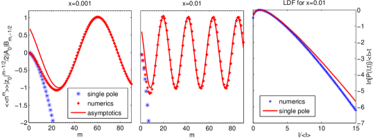
Figure 2: High-order cumulants and large deviation function for bunching transport through a two-level quantum dot. Left and central panels show comparisons between exact numerics and the single pole approximation stemming from Eq. (63) for two different values of $x=0.001,\,0.01$ and $\Gamma=0.01$. The asymptotic expression in Eq. (61) based on a pair of complex conjugate singularities is shown with full lines. Notice that $B_{m,-1/2}<0$. The right panel shows a comparison of the large deviation function (LDF) obtained from exact numerics and the single pole approximation in Eq. (71), respectively.

As anticipated above, these deviations can be traced back to the expression in Eq. (63), that we obtained in the limit $x,\Gamma\ll 1$. In order to proceed from here, we return to the full expression for the CGF in the long-time limit (not shown). A careful analysis reveals that, in fact, there is a pair of complex conjugate singularities closest to zero, and not just a single pole. The two singularities, denoted as $i\tilde{\chi}_{0}$ and $(i\tilde{\chi}_{0})^{*}$, correspond to branch points of a square-root, and for small $x\ll 1$ the position of the branch point $i\tilde{\chi}_{0}$ is

$$i\tilde{\chi}_{0}=\ln(2+\Gamma)-2x\frac{4+\Gamma(6+\Gamma)}{(2+\Gamma)^{2}}+4i\sqrt{x}\frac{1+\Gamma}{2+\Gamma}.$$ (67)

Clearly, for small $x,\Gamma\ll 1$ the branch points are close to the position of the single pole $i\chi_{0}=\ln 2$. However, for any finite $x$, the two branch points have small, but finite, imaginary parts thus complying with the Perron-Frobenius theorem. The singularity structure around the branch point $i\tilde{\chi}_{0}$ is characterized by Eq. (56) with $\mu_{0}=-1/2$ and $A_{0}\approx\Gamma t\sqrt[4]{x}e^{i\pi/4}$, and we can then use the asymptotic expressions in Eq. (61) for the high-order cumulants. In the left and central panels of Fig. 2 we compare this expression, and the single-pole approximation in Eq. (66), with numerically exact results obtained using our recursive scheme for $\Gamma=0.01$ and two different values of $x=0.001,\,0.01$.

Figure 2 shows several important features. Firstly, the (scaled) high-order cumulants indeed behave in an oscillatory manner as function of the cumulant order $m$, which coincides with the cosine part of Eq. (61). Obviously, for smaller $x=0.001$ the period of the oscillations, determined by $\arg i\tilde{\chi}_{0}$, is longer in accordance with Eq. (61). Furthermore, for the small value of $x=0.001$, the asymptotic form of the high-order cumulants is reached around $m\simeq 30$, while the single-pole approximation agrees well for lower orders, $m\lesssim 10$. For the higher value of $x=0.01$, significant deviations from the single-pole behavior begin already for the fourth cumulant, while the asymptotic oscillatory form holds from around $m=12$. Notice the importance of the exact analytical knowledge of the singularities — even though $x=0.01\ll 1$ (together with $\Gamma=0.01\ll 1$) may seem a very small number justifying the usage of the single pole approximation, we see from Eq. (67) that the imaginary part of the pole and its argument scale like $\sqrt{x}=0.1$, thus invalidating the single-pole approximation far earlier than expected from a linear-in-$x$ scaling assumption.

A complementary view on the charge transport statistics is provided by the large deviation function (LDF),Touchette (2009) which quantifies deviations of measurable currents from the average value. The LDF is obtained from the probability distribution

$$P(n,t)=\frac{1}{2\pi}\int_{-\pi}^{\pi}d\chi e^{S(\chi,t)-in\chi}$$ (68)

and is defined as the long-time limit of $\ln[P(I,t)]/t$, where $I\equiv n/t$ is the current. For long times, we have $S(\chi,t)\rightarrow\lambda_{0}(\chi)t$ and the integral can be evaluated in the saddle-point approximation with the saddle-point $\chi=\chi_{0}$ given by the solution to the saddle-point equation

$$\lambda_{0}^{\prime}(\chi_{0})=iI,$$ (69)

The saddle-point equation implies a parametric dependence of the saddle-point $\chi_{0}=\chi_{0}(I)$ on the current $I$. Using the saddle-point approximation, the LDF becomes

$$\frac{\ln[P(I,t)]}{t}\rightarrow\lambda_{0}(\chi_{0})-iI\chi_{0}.$$ (70)

We first solve the saddle-point equation for the approximate CGF in Eq. (63) and find

$$\frac{\ln[P_{1s}(I,t)]}{\langle I\rangle t}\rightarrow\frac{\sqrt{1+8\kappa}-3}{4}-\kappa\log\left[\frac{16\kappa}{(1+\sqrt{1+8\kappa})^{2}}\right],$$ (71)

where $\kappa\equiv I/\langle I\rangle$ and the subscript _1s again reminds us that the expression has been obtained using the approximate CGF with only a single singularity closest to zero. Obviously, the current must be positive ($\kappa>0$), since transport is unidirectional.

Also for the LDF, we can compare the analytic approximation with numerical exact results. To this end, we need to solve the saddle-point equation taking as starting point the kernel in Eq. (62). The derivative of the eigenvalue $\lambda_{0}(\chi)$ is now calculated using the Hellman-Feynman theorem, writing

$$\begin{split}\lambda_{0}^{\prime}(\chi)&=\frac{\partial}{\partial\chi}\langle\!\langle\tilde{0}(\chi)|\mathcal{W}(\chi)|0(\chi)\rangle\!\rangle\\ &=\langle\!\langle\tilde{0}(\chi)|\mathcal{W}^{\prime}(\chi)|0(\chi)\rangle\!\rangle,\end{split}$$ (72)

where $\langle\!\langle\tilde{0}(\chi)|$ and $|0(\chi)\rangle\!\rangle$ are left and right eigenvectors of $\mathcal{W}(\chi)$, respectively, corresponding to the eigenvalue $\lambda_{0}(\chi)$, and $\langle\!\langle\tilde{0}(\chi)|0(\chi)\rangle\!\rangle=1$. For a given value of $\chi$ we calculate numerically the left and right eigenvectors $\langle\!\langle\tilde{0}(\chi)|$ and $|0(\chi)\rangle\!\rangle$ and find $\lambda_{0}^{\prime}(\chi)$ using the expression for the derivative in Eq. (72). With this procedure we search numerically for the value of $\chi=\chi_{0}$ that solves Eq. (69) for a given value of $I$, and with the solution $\chi_{0}$ we evaluate the LDF using Eq. (70). We find that $\chi_{0}$ is purely imaginary.Bagrets and Nazarov (2003) We note that, in principle, the existence of a saddle point solution is not guaranteed in the whole range of currents, and there are examples,Bagrets et al. (2006); Visco (2006) where the behavior of the LDF changes abruptly at finite values of $I$ due to singularities of the CGF on the real $i\chi$-axis. In our case, however, the Perron-Frobenius theorem ensures that the CGF is analytic on the real $i\chi$-axis and the LDF is smooth as function of $I$. In the right panel of Fig. 2 we show a comparison between exact numerics and the analytic result (71) for the large deviation function in the single pole approximation. Around the mean value $I\simeq\langle I\rangle$ the analytic result agrees well with numerics. However, in the tails of the distribution a clear disagreement between the analytic approximation and numerics is visible. The disagreement reflects the deviations for the cumulants seen in the central panel of Fig. 2. We remark that measurements of the LDF recently have become accessible in experiments on real-time electron counting.Fricke et al. (2010)

The discussion in this subsection illustrates the need for careful considerations when manipulating CGFs analytically. Concerning cumulants, we deal with two opposite and non-commutative orders of limits: for a fixed order of cumulants, a limiting procedure with changing parameters converges to the approximate form given by the appropriate limit of the CGF, such as the single-pole approximation in Eq. (63) in our case. However, the convergence of the CGF is not uniform in $\chi$ due to potential singularities and thus for fixed parameters, high order cumulants generically take on the universal oscillatory form discussed above. One should thus be careful when using limiting forms of a CGF to extract cumulants of arbitrary orders. In general, the low-order cumulants follow the predicted pattern reasonably well, but at some point significant deviations appear and the universal oscillatory behavior should emerge. The order at which this crossover occurs depends on details of the analytical structure of the CGF and may be hard to predict. As we have shown explicitly, deviations of the cumulants from exact results are also clearly visible in the large deviation function.

V.2 Transport through a vibrating molecule

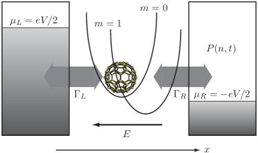
Figure 3: (color online). Transport through vibrating molecule. The molecule is coupled to the left (right) lead with coupling $\Gamma_{L}$ ($\Gamma_{R}$). The bias difference $eV=\mu_{L}-\mu_{R}$ drives single electrons through the molecule. The system is operated in the Coulomb blockade regime, where only $m=0$ or $m=1$ additional electrons are allowed on the molecule. As an electron tunnels onto the molecule, the equilibrium position of the molecule is shifted due to the electric field $E$. The two harmonic potentials corresponding to $m=0,1$ are shown. The damping rate of the vibrating molecule is denoted as $K$.

In our next example, we consider a model of charge transport through a molecule coupled to quantized vibrations.McCarthy et al. (2003); Mitra et al. (2004); Boese and Schoeller (2001); Flindt et al. (2005a); Koch and von Oppen (2005); Koch et al. (2005); Haupt et al. (2006) In the regime of weak coupling to the electronic leads, electron tunneling can be described using Fermi’s golden rule rates for transitions between different vibrational and charge occupation states. For strong electron-phonon coupling, the large shift of the oscillator equilibrium position due to an electron tunneling onto the molecule suppresses the (Franck-Condon) overlap between the initial and final vibrational state for low-lying oscillator states. This leads to surpressed tunnel rates at low bias-voltages, so-called Franck-Condon blockade. For larger bias-voltages, higher-excited oscillator states become available, and the system can escape the blockade regime. For weak oscillator dampings, several electrons can be transferred through the molecule, once the blockade is lifted, until a charge transfer event eventually leaves the oscillator in the ground state and the current is suppressed again. Such dynamical Franck-Condon blockade processes have been predicted to lead to very large enhancements of the zero-frequency noise.Koch and von Oppen (2005) Recently, Frank-Condon blockade was observed in experiments on suspended carbon nanotube quantum dots.Leturcq et al. (2009)

The system considered in the following is depicted in Fig. 3. Here we follow to a large extent the description of the model given in Refs. McCarthy et al., 2003, Flindt et al., 2005a. The Hamiltonian of the system and the detailed derivation of the resulting Markovian GME are given in App. B, where the various parameters of the model are also defined. Due to the large number of oscillator states, there is little hope for obtaining a closed-form expression for the CGF that would allow for any analytic manipulations. Instead, as we shall see, the numerically evaluated high-order cumulants can be used to extract the precise location of the dominating singularities of the CGF. We concentrate in the following on the unequilibrated oscillator regime, where the damping rate of the oscillator is much smaller than the electron tunneling rates, $K\ll\Gamma_{L/R}$. As explained above, the combination of strong electron-phonon coupling and weak oscillator damping leads to dynamical Franck-Condon blockade, resulting in a large enhancement of the current noise as demonstrated in Ref. Koch and von Oppen, 2005 using Monte-Carlo simulations. In Ref. Koch et al., 2005 the analysis was extended to the full distribution of the transferred charge and an analytic approximation for the CGF was presented based on an avalanche-type of transport, where “quiet” periods of transport are interrupted by a sequel of self-similar charge avalanches. The analytic result for the CGF was shown to agree very well with Monte-Carlo simulations of the probability distribution $P(n,t)$. However, similarly to the previous example, the approximate CGF has a single, simple pole on the real-$i\chi$ axis, violating the required properties of the CGF, mentioned at the end of Sec. IV, thus making it unsuited for predictions of the high-order cumulants. In particular, within this approximation, the high-order cumulants would not oscillate, which contradicts our numerical findings.

Oscillations of the high-order cumulants with system parameters must be due to singularities located away from the real-$i\chi$. In the following, we assume that the CGF has a pair of complex-conjugate singularities, $i\chi_{0}=|i\chi_{0}|e^{i\arg i\chi_{0}}$ and $|i\chi_{0}|e^{-i\arg i\chi_{0}}$, closest to zero. As we will now show, the positions of these singularities can be found from our numerical calculations of high-order cumulants. To this end, we define

$$a_{0}=A_{0}/(i\chi_{0})^{\mu_{0}}$$ (73)

and rewrite Eq. (61) as

$$\langle\!\langle n^{m}\rangle\!\rangle\simeq\!\frac{2|a_{0}|B_{m,\mu_{0}}}{|i\chi_{0}|^{m}}\cos\!\left[m\arg i\chi_{0}\!-\!\arg a_{0}\right].$$ (74)

Following the ideas of Ref. Zamastil and Vinette, 2005, Sec. 4, we find for the ratios of two successive cumulants

$$\begin{split}\frac{\langle\!\langle n^{m-1}\rangle\!\rangle}{\langle\!\langle n^{m}\rangle\!\rangle}\frac{m+\mu_{0}-1}{|i\chi_{0}|}&=\cos\!\left[\arg i\chi_{0}\right]\\ &+\sin\!\left[\arg i\chi_{0}\right]\tan\!\left[m\arg i\chi_{0}-\!\arg a_{0}\right]\end{split}$$ (75)

and

$$\begin{split}\frac{\langle\!\langle n^{m+1}\rangle\!\rangle}{\langle\!\langle n^{m}\rangle\!\rangle}\frac{|i\chi_{0}|}{m+\mu_{0}}&=\cos\!\left[\arg i\chi_{0}\right]\\ &-\sin\!\left[\arg i\chi_{0}\right]\tan\!\left[m\arg i\chi_{0}-\!\arg a_{0}\right].\end{split}$$ (76)

Adding the two left and right hand sides, respectively, and rearranging, we obtain the equation

$$\begin{split}2(m+\mu_{0})\langle\!\langle n^{m}\rangle\!\rangle|i\chi_{0}|\cos\!\left[\arg i\chi_{0}\right]-\langle\!\langle n^{m+1}\rangle\!\rangle|i\chi_{0}|^{2}=\\ \langle\!\langle n^{m-1}\rangle\!\rangle(m+\mu_{0}-1)(m+\mu_{0}).\end{split}$$ (77)

Using the substitution $m\rightarrow m+1$, we obtain an additional equation and thus arrive at a linear system of two equations which we solve for $|i\chi_{0}|\cos\!\left[\arg i\chi_{0}\right]$ and $|i\chi_{0}|^{2}$ and thereby find $i\chi_{0}$. The method takes as input $\langle\!\langle n^{m-1}\rangle\!\rangle$, $\langle\!\langle n^{m}\rangle\!\rangle$, $\langle\!\langle n^{m+1}\rangle\!\rangle$, and $\langle\!\langle n^{m+2}\rangle\!\rangle$, and the accuracy is expected to improve with increasing cumulant order $m$.Zamastil and Vinette (2005)

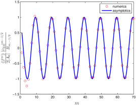
Figure 4: (color online). High-order (normalized) cumulants for unequilibrated molecule. Numerically exact results are shown together with the asymptotics described by Eq. (61). Parameters entering Eq. (61) are $\mu_{0}=-1/2$, $A_{0}=1.4810\times 10^{-7}e^{-i0.7378}$, and $i\chi_{0}=0.0113e^{i0.6262}$. System parameters (defined in App. B) are given in units of the natural oscillator frequency (with $e,\hbar,k_{B}=1$) $V=3\omega_{0}$, $\Gamma=\Gamma_{L}=\Gamma_{R}=0.001\omega_{0}$, $T=0.05\omega_{0}$, $K=10^{-10}\omega_{0}$, $\varepsilon=16\omega_{0}$, $c_{1}=4$, $c_{2}=0$. In the numerical calculations we have used $N=15$ oscillator states.

Having determined $i\chi_{0}$, we find $a_{0}$ in a similar spirit by rewriting Eq. (74) as

$$\begin{split}\langle\!\langle n^{m}\rangle\!\rangle\simeq&2B_{m,\mu_{0}}\left[\mathrm{Re}\{(i\chi_{0})^{-m}\}\mathrm{Re}\{a_{0}\}\right.\\ &\left.-\mathrm{Im}\{(i\chi_{0})^{-m}\}\mathrm{Im}\{a_{0}\}\right].\end{split}$$ (78)

Again, we obtain via the substitution $m\rightarrow m+1$ a linear system of two equations that we solve for $\mathrm{Re}\{a_{0}\}$ and $\mathrm{Im}\{a_{0}\}$ and thus find $a_{0}=\mathrm{Re}\{a_{0}\}+i\mathrm{Im}\{a_{0}\}$. Finally, we determine $A_{0}$ from Eq. (73). More advance methods for extracting the positions of singularities are available,Zamastil and Vinette (2005) but they require solutions of non-linear equations and will not be considered here.

In order to extract $i\chi_{0}$ and $A_{0}$ from the high-order cumulants, we need to know the nature of the singularities and hence $\mu_{0}$. Typically, the singularities are square-root branch points (see Ref. Bender and Orszag, 1999, Sec. 7.5) and we thus take $\mu_{0}=-1/2$. In Fig. 4 we show numerical results for the (normalized) cumulants as function of the order $m$ together with the asymptotic expression Eq. (61) for the high-order cumulants with $i\chi_{0}$ and $A_{0}$ found using the method described above. The asymptotic expression shows excellent agreement with the numerically exact results. For $m\gtrsim 5$, we see trigonometric oscillations whose frequency is determined by $\arg{i\chi_{0}}$. We note that a good agreement between our numerical results and the asymptotic expression could only be obtained with $\mu_{0}=-1/2$, thus confirming that the singularities stem from square-root branch points.

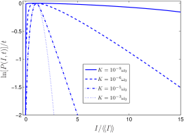
Figure 5: (color online). Large deviation function for the vibrating molecule. Results are shown for different values of the damping $K$, going from the unequilibrated regime, at low $K\ll\Gamma$, to $K\sim\Gamma$, where the molecule equilibrates between each tunneling event. For the unequilibrated case, a much larger range of currents are probable, compared to transport through the equilibrated molecule. System parameters (defined in App. B) are given in units of the natural oscillator frequency (with $e,\hbar,k_{B}=1$) $V=3\omega_{0}$, $\Gamma_{L}=\Gamma_{R}=0.001\omega_{0}$, $T=0.05\omega_{0}$, $\varepsilon=16\omega_{0}$, $c_{1}=4$, $c_{2}=0$.

The large deviation function can also be evaluated numerically using the method described in the previous subsection. In Fig. 5 we show numerical results for the large deviation function with different values of the damping $K$. For large dampings, the oscillator is essentially equilibrated and the measurable currents are closely centered around the mean current $\langle\!\langle I\rangle\!\rangle$. As the damping is lowered, we approach the unequilibrated regime, where the transport statistics is dominated by avalanche transport with a corresponding large zero-frequency noise. Accordingly, the large deviation function is considerably broadened and a much wider range of currents become measurable.

VI Non-Markovian systems

VI.1 Dissipative double quantum dot

In the previous two examples, we focused on the asymptotic behavior of the high-order cumulants for two Markovian systems. We now turn our attention to a model for which a weak coupling prescription does not suffice and non-Markovian effects become significant. We focus here on the influence of memory effects on the first few cumulants, while referring the reader to Ref. Flindt et al., 2008 for a discussion of the high-order cumulants for the non-Markovian system presented in this example.

We consider a model of charge transport through a double quantum dot (DQD) coupled to a heat bath which causes dephasing and relaxation. Such systems were studied experimentally in Refs. Fujisawa et al., 1998; Barthold et al., 2006. The counting statistics in the transition between coherent and sequential tunneling through DQDs has been studied theoretically by Kießlich and co-workers.Kießlich et al. (2006) In their work, decoherence was described using either a charge detector model or via phenomenological voltage probes.Blanter and Büttiker (2000) More elaborate descriptions of decoherence caused by a weakly coupled heat bath were given in Refs. Kießlich et al., 2007; Sánchez et al., 2008b and shown to agree well with experiments.

Here, we take these ideas further and go beyond the perturbative treatment of the heat bath. This situation has previously been investigated by Aguado and Brandes using a polaron transformation, assuming weak coupling to the electronic leads in the high-bias limit.Brandes and Kramer (1999); Aguado and Brandes (2004a, b) In the following, we apply an alternative non-perturbative scheme for the coupling to the heat bath, enabling us to fully include broadening due to the electronic leads. Within this approach, we can study the cross-over between weak and strong couplings to the heat bath and evaluate the effects of strong decoherence on the charge transport statistics. In particular, we show that only in the limit of weak coupling and high temperatures, the dephasing caused by the heat bath can be accounted for by a charge detector model with a single effective dephasing rate.

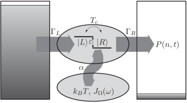
Figure 6: Dissipative double quantum dot. The Coulomb blockaded double quantum dot consists of the left and right levels $|L\rangle$ and $|R\rangle$, coherently coupled with tunnel coupling $T_{c}$ and dealigned by $\varepsilon$. A large bias across the system drives electrons through the double quantum dot from the left lead with rate $\Gamma_{L}$ to the right lead with rate $\Gamma_{R}$. The system is coupled with dissipation strength $\alpha$ to a heat bath at temperature $T$ and with Ohmic spectral function $J_{\Omega}(\omega)$. The probability distribution of the number of transferred charges $n$ is denoted $P(n,t)$.

The model of charge transport through a Coulomb blockaded DQDAguado and Brandes (2004a, b) is illustrated in Fig. 6. The DQD is coupled to source and drain electrodes, while dissipation is provided by an external heat bath. The DQD is operated in the Coulomb blockade regime close to a charge degeneracy point, where only a single additional electron is allowed on the double dot. Again, we consider for simplicity spinless electrons. The Hamiltonian of the double dot can be written

$$\hat{H}_{S}=\epsilon_{0}|0\rangle\!\langle 0|+\frac{\varepsilon}{2}\hat{s}_{z}+T_{c}\hat{s}_{x},$$ (79)

where the pseudo-spin operators are

$$\hat{s}_{z}\equiv|L\rangle\!\langle L|-|R\rangle\!\langle R|$$ (80)

and

$$\hat{s}_{x}\equiv|L\rangle\!\langle R|+|R\rangle\!\langle L|,$$ (81)

respectively. Here, the two quantum dot levels $|L\rangle$ and $|R\rangle$ are dealigned by $\varepsilon$ and their tunnel coupling is $T_{c}$. The energy of the ‘empty’ state $|0\rangle$ is $\epsilon_{0}$. The pseudo-spin interacts with an external heat bath consisting of harmonic oscillators,

$$\hat{H}_{B}=\sum_{j}\hbar\omega_{j}\hat{a}_{j}^{\dagger}\hat{a}_{j},$$ (82)

whose positions are coupled to the $z$-component of the pseudo-spin, adding the term $\hat{V}_{B}\hat{s}_{z}$ to the full Hamiltonian with

$$\hat{V}_{B}=\sum_{j}\frac{g_{j}}{2}(\hat{a}_{j}^{\dagger}+\hat{a}_{j}).$$ (83)

Finally, the spin-boson system is tunnel-coupled to left ($L$) and right ($R$) leads via the tunnel-Hamiltonian

$$\hat{H}_{T}=\sum_{k_{\alpha},\alpha=L,R}(t_{k_{\alpha}}\hat{c}^{\dagger}_{k_{\alpha}}|0\rangle\!\langle\alpha|+\mathrm{h.c.}),$$ (84)

with both leads described as non-interacting fermions, i.e.,

$$\hat{H}_{\alpha}=\sum_{k_{\alpha}}\varepsilon_{k_{\alpha}}\hat{c}^{\dagger}_{k_{\alpha}}\hat{c}_{k_{\alpha}},\,\,\,\alpha=L,R,$$ (85)

kept at chemical potentials $\mu_{\alpha}$, $\alpha=L,R$, and temperature $T$. The full Hamiltonian then reads

$$\hat{H}=\hat{H}_{S}+\hat{H}_{T}+\hat{H}_{L}+\hat{H}_{R}+\hat{H}_{B}+\hat{V}_{B}\hat{s}_{z}.$$ (86)

As previously pointed out,Aguado and Brandes (2004a, b) the model can be mapped onto that of transport through a superconducting single electron transistor, when the charging energy is much larger than the Josephson energy. Throughout this example we take $\hbar=k_{B}=e=1$.

As explained in App. C, transport through the double dot can be described using a non-Markovian equation of motion of the form in Eq. (1) for the three electronic occupations of the double dot collected in the vector $\hat{\rho}=(\rho_{0},\rho_{L},\rho_{R})^{T}$. The occupation probabilities of the empty, left, and right states, are denoted $\rho_{0}$, $\rho_{L}$, and $\rho_{R}$, respectively. The corresponding memory kernel in Laplace space reads

$$\mathcal{W}(\chi,z)=\begin{pmatrix}-\Gamma_{L}&0&\Gamma_{R}e^{i\chi}\\ \Gamma_{L}&-\Gamma_{B}^{(+)}(z)&\Gamma_{B}^{(-)}(z)\\ 0&\Gamma_{B}^{(+)}(z)&-\Gamma_{B}^{(-)}(z)-\Gamma_{R}\\ \end{pmatrix}.$$ (87)

We note that the kernel with $\chi=0$ has a single zero-eigenvalue $\lambda_{0}(0,z)=0$ for all $z$, in agreement with Eq. (14). The kernel has been derived under the assumption that the symmetrically applied bias $eV=|\mu_{L}-\mu_{R}|$ between the electronic leads is much larger than the tunneling rates to the leads and the temperature $T$. The tunneling rates are defined as

$$\Gamma_{\alpha}(\epsilon)=2\pi\sum_{k}|t_{k_{\alpha}}|^{2}\delta(\epsilon-\varepsilon_{k_{\alpha}}),\,\,\,\alpha=L,R,$$ (88)

and are assumed energy-independent, such that $\Gamma_{\alpha}(\epsilon)\equiv\Gamma_{\alpha}$, $\alpha=L,R$. We count the number of electrons that have been collected in the right lead, and consistently with this choice, the counting field $\chi$ has been introduced in the off-diagonal element of the memory kernel that contains the rate $\Gamma_{R}$.

The expressions for the bath-assisted hopping rates are derived in App. C and for real $z$ they read

$$\Gamma_{B}^{(\pm)}(z)=T_{c}^{2}[g^{(+)}(z_{\pm})+g^{(-)}(z_{\mp})],$$ (89)

where $z_{\pm}\equiv z\pm i\varepsilon+\Gamma_{R}/2$. These expression are valid to the lowest order in the tunnel coupling $T_{c}$. The bath-correlation functions in Laplace space are

$$g^{(\pm)}(z)=\int_{0}^{\infty}dte^{-W(\mp t)-zt}$$ (90)

withWeiss (2001)

$$W(t)=\int_{0}^{\infty}d\omega\frac{J(\omega)}{\omega^{2}}\{[1-\cos(\omega t)]\coth{(\beta\omega/2)}+i\sin(\omega t)\},$$ (91)

and

$$J(\omega)\equiv\sum_{j}|g_{j}|^{2}\delta(\omega-\omega_{j})$$ (92)

being the spectral function of the heat bath. In this work we consider Ohmic dissipation characterized by a coupling strength $\alpha$ such that the spectral function reads

$$J_{\Omega}(\omega)=2\alpha\omega e^{-\omega/\omega_{c}}.$$ (93)

where $\omega_{c}$ is the frequency cut-off, assumed to be the highest energy scale of the system.

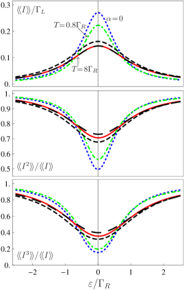
Figure 7: (color online). Cumulants for weakly coupled heat bath. The first three cumulants are shown as functions of the dealignment $\varepsilon$. We show results for a low ($T=0.8\Gamma_{R}$) and a high temperature ($T=8\Gamma_{R}$) as well as for the uncoupled case ($\alpha=0$). For the high temperature case, we compare with results obtained using a charge detector dephasing model (short-dashed black line) and results without inclusion of memory effects (long-dashed black line), see text. Parameters are $\Gamma_{L}=0.1\Gamma_{R}$, $T_{c}=0.1\Gamma_{R}$, $\alpha=0.01$, and $\omega_{c}=5\times 10^{4}\Gamma_{R}$, and thus $\Gamma_{d}\simeq 0.8\Gamma_{R}$ according to Eq. (94).

In Fig. 7 we show results for weak couplings to the heat bath, $\alpha\ll 1$. As the two quantum dot levels are tuned into resonance ($\varepsilon=0$), the current reaches a maximum with a width mainly determined by $\Gamma_{R}$. The corresponding values for the second and third cumulant, normalized with respect to the current, are suppressed below unity. The suppression is stronger for the third cumulant. Away from resonance, the mean current falls off, and the second and third cumulants approach unity, corresponding to a Poisson process. Without coupling to the heat bath, $\alpha=0$ (dotted blue line), the only broadening mechanism is the escape of electrons through the right barrier at rate $\Gamma_{R}$. This rate also defines the relevant energy scale to which we compare the temperature of the heat bath. Away from resonance, the uncoupled case captures well the results obtained at low temperatures, $T<\Gamma_{R}$. (dashed-dotted green line). At higher temperatures, $T\gg\Gamma_{R}$ (full red line), the peak in the current and the dips in the second and third cumulants are considerably broadened due to the strong temperature induced dephasing. Further results for the weak coupling limit are presented in Ref. Braggio et al., 2008.

In order to understand the behavior at high temperatures (full red line), we imagine replacing the heat bath by a charge detector which measures the position of electrons on the DQD, thereby causing dephasing.Gurvitz (1997); Kießlich et al. (2006); Braggio et al. (2009b) The effects of the charge detector can be described by a single dephasing rate $\Gamma_{d}$, entering as an additional exponential decay of the off-diagonal elements between the left and right quantum dot states. As we show in App. C, this picture follows from the high-temperature limit of the kernel in Eq. (87), and the corresponding dephasing rate is

$$\Gamma_{d}=2\alpha\pi T.$$ (94)

The dynamics of the system effectively becomes Markovian at high temperatures $T\gg\Gamma_{R}$, where the characteristic memory time $\sim(\Gamma_{R}/2+\Gamma_{d})^{-1}$ of the kernel is shorter than the timescale $\sim\Gamma_{R}^{-1}$ over which the populations of the DQD evolve. In Fig. 7 we see that the counting statistics at high temperatures (full red line) are well approximated by the charge detector model (short-dashed black line), which captures the broadening of the peak in the current and the dips in the second and third cumulants. For high temperatures (full red line), the large value of the dephasing rate indicates that the system is strongly dephased. The charge detector model, however, cannot account for the weak asymmetry between the phonon emission ($\varepsilon>0$) and absorption ($\varepsilon<0$) sides at low temperatures (dashed-dotted green line).

In our description of the DQD system we have traced out the electronic off-diagonal elements, the coherencies, together with the electronic leads and the heat bath. Our derivation allows us to combine strong coupling to the heat bath with broadening of the electronic levels due to the electrodes. However, even without coupling to the heat bath, the kernel must be time-dependent in order to account for the coherent oscillations between the left and right quantum dot states. These coherent effects are suppressed, when the dephasing is strong, and in that limit we thus expect that a Markovian description would suffice. We check this assumption by plotting in Fig. 7 only the Markovian parts of the cumulants at high temperatures (long-dashed black line). Away from resonance, the Markovian parts agree well for the second and third cumulants showing that the system at high temperatures effectively is Markovian. The mean current, as previously mentioned, is already a Markovian quantity and it coincides with the Markovian contribution as expected.Braggio et al. (2006) Closer to resonance, some deviations for the second and third cumulants are seen as the system is not completely dephased.

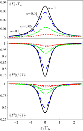
Figure 8: (color online). Cumulants in the intermediate regime between weak and strong coupling to the heat bath. The first three cumulants are shown as functions of the dealignment $\varepsilon$. The values of the coupling to the heat bath are $\alpha=0$, 0.01, 0.05, and 0.1. For large couplings ($\alpha=0.5,1$), we compare with results obtained without inclusion of memory effects (dot-dashed lines), see text. Parameters are $\Gamma_{L}=\Gamma_{R}$, $T_{c}=0.1\Gamma_{R}$, $T=0.5\Gamma_{R}$, and $\omega_{c}=5\times 10^{4}\Gamma_{R}$.

In Fig. 8 we show results for larger values of the coupling to the heat bath. Also in this case, the peak in the current and the dips in the second and third cumulants are suppressed as the coupling is increased and dephasing becomes stronger. Contrary to the weak coupling regime, however, no broadening of these features are observed. This is not consistent with the charge detector model, which would predict an increased width together with suppression of the height of the current peak and the depth of the dips in the second and third cumulants. Additionally, as the coupling $\alpha$ is increased, the emission/absorption asymmetry becomes stronger as exchange of energy quanta with the heat bath becomes increasingly important. As noted before, neither the absence of broadening nor the asymmetry of the peaks and dips can be accounted for by the charge detector model. For large values of the coupling to the heat bath, the DQD system completely dephases and the Markovian contribution describes well the behavior of the counting statistics, in particular away from resonance, where coherent effects are less relevant. At even larger couplings, the heat bath tends to localize electrons to one of the two quantum dots, and the effective tunnel rate between the two quantum dots becomes highly suppressed. In that case, the current through the system is very low and the statistics is Poissonian.

VI.2 Discussion of non-Markovian systems

We close this section by pointing out various possible subtleties associated with MarkovianDümcke and Spohn (1979); Kohen et al. (1997) and, in particular, non-MarkovianBarnett and Stenholm (2001) GMEs. As we shall argue, special attention should be paid to the sometimes paradoxical nature of heuristically derived non-Markovian GMEs (see e. g. Ref. Barnett and Stenholm, 2001) in order to ensure physically meaningful results. We moreover discuss the interpretation of the “mean memory time” for non-Markovian systems and we show that it in certain cases can turn negative. As an illustrative example, we consider unidirectional transport through a single electronic level. This generic model provides us with a unifying explanation of previous results obtained for several different systems and, in addition, it displays a few possible peculiarities of non-Markovian transport.

The Markovian master equation for the simple two-state model of unidirectional transport through a single electronic level is determined by the rate matrixBlanter and Büttiker (2000); Bagrets and Nazarov (2003); Gustavsson et al. (2006); Flindt et al. (2009)

$$\mathcal{W}(\chi)=\begin{pmatrix}-\Gamma_{L}&\Gamma_{R}e^{i\chi}\\ \Gamma_{L}&-\Gamma_{R}\end{pmatrix}$$ (95)

with the counting field $\chi$ corresponding to tunneling across the right barrier. An intuitive way to generalize the rate matrix to the non-Markovian case would be simply to replace the rates $\Gamma_{L/R}$ by time-dependent rates, so that the rate matrix in Laplace space instead reads

$$\mathcal{W}(\chi,z)=\begin{pmatrix}-\Gamma_{L}(z)&\Gamma_{R}(z)e^{i\chi}\\ \Gamma_{L}(z)&-\Gamma_{R}(z)\end{pmatrix}.$$ (96)

The non-Markovian character could be caused by external degrees of freedom that have been traced out, for example a harmonic oscillator mode coupled to the occupation of the electronic level, as studied in Sec. V.2. Alternatively, it could be due to an energy-dependent tunneling density of states as in Ref. Zedler et al., 2009, or many-body-induced effects as in the Fermi-edge-singularity problem in transport.Matveev and Larkin (1992); Hapke-Wurst et al. (2000); Frahm et al. (2006); Maire et al. (2007); Rüth et al. (2008)

The microscopic origin of the memory, however, is not important in the following and its effect on the current noise is qualitatively captured by the “mean memory times”

$$\tau_{L,R}\equiv-\left.\tfrac{d}{dz}\log\Gamma_{L,R}(z)\right|_{z=0}=\frac{\int_{0}^{\infty}t\Gamma_{L,R}(t)dt}{\int_{0}^{\infty}\Gamma_{L,R}(t)dt}.$$ (97)

If $\Gamma(t)\propto e^{-t/\tau}$ the mean memory time has a direct physical interpretation as the characteristic memory time $\tau$. However, the following statements are valid for any memory kernel as long as it has a finite mean memory time $\tau$. Using Eqs. (44,47) we find the following expression for the Fano factor [see also Eq. (13) of Ref. Flindt et al., 2007]

$$F=\frac{\langle\!\langle I^{2}\rangle\!\rangle}{\langle\!\langle I\rangle\!\rangle}=\frac{\Gamma_{L}^{2}+\Gamma_{R}^{2}}{(\Gamma_{L}+\Gamma_{R})^{2}}-2\frac{\Gamma_{L}^{2}\Gamma_{R}\tau_{R}+\Gamma_{R}^{2}\Gamma_{L}\tau_{L}}{(\Gamma_{L}+\Gamma_{R})^{2}}$$ (98)

where $\Gamma_{L,R}\equiv\Gamma_{L,R}(z=0)>0$ is the Markovian limit of the rates. The second term is a non-Markovian correction to the well-known expression for the Fano factor of transport through a single electronic level.Blanter and Büttiker (2000) For certain parameter values, however, this non-Markovian correction can make the Fano factor turn negative — a clearly unphysical result (the zero-frequency noise must be positive, see e.g. Refs. Blanter and Büttiker, 2000; Flindt et al., 2004). We discuss this issue in further detail below.

Obviously, different baths producing the same mean memory times give rise to the same electronic noise. Intuitively, one would also expect the mean memory times to be positive. Since the Markovian limit of the $\Gamma$’s must be positive (being rates) the non-Markovian correction appears negative; thus the general effect of memory on transport through a single level is a decrease of the noise compared to the corresponding Markovian limit. This statement is in line with a number of previous findings: It explains the anomalous suppression of the Fano factor below $1/2$ in transport through a single electronic level coupled to a mechanical resonator reported in Ref. Haupt et al., 2006. Additionally, the non-Markovian correction due to strong spectral features in the Fermi edge singularity problemMatveev and Larkin (1992); Hapke-Wurst et al. (2000); Frahm et al. (2006); Rüth et al. (2008) is responsible for the observed discrepancyMaire et al. (2007) between the measured Fano factor and the expected result based on the Markovian part only. A more detailed account of this problem will be presented elsewhere.Roszak and Novotný Finally, the suppression of the Fano factor compared to the Markovian approximation is also confirmed by the study of an exactly solvable caseZedler et al. (2009) in the regime where the non-Markovian GME provides a good approximation to the exact dynamics.

Although the above expression (98) provides a unifying explanation of these three examples, it obviously cannot be correct in general as mentioned above. For weak non-Markovian behavior, where the $\tau$’s are small, the Fano factor stays positive, and the non-Markovian corrections lead to a reduction of noise. In general, however, there is no guaranty that the Fano factor in Eq. (98) is always non-negative. This can be traced back to the heuristic inclusion of the non-Markovian kernel in Eq. (96). While the non-Markovian kernel for unidirectional transport through a single level in general may be written in the form (96) without counting fields, the inclusion of the counting field must be carried out carefully, for example by using well-controlled systematic derivation procedures, such as those based on perturbation theories.Braggio et al. (2006) Non-Markovian GMEs may, however, still lead to unphysical results, when employed outside their regime of validity, as recently discussed by Zedler and co-workers.Zedler et al. (2009) In the Markovian case, the heuristic addition of the counting field in $\mathcal{W}$ usually leads to correct results for the counting statistics, although exceptions do exist.Prachař and Novotný (2010) In the non-Markovian double dot system studied in Sec. VI.1, the counting field enters the Markovian ($z$-independent) part of kernel in Eq. (87), and the inclusion of the counting field does not lead to any of the issues discussed above.

Finally, we discuss another subtlety associated with strongly non-Markovian systems. Under certain circumstances the mean memory time $\tau$, defined in Eq. (97) may in fact become negative. This happens for example for the dissipative double quantum dot studied in Sec. VI.1. For a sufficiently small dissipation rate, we find for the bath-assisted rates $\partial_{z}\Gamma_{B}^{(\pm)}(z=0)>0$, resulting in negative mean memory times. Formally, there is no problem associated with this phenomenon (the GME still describes a positivity-preserving evolution), but the physical interpretation of the non-Markovian corrections is less clear due to this counterintuitive behavior. The problem is purely interpretation-related and concerns the issue of a proper Markovian limit.

In cases with large memory effects, the formal Markovian limit, corresponding to $\mathcal{W}(z\rightarrow 0)$, does not give a reasonable description of the system dynamics, although it yields correct stationary quantities, like the mean current. Since the noise (and also higher-order cumulants) is a time integral of a transient quantity, namely a current-current correlation function, the formal Markovian limit of the noise in these cases is a somewhat unphysical quantity. The problems with the interpretation of a Markovian limit also influence the interpretation of the non-Markovian corrections (via, e. g. negative memory times). Bluntly, a physically meaningful result is arbitrarily split into two additive parts, Markovian and non-Markovian, that each do not necessarily have a reasonable physical interpretation. The full result, however, is correct and physically plausible. These effects are well illustrated and can be understood by studying exactly solvable cases such as the one in Ref. Zedler et al., 2009.

In this section, we have only briefly touched upon various open questions and subtleties associated with interpretations of non-Markovian dynamics. However, the exact method developed in this paper paves the way for future systematic studies of memory effects in connection with electronic noise and counting statistics.

VII Conclusions

We have presented a detailed derivation of a recursive scheme for evaluating high-order cumulants of transport through Coulomb-blockade nanostructures with many states and non-Markovian dynamics. In order to illustrate the use of our method for Markovian systems we considered the counting statistics of transport through a two-level quantum dot and a vibrating molecule. In both cases, we have shown how the behavior of high-order cumulants is determined by dominating singularities of the cumulant generating functions. Oscillations of the high-order cumulants as function of the cumulant order can be used to locate the positions of singularities as we have demonstrated. We have also calculated the distribution of measurable currents, the so-called large deviation function, and shown how the tails of the distributions reflect the high-order cumulants. In order to illustrate the use of our method for a non-Markovian system, we considered transport through a dissipative double quantum dot. For this system, we have studied how bath-induced dephasing affects the first three cumulants and found that effects of the heat bath cannot be accounted for by an effective detector model, when the coupling becomes strong. Finally, we have discussed the nature and significance of non-Markovian dynamics in relation to counting statistics.

The research presented in this work points to several interesting directions to follow. While we have focused on the zero-frequency current cumulants of non-Markovian processes, it would be interesting to see, if the methods presented here could be extended to finite frequencies, as it was recently done for Markovian processes.Emary et al. (2007) It has now been firmly established that high-order cumulants of the counting statistics generally grow factorially with the cumulant order and oscillate as functions of basically any system parameters as well as of the cumulant order. It would be interesting to study in further detail how microscopic details of a system are reflected, for example, in the frequency of these oscillations. Such a study would shed new light on the information contained in high-order cumulants. Finally, we believe that the methods presented here will pave the way for future systematic studies of counting statistics in connection with non-Markovian dynamics.

Appendix A QR decomposition

In this appendix we present technical details of one possible method for evaluating Eqs. (48) and (52) in Sec. III.2. The method we use is a standard technique in numerical linear algebra known as QR decomposition. Routines performing QR decompositions are a part of most common linear algebra packages such as LAPACK. Below we provide a piece of code implemented in MATLAB and subsequently explain in detail each step of the code, such that it can be reproduced in other programming languages (MATLAB itself uses an implementation of the QR decomposition from the underlying LAPACK library). The code is written in a general way but there are steps which are specific to the particular model considered here — those program lines are explicitly denoted. As a model system we use a double dot with 5 retained elements of the density matrix $\hat{\rho}$ and corresponding vector representation

$$|\rho\rangle\!\rangle=[\rho_{00},\rho_{LL},\rho_{RR},\rho_{LR},\rho_{RL}]$$ (99)

. The trace of the density matrix can then be written

$$\mathrm{Tr}\{\hat{\rho}\}=\langle\!\langle\tilde{0}|\rho\rangle\!\rangle=\rho_{00}+\rho_{LL}+\rho_{RR}$$ (100)

with

$$\langle\!\langle\tilde{0}|=[1,1,1,0,0]^{T}.$$ (101)

The excerpt of the code for the evaluation of the stationary state Eq. (48) and the pseudo-inverse (modification of Eq. (52))

$$\mathcal{WR}=\mathcal{Q}$$ (102)

reads:

% Size of the Liouville space
N = length(W(:,1));

% Left zero eigenvector (MODEL DEPENDENT)
%  Here for a double dot
trace=[1,1,1,0,0];

% QR decomposition with sorting the diagonal
%  elements of ’r’ in descending order
%  (built-in routine from LAPACK)
[q,r,e] = qr(W);

% Consistency check - when the matrix ’W’ is
%  singular the last row of the matrix ’r’
%  should be zero
tol = 1e-10;    % Setting the tolerance
if max(r(end,:))>tol
     warning(’Last row of r is non-zero’)
     display(r(end,:))
end

% Stationary state
stat = e*[r(1:N-1,1:N-1) \ r(1:N-1,end); -1];

% Normalization of the stationary state
stat = stat/(trace*stat);

% Projectors
P = kron(stat,trace); Q = eye(N) - P;

% Solution of the pseudo-inverse equation
temp = q \ Q;

% Consistency check - if the matrix ’Q’ is
%  a projector onto the regular space of ’W’,
%  the solvability condition requires the
%  last column of the matrix ’temp’ to be zero
if max(temp(end,:))>tol
    warning(’Last row is non-zero’)
    display(max(temp(end,:)))
end

% Finding a particular solution of the equation
X = e*[r(1:N-1,1:N-1)\temp(1:N-1,:);zeros(1,N)];

% Final fixing of the pseudo-inverse by
%  multiplication by the projector ’Q’
R = Q*X;

The code can be understood by first analyzing the structure of the output from the QR decomposition routine. The QR routine takes as input a matrix $\mathbf{W}$ of dimension $N\times N$. The output consists of three matrices of same dimension $\mathbf{q},\,\mathbf{e},\,\mathbf{r}$, such that $\mathbf{q}\cdot\mathbf{r}=\mathbf{W}\cdot\mathbf{e}$. Here, $\mathbf{q}$ is a unitary (and thus regular) matrix, $\mathbf{e}$ a permutation matrix (thus also regular), and $\mathbf{r}$ an upper triangular matrix with decreasing diagonal elements. The column permutation matrix $\mathbf{e}$ is chosen such that $\mathrm{abs}(\mathrm{diag}(\mathbf{r}))$ is decreasing. For a singular matrix $\mathbf{W}$ representing $\mathcal{W}$, this implies that the last diagonal entry of $\mathbf{r}$ is zero and, therefore, the last row of $\mathbf{r}$ is zero. More explicitly, we have

$$\mathbf{r} =\begin{pmatrix}r_{1,1}&r_{1,2}&r_{1,3}&r_{1,4}&\dots&r_{1,N}\\ 0&r_{2,2}&r_{2,3}&r_{2,4}&\dots&r_{2,N}\\ 0&0&r_{33}&r_{3,4}&\dots&r_{3,N}\\ \vdots&\vdots&\vdots&\ddots&\ddots&\vdots\\ 0&0&\dots&0&r_{N-1,N-1}&r_{N-1,N}\\ 0&0&0&0&0&0\\ \end{pmatrix}$$ (103a)

$$=\begin{pmatrix}[\mathbf{\tilde{r}}]_{N-1\times N-1}&[\mathbf{r^{\prime}}]_{N-1\times 1}\\ [0]_{1\times N-1}&0\end{pmatrix}$$ (103b)

with $\mathbf{\tilde{r}}$ being an upper triangular matrix with non-zero diagonal and dimension $(N-1)\times(N-1)$ and $\mathbf{r^{\prime}}$ a column vector of length $N-1$. The QR decomposition of $\mathcal{W}$ implies for the solution $|0\rangle\!\rangle$ to the matrix implementation of Eq. (48) that

$$\mathbf{W}\cdot\mathbf{0}=\left(\mathbf{q}\cdot\mathbf{r}\cdot\mathbf{e}^{-1}\right)\cdot\mathbf{0}=0\ \Rightarrow\ \mathbf{r}\cdot\left(\mathbf{e}^{-1}\cdot\mathbf{0}\right)=0.$$ (104)

Here, $\mathbf{0}$ is a vector representation of $|0\rangle\!\rangle$, named stat in the code.

The block structure of the matrix $\mathbf{r}$ depicted in Eq. (103b) shows that $(\mathbf{e}^{-1}\cdot\mathbf{0})=c[\mathbf{\tilde{r}}^{-1}\cdot\mathbf{r^{\prime}},-1]^{T}$ for any number $c$ is a solution to the matrix equation above. We then find $\mathbf{0}=c\mathbf{e}\cdot[\mathbf{\tilde{r}}^{-1}\cdot\mathbf{r^{\prime}},-1]^{T}$ with $c=1/(\mathbf{\tilde{0}}\cdot\mathbf{e}\cdot[\mathbf{\tilde{r}}^{-1}\cdot\mathbf{r^{\prime}},-1]^{T})$, ensuring the proper normalization $\mathbf{\tilde{0}}\cdot\mathbf{0}=1$. We note that the only model dependent part of the code is the definition of the left zero eigenvector $\mathbf{\tilde{0}}$ named trace in the code.

Next, we determine the pseudo-inverse $\mathbf{R}$. To this end, we form the projectors $\mathbf{P}=\mathbf{0}\otimes\mathbf{\tilde{0}}$ and $\mathbf{Q}=\mathbf{1}-\mathbf{P}$. For the Kronecker tensor product, the code uses the built-in function kron(,). Equation (102) can now be expressed in matrix form as

$$\mathbf{W}\cdot\mathbf{R}=\left(\mathbf{q}\cdot\mathbf{r}\cdot\mathbf{e}^{-1}\right)\cdot\mathbf{R}=\mathbf{Q}\ \Rightarrow\ \mathbf{r}\cdot\left(\mathbf{e}^{-1}\cdot\mathbf{R}\right)=\mathbf{q}^{-1}\cdot\mathbf{Q}$$

Since the right hand side $\mathcal{Q}$ of the original equation (102) lies in the range of $\mathcal{W}$ the resulting matrix equation for $\left(\mathbf{e}^{-1}\cdot\mathbf{R}\right)$ above must have a solution. This requires that the last row of $\mathbf{q}^{-1}\cdot\mathbf{Q}$ is zero as follows again from the block structure of $\mathbf{r}$ shown in Eq. (103b) (this condition is explicitly checked for in the code). A particular solution of the equation is then $\begin{pmatrix}\mathbf{\tilde{r}}^{-1}\cdot[\mathbf{A}]_{N-1\times N}\\ [0]_{1\times N}\end{pmatrix}$ with the rectangular matrix $\mathbf{A}$ being a restriction of the product $\mathbf{q}^{-1}\cdot\mathbf{Q}$ to the $(N-1)$ first rows. The pseudo-inverse is now fixed by multiplying this particular solution by the permutation matrix $\mathbf{e}$ and finally by the projector $\mathbf{Q}$ as follows from the discussion below Eq. (53).

We have used the code on a standard PC for all of the examples shown in this paper and it is efficient both in terms of memory and CPU time for $N\times N$ matrices with $N$ being up to several thousands. For larger matrices, the direct evaluation of the pseudo-inverse becomes prohibited both in terms of memory as well as CPU time and one should use other methods such as, e.g., the iterative Arnoldi scheme described in detail in App. A of Ref. Flindt et al., 2004.

Appendix B Vibrating molecule

In this appendix we describe the model of a vibrating molecule considered in Sec. V.2 and derive the corresponding Markovian GME. Here we follow to a large extent the description of the model given in Refs. McCarthy et al., 2003, Flindt et al., 2005a. The molecule is operated in the Coulomb blockade regime, where only two charge states ($m=0$ or $m=1$ additional electrons on the molecule) participate in the transport. We consider spinless electrons with charge $-e$, although it would be easy to include the spin degree of freedom. The Hamiltonian of the molecule is

$$\hat{H}_{S}=\frac{\hat{p}^{2}}{2m_{0}}+\frac{1}{2}m_{0}\omega_{0}^{2}\hat{x}^{2}+(\varepsilon-eE\hat{x})\hat{d}^{\dagger}\hat{d},$$ (105)

where $E$ is the electric field at the position of the molecule with mass $m_{0}$ and natural oscillator frequency $\omega_{0}$. The electric field is determined by the bias across the molecule and bias-independent contributions, e.g., image-charge effects. The charging energy difference between 0 and 1 additional electron on the molecule is denoted as $\varepsilon$. The molecule is tunnel-coupled to left and right electrodes consisting of non-interacting fermions

$$\hat{H}_{\alpha}=\sum_{k_{\alpha}}\varepsilon_{k_{\alpha}}\hat{c}^{\dagger}_{k_{\alpha}}\hat{c}_{k_{\alpha}},\,\,\alpha=L,R,$$ (106)

kept at chemical potentials $\mu_{\alpha}$, $\alpha=L,R$, and temperature $T$. Tunneling processes are accounted for by a standard tunnel-Hamiltonian

$$\hat{H}_{T}=\sum_{k_{\alpha},\alpha=L,R}\left(t_{k_{\alpha}}\hat{c}^{\dagger}_{k_{\alpha}}\hat{d}+\mathrm{h.c.}\right).$$ (107)

For simplicity, we neglect any position dependence of the tunneling amplitudes $t_{k_{\alpha}}$, but it would be straightforward to include.McCarthy et al. (2003) Finally, damping of the mechanical oscillations are described by coupling to a bath of oscillators, such that the full Hamiltonian reads

$$\hat{H}=\hat{H}_{S}+\hat{H}_{T}+\hat{H}_{L}+\hat{H}_{R}+\hat{x}\hat{V}_{B}+\hat{H}_{B},$$ (108)

where

$$\hat{V}_{B}=\sum_{j}\frac{g_{j}}{2}(\hat{a}^{\dagger}_{j}+\hat{a}_{j}),$$ (109)

and

$$\hat{H}_{B}=\sum_{j}\hbar\omega_{j}\hat{a}^{\dagger}_{j}\hat{a}_{j}.$$ (110)

The coupling to the $j$’th oscillator, with frequency $\omega_{j}$ and corresponding creation and annihilation operators $\hat{a}^{\dagger}_{j}$ and $\hat{a}_{j}$, respectively, is denoted $g_{j}$.

We treat both the coupling to the electronic leads and the heat bath in the weak coupling approximation and it thus suffices to consider the time evolution of the diagonal matrix elements of the reduced density matrix of the charge and oscillator states of the molecule. These diagonal elements correspond to the energy eigenstates of the isolated molecule described by $\hat{H}_{S}$. The eigenstates with $m=0$ additional electrons on the molecule are

$$|m=0,l\rangle=|\mathrm{empty}\rangle\otimes|l\rangle$$ (111)

with corresponding eigenenergies

$$E_{0l}=\hbar\omega_{0}\left(l+\frac{1}{2}\right).$$ (112)

Here, $|\mathrm{empty}\rangle$ denotes the empty charge state, while $|l\rangle=(\hat{a}^{\dagger})^{l}|0\rangle/\sqrt{l!}$ is the $l$’th oscillator state centered at $x=0$. The operator $\hat{a}^{(\dagger)}$ lowers (raises) the oscillator number by 1 and $|0\rangle$ is the oscillator ground state. With $m=1$ additional electron on the molecule the equilibrium position of the oscillator is shifted by the distance $d=eE/m_{0}\omega_{0}^{2}$. The eigenstates for the occupied molecule are thus

$$|m=1,l\rangle=|\mathrm{occupied}\rangle\otimes e^{\gamma(\hat{a}^{\dagger}-\hat{a})}|l\rangle,$$ (113)

where we have introduced the dimensionless electron-phonon coupling

$$\gamma=\frac{eEx_{0}}{\hbar\omega_{0}}$$ (114)

with $x_{0}=\sqrt{\hbar/2m_{0}\omega_{0}}$. The corresponding eigenenergies are

$$E_{1l}=\varepsilon+\hbar\omega_{0}\left(l+\frac{1}{2}\right)-\gamma^{2}\hbar\omega_{0}.$$ (115)

In the following we denote the diagonal elements of the reduced density matrix by $\rho_{m,l}(n,t)$, where $n$ is the number of electrons collected in the right electrode during the time span $[0,t]$. Bath-mediated transitions between different vibrational states are given by the thermal ratesMcCarthy et al. (2003)

$$W_{l+1\leftarrow l}=W_{l\leftarrow l+1}e^{-\beta\hbar\omega_{0}}=K\frac{\hbar(l+1)}{e^{\beta\hbar\omega_{0}}-1},$$ (116)

where $K$ characterizes the vibrational damping rate and $\beta=1/k_{B}T$ is the inverse temperature. The charge transfer rates, obtained using Fermi’s Golden rule, are

$$\begin{split}\Gamma_{1,l^{\prime}\leftarrow 0,l}^{(s)}&=\Gamma_{(s)}|F_{l^{\prime}l}|^{2}f(E^{(s)}_{ll^{\prime}}),\\ \Gamma_{0,l\leftarrow 1,l^{\prime}}^{(s)}&=\Gamma_{(s)}|F_{ll^{\prime}}|^{2}[1-f(E^{(s)}_{ll^{\prime}})],\end{split}$$ (117)

where $f$ is the Fermi function, $\Gamma_{(+1/-1)}=\Gamma_{L/R}$ are the bare tunneling rates, which are assumed to be energy independent, i. e.

$$\Gamma_{\alpha}=\Gamma_{\alpha}(\epsilon)=2\pi\sum_{k_{\alpha}}|t_{k_{\alpha}}|^{2}\delta(\epsilon-\varepsilon_{k_{\alpha}}),\,\,\alpha=L,R.$$ (118)

Moreover, we have defined

$$\begin{split}E^{(s)}_{ll^{\prime}}=&E_{1l^{\prime}}-E_{0l}+\frac{seV}{2}\\ =&\varepsilon+\frac{seV}{2}+\hbar\omega_{0}(l^{\prime}-l-\gamma^{2})\end{split}$$ (119)

with $V$ being the symmetrically applied bias, such that $\mu_{L}=eV/2$ and $\mu_{R}=-eV/2$, and the index $s$ indicating whether an electron tunneled from/to the left ($s=-1$) or right ($s=+1$) lead. Finally, the matrix elements

$$F_{ll^{\prime}}=\langle l|e^{\gamma(\hat{a}^{\dagger}-\hat{a})}|l^{\prime}\rangle$$ (120)

are the Franck-Condon overlaps between harmonic oscillator states that have been shifted spatially with respect to each other due to different charge occupations, cf. Eqs. (111) and (113). In the following, we assume that the bias dependence of the electron-phonon coupling takes the form

$$\gamma=c_{1}+\frac{eV}{\hbar\omega_{0}}c_{2}$$ (121)

with $c_{1}$ and $c_{2}$ being constants.McCarthy et al. (2003)

Having identified all relevant transition rates the Markovian master equation for the diagonal elements of the reduced density matrix $\rho_{m,l}(n,t)$ reads

$$\begin{split}\frac{d}{dt}\rho_{m,l}(n,t)=&-\left[\sum_{l^{\prime}=l\pm 1}W_{l^{\prime}\leftarrow l}\,\,\,+\sum^{\infty}_{\begin{subarray}{c}l^{\prime}=0\\ s=\pm 1,m^{\prime}=0,1\end{subarray}}\Gamma_{m^{\prime},l^{\prime}\leftarrow m,l}^{(s)}\right]\rho_{m,l}(n,t)+\sum_{l^{\prime}=l\pm 1}W_{l\leftarrow l^{\prime}}\rho_{m,l^{\prime}}(n,t)\\ &+\sum_{l^{\prime}=0}^{\infty}\left[\Gamma_{m,l\leftarrow 1-m,l^{\prime}}^{(-1)}\rho_{1-m,l^{\prime}}(n,t)+\Gamma_{m,l\leftarrow 1-m,l^{\prime}}^{(+1)}\left\{(1-m)\rho_{1,l^{\prime}}(n-1,t)+m\rho_{0,l^{\prime}}(n+1,t)\right\}\right].\end{split}$$ (122)

We introduce the counting field via the transformation $\rho_{m,l}(\chi,t)=\sum_{n}\rho_{m,l}(n,t)e^{in\chi}$. The corresponding master equation, obtained from Eq. (122), reads

$$\begin{split}\frac{d}{dt}\rho_{m,l}(\chi,t)=&-\left[\sum_{l^{\prime}=l\pm 1}W_{l^{\prime}\leftarrow l}\,\,\,+\sum^{\infty}_{\begin{subarray}{c}l^{\prime}=0\\ s=\pm 1,m^{\prime}=0,1\end{subarray}}\Gamma_{m^{\prime},l^{\prime}\leftarrow m,l}^{(s)}\right]\rho_{m,l}(\chi,t)+\sum_{l^{\prime}=l\pm 1}W_{l\leftarrow l^{\prime}}\rho_{m,l^{\prime}}(\chi,t)\\ &+\sum_{l^{\prime}=0}^{\infty}\left[\Gamma_{m,l\leftarrow 1-m,l^{\prime}}^{(-1)}\rho_{1-m,l^{\prime}}(\chi,t)+\Gamma_{m,l\leftarrow 1-m,l^{\prime}}^{(+1)}\left\{e^{i\chi}(1-m)\rho_{1,l^{\prime}}(\chi,t)+e^{-i\chi}m\rho_{0,l^{\prime}}(\chi,t)\right\}\right].\end{split}$$ (123)

The elements $\rho_{m,l}(\chi,t)$ are collected in the vector $\hat{\rho}(\chi,t)$, whose equation of motion reads

$$\frac{d}{dt}\hat{\rho}(\chi,t)=\mathcal{W}(\chi)\hat{\rho}(\chi,t).$$ (124)

The matrix elements of $\mathcal{W}(\chi)$ are identified from Eq. (123).

Appendix C Double dot system

In this appendix we derive the expression for the memory kernel given in Eq. (87). We take as our starting point the full Hamiltonian in Eq. (86). Following Gurvitz and PragerGurvitz and Prager (1996) we project out the electronic leads in order to obtain an equation of motion for the reduced density matrix $\hat{\sigma}=(\hat{\sigma}_{00},\hat{\sigma}_{LL},\hat{\sigma}_{RR},\hat{\sigma}_{LR},\hat{\sigma}_{RL})^{T}$ of the three electronic states $|0\rangle,|L\rangle,|R\rangle$, and the bath of oscillators. The off-diagonal elements $\hat{\sigma}_{0\alpha}$ and $\hat{\sigma}_{\alpha 0}$, $\alpha=L,R$, between states with different charge occupation numbers are decoupled from the rest and can therefore be disregarded. Following the procedure described in Ref. Gurvitz and Prager, 1996 we find

$$\frac{d}{dt}\hat{\sigma}(t)=\begin{pmatrix}-\Gamma_{L}&0&\Gamma_{R}&0&0\\ \Gamma_{L}&0&0&iT_{c}&-iT_{c}\\ 0&0&-\Gamma_{R}&-iT_{c}&iT_{c}\\ 0&iT_{c}&-iT_{c}&-i\varepsilon-\Gamma_{R}/2&0\\ 0&-iT_{c}&iT_{c}&0&i\varepsilon-\Gamma_{R}/2\end{pmatrix}\hat{\sigma}(t)\\ -i\begin{pmatrix}[\hat{H}_{B},\hat{\sigma}_{00}(t)]\\ [\hat{H}_{B},\hat{\sigma}_{LL}(t)]\\ [\hat{H}_{B},\hat{\sigma}_{RR}(t)]\\ [\hat{H}_{B},\hat{\sigma}_{LR}(t)]\\ [\hat{H}_{B},\hat{\sigma}_{RL}(t)]\end{pmatrix}-i\begin{pmatrix}0\\ [\hat{V}_{B},\hat{\sigma}_{LL}(t)]\\ -[\hat{V}_{B},\hat{\sigma}_{RR}(t)]\\ \{\hat{V}_{B},\hat{\sigma}_{LR}(t)\}\\ -\{\hat{V}_{B},\hat{\sigma}_{RL}(t)\}\end{pmatrix},$$ (125)

where curly brackets denote anti-commutators $\{\hat{A},\hat{B}\}\equiv\hat{A}\hat{B}+\hat{B}\hat{A}$ and we have taken $\hbar=1$. The equation is valid when a large bias is driving electrons through the double dot from the left lead to the right lead with energy-independent ratesGurvitz and Prager (1996)

$$\Gamma_{\alpha}=2\pi\sum_{k}|t_{k_{\alpha}}|^{2}\delta(\epsilon-\varepsilon_{k_{\alpha}}),\,\,\alpha=L,R.$$ (126)

At this stage, the expression is valid to all orders in the tunnel coupling $T_{c}$. Due to the large-bias assumption, the energy $\varepsilon_{0}$ of the ‘empty’ state $|0\rangle$ drops out of the problem.

We now define the electronic occupation probabilities $\rho_{i}\equiv\mathrm{Tr}_{B}\{\hat{\sigma}_{ii}\}$, $i=0,L,R$, where $\mathrm{Tr}_{B}$ is a trace over the bosonic degrees of freedom. For these probabilities we readily find

$$\begin{split}\frac{d}{dt}\rho_{0}(t)&=-\Gamma_{L}\rho_{0}(t)+\Gamma_{R}\rho_{R}(t),\\ \frac{d}{dt}\rho_{L}(t)&=\Gamma_{L}\rho_{0}(t)-2T_{c}\mathrm{Im}\left[\mathrm{Tr}_{B}\{\hat{\sigma}_{LR}(t)\}\right],\\ \frac{d}{dt}\rho_{R}(t)&=-\Gamma_{R}\rho_{R}(t)+2T_{c}\mathrm{Im}\left[\mathrm{Tr}_{B}\{\hat{\sigma}_{LR}(t)\}\right].\end{split}$$ (127)

We proceed by considering the equation of motion for $\hat{\sigma}_{LR}$ obtained from Eq. (125)

$$\frac{d}{dt}\hat{\sigma}_{LR}(t)=-(i\varepsilon+\Gamma_{R}/2)\hat{\sigma}_{LR}(t)-i[\hat{H}_{B}^{(+)}\hat{\sigma}_{LR}(t)-\hat{\sigma}_{LR}(t)\hat{H}_{B}^{(-)}]+iT_{c}[\hat{\sigma}_{LL}(t)-\hat{\sigma}_{RR}(t)],$$ (128)

having defined $\hat{H}_{B}^{(\pm)}\equiv\hat{H}_{B}\pm\hat{V}_{B}$. Its solution formally reads

$$\hat{\sigma}_{LR}(t)=iT_{c}\int_{0}^{t}dt^{\prime}e^{-(i\varepsilon+\Gamma_{R}/2)(t-t^{\prime})}e^{-i\hat{H}_{B}^{(+)}(t-t^{\prime})}\left[\hat{\sigma}_{LL}(t^{\prime})-\hat{\sigma}_{RR}(t^{\prime})\right]e^{i\hat{H}_{B}^{(-)}(t-t^{\prime})}+e^{-(i\varepsilon+\Gamma_{R}/2)t}e^{-i\hat{H}_{B}^{(+)}t}\hat{\sigma}_{LR}(0)e^{i\hat{H}_{B}^{(-)}t}.$$ (129)

The first term enters the memory kernel below, while the second term enters the inhomogeneity. In order to obtain a closed system of equations for the three probabilities in Eq. (127), we assume that the bath of oscillators between each tunneling event reaches a local equilibrium corresponding to the given charge state. This corresponds to the decoupling

$$\begin{split}\hat{\sigma}_{LL}(t)&\simeq\rho_{L}(t)\otimes\hat{\sigma}^{(+)}(\beta),\\ \hat{\sigma}_{RR}(t)&\simeq\rho_{R}(t)\otimes\hat{\sigma}^{(-)}(\beta)\end{split}$$ (130)

in Eq. (129), where

$$\hat{\sigma}^{(\pm)}(\beta)\equiv e^{-\beta H_{B}^{(\pm)}}/\mathrm{Tr}_{B}\{e^{-\beta H_{B}^{(\pm)}}\}$$ (131)

and $\beta=1/k_{B}T$ is the inverse temperature. The approximation is valid to lowest order in $T_{c}^{2}$. Note that no Markov approximation is made in this step. We then find

$$\begin{split}\frac{d}{dt}\rho_{0}(t)&=-\Gamma_{L}\rho_{0}(t)+\Gamma_{R}\rho_{R}(t),\\ \frac{d}{dt}\rho_{L}(t)&=\Gamma_{L}\rho_{0}(t)-\int_{0}^{t}dt^{\prime}\left[\Gamma_{B}^{(+)}(t-t^{\prime})\rho_{L}(t^{\prime})-\Gamma_{B}^{(-)}(t-t^{\prime})\rho_{R}(t^{\prime})\right]-\gamma(t),\\ \frac{d}{dt}\rho_{R}(t)&=-\Gamma_{R}\rho_{R}(t)+\int_{0}^{t}dt^{\prime}\left[\Gamma_{B}^{(+)}(t-t^{\prime})\rho_{L}(t^{\prime})-\Gamma_{B}^{(-)}(t-t^{\prime})\rho_{R}(t^{\prime})\right]+\gamma(t),\end{split}$$ (132)

where the inhomogeneity is of the form $\hat{\gamma}=(0,-\gamma,\gamma)^{T}$ and the bath-assisted hopping rates are defined and evaluated below. An explicit expression for the inhomogeneity will not be given in this work as we are only considering the long-time limit for which the inhomogeneity is irrelevant. By switching to Laplace space, the memory kernel given in Eq. (87) is identified from Eq. (132) after the counting field has been incorporated via the substitution $\Gamma_{R}\rightarrow\Gamma_{R}e^{i\chi}$ in the first line of Eq. (132). In this example, the counting field enters the Markovian part of the kernel, and we do not encounter any of the problems described in Sec. VI.2. In the equations above we have defined the bath-assisted hopping rates

$$\Gamma_{B}^{(\pm)}(t)\equiv 2T_{c}^{2}\mathrm{Re}\left[e^{-(i\varepsilon+\Gamma_{R}/2)t}g^{(\pm)}(t)\right]$$ (133)

in terms of the bath correlation functions

$$\begin{split}g^{(\pm)}(t)&\equiv\mathrm{Tr}_{B}\{e^{-i\hat{H}_{B}^{(+)}t}\hat{\sigma}^{(\pm)}(\beta)e^{i\hat{H}_{B}^{(-)}t}\}\\ &\equiv\left\langle e^{i\hat{H}_{B}^{(-)}t}e^{-i\hat{H}_{B}^{(+)}t}\right\rangle_{(\pm)}.\end{split}$$ (134)

These bath correlation functions can be evaluated using standard many-particle techniques.Mahan (1990) First we introduce a polaron transformation of the form

$$\hat{S}^{(\pm)}=e^{\pm i\hat{A}},\,\,\,\hat{A}=\sum_{j}\frac{ig_{j}}{2\omega_{j}}(\hat{a}_{j}-\hat{a}^{\dagger}_{j}),$$ (135)

which removes $\hat{V}_{B}$ from the bath correlation functions, since

$$\hat{S}^{(\pm)}\hat{H}_{B}^{(\pm)}[\hat{S}^{(\pm)}]^{\dagger}=\hat{H}_{B}-\frac{g_{j}^{2}}{4\omega_{j}}.$$ (136)

By insertion of the identity $1^{(\pm)}=\hat{S}^{(\pm)}[\hat{S}^{(\pm)}]^{\dagger}\equiv 1$ in Eq. (134), we get

$$\begin{split}g^{(\pm)}(t)=\mathrm{Tr}_{B}\Big{\{}&1^{(+)}e^{-i\hat{H}_{B}^{(+)}t}1^{(+)}1^{(\pm)}\hat{\sigma}^{(\pm)}(\beta)1^{(\pm)}\\ &\times 1^{(-)}e^{i\hat{H}_{B}^{(-)}t}1^{(-)}\Big{\}}\end{split}$$ (137)

from which standard algebra leads to

$$\begin{split}g^{(\pm)}(t)&=\mathrm{Tr}_{B}\{e^{\mp 2i\hat{A}(\pm t)}\hat{\sigma}(\beta)e^{\pm 2i\hat{A}(0)}\}\\ &\equiv\left\langle e^{\pm 2i\hat{A}(0)}e^{\mp 2i\hat{A}(\pm t)}\right\rangle_{0}.\end{split}$$ (138)

Here the thermal density matrix of the bath is

$$\hat{\sigma}(\beta)\equiv e^{-\beta\hat{H}_{B}}/\mathrm{Tr}_{B}\{e^{-\beta\hat{H}_{B}}\},$$ (139)

and $\hat{A}(t)=e^{i\hat{H}_{B}t}\hat{A}e^{-i\hat{H}_{B}t}$. Since $\hat{H}_{B}$ corresponds to free bosons we can write the bath correlation function of Eq. (138) as

$$g^{(\pm)}(t)=e^{-W(\mp t)}$$ (140)

with the bosonic correlation function

$$W(t)\equiv 4\left[\langle\hat{A}^{2}(0)\rangle_{0}-\langle\hat{A}(t)\hat{A}(0)\rangle_{0}\right].$$ (141)

The correlation function can be evaluated using standard methods from the field of quantum dissipative systemsMakhlin et al. (2001); Weiss (2001) or using a Green’s functions approach.Braig and Flensberg (2003); Flindt et al. (2004) Here, we just quote the final result

$$W(t)=\int_{0}^{\infty}d\omega\frac{J(\omega)}{\omega^{2}}\{[1-\cos(\omega t)]\coth\left[\frac{\beta\omega}{2}\right]+i\sin(\omega t)\},$$ (142)

with

$$J(\omega)\equiv\sum_{j}|g_{j}|^{2}\delta(\omega-\omega_{j})$$ (143)

being the spectral function of the heat bath. In this work we consider for simplicity Ohmic dissipation characterized by a coupling strength $\alpha$ and a frequency cut-off $\omega_{c}$, such that the spectral function reads

$$J_{\Omega}(\omega)=2\alpha\omega e^{-\omega/\omega_{c}}.$$ (144)

For Ohmic dissipation, the correlation function is well known and readsWeiss (2001)

$$W(t)=-2\alpha\ln\left[\frac{\left|\Gamma_{E}(1+\eta+it/\beta)\right|^{2}}{(1+i\omega_{c}t)\Gamma_{E}^{2}(1+\eta)}\right]\ ,$$ (145)

where $\Gamma_{E}(x)$ is the Euler Gamma function and $\eta=1/\beta\omega_{c}$.

We consider energy scales and temperatures lower than the cut-off $\omega_{c}$, such that $\eta\ll 1$. In that limit, Eq. (145) can be approximated asMartin (2005)

$$W(t)=2\alpha\ln\left[\frac{\sinh[i\pi\eta(1+i\omega_{c}t)]}{\sinh[i\pi\eta]}\right]\ ,$$ (146)

using only elementary functions. We can then calculate analytically the Laplace transform of the bath correlation function. Using the integral identity

$$\begin{split}\int_{0}^{\infty}dte^{-zt}&\sinh(t+x)^{-y}=\\ &\frac{2^{y}\ e^{-xy}}{z+y}\ _{2}F_{1}\left[\frac{y+z}{2},y,1+\frac{y+z}{2},e^{-2x}\right]\end{split}$$ (147)

where ${}_{2}F_{1}(a,b,c,z)$ is the Gauss Hypergeometric function, we obtain

$$\begin{split}g^{(\mp)}(z)=&\left(\frac{\beta}{\pi}\right)\frac{[1-e^{\mp i2\pi\eta}]^{2\alpha}}{2\alpha+\beta z/\pi}\\ &\times\ _{2}F_{1}\left[\alpha+\frac{\beta z}{2\pi},2\alpha,1+\alpha+\frac{\beta z}{2\pi},e^{\mp i2\pi\eta}\right]\end{split}$$ (148)

valid for $\alpha>0$ and $1/\beta\omega_{c},|z|/\omega_{c}\ll 1$. Without coupling to the heat bath, we would have $W(t)=0$, and from Eq. (140) we would obtain $g^{(\pm)}(z)=1/z$. The property of the Hypergeometric function, ${}_{2}F_{1}(a,0,c,z)\equiv 1$ for any value of $a,c$ and $z$, shows that Eq. (148) indeed simplifies to this result in the limit $\alpha\rightarrow 0$.

By Laplace transforming the bath-assisted hopping rates in Eq. (133), we finally find for real $z$

$$\begin{split}\Gamma_{B}^{(\pm)}(z)=&2T^{2}_{c}\int_{0}^{\infty}dte^{-zt}{\rm Re}\left[e^{-(i\varepsilon+\Gamma_{R}/2)t}g^{(\pm)}(t)\right]\\ =&T_{c}^{2}[g^{(\pm)}(z_{+})+g^{(\mp)}(z_{-})]\end{split}$$ (149)

with $z_{\pm}=z\pm i\varepsilon+\Gamma_{R}/2$. Here, we have used the relation

$$[g^{(\pm)}(z)]^{*}=g^{(\mp)}(z^{*}),$$ (150)

for any complex $z$, which follows directly from the symmetry property

$$[W(t)]^{*}=W(-t)$$ (151)

of the bosonic correlation function in Eq. (142) in combination with the expression in Eq. (140).

Before concluding this appendix, we consider the regime, where the coupling to the heat bath is weak and the bath temperature is high. Below, we show that the dynamics of the DQD in that regime can be described by a charge detector model with an effective dephasing rate $\Gamma_{d}$.Leggett et al. (1987); Weiss (2001); Makhlin et al. (2001) We derive the dephasing rate starting from Eq. (129). For weak couplings, the bath remains unaffected by the electronic state of the DQD, and we can perform a decoupling readingBraggio et al. (2009b)

$$\sigma_{ii}(t)\approx\rho_{i}(t)\otimes\sigma_{\beta}.$$ (152)

Using this decoupling in Eq. (129) and tracing out the bath degrees of freedom we obtain

$$\begin{split}\mathrm{Tr}_{B}&\left\{\hat{\sigma}_{LR}(t)\right\}=\\ &iT_{c}\int_{0}^{t}dt^{\prime}e^{-(i\varepsilon+\Gamma_{R}/2)(t-t^{\prime})}g(t-t^{\prime})\left[\rho_{L}(t^{\prime})-\rho_{R}(t^{\prime})\right]\end{split}$$ (153)

having omitted the inhomogeneity entering Eq. (129), since we are only interested in long-time properties. The (single) bath correlation function $g(t)$ is now

$$g(t)=\mathrm{Tr}_{B}\left\{e^{-i\hat{H}_{B}^{(+)}(t)}\hat{\sigma}_{\beta}e^{i\hat{H}_{B}^{(-)}(t)}\right\}.$$ (154)

Using the polaron transformation in Eq. (135), we readily find

$$g(t)=\left\langle e^{i\hat{A}(0)}e^{-2i\hat{A}(t)}e^{i\hat{A}(0)}\right\rangle_{0}=e^{-\mathrm{Re}[W(t)]}$$ (155)

where $W(t)$ is given in Eq. (142).

For the Ohmic bath, described by Eq. (144), it is easy to demonstrateMakhlin et al. (2001) in the long-time limit $\beta t\gg\hbar/2$ that $\mathrm{Re}[W(t)]\approx\Gamma_{d}t$, having defined the rate

$$\Gamma_{d}=2\alpha\pi k_{B}T.$$ (156)

Following similar steps as those leading to Eq. (133) we find a bath-assisted hopping rate reading

$$\Gamma_{B}(t)\equiv 2T_{c}^{2}\mathrm{Re}\left[e^{-(i\varepsilon+\Gamma_{R}/2+\Gamma_{d})t}\right],$$ (157)

or in Laplace space

$$\Gamma_{B}(z)=2T_{c}^{2}\frac{z+\Gamma_{R}/2+\Gamma_{d}}{\varepsilon^{2}+(z+\Gamma_{R}/2+\Gamma_{d})^{2}}.$$ (158)

Without coupling to the heat bath, we have $\Gamma_{d}=0$, and the only broadening mechanism is the escape rate $\Gamma_{R}$ of electrons to the right lead, which gives the hopping rate a width of $\Gamma_{R}/2$. With weak coupling to the heat bath the rate is additionally broadened by $\Gamma_{d}$, and the total dephasing rate is $\Gamma_{R}/2+\Gamma_{d}$. This is similar to the results obtained from a charge detector model with dephasing rate $\Gamma_{d}$.Kießlich et al. (2006); Gurvitz (1997); Braggio et al. (2009b)

References

- Levitov and Lesovik (1993) L. S. Levitov and G. B. Lesovik, JETP Lett. 58, 230 (1993).
- Levitov et al. (1996) L. S. Levitov, H. Lee, and G. B. Lesovik, J. Math. Phys. 37, 4845 (1996).
- Nazarov (2003) Yu. V. Nazarov, ed., Quantum Noise in Mesoscopic Physics (Kluwer, Dordrecht, 2003).
- Blanter and Büttiker (2000) Ya. M. Blanter and M. Büttiker, Phys. Rep. 336, 1 (2000).
- Reulet et al. (2003) B. Reulet, J. Senzier, and D. E. Prober, Phys Rev. Lett. 91, 196601 (2003).
- Bomze et al. (2005) Yu. Bomze, G. Gershon, D. Shovkun, L. S. Levitov, and M. Reznikov, Phys. Rev. Lett. 95, 176601 (2005).
- Bylander et al. (2005) J. Bylander, T. Duty, and P. Delsing, Nature 434, 361 (2005).
- Fujisawa et al. (2006) T. Fujisawa, T. Hayashi, R. Tomita, and Y. Hirayama, Science 312, 1634 (2006).
- Gustavsson et al. (2006) S. Gustavsson, R. Leturcq, B. Simovic, R. Schleser, T. Ihn, P. Studerus, K. Ensslin, D. C. Driscoll, and A. C. Gossard, Phys. Rev. Lett. 96, 076605 (2006).
- Fricke et al. (2007) C. Fricke, F. Hohls, W. Wegscheider, and R. J. Haug, Phys. Rev. B 76, 155307 (2007).
- Timofeev et al. (2007) A. V. Timofeev, M. Meschke, J. T. Peltonen, T. T. Heikkila, and J. P. Pekola, Phys Rev. Lett. 98, 207001 (2007).
- Gershon et al. (2008) G. Gershon, Yu. Bomze, E. V. Sukhorukov, and M. Reznikov, Phys. Rev. Lett. 101, 016803 (2008).
- Gabelli and Reulet (2009) J. Gabelli and B. Reulet, Phys. Rev. B 80, 161203(R) (2009).
- Flindt et al. (2009) C. Flindt, C. Fricke, F. Hohls, T. Novotný, K. Netočný, T. Brandes, and R. J. Haug, Proc. Natl. Acad. Sci. USA 106, 10116 (2009).
- Gustavsson et al. (2009) S. Gustavsson, M. Leturcq, R. Studer, I. Shorubalko, T. Ihn, K. Ensslin, D. C. Driscoll, and A. C. Gossard, Surf. Sci. Rep. 64, 191 (2009).
- Fricke et al. (2010) C. Fricke, F. Hohls, C. Flindt, and R. J. Haug, Physica E 42, 848 (2010).
- Fricke et al. (2010) C. Fricke, F. Hohls, N. Sethubalasubramanian, L. Fricke, and R. J. Haug, Appl. Phys. Lett. 96, 202103 (2010).
- Nazarov (1999) Yu. V. Nazarov, Ann. Phys. (Leipzig) 8, 507 (1999).
- Kindermann and Nazarov (2003) M. Kindermann and Yu. V. Nazarov, Phys. Rev. Lett. 91, 136802 (2003).
- Bagrets and Nazarov (2003) D. A. Bagrets and Yu. V. Nazarov, Phys. Rev. B 67, 085316 (2003).
- Emary et al. (2007) C. Emary, D. Marcos, R. Aguado, and T. Brandes, Phys. Rev. B 76, 161404(R) (2007).
- Sukhorukov et al. (2007) E. V. Sukhorukov, A. N. Jordan, S. Gustavsson, R. Leturcq, T. Ihn, and K. Ensslin, Nat. Phys. 3, 243 (2007).
- Klich and Levitov (2009) I. Klich and L. S. Levitov, Phys. Rev. Lett. 102, 100502 (2009).
- Förster and Büttiker (2008) H. Förster and M. Büttiker, Phys Rev. Lett. 101, 136805 (2008).
- Esposito et al. (2009) M. Esposito, U. Harbola, and S. Mukamel, Rev. Mod. Phys. 81, 1665 (2009).
- Flindt et al. (2005a) C. Flindt, T. Novotný, and A.-P. Jauho, Europhys. Lett. 69, 475 (2005a).
- Braggio et al. (2006) A. Braggio, J. König, and R. Fazio, Phys. Rev. Lett. 96, 026805 (2006).
- Flindt et al. (2008) C. Flindt, T. Novotný, A. Braggio, M. Sassetti, and A.-P. Jauho, Phys. Rev. Lett. 100, 150601 (2008).
- Schaller et al. (2009) G. Schaller, G. Kießlich, and T. Brandes, Phys. Rev. B 80, 245107 (2009).
- Flindt et al. (2004) C. Flindt, T. Novotný, and A.-P. Jauho, Phys. Rev. B 70, 205334 (2004).
- Zedler et al. (2009) P. Zedler, G. Schaller, G. Kießlich, C. Emary, and T. Brandes, Phys. Rev. B 80, 045309 (2009).
- Emary (2009) C. Emary, Phys. Rev. B 80, 235306 (2009).
- Emary et al. (2009) C. Emary, C. Pöltl, and T. Brandes, Phys. Rev. B 80, 235321 (2009).
- Urban and König (2009) D. Urban and J. König, Phys. Rev. B 79, 165319 (2009).
- Lindebaum et al. (2009) S. Lindebaum, D. Urban, and J. König, Phys. Rev. B 79, 245303 (2009).
- Zhong and Cao (2009) X. Zhong and J. C. Cao, J. Phys.: Condens. Matter 21, 215607 (2009).
- Domínguez et al. (2010) F. Domínguez, G. Platero, and S. Kohler, arXiv:1002.3252 (2010).
- Belzig (2005) W. Belzig, Phys. Rev. B 71, 161301(R) (2005).
- Touchette (2009) H. Touchette, Phys. Rep. 478, 1 (2009).
- Boese and Schoeller (2001) D. Boese and H. Schoeller, Euro. Phys. Lett. 54, 668 (2001).
- Braig and Flensberg (2003) S. Braig and K. Flensberg, Phys. Rev. B 68, 205324 (2003).
- McCarthy et al. (2003) K. D. McCarthy, N. Prokofev, and M. T. Tuominen, Phys. Rev. B 67, 245415 (2003).
- Mitra et al. (2004) A. Mitra, I. Aleiner, and A. J. Millis, Phys. Rev. B 69, 245302 (2004).
- Koch and von Oppen (2005) J. Koch and F. von Oppen, Phys. Rev. Lett. 94, 206804 (2005).
- Koch et al. (2005) J. Koch, M. E. Raikh, and F. von Oppen, Phys. Rev. Lett. 95, 056801 (2005).
- Pistolesi et al. (2008) F. Pistolesi, Ya. M. Blanter, and I. Martin, Phys. Rev. B. 78, 085127 (2008).
- Gorelik et al. (1997) L. Y. Gorelik, A. Isacsson, M. V. Voinova, B. Kasemo, R. I. Shekhter, and M. Jonson, Phys. Rev. Lett. 80, 4526 (1998).
- Armour and MacKinnon (2002) A. D. Armour and A. MacKinnon, Phys. Rev. B 66, 035333 (2002).
- Fedorets et al. (2002) D. Fedorets, L. Y. Gorelik, R. I. Shekhter, and M. Jonson, Europhys. Lett. 58, 99 (2002).
- Novotný et al. (2003) T. Novotný, A. Donarini, and A.-P. Jauho, Phys. Rev. Lett. 90, 256801 (2003).
- Novotný et al. (2004) T. Novotný, A. Donarini, C. Flindt, and A.-P. Jauho, Phys. Rev. Lett. 92, 248302 (2004).
- Fedorets et al. (2004) D. Fedorets, L. Y. Gorelik, R. I. Shekhter, and M. Jonson, Phys. Rev. Lett. 92, 166801 (2004).
- Haupt et al. (2006) F. Haupt, F. Cavaliere, R. Fazio, and M. Sassetti, Phys. Rev. B 74, 205328 (2006).
- Rodrigues et al. (2007) D. A. Rodrigues, J. Imbers, and A. D. Armour, Phys. Rev. Lett. 98, 067204 (2007).
- Hübener and Brandes (2007) H. Hübener and T. Brandes, Phys. Rev. Lett. 99, 247206 (2007).
- Harvey et al. (2008) T. J. Harvey, D. A. Rodrigues, and A. D. Armour, Phys. Rev. B 78, 024513 (2008).
- Körting et al. (2009) V. Koerting, T. L. Schmidt, C. B. Doiron, B. Trauzettel, and C. Bruder, Phys. Rev. B 79, 134511 (2009).
- Hübener and Brandes (2009) H. Hübener and T. Brandes, Phys. Rev. B 80, 155437 (2009).
- Cavaliere et al. (2009) F. Cavaliere, E. Mariani, R. Leturcq, C. Stampfer, and M. Sassetti, Phys. Rev. B 81, 201303(R) (2010).
- Harvey et al. (2009) T. J. Harvey, D. A. Rodrigues, and A. D. Armour, Phys. Rev. B 81, 104514 (2010).
- Bagrets et al. (2006) D. A. Bagrets, Y. Utsumi, D. S. Golubev, and G. Schön, Fortschr. Phys. 54, 917 (2006).
- Visco (2006) P. Visco, J. Stat. Mech. P06006 (2006).
- Aguado and Brandes (2004a) R. Aguado and T. Brandes, Phys. Rev. Lett. 92, 206601 (2004a).
- Aguado and Brandes (2004b) R. Aguado and T. Brandes, Euro. Phys. Jour. B 40, 357 (2004b).
- Kießlich et al. (2007) G. Kießlich, E. Schöll, T. Brandes, F. Hohls, and R. J. Haug, Phys. Rev. Lett. 99, 206602 (2007).
- Makhlin et al. (2001) Yu. Makhlin, G. Schön, and A. Shnirman, Rev. Mod. Phys. 73, 357 (2001).
- Shelankov and Rammer (2003) A. Shelankov and J. Rammer, Europhys. Lett. 63, 485 (2003).
- Wabnig et al. (2005) J. Wabnig, D. V. Khomitsky, J. Rammer, and A. L. Shelankov, Phys. Rev. B 72, 165347 (2005).
- Cook (1981) R. J. Cook, Phys Rev. A 23, 1243 (1981).
- Lenstra (1982) D. Lenstra, Phys. Rev. A 26, 3369 (1982).
- Plenio and Knight (1998) M. Plenio and P. L. Knight, Rev. Mod. Phys. 70, 101 (1998).
- Blum (1996) K. Blum, Density Matrix Theory and Applications (Plenum, New York, 1996).
- Gardiner and Zoller (2008) C. W. Gardiner and P. Zoller, Quantum Noise: A Handbook of Markovian and Non-Markovian Quantum Stochastic Methods with Applications to Quantum Optics (Springer, 2008).
- Alicki and Lendi (2007) R. Alicki and K. Lendi, Quantum Dynamical Semigroups And Applications (Springer, 2007).
- Wilkie (2000) J. Wilkie, Phys. Rev. E 62, 8808 (2000).
- Aissani and Lendi (2003) A. Aissani and K. Lendi, J. Stat. Phys. 111, 1353 (2003).
- Breuer et al. (2006) H. P. Breuer, J. Gemmer, and M. Michel, Phys. Rev. E 73, 016139 (2006).
- Bellomo et al. (2007) B. Bellomo, R. Lo Franco, and G. Compagno, Phys. Rev. Lett. 99, 160502 (2007).
- Breuer (2007) H. P. Breuer, Phys. Rev. A 75, 022103 (2007).
- Budini (2008) A. A. Budini, J. Stat. Phys. 131, 51 (2008).
- Timm (2008) C. Timm, Phys. Rev. B 77, 195416 (2008).
- Breuer et al. (2009) H. P. Breuer, E.-M. Laine, and J. Piilo, Phys. Rev. Lett. 103, 210401 (2009).
- Zwanzig (2001) R. Zwanzig, Nonequilibrium Statistical Mechanics (Oxford University Press, 2001).
- Schoeller and Schön (1994) H. Schoeller and G. Schön, Phys. Rev. B 50, 18436 (1994).
- König et al. (1996a) J. König, J. Schmid, H. Schoeller, and G. Schön, Phys. Rev. B 54, 16820 (1996a).
- König et al. (1996b) J. König, H. Schoeller, and G. Schön, Phys. Rev. Lett. 76, 1715 (1996b).
- Dümcke and Spohn (1979) R. Dümcke and H. Spohn, Z. Phys. B 34, 419 (1979).
- Wolf et al. (2008) M. M. Wolf, J. Eisert, T. S. Cubitt, and J. I. Cirac, Phys. Rev. Lett. 101, 150402 (2008).
- Rivas et al. (2009) A. Rivas, S. F. Huelga, and M. B. Plenio, Phys. Rev. Lett. 105, 050403 (2010).
- Flindt et al. (2005b) C. Flindt, T. Novotný, and A.-P. Jauho, Physica E 29, 411 (2005b).
- Brandes (2008) T. Brandes, Ann. Phys. 17, 477 (2008).
- Wu and Timm (2010) B. H. Wu and C. Timm, Phys. Rev. B 81, 075309 (2010).
- van Kampen (2007) N. G. van Kampen, Stochastic Processes in Physics and Chemistry (North Holland, 2007).
- Press et al. (2007) W. H. Press, S. A. Teukolsky, W. T. Vetterling, and B. P. Flannery, Numerical Recipes: The Art of Scientific Computing (Cambridge University Press, New York, 2007).
- Baiesi et al. (2009) M. Baiesi, C. Maes, and K. Netočný, J. Stat. Phys. 135, 57 (2009).
- Sánchez et al. (2007) R. Sánchez, G. Platero, and T. Brandes, Phys. Rev. Lett. 98, 146805 (2007).
- Sánchez et al. (2008a) R. Sánchez, G. Platero, and T. Brandes, Phys. Rev. B 78, 125308 (2008a).
- Braggio et al. (2009a) A. Braggio, C. Flindt, and T. Novotný, AIP Conf. Proc. 1129, 427 (2009a).
- Berry (2005) M. V. Berry, Proc. R. Soc. A 461, 1735 (2005).
- Dingle (1973) R. B. Dingle, Asymptotic Expansions: Their Derivation and Interpretation (Academic Press, 1973).
- Bender and Orszag (1999) C. M. Bender and S. A. Orszag, Advanced Mathematical Methods for Scientists and Engineers (New York: McGraw-Hill, 1999).
- Pilgram and Büttiker (2003) S. Pilgram and M. Büttiker, Phys. Rev. B 67, 235308 (2003).
- Förster et al. (2005) H. Förster, S. Pilgram, and M. Büttiker, Phys. Rev. B 72, 075301 (2005).
- Förster et al. (2007) H. Förster, P. Samuelsson, S. Pilgram, and M. Büttiker, Phys. Rev. B 75, 035340 (2007).
- Urban et al. (2008) D. Urban, J. König, and R. Fazio, Phys. Rev. B 78, 075318 (2008).
- Khoruzhenko et al. (2009) B. A. Khoruzhenko, D. V. Savin, and H.-J. Sommers, Phys. Rev. B 80, 125301 (2009).
- Prolhac and Mallick (2009) S. Prolhac and K. Mallick, J. Phys. A: Math. Theor. 42, 175001 (2009).
- Golubev et al. (2010) D. S. Golubev, M. Marthaler, Y. Utsumi, and G. Schön, Phys. Rev. B 81, 184516 (2010).
- Hassler et al. (2010) F. Hassler, G. B. Lesovik, and G. Blatter, arXiv:1001.0578 (2010).
- Dodonov et al. (1994) V. V. Dodonov, I. M. Dremin, P. G. Polynkin, and V. I. Man’ko, Phys. Lett. A 193, 209 (1994).
- Dremin and Hwa (1994) I. M. Dremin and R. C. Hwa, Phys. Rev. D 49, 5805 (1994).
- Bhalerao et al. (2003) R. S. Bhalerao, N. Borghini, and J.-Y. Ollitrault, Nucl. Phys. A 727, 373 (2003).
- Bhalerao et al. (2004) R. S. Bhalerao, N. Borghini, and J.-Y. Ollitrault, Phys. Lett. B 580, 157 (2004).
- Demboo and Zeitouni (1998) A. Demboo and O. Zeitouni, Large Deviation Techniques and Applications (Springer, 1998), 2nd ed.
- Leturcq et al. (2009) R. Leturcq, C. Stampfer, K. Inderbitzin, L. Durrer, C. Hierold, E. Mariani, M. G. Schultz, F. von Oppen, and K. Ensslin, Nat. Phys. 5, 327 (2009).
- Zamastil and Vinette (2005) J. Zamastil and F. Vinette, J. Phys. A: Math. Gen. 38, 4009 (2005).
- Fujisawa et al. (1998) T. Fujisawa, T. H. Oosterkamp, W. G. van der Wiel, B. W. Broer, R. Aguado, S. Tarucha, and L. P. Kouwenhoven, Science 282, 932 (1998).
- Barthold et al. (2006) P. Barthold, F. Hohls, N. Maire, K. Pierz, and R. J. Haug, Phys. Rev. Lett. 96, 246804 (2006).
- Kießlich et al. (2006) G. Kießlich, P. Samuelsson, A. Wacker, and E. Schöll, Phys. Rev. B 73, 033312 (2006).
- Sánchez et al. (2008b) R. Sánchez, S. Kohler, P. Hänggi, and G. Platero, Phys. Rev. B 77, 035409 (2008b).
- Brandes and Kramer (1999) T. Brandes and B. Kramer, Phys. Rev. Lett. 83, 3021 (1999).
- Weiss (2001) U. Weiss, Quantum Dissipative Systems (World Scientific Publishing, Singapore, 2001).
- Braggio et al. (2008) A. Braggio, C. Flindt, and T. Novotný, Physica E 40, 1745 (2008).
- Gurvitz (1997) S. A. Gurvitz, Phys. Rev. B 56, 15215 (1997).
- Braggio et al. (2009b) A. Braggio, C. Flindt, and T. Novotný, J. Stat. Mech. p. P01048 (2009b).
- Kohen et al. (1997) D. Kohen, C. C. Marston, and D. J. Tannor, J. Chem. Phys. 107, 5236 (1997).
- Barnett and Stenholm (2001) S. M. Barnett and S. Stenholm, Phys. Rev. A 64, 033808 (2001).
- Matveev and Larkin (1992) K. A. Matveev and A. I. Larkin, Phys. Rev. B 46, 15337 (1992).
- Hapke-Wurst et al. (2000) I. Hapke-Wurst, U. Zeitler, H. Frahm, A. G. M. Jansen, R. J. Haug, and K. Pierz, Phys. Rev. B 62, 12 621 (2000).
- Frahm et al. (2006) H. Frahm, C. von Zobeltitz, N. Maire, and R. J. Haug, Phys. Rev. B 74, 035329 (2006).
- Maire et al. (2007) N. Maire, F. Hohls, T. Lüdtke, K. Pierz, and R. J. Haug, Phys. Rev. B 75, 233304 (2007).
- Rüth et al. (2008) M. Rüth, T. Slobodskyy, C. Gould, G. Schmidt, and L. W. Molenkamp, Appl. Phys. Lett. 93, 182104 (2008).
- Flindt et al. (2007) C. Flindt, A. Braggio, and T. Novotný, AIP Conf. Proc. 922, 531 (2007).
- (134) K. Roszak and T. Novotný, in preparation.
- Prachař and Novotný (2010) J. Prachař and T. Novotný, Physica E 42, 565 (2010).
- Gurvitz and Prager (1996) S. A. Gurvitz and Ya. S. Prager, Phys. Rev. B. 53, 15932 (1996).
- Mahan (1990) G. D. Mahan, Many-Particle Physics (Plenum, New York, 1990).
- Martin (2005) T. Martin, Nanophysics: coherence and transport, Les Houches, session LXXXI (Elsevier, 2005).
- Leggett et al. (1987) A. J. Leggett, S. Chakravarty, A. T. Dorsey, M. P. A. Fisher, A. Garg, and W. Zwerger, Rev. Mod. Phys. 59, 1 (1987).