Role of anisotropy for protein-protein encounter

Abstract

Protein-protein interactions comprise both transport and reaction steps. During the transport step, anisotropy of proteins and their complexes is important both for hydrodynamic diffusion and accessibility of the binding site. Using a Brownian dynamics approach and extensive computer simulations, we quantify the effect of anisotropy on the encounter rate of ellipsoidal particles covered with spherical encounter patches. We show that the encounter rate $k$ depends on the aspect ratios $\xi$ mainly through steric effects, while anisotropic diffusion has only a little effect. Calculating analytically the crossover times from anisotropic to isotropic diffusion in three dimensions, we find that they are much smaller than typical protein encounter times, in agreement with our numerical results.

Protein-protein interactions are at the heart of most molecular processes in biological systems and are intensively investigated both by experiment and theory Schreiber et al. (2009). Conceptually, protein-protein binding consists of transport and reaction steps. Brownian dynamics simulations have been introduced to study transport towards association of spherical model particles Ermak and McCammon (1978); Northrup and Erickson (1992). Isotropy of the diffusion process can be used to develop computer time efficient methods for propagating reactive particles in time and space van Zon and ten Wolde (2005). However, assuming spherical particles does not address two important aspects of protein encounter. First, proteins and their complexes are typically not spherical, but their shape and diffusional behaviour can be highly anisotropic. Second, their binding sites are strongly localized and thus binding is not isotropic neither. Both of these issues have been addressed in Brownian dynamics simulations, e.g. by using approximate schemes for the mobility tensor of arbitrarily shaped proteins de la Torre et al. (2000) and by incorporating all-atom force fields Gabdoulline and Wade (1997). However, the full role of anisotropy for protein encounter has not been systematically studied before in a generic model for protein-protein encounter. Although not suited to answer specific biological questions, simple models without atomic details also have the advantage that they can be easily upscaled to large system sizes.

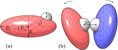
Figure 1: (a) Geometry of an ellipsoidal model particle with a reactive patch on its surface at some angle $\psi$ with respect to the symmetry axis $\mathbf{e}_{\parallel}$. (b) Illustration of an encounter configuration.

In order to study theoretically the effect of shape anisotropy on protein-protein encounter, we systematically vary the aspect ratio $\xi=R_{\parallel}/R_{\perp}$ of ellipsoids with a rotational symmetry, compare Fig. 1(a). This is one of the few systems for which closed analytic expressions of the translational (^t) and rotational (^r) friction coefficients $\zeta^{t/r}_{\parallel/\perp}(R_{\parallel},R_{\perp})$ are known Perrin (1934, 1936). Recently, the diffusional properties of such anisotropic particles have been investigated in great detail for two dimensions Han et al. (2006); Munk et al. (2009). Here we study three dimensions, both numerically and analytically. In addition, we not only consider anisotropy in diffusion, but also anisotropy in binding by placing spherical encounter patches at various positions on the ellipsoids. This approach allows us to assess in quantitative detail the relative role of hydrodynamic and steric anisotropy for protein-protein encounter.

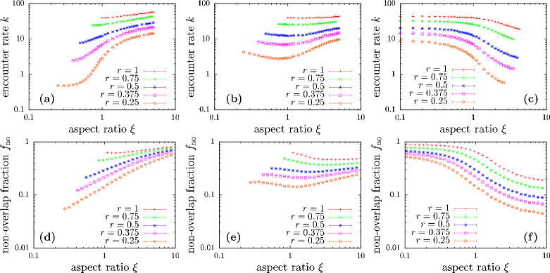
Figure 2: (a)–(c) Encounter rates for different patch sizes and locations. (d)–(f) Statistical estimate of the fraction of configuration space available for encounter. The patches are located according to $\mathcal{G}1$ in (a) and (d), $\mathcal{G}2$ in (b) and (e) and $\mathcal{G}3$ in (c) and (f).

To quantify the effect of anisotropy on molecular encounter, we performed Brownian dynamics simulations with a pair of ellipsoids in a periodic boundary box of edge length $L$, which represents the concentration of our system. The appropriate Langevin equation is evolved in discrete time steps $\Delta t$ via the Euler algorithm Schluttig et al. (2008):

$$\mathbf{X}(t+\Delta t)=\mathbf{X}(t)+\mathbf{g}(\Delta t)+\mathcal{O}(\Delta t^{2})\text{ .}$$ (1)

All vectors are six-dimensional generalized coordinates including the orientational information. The noise term $\mathbf{g}(\Delta t)$ is determined by the Einstein relation $\langle\mathbf{g}\rangle=\mathbf{0}$, $\langle\mathbf{g}(\Delta t)\cdot\mathbf{g}^{\dagger}(\Delta t)\rangle=2k_{B}T_{a}\mathbb{M}\Delta t$, where $T_{a}$ is ambient temperature and $\mathbb{M}=\mathbb{\zeta}^{-1}$ is the $6\times 6$ mobility matrix. In the following, all lengths are given in units of $U_{L}=R_{\perp}$ and times are scaled by $U_{T}=\zeta^{r}(R_{\perp},R_{\perp})/(k_{B}T_{a})$. In the simulations we chose $U_{L}=2\mathrm{nm}$ and thus $U_{T}\approx 50\mathrm{ns}$ at viscosity of water $\eta=1\mathrm{mPa\,s}$. As time step we use $\Delta t=2\cdot 10^{-5}$. We do not consider direct forces between the model particles in this study; in particular, we neglect electrostatic and two-body hydrodynamic interactions. Otherwise we implement hard-core repulsion. An analytic overlap criterion for a pair of ellipsoids is difficult to derive, but suitable algorithms based on the solution of the characteristic equation of the two ellipsoids have been derived for hard body fluids Allen et al. (1993).

Each of the model particles carries a spherical reactive patch of radius $r$ on its surface whose location is described by the angle $\psi$, compare Fig. 1(a). An overlap of these reactive patches is considered as an encounter, compare Fig. 1(b). We average over all initial conditions by starting $10^{4}$ simulations at random initial positions and orientations for each parameter set. The main quantity of interest is the encounter rate $k$, defined as the inverse first passage time to encounter. As it is common in Brownian dynamics of proteins, the encounter rate thus emerges from the definition of an absorbing boundary for the random walk Schreiber et al. (2009). For the two model particles in the simulation box we consider three scenarios of patch locations: $\psi_{1}=\psi_{2}=0$ ($\mathcal{G}1$); $\psi_{1}=0$, $\psi_{2}=\pi/2$ ($\mathcal{G}2$); $\psi_{1}=\psi_{2}=\pi/2$ ($\mathcal{G}3$).

In a coordinate system spanned by the principal axes, the friction matrix of an ellipsoid is diagonal. Taking the corresponding values for a sphere of radius $R_{\perp}$ as a reference scale, the diffusion coefficients $D^{t/r}_{\parallel/\perp}$ only depend on $\xi$. The relative translational mobility of an ellipsoid compared to a sphere is then given as $\lambda(\xi)=D^{t}_{\parallel}(\xi)+2D^{t}_{\perp}(\xi)$. According to the Smoluchowski equation, the encounter rate is expected to depend linearly on the mobility and the concentration of the reacting particles. Therefore we normalize the encounter rates obtained by our simulations by $\lambda(\xi)$ and by the volume of our simulation box (here $L^{3}=100^{3}$). The corresponding data is shown in Figs. 2(a)–(c). The rates are given in $1/U_{T}$. In each case, we exclude aspect ratios for which the reaction patches span the whole ellipsoid. Our simulation results show that encounter rates can vary up to two orders of magnitude depending on aspect ratio and patch position. While for patches located at the tips ($\mathcal{G}1$), encounter efficiency increases with aspect ratio, it decreases for patches located at the sides ($\mathcal{G}3$). For the mixed case ($\mathcal{G}2$), changes in aspect ratio have only a weak effect.

When interpreting these results, an important systematic difference between different aspect ratios $\xi$ has to be noted: As the geometry of the ellipsoid is changing with $\xi$, the exposed volume fraction $f_{V}$ of the reactive patches not covered by the steric particle is changing. We estimated the steric effect on the encounter rate by studying the fraction of non-overlapping ellipsoid configurations with touching reactive patches $f_{\mathrm{no}}$. A scheme of the setup is shown in Fig. 1(b). Particularly, the centers of the patches are placed at the distance $2r$ and both ellipsoids are randomly rotated around the center of their respective patch. The results for $f_{\mathrm{no}}$ from drawing $10^{5}$ of such random encounter configurations are shown in Figs. 2(d)–(f) for the parameters corresponding to Figs. 2(a)–(c). The plots show that the qualitative features of the encounter rates are well reproduced by the steric constraints. This leads to the conclusion that the main reason for the changes in the encounter rate in the preceeding study is not the altered hydrodynamic behavior of the ellipsoids but the steric hindering of encounters due to the changing geometry.

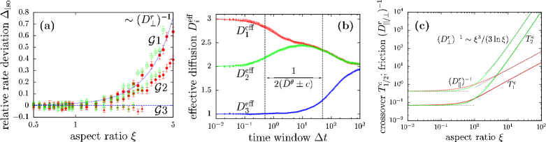
Figure 3: (a) Relative deviation of the encounter rates from the original data (compare Fig. 2) assuming isotropic motion at all times. Reactive patches have a radius of $r=0.5$. The dotted line indicates the supposed scaling and the dashed line marks $\Delta_{\mathrm{iso}}=0$. Data from simulations with $L=100$ is shown with red, filled symbols, data with $L=20$ is shown with green, hollow symbols. (b) Example of the time window dependency of the effective principal translational diffusion coefficients for the following choice of parameters (generic units): $D_{1}=3$, $D_{2}=2$, $D_{3}=1$, $D^{\theta}_{1}=0$, $D^{\theta}_{2}=0.005$, $D^{\theta}_{3}=0.5$. The data points have been obtained by simulation (the error bars depict the standard deviation obtained from $10^{5}$ individual runs), the solid lines represent the theoretic prediction and the dashed lines indicate the two relevant time scales for the crossover as given in Eq. (8). (c) Crossover times and rotational friction coefficients for ellipsoids for a wide range of aspect ratios.

To obtain another measure for the effect of hydrodynamics, we compared our simulations with explicit anisotropic diffusion to simulations, where we do not account for the anisotropy in the diffusion matrix. Particularly, we use an isotropic diffusion matrix with the average translational and rotational diffusion coefficients $D^{t}_{\mathrm{avg}}=(D^{t}_{\parallel}+2D^{t}_{\perp})/3$, which is equal to the isotropic limit, and $D^{r}_{\mathrm{avg}}=(D^{r}_{\parallel}+2D^{r}_{\perp})/3$, respectively. We perform the same simulations as in Fig. 2 with this new $\mathbb{D}$. Moreover, we compared to simulations at higher effective concentration ($L=20$). Fig. 3 shows the relative deviation of the encounter rates $\Delta_{\mathrm{iso}}=k_{\mathrm{isotropic}}/k_{\mathrm{anisotropic}}-1$. Interestingly, in case $\mathcal{G}3$ there is no significant deviation from the original results. However, considering $\mathcal{G}1$ the (artificial) isotropic encounter rate is larger for prolates ($\xi>1$). This effect can also be observed in the mixed case $\mathcal{G}2$, decreased by roughly a factor $2$. This is reasonable as here only one of the two encountering ellipsoids has its patch at $\psi=0$. These findings show that the anisotropic diffusion of elongated ellipsoids leads to a decrease of the encounter rates. However, the deviation up to $\xi=5$ is moderate ($\Delta_{\mathrm{iso}}\approx 0.7$), so we conclude that the impact of anisotropic diffusion on molecular encounter is rather weak.

Anisotropic diffusion in isotropic environments is only relevant on small time and length scales. In the following, we derive the effective translational diffusion properties for a finite time window $\Delta t$ considering an arbitrary body with three different translational ($D_{i}$) and rotational ($D^{\theta}_{i}$) diffusion coefficients along the principal axis (in the body-fixed coordinate system). As the rotations due to rotational diffusion are supposed to be completely independent, the crossover only affects the effective translational diffusion which is described by a $3\times 3$ diffusion matrix: $\mathbb{D}^{t}_{ij}=\delta_{ij}D_{i}$, where $\delta_{ij}$ is the Kronecker delta. A rotation determined by a vector of angles $\bm{\theta}=(\theta_{1},\theta_{2},\theta_{3})^{\dagger}$ around the three principal axes can be described by the rotation matrix $\mathbb{S}=e^{-\bm{\theta}\cdot\mathbf{J}}$, with $\mathbf{J}=\left(\mathbb{J}^{1}\text{, }\mathbb{J}^{2}\text{, }\mathbb{J}^{3}\right)^{\dagger}$. $\bm{\theta}\cdot\mathbf{J}$ denotes a formal scalar product and $\mathbb{J}^{k}$ are matrices defined by $\mathbb{J}^{k}_{ij}=\epsilon_{ikj}$, where $\epsilon$ is the Levi-Civita symbol. We proceed considering only small rotations occurring at small times, so that we can expand the rotation in orders of $\theta$:

$$\mathbb{S}_{ij}=\delta_{ij}\frac{2-\bm{\theta}^{2}}{2}+\epsilon_{ikj}\theta_{k}\frac{6-\bm{\theta}^{2}}{6}+\frac{\theta_{i}\theta_{j}}{2}+\mathcal{O}(\theta^{4})\text{ ,}$$ (2)

where $\bm{\theta}^{2}=\sum_{i=1}^{3}\theta_{i}^{2}$. This rotation is applied to $\mathbb{D}^{t}$ and we get $\bar{\mathbb{D}^{t}}=\mathbb{S}\mathbb{D}^{t}\mathbb{S}^{\mathsf{T}}$, where we will only consider terms up to second order in $\theta$ in the following. Furthermore we average over all possible orientations, weighted by the probability density $p(\theta_{i},t)\sim\exp(-\theta_{i}^{2}/(4D^{\theta}_{i}t))$ due to rotational diffusion. As we consider only small $\theta$ and $t\ll 1$, it will now also be sufficient to expand $p(\theta_{i},t)$ up to second order in $t$. Hence, the Gaussian probability distribution can be replaced by a uniform distribution regarding correct integral boundaries. The non-diagonal entries are odd in $\theta_{i}$ and thus vanish. The average of the diagonal entries is the central quantity for the calculation of the mean square displacement:

$$\langle\bar{\mathbb{D}^{t}}_{ii}\rangle_{t} =\frac{1}{w_{1}w_{2}w_{3}}\int\limits_{-w_{1}/2}^{w_{1}/2}\text{d}\theta_{1}\int\limits_{-w_{2}/2}^{w_{2}/2}\text{d}\theta_{2}\int\limits_{-w_{3}/2}^{w_{3}/2}\text{d}\theta_{3}\bar{\mathbb{D}^{t}}_{ii}\text{ ,}$$ (3)

where $w_{i}=\sqrt{24D^{\theta}_{i}t}$ is the width of the uniform distribution interval. Only terms of even orders of $\theta_{i}$ will contribute. That is, the integral in Eq. 3 will only lead to zeroth and second moments of the angular distribution. By the average action of the rotational diffusion, $D_{i}$ transforms into an effective translational diffusion constant $\langle\bar{\mathbb{D}^{t}}_{ii}\rangle_{t}$ over time $t$ in the fixed laboratory coordinate space. Considering a vector $\mathbf{D}=(D_{1},D_{2},D_{3})$, the evolution of the effective, orientation averaged vector of diffusion coefficients $\langle\mathbf{D}\rangle(t)=(\langle\bar{\mathbb{D}^{t}}_{11}\rangle_{t},\langle\bar{\mathbb{D}^{t}}_{22}\rangle_{t},\langle\bar{\mathbb{D}^{t}}_{33}\rangle_{t})$ can be expressed in a matrix form, not taking into account non-linear terms in $t$:

$$\langle\mathbf{D}\rangle(t) =\mathbf{D}\cdot\mathbb{R}(t)+\mathcal{O}(t^{2})\text{ ,}$$ (4)

$$\mathbb{R}_{ij}(t) =2t|\epsilon_{ijk}|D^{\theta}_{k}+\delta_{ij}(1+2t(D^{\theta}_{i}-\bar{D^{\theta}}))\text{ ,}$$ (5)

where $\bar{D^{\theta}}=\sum_{k=1}^{3}D^{\theta}_{k}$. The principal axes of effective motion are constant since the coupling terms between the translational degrees of freedom vanish when averaging over all possible orientations. Because rotational diffusion is independent of time and orientation, $\mathbb{R}$ keeps its form for all times. We can also apply $\mathbb{R}(\delta t)$ to some diffusion vector $\langle\mathbf{D}\rangle(t)$. Thus, it is possible to evaluate the effective change of the diffusion coefficients for large times $t$ in small steps $\delta t=t/N$ with only making errors of $\mathcal{O}(N\delta t^{2})$:

$$\langle\mathbf{D}\rangle(N\delta t) =\mathbf{D}\cdot\left(\mathbb{R}(\delta t)\right)^{N}+\mathcal{O}(N\delta t^{2})\text{ .}$$ (6)

In the limit of large $N$ the error in Eq. (6) vanishes: $\mathcal{O}(Nt^{2}/N^{2})=\mathcal{O}(t^{2}/N)\rightarrow 0$. This basically means that we calculate $\langle\mathbf{D}\rangle(t)$ with infinite accuracy. We can now evaluate the overall, orientation averaged mean square displacement by integrating $\langle\mathbf{D}\rangle(t)$ with respect to $t$:

$$\langle\mathbf{x}(t)^{2}\rangle =\begin{pmatrix}2ft+(ad_{2}-bd_{3})g_{-}+cd_{1}g_{+}\\ 2ft+(ad_{1}-bd_{2})g_{-}+cd_{2}g_{+}\\ 2ft+(ad_{3}-bd_{1})g_{-}+cd_{3}g_{+}\end{pmatrix}\text{ ,}$$ (7)

with $a=D^{\theta}_{3}-D^{\theta}_{1}$, $b=D^{\theta}_{1}-D^{\theta}_{2}$, $c=\sqrt{a^{2}+b^{2}+ab}$, $d_{i}=3(D_{i}-f)$, $f=\sum_{i=1}^{3}D_{i}/3$, and

$$g_{\pm} =\dfrac{1-e^{-2(\bar{D^{\theta}}-c)t}}{6(\bar{D^{\theta}}-c)c}\pm\dfrac{1-e^{-2(\bar{D^{\theta}}+c)t}}{6(\bar{D^{\theta}}+c)c}\text{ .}$$ (8)

This result can be used to obtain effective translational diffusion coefficients via $\mathbf{D}^{\mathrm{eff}}(\Delta t)=\langle\mathbf{x}^{2}(\Delta t)\rangle/2t$, compare Fig. 3(b). Thus, the crossover from anisotropic to isotropic diffusion in 3D occurs on two time scales $T^{c}_{1/2}=1/(2\bar{D^{\theta}\pm c})$ which increasingly deviate with increasing anisotropy.

The corresponding crossover times for ellipsoids are $T^{c}_{1}=1/(4D^{r}_{\parallel}(\xi)+2D^{r}_{\perp}(\xi))$ and $T^{c}_{2}=1/(6D^{r}_{\perp}(\xi))$. The rotational friction coefficients and their implication for $T^{c}_{1/2}$ are shown in Fig. 3(c). The asymptotic behavior indicated in the plot can be derived from the full solution of the friction coefficients. For $\xi<0$ both $D^{r}_{\parallel}$ and $D^{r}_{\perp}$ approach a constant value. Therefore, regarding rotational diffusion no significant differences are expected for oblates, which corresponds well to the findings from Fig. 3(a). In contrast, rotational diffusion particularly around $\mathbf{e}_{\perp}$, which governs $T^{c}_{2}$, is strongly decreased for large $\xi$. Therefore, the relevant range of anisotropic diffusion grows and the indication of the scaling in Fig. 3(a) shows that this again corresponds well to the simulation data. Assuming this scaling to govern the impact of hydrodynamic anisotropy, one might argue that the effect will be strongest for $\xi\gg 1$ and small $L$, i.e. large concentrations. However, if we require $L>2\xi$, so that the particles fit into the simulation box, encounter times are larger than $T^{c}_{2}$ for all values of $\xi$. Thus our analytical calculation confirms that anisotropic diffusion does not have a strong effect on protein-protein encounter rates. This finding also validates computational schemes which assume isotropic diffusion for efficient description of the diffusion steps van Zon and ten Wolde (2005).

An interesting question that has not been addressed yet is whether the effect of hydrodynamic anisotropy is stronger regarding re-encounter. Dynamic dissociation and re-association can be easily realized in our model for example by introducing a finite average lifetime for each bond. Recently it has been shown with a similar Brownian dynamics approach that productive protein-protein encounter is preceded by many non-productive contacts Schluttig et al. (2008). In a similar vein, dissociation after binding is likely to be followed by additional encounters. Because prolates have a lower overall rotational diffusion coefficient, one expects that they are more likely to return to an encounter. It might well be that for re-encounter, the aspect ratio plays a more important role for accessibility of the binding site than found here for protein diffusion to the first encounter. Similar considerations might be valid for protein dynamics in the context of protein clusters, where diffusion might be restricted by the presence of other components.

References

- Schreiber et al. (2009) G. Schreiber, G. Haran, and H. X. Zhou, Chem. Rev. 109, 839 (2009).
- Ermak and McCammon (1978) D. L. Ermak and J. A. McCammon, J. Chem. Phys. 69, 1352 (1978).
- Northrup and Erickson (1992) S. Northrup and H. Erickson, Proc. Natl. Acad. Sci. USA 89, 3338 (1992).
- van Zon and ten Wolde (2005) J. S. van Zon and P. R. ten Wolde, Phys. Rev. Lett. 94, 128103 (2005).
- de la Torre et al. (2000) J. G. de la Torre, M. L. Huertas, and B. Carrasco, Biophys. J. 78, 719 (2000).
- Gabdoulline and Wade (1997) R. R. Gabdoulline and R. C. Wade, Biophys. J. 72, 1917 (1997).
- Perrin (1934) F. Perrin, J. Phys. Radium 5, 497 (1934).
- Perrin (1936) F. Perrin, J. Phys. Radium 7, 1 (1936).
- Han et al. (2006) Y. Han, A. M. Alsayed, M. Nobili, J. Zhang, T. C. Lubensky, and A. G. Yodh, Science 314, 626 (2006).
- Munk et al. (2009) T. Munk, F. Hofling, E. Frey, and T. Franosch, Eur. Phys. Lett. 85, 30003+ (2009).
- Schluttig et al. (2008) J. Schluttig, D. Alamanova, V. Helms, and U. S. Schwarz, J. Chem. Phys. 129, 155106 (2008).
- Allen et al. (1993) M. Allen, G. Evans, D. Frenkel, and B. Mulder, Adv. Chem. Phys. 86, 1 (1993).