Thick gas discs in faint dwarf galaxies

Abstract

We determine the intrinsic axial ratio distribution of the gas discs of extremely faint M${}_{B}>-14.5$ dwarf irregular galaxies. We start with the measured (beam corrected) distribution of apparent axial ratios in the HI 21cm images of dwarf irregular galaxies observed as part of the Faint Irregular Galaxy GMRT Survey (FIGGS). Assuming that the discs can be approximated as oblate spheroids, the intrinsic axial ratio distribution can be obtained from the observed apparent axial ratio distribution. We use a couple of methods to do this, and our final results are based on using Lucy’s deconvolution algorithm. This method is constrained to produce physically plausible distributions, and also has the added advantage of allowing for observational errors to be accounted for. While one might a priori expect that gas discs would be thin (because collisions between gas clouds would cause them to quickly settle down to a thin disc), we find that the HI discs of faint dwarf irregulars are quite thick, with mean axial ratio $<q>\sim 0.6$. While this is substantially larger than the typical value of $\sim 0.2$ for the stellar discs of large spiral galaxies, it is consistent with the much larger ratio of velocity dispersion to rotational velocity ($\sigma/v_{c}$) in dwarf galaxy HI discs as compared to that in spiral galaxies. Our findings have implications for studies of the mass distribution and the Tully - Fisher relation for faint dwarf irregular galaxies, where it is often assumed that the gas is in a thin disc.

1 Introduction

The intrinsic shape of galaxies is interesting from a variety of perspectives. For a given galaxy the shape should be consistent with the dynamical model of the galaxy, while, for a sample of galaxies, one would expect that a correct evolutionary model should be able to reproduce the observed distribution of shapes. It is generally assumed that disc galaxies can be approximated to be oblate spheroids (e.g. Hubble (1926); Sandage, Freeman, & Stokes (1970); Ryden (2006)). If one further assumes that the galaxies have a well defined mean axial ratio (q₀), then the observed axial ratio can be used to determine the inclination of the disc. In turn, the inclination is a crucial input in dynamical modeling (e.g. for the mass and structure of the dark matter halo), studying the Tully-Fisher relation etc.

The observed shape of a galaxy differs from the intrinsic shape because of projection effects. If one has a sample of galaxies drawn from a population with a well defined intrinsic axial ratio distribution and with random orientations with respect to the earth, then one can determine the distribution of intrinsic axial ratios from the observed axial ratio distribution (for e.g.  Noerdlinger, 1979; Binney & de Vaucouleurs, 1981; Lambas, Maddox & Loveday, 1992; Ryden, 2006). It is worth noting that most of these studies have focused on large galaxies, and that there have been relatively few that focused on dwarfs. For bright spiral galaxies, q₀ is often taken to be $\sim 0.2$ (see e.g.  Haynes & Giovanelli, 1984; Verheijen & Sancisi, 2001). It has also long been appreciated that the axial ratio is a function of Hubble type. For example, Heidmann, Heidmann, & de Vaucouleurs (1972) found that while discs get thinner as one goes from galaxies of morphological type Sa to Sd, there is a rapid increase in disc thickness as one goes from Sd to dwarf Irregular galaxies. Similarly, Staveley-Smith, Davies & Kinman (1992) found that dwarf galaxies from the UGC catalog have q${}_{0}\sim 0.5$. Axial ratio is also a function of the wavelength of observation. For example, Ryden (2006) showed that older populations as traced by redder stars have thicker ratios than the corresponding B band disc. But all of these studies refer to the stellar discs of the galaxies. Due to collisions between gas clouds, one would expect that the gas discs would be intrinsically quite thin, for example, for our Galaxy, the scale height of the middle disc is only $\sim 300$ pc. In extremely gas rich dwarf galaxies one might then expect that the gas discs are relatively thin, even though the stellar disc may have a large axial ratio.

We present here a study of the axial ratio distribution of the HI discs of extremely faint dwarf irregular galaxies. We select a sample of galaxies for which HI synthesis observations are available from the Faint Irregular Galaxy GMRT Survey (FIGGS, Begum et al. (2008)). The sample selection and analysis methods used are presented in section 2, while the results are discussed in section 3. To the best of our knowledge, this is the first such study of the intrinsic shape of the HI discs of galaxies.

2 Sample Selection, Analysis and Results

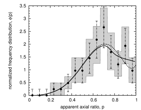
Figure 1: Histograms of the measured apparent axial ratios (after correction for the finite beam size). There are a total of 15 bins, the error bars were determined assuming Poisson statistics. The shaded area represents the 80% confidence limit histograms generated by bootstrap re-sampling of the data (see text for details). The dashed line shows the best fit (i.e. using the weighted least square) polynomial to the binned data. The solid black line is the reconstructed distribution ($\Phi(p)$) given by Lucy deconvolution (see text for details). All values have been normalized so that the area under the curves and histogram is unity.

The FIGGS sample was selected to satisfy the following criteria: (1) absolute blue magnitude M${}_{\rm B}>-14.5$, (2) integrated HI flux $>1$ Jy km/s and (3) optical major axis $>1^{{}^{\prime}}$. There are total of 62 galaxies in the FIGGS sample, for all of which we have axis ratios available. We discuss the implications of the selection criteria on our derived axis ratio in Sec. 3; here we merely note that any bias in the sample is likely to be towards having a preference for edge on systems. The FIGGS survey presents HI images at a range of angular resolutions. Since we are interested in the overall shape of the disc, we measured the axis ratio of the disc using the coarsest resolution HI maps. This was done because we wanted to avoid the fine structure which shows up at higher resolutions, and instead trace the complete spatial spread of HI which requires observing the less dense gas using coarser resolution. For all of these galaxies, elliptical isophotes were fit to the HI image using the STSDAS package in IRAF. The axis ratio that we use in this paper was measured for the isophote with mean column density $10^{19}$ cm^-2 for all galaxies. The measured axial ratio was corrected for the finite beam size before being used.

For a sample of randomly oriented axi-symmetric oblate spheroids, with intrinsic axial ratio distribution $\psi(q)$, where the axial ratio $q$ is defined as $q=c/a$, with $c$ being the short axis (“thickness”) of the spheroid and $a$ the long axis (“diameter”), the observed distribution of axis ratios $\phi(p)$, where $p$ is the observed axial ratio is given by (see e.g. Binney (1978))

$${\phi(p)~{}=~{}p{\displaystyle\int_{0}^{p}}{\frac{\psi(q)dq}{\sqrt{(1-q^{2})(p^{2}-q^{2})}}}}$$ (1)

What is available to us is $\phi(p)$  the observed axial ratio distribution; in order to derive the intrinsic axial ratio distribution $\psi(q)$ , we have to invert Eqn. 1.

Fall & Frenk (1983) provide an integration formula (Eqn. (7) in their paper) in the case that $\phi(p)$  is a polynomial function. This allows for a direct inversion of Eqn. 1. The binned data (Fig. 1) were hence fit by a polynomial, using a weighted least squares fit. The errors were assumed to be Poisson distributed (with the error for bins with zero counts taken to be that for a single count). The errors were also estimated using bootstrap resampling. 10000 different realizations of the data were constructed using boot strap resampling, and the 80% confidence limit histograms determined in this way are also shown in Fig. 1. As can be seen, the two error estimates are in good agreement. The direct inversion of the best fit polynomial is shown in Fig. 2. It has a broad peak around q${}_{0}\sim 0.6$, but also falls to negative values beyond $q~{}\sim~{}0.8$, which is unphysical.

While there may exist an acceptable polynomial fit to $\phi(p)$  which does not produce negatives on inversion, we do not investigate this possibility directly. Instead we choose to try to invert Eqn. 1 using Lucy’s deconvolution algorithm (Lucy, 1974). This approach has the added advantage of also being able to account for measurement errors. The Lucy deconvolution method is an iterative algorithm for estimating the intrinsic frequency distribution from an observed distribution, subject to the constraints that the deduced distribution should be normalized as well as positive for all values of the intrinsic quantity ($q$ in our case). One starts with an initial guess initial guess for the intrinsic distribution ($\psi(q)$), and uses a kernel ($k(p|q)$, defined by Eqn. 2 below) to iteratively find better approximations to both the apparent distribution and the intrinsic distribution.

If we rewrite Eqn. 1 as:

$$\phi(p)={\displaystyle\int}\psi(q)k(p|q)dq$$ (2)

then the $r$th loop of the iterative algorithm will be,

$$\Phi^{r}(p)~{}=~{}{\displaystyle\int}\psi^{r}(q)k(p|q)dq$$ (3)

$$\psi^{r+1}(q)~{}=~{}\psi^{r}(q){\displaystyle\int}{\frac{\phi(p)}{\Phi^{r}(p)}}k(p|q)dp$$ (4)

Eqn. 4 neglects the measurement errors in determining the observed axial ratio. Following Binney & de Vaucouleurs (1981), we can account for these errors by assuming the following form for the probability $E(p|p^{\prime})\delta p$, that a galaxy of actual apparent axial ratio $p^{\prime}$ is instead measured to have an axial ratio $p$:

$$E(p|p^{\prime})={\frac{1}{\sqrt{2\pi}\sigma}}[\exp({\frac{-(p-p^{\prime})^{2}}{2\sigma^{2}}})+\exp({\frac{-(2-(p+p^{\prime}))^{2}}{2\sigma^{2}}})]$$ (5)

In our case, we estimate the measurement errors by fitting a straight line to the distribution of errors in the axial ratio $p$ as reported by the isophote fitting package. This gives:

$$\sigma(p^{\prime})~{}=~{}0.029p^{\prime}~{}+~{}0.0006$$ (6)

and projection kernel hence becomes,

$$K(p|q)={\displaystyle\int_{q}^{1}}E(p|p^{\prime})k(p^{\prime}|q)dp^{\prime}$$ (7)

The algorithm now involves using $K(p|q)$ instead of $k(p|q)$ in equations 3 and 4, for which the range of integration now becomes 0 to 1, since now $K(p|q)\not=0$ for $p<q$. One would expect that in successive iterations, the approximation $\Phi(p)$ to the observed distribution $\phi(p)$  improve, and this can be used to decide when to terminate the algorithm.

Two different initial guesses for $\psi(q)$ ($\psi^{0}(q)$) were tried, the first was peaked around $q\sim 0.6$, the second was constant for all $q$. These two initial guesses thus cover two extremes of possible $\psi(q)$. For both initial guesses, $\psi(q)$  quickly converges to the form shown in Fig. 2. To determine the indicative errors in the determination of $\psi(q)$ , the 80% confidence limit histograms shown in Fig. 1 were fit with polynomials and Lucy deconvolution was applied to these polynomials. The resulting intrinsic distribution functions are also shown in Fig. 2, and the shaded area hence represents the $\sim$ 80% confidence interval for $\psi(q)$. The final $\Phi(p)$ (i.e. the final approximation to the observed distribution function) is shown in Fig. 1, and as it can be seen, it fits with the observed distribution within the error bars. The $\psi(q)$  shown in Fig. 2 has $<q>~{}=~{}0.57$, standard deviation $\sigma~{}=~{}0.164$, and skewness, $\gamma_{1}~{}=~{}q^{3}/\sigma^{3}~{}=~{}-0.62$.

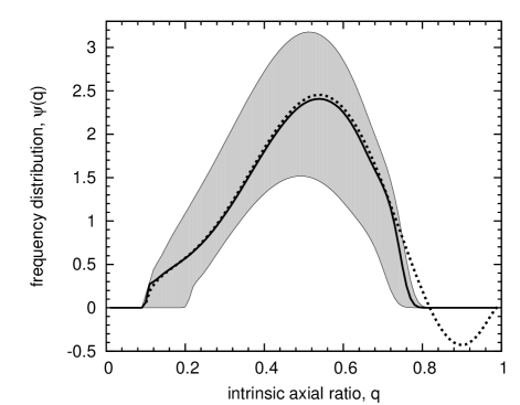
Figure 2: The frequency distribution of intrinsic axial ratios. The dashed line indicates $\psi(q)$  as obtained from the direct inversion of the polynomial fit to the binned data. The solid line is the final $\psi(q)$  obtained after Lucy deconvolution (see text for details). The shaded area represents the region between the $\psi(q)$s obtained by applying Lucy deconvolution to the polynomial fits to the 80% confidence interval histograms (see text for details).

3 Discussion

Eqn. 1 (and hence results obtained from inverting it also) applies only for a sample of randomly oriented oblate spheroids. The basic assumption hence is that the galaxy sample we are working with has an unbiased distribution of inclination angles. The selection criteria for the FIGGS sample (from which the current sample is drawn) includes a requirement that the optical major axis of the galaxy be $>1^{{}^{\prime}}$. Dwarf galaxies are generally dust poor (for eg. see Walter et al., 2007; Galametz et al., 2009), and hence to a good approximation have optically thin discs. Highly inclined galaxies will hence be over represented in a diameter limited sample, i.e. our sample is biased towards edge on discs. This means that the true mean intrinsic axial ratio would be even larger than what we have estimated above. It is worth noting that as the intrinsic axial ratio gets closer to 1.0, the magnitude of this bias decreases, and hence the bias in our estimate should not be large.

The mean intrinsic axial ratio that we obtain, viz. $<q>\sim 0.57$ is substantially larger than the value of $0.2$ usually adopted for the stellar discs of large spiral galaxies. The value from our sample is more than twice as large as older measurements of $<q>$ in stellar discs of Magellanic irregular galaxies by Heidmann, Heidmann, & de Vaucouleurs (1972) (ranging from 0.20 to 0.24). Consistent with this, our sample contains no very flat galaxies. In fact, as can be seen from Fig. 1 there are no galaxies with apparent axial ratio $<0.2$ in the sample. Further, if we look at the distribution of the observed axial ratio of different classes of galaxies in the Automated Photographic Measuring (APM) survey as in Lambas, Maddox & Loveday (1992), then our histogram resembles those for ellipticals and S0s more closely than that for spirals. This is another qualitative indication that the underlying intrinsic distribution of axial ratios has a higher mean than is typical for spirals. Interestingly, the value of $<q>$ we obtain matches well with what Staveley-Smith, Davies & Kinman (1992); Binggeli & Popescu (1995) derived for the stellar discs in dwarfs.

The thickness of the gas discs of dwarf galaxies is contrary to what one might have naively expected for a gas disc, since, in general, collisions between gas clouds should cause them to quickly settle into a thin disc. However, this large axial ratio is probably consistent with the large gas dispersion in comparison to the rotational velocity observed in dwarf galaxies. For example, Kaufmann, Wheeler and Bullock (2007) did particle hydrodynamic simulations to show that dwarf galaxies with rotational velocities $\sim$40 km s^-1 did not originate as thin discs but thick systems. This still leaves open the question of where the large velocity dispersion comes from. Dutta et al. (2009) find good evidence for a scale free power spectrum of HI fluctuations in dwarf galaxies, consisent with what would be expected from a turbulent medium. Interestingly, they also find that that the dwarfs must have relatively thick gas discs, similar to the conclusions reached here. Assuming that the origin of the velocity dispersion is turbulent motions in the ISM, the timescale for dissipation is given by $\tau\sim L/v_{turb}\sim L/\sigma$ (Shu, Adams, & Lizano, 1987, e.g.). The total turbulent energy is $E_{turb}\sim 1/2M_{HI}\sigma^{2}$. For our sample galaxies, the typical HI mass is $\sim 3\times 10^{7}$ M_⊙, while the length scale $L\sim 1$kpc. The rate of turbulent energy dissipation is hence $\sim 10^{44}$erg/yr. On the other hand, the star formation rate is $\sim 10^{-3}$ M_⊙/yr (Roychowdhury et al., 2009), for which the expected supernova rate for a Salpeter IMF is $\sim 7\times 10^{-6}$/yr (Binney, 2001). Assuming that each supernova explosion deposits $\sim 10^{51}$ ergs of energy into the ISM, the energy input from star formation is $\sim 10^{46}$ ergs/yr, more than sufficient to balance the turbulent energy loss. Thus, star formation driven turbulence in the ISM is a plausible cause for the thick gas discs that we observe.

We have assumed through out that the HI discs of dwarf galaxies can be approximated as oblate spheroids. On the other hand, in Sec. 2 we saw that the inversion based on the best fit polynomial to the observed histogram of axial ratios actually gives unphysical results, i.e. that the derived intrinsic axial ratio distribution $\psi(q)$ becomes negative. Lambas, Maddox & Loveday (1992) found a similar pattern for the axial ratio distribution of spiral and S0 galaxies in the APM catalog, and hence relaxed the assumption that the discs are oblate spheroids. Adequate fits to their data could be obtained assuming that the galaxies have a triaxial shape. Similarly, Ryden (2006) from a study of large galaxies in the 2MASS catalog concluded that spiral galaxies are mildly triaxial. The fact that the polynomial approximation gives unphysical results for our sample also suggests that triaxial models may provide a better fit. On the other hand, the Lucy deconvolution gives a physically plausible (as indeed it is designed to) intrinsic axial ratio distribution, that fits the observed data within the error bars. It is worth noting that distribution found by Lucy deconvolution is in excellent agreement with that found by direct inversion of the polynomial fit for the entire range for which the latter is $>0$. Interestingly, if we assume the gas discs to be prolate instead of oblate spheroids, Lucy deconvolution produces an equally acceptable $\phi(p)$  as can be seen from Fig. 3. The $\psi(q)$  obtained from Lucy deconvolution with a prolate spheroid assumption (see Fig. 4) indicates that such gas discs should be more cylindrical than spherical. However, the observed kinematics of gas in these galaxies (see Begum et al., 2003; Begum & Chengalur, 2003, 2004a, 2004b; Begum, Chengalur & Karachentsev, 2005; Begum et al., 2005, 2006, 2008, etc.) shows that the gas has a significant rotational support. As discussed earlier, a gravitationally bound rotating disc of gas forms an oblate and not a prolate spheroid. Thus, although from the axial ratio data alone, one cannot distinguish between a prolate and oblate shapes, in conjuction with the kinematical data, it is clear that the gas is distributed in the form of a thick disc.

Figure 3: Reconstructed axial ratio distribution ($\Phi(p)$) assuming the gas discs to be prolate spheroids, is shown as boxes, which follows the best fit polynomial to the binned data (solid line) closely. Binned data with errorbars and the reconstructed distribution $\Phi(p)$ obtained using the oblate spheroid assumption (dashed line) is shown for comparison. All values have been normalized to unity.

Figure 4: The frequency distribution of intrinsic axial ratios obtained after Lucy deconvolution. The dashed line indicates $\psi(q)$  obtained assuming the gas discs to be prolate spheroids, while the solid line shows the earlier $\psi(q)$  obtained with the oblate spheroid assumption.

In summary, we find that the gas discs of dwarf galaxies are relatively thick, in sharp contrast to the gas discs of spiral galaxies. This has implications both for the internal dynamics of the gas, as well as for studies of the mass distribution Tully - Fisher relation in faint dwarfs, in which it is generally assumed that the gas is in a thin disc.

References

- Begum et al. (2003) Begum, A., Chengalur, J.N. & Hopp, U., 2003, New Astronomy, 8, 267
- Begum & Chengalur (2003) Begum, A & Chengalur, J.N., 2003, A&A, 409, 879
- Begum & Chengalur (2004a) Begum, A & Chengalur, J.N., 2004, A&A, 413, 525
- Begum & Chengalur (2004b) Begum, A & Chengalur, J.N., 2004, A&A, 424, 509
- Begum, Chengalur & Karachentsev (2005) Begum, A, Chengalur, J.N. & Karachentsev, I. D., 2005, A&A, 433, 1L
- Begum et al. (2005) Begum, A, Chengalur, J.N., Karachentsev, I. D. & Sharina, M. E., 2005, MNRAS, 359, 53L
- Begum et al. (2006) Begum A., Chengalur J. N., Karachentsev I. D., Kaisin S. S. & Sharina M. E., 2006, MNRAS, 365,1220
- Begum et al. (2008) Begum A., Chengalur J. N., Karachentsev I. D., Sharina M. E. & Kaisin S. S., 2008, MNRAS, 386, 1667B
- Binggeli & Popescu (1995) Binggeli B., Popescu C. C., 1995, A&A, 298, 63
- Binney (2001) Binney J., 2001, in Hibbard J. E., Rupen M. P., von Gorkom H., eds, ASP Conf. Ser. Vol. 240, Gas and Galaxy Evolution, Astron. Soc. Pac., San Francisco, p. 355
- Binney (1978) Binney J., 1978, MNRAS, 183, 501
- Binney & de Vaucouleurs (1981) Binney J. & de Vaucouleurs G., 1981, MNRAS, 194, 679
- Dutta et al. (2009) Dutta Prasun, Begum Ayesha, Bharadwaj Somnath, & Chengalur Jayaram N., 2009, MNRAS, 398, 887
- Fall & Frenk (1983) Fall S. M. & Frenk C. S., 1983, AJ, 88(11), 1626
- Galametz et al. (2009) Galametz M., et al., 2009, A&A, 508, 645
- Haynes & Giovanelli (1984) Haynes M. P., Giovanelli R., 1984, AJ, 89, 758
- Heidmann, Heidmann, & de Vaucouleurs (1972) Heidmann J., Heidmann N., de Vaucouleurs G., 1972, Mem. Roy. Astron. Soc., 75, 85
- Hubble (1926) Hubble E. P., 1926, ApJ, 64, 321
- Kaufmann, Wheeler and Bullock (2007) Kaufmann T., Wheeler C., Bullock J. S., 2007, MNRAS, 382, 1187
- Lambas, Maddox & Loveday (1992) Lambas D. G., Maddox S. J. & Loveday J., 1992, MNRAS, 258,404
- Lucy (1974) Lucy L. B., 1974, AJ, 79(6), 745
- Noerdlinger (1979) Noerdlinger Peter D., 1979, ApJ, 234, 802
- Roychowdhury et al. (2009) Roychowdhury S., Chengalur J. N., Begum A., Karachentsev I. D., 2009, MNRAS, 397, 1435
- Ryden (2006) Ryden B. S., 2006, ApJ, 641, 773
- Sandage, Freeman, & Stokes (1970) Sandage A., Freeman K. C., Stokes N. R., 1970, ApJ, 160, 831
- Shu, Adams, & Lizano (1987) Shu F. H., Adams F. C., Lizano S., 1987, ARA&A, 25, 23
- Staveley-Smith, Davies & Kinman (1992) Staveley-Smith L., Davies R. D. & Kinman T.D., 1992, MNRAS, 258, 334
- Verheijen & Sancisi (2001) Verheijen M. A. W., Sancisi R., 2001, A&A, 370, 765
- Walter et al. (2007) Walter Fabian et al., 2007, ApJ, 661, 102