Deterministic Sample Sort For GPUs

Abstract

We present and evaluate GPU Bucket Sort, a parallel deterministic sample sort algorithm for many-core GPUs. Our method is considerably faster than Thrust Merge (Satish et.al., Proc. IPDPS 2009), the best comparison-based sorting algorithm for GPUs, and it is as fast as the new randomized sample sort for GPUs by Leischner et.al. (to appear in Proc. IPDPS 2010). Our deterministic sample sort has the advantage that bucket sizes are guaranteed and therefore its running time does not have the input data dependent fluctuations that can occur for randomized sample sort.

1 Introduction

Modern graphics processors (GPUs) have evolved into highly parallel and fully programmable architectures. Current many-core GPUs such as nVIDIA’s GTX and Tesla GPUs can contain up to 240 processor cores on one chip and can have an astounding peak performance of up to 1 TFLOP. The upcoming Fermi GPU recently announced by nVIDIA is expected to have more than 500 processor cores. However, GPUs are known to be hard to program and current general purpose (i.e. non-graphics) GPU applications concentrate typically on problems that can be solved using fixed and/or regular data access patterns such as image processing, linear algebra, physics simulation, signal processing and scientific computing (see e.g. [7]). The design of efficient GPU methods for discrete and combinatorial problems with data dependent memory access patterns is still in its infancy. In fact, there is currently still a lively debate even on the best sorting method for GPUs (e.g. [14, 9]).

Until very recently, the comparison-based Thrust Merge method [14] by Nadathur Satish, Mark Harris and Michael Garland of nVIDIA Corporation was considered the best sorting method for GPUs. However, an upcoming paper by Nikolaj Leischner, Vitaly Osipov and Peter Sanders [9] (to appear in Proc. IPDPS 2010) presents a randomized sample sort method for GPUs that significantly outperforms Thrust Merge. A disadvantage of the randomized sample sort method is that its performance can vary with the input data distribution because the data is partitioned into buckets that are created via randomly selected data items.

In this paper, we present and evaluate a deterministic sample sort algorithm for GPUs, called GPU Bucket Sort, which has the same performance as the randomized sample sort method in [9]. An experimental performance comparison on nVIDIA’s GTX 285 and Tesla architectures shows that for uniform data distribution, the best case for randomized sample sort, our deterministic sample sort method is in fact exactly as fast as the randomized sample sort method of [9]. However, in contrast to [9], the performance of GPU Bucket Sort remains the same for any input data distribution because buckets are created deterministically and bucket sizes are guaranteed.

The remainder of this paper is organized as follows. Section 2 reviews the Tesla architecture framework for GPUs and the CUDA programming environment, and Section 3 reviews previous work on GPU based sorting. Section 4 presents GPU Bucket Sort and discusses some details of our CUDA [1] implementation. In Section 5, we present an experimental performance comparison between our deterministic sample sort implementation, the randomized sample sort implementation in [9], and the Thrust Merge implementation in [14]. In addition to the performance improvement discussed above, our deterministic sample sort implementation appears to be more memory efficient as well because GPU Bucket Sort is able to sort considerably larger data sets within the same memory limits of the GPUs.

2 Review: GPU Architectures

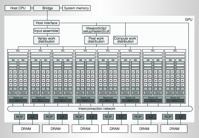
Figure 2: nVIDIA Tesla Architecture (from[10])

As in [14] and [9], we will focus on nVIDIA’s unified graphics and computing platform for GPUs known as the Tesla architecture framework [10] and associated CUDA programming model [1]. However, the discussion and methods presented in this paper apply in general to GPUs that support the OpenCL standard [2] which is very similar to CUDA. A schematic diagram of the Tesla unified GPU architecture is shown in Figure 2. A Tesla GPU consists of an array of streaming processors called Streaming Multiprocessors (SMs). Each SM contains eight processor cores and a small size (16 KB) low latency local shared memory that is shared by its eight processor cores. All SMs are connected to a global DRAM memory through an interconnection network. For example, an nVIDIA GeForce GTX 260 has 27 SMs with a total of 216 processor cores while GTX 285 and Tesla GPUs have 30 SMs with a total of 240 processor cores. A GTX 260 has approximately 900 MB global DRAM memory while GTX 285 and Tesla GPUs have up to 2 GB and 4 GB global DRAM memory, respectively (see Table 1). A GPU’s global DRAM memory is arranged in independent memory partitions. The interconnection network routes the read/write memory requests from the processor cores to the respective global memory partitions, and the results back to the cores. Each global memory partition has its own queue for memory requests and arbitrates among the incoming read/write requests, seeking to maximize DRAM transfer efficiency by grouping read/write accesses to neighboring memory locations. Memory latency to global DRAM memory is optimized when parallel read/write operations can be grouped into a minimum number of arrays of contiguous memory locations.

It is important to note that data accesses from processor cores to their SM’s local shared memory are at least an order of magnitude faster than accesses to global memory. This is an important consideration for any efficient sorting method. Another critical issue for the performance of CUDA implementations is conditional branching. CUDA programs typically execute very large numbers of threads. In fact, a large number of threads is critical for hiding latencies for global memory accesses. The GPU has a hardware thread scheduler that is built to manage tens of thousands and even millions of concurrent threads. All threads are divided into blocks of up to 512 threads, and each block is executed by an SM. An SM executes a thread block by breaking it into groups of 32 threads called warps and executing them in parallel using its eight cores. These eight cores share various hardware components, including the instruction decoder. Therefore, the threads of a warp are executed in SIMT (single instruction, multiple threads) mode, which is a slightly more flexible version of the standard SIMD (single instruction, multiple data) mode. The main problem arises when the threads encounter a conditional branch such as an IF-THEN-ELSE statement. Depending on their data, some threads may want to execute the code associated with the ”true” condition and some threads may want to execute the code associated with the ”false” condition. Since the shared instruction decoder can only handle one branch at a time, different threads can not execute different branches concurrently. They have to be executed in sequence, leading to performance degradation. GPUs provide a small improvement through an instruction cache at each SM that is shared by its eight cores. This allows for a ”small” deviation between the instructions carried out by the different cores. For example, if an IF-THEN-ELSE statement is short enough so that both conditional branches fit into the instruction cache then both branches can be executed fully in parallel. However, a poorly designed algorithm with too many and/or large conditional branches can result in serial execution and very low performance.

3 Previous Work On GPU Sorting

Sorting algorithms for GPUs started to appear a few years ago and have been highly competitive. Early results include GPUTeraSort [6] based on bitonic merge, and adaptive bitonic sort [8] based on a method by Bilardi et.al. [3]. Hybrid sort [16] used a combination of bucket sort and merge sort, and D. Cederman et.al. [4] proposed a quick sort based method for GPUs. Both methods ([16, 4]) suffer from load balancing problems. Until very recently, the comparison-based Thrust Merge method [14] by Nadathur Satish, Mark Harris and Michael Garland of nVIDIA Corporation was considered the best sorting method for GPUs. Thrust Merge uses a combination of odd-even merge and two-way merge, and overcomes the load balancing problems mentioned above. Satish et.al. [14] also presented an even faster GPU radix sort method for the special case of integer sorting. Yet, an upcoming paper by Nikolaj Leischner, Vitaly Osipov and Peter Sanders [9] (to appear in Proc. IPDPS 2010) presents a randomized sample sort method for GPUs that significantly outperforms Thrust Merge [14]. However, as discussed in Section 1, the performance of randomized sample sort can vary with the distribution of the input data because buckets are created through randomly selected data items. Indeed, the performance analysis presented in [9] measures the runtime of their randomized sample sort method for six different data distributions to document the performance variations observed for different input distributions.

4 GPU Bucket Sort:
Deterministic Sample Sort For GPUs

In this section we present GPU Bucket Sort, a deterministic sample sort algorithm for GPUs, and discuss its CUDA implementation. An outline of GPU Bucket Sort is shown in Algorithm 1 below. It consists of a local sort (Step 1), a selection of samples that define balanced buckets (Steps 3-5), moving all data into those buckets (Steps 6-8), and a final sort of each bucket.

Algorithm 1

GPU Bucket Sort (Deterministic Sample Sort For GPUs)

Input: An array $A$ with $n$ data items stored in global memory.

Output: Array $A$ sorted.

1. Split the array $A$ into $m$ sublists $A_{1},...,A_{m}$ containing $\frac{n}{m}$ items each where $\frac{n}{m}$ is the shared memory size at each SM.

2. Local Sort: Sort each sublist $A_{i}$ ($i$=1,…, $m$) locally on one SM, using the SM’s shared memory as a cache.

3. Local Sampling: Select $s$ equidistant samples from each sorted sublist $A_{i}$ ($i$=1,…, $m$) for a total of $sm$ samples.

4. Sorting All Samples: Sort all $sm$ samples in global memory, using all available SMs in parallel.

5. Global Sampling: Select $s$ equidistant samples from the sorted list of $sm$ samples. We will refer to these $s$ samples as global samples.

6. Sample Indexing: For each sorted sublist $A_{i}$ ($i$=1,…, $m$) determine the location of each of the $s$ global samples in $A_{i}$. This operation is done for each $A_{i}$ locally on one SM, using the SM’s shared memory, and will create for each $A_{i}$ a partitioning into $s$ buckets $A_{i1}$,…, $A_{is}$ of size $a_{i1}$,…, $a_{is}$.

7. Prefix Sum: Through a parallel prefix sum operation on $a_{11}$,…, $a_{m1}$, $a_{12}$,…, $a_{m2}$, …, $a_{1s}$,…, $a_{ms}$ calculate for each bucket $A_{ij}$($1\leq i\leq m$, $1\leq j\leq s$, ) its starting location $l_{ij}$ in the final sorted sequence.

8. Data Relocation: Move all $sm$ buckets $A_{ij}$($1\leq i\leq m$, 1$\leq j\leq s$) to location $l_{ij}$. The newly created array consists of $s$ sublists $B_{1}$, …, $B_{s}$ where $B_{j}=A_{1j}\cup A_{2j}\cup...\cup A_{mj}$ for 1$\leq j\leq s$.

9. Sublist Sort: Sort all sublists $B_{j}$, 1$\leq j\leq s$, using all SMs.

— End of Algorithm —

Our discussion of Algorithm 1 and its implementation will focus on GPU performance issues related to shared memory usage, coalesced global memory accesses, and avoidance of conditional branching. Consider an input array $A$ with $n=32M$ data items and a local shared memory size of $\frac{n}{m}=2K$ data items. In Steps 1 and 2 of Algorithm 1, we split the array A into $m=16K$ sublists of $2K$ data items each and then locally sort each of those $m=16K$ sublists. More precisely, we create 16 K thread blocks of 512 threads each, where each thread block sorts one sublist using one SM. Each thread block first loads a sublist into the SM’s local shared memory using a coalesced parallel read from global memory. Note that, each of the 512 threads is responsible for $\frac{n}{m}/512=4$ data items. The thread block then sorts a sublist of $\frac{n}{m}=2K$ data items in the SM’s local shared memory. We tested different implementations for the local shared memory sort within an SM, including quicksort, bitonic sort, and adaptive bitonic sort [3]. In our experiments, bitonic sort was consistently the fastest method, despite the fact that it requires $O(n\log^{2}n)$ work. The reason is that, for Step 2 of Algorithm 1, we always sort $2K$ data items only, irrespective of $n$. For such a small number of items the simplicity of bitonic sort, it’s small constants in the running time, and it’s perfect match for SIMD style parallelism outweigh the disadvantage of additional work. In Step 3 of Algorithm 1, we select $s=64$ equidistant samples from each sorted sublist. The choice of value for $s$ is discussed in Section 5. The implementation of Step 3 is built directly into the final phase of Step 2 when the sorted sublists are written back into global memory. In Step 4, we are sorting all $sm=1M$ selected samples in global memory, using all available SMs in parallel. Here, we compared GPU bitonic sort [6], adaptive bitonic sort [8] based on [3], and randomized sample sort [9]. Our experiments indicate that for up to 16 M data items, simple bitonic sort is still faster than even randomized sample sort [9] due to its simplicity, small constants, and complete avoidance of conditional branching. Hence, Step 4 was implemented via bitonic sort. In Step 5, we select $s=64$ equidistant global samples from the sorted list of $sm=1M$ samples. Here, each thread block/SM loads the $s=64$ global samples into its local shared memory where they will remain for the next step. In Step 6, we determine for each sorted sublist $A_{i}$ ($i$=1, …, $m$) of $\frac{n}{m}=2K$ data items the location of each of the $s=64$ global samples in $A_{i}$. For each $A_{i}$, this operation is done locally by one thread block on one SM, using the SM’s shared memory, and will create for each $A_{i}$ a partitioning into $s=64$ buckets $A_{i1}$,…, $A_{is}$ of size $a_{i1}$,…, $a_{is}$. Here, we apply parallel binary search in $A_{i}$ for each of the global samples. More precisely, we first take the $\frac{s}{2}$-th global sample element and use one thread to perform a binary search in $A_{i}$, resulting in a location $l_{s/2}$ in $A_{i}$. Then we use two threads to perform two binary searches in parallel, one for the $\frac{s}{4}$-th global sample element in the part of $A_{i}$ to the left of location $l_{s/2}$ , and one for the $\frac{3s}{4}$-th global sample element in the part of $A_{i}$ to the right of location $l_{s/2}$. This process is iterated $\log s=6$ times until all $s=64$ global samples are located in $A_{i}$. With this, each $A_{i}$ is split into $s=64$ buckets $A_{i1}$,…, $A_{is}$ of size $a_{i1}$,…, $a_{is}$. Note that, we do not simply perform all $s$ binary searches fully in parallel in order to avoid memory contention within the local shared memory[1]. Step 7 uses a prefix sum calculation to obtain for all buckets their starting location in the final sorted sequence. The operation is illustrated in Figure 1 and can be implemented with coalesced memory accesses in global memory. Each row in Figure 1 shows the $a_{i1}$,…, $a_{is}$ calculated for each sublist. The prefix sum is implemented via a parallel column sum (using all SMs), followed by a prefix sum on the columns sums (on one SM in local shared memory), and a final update of the partial sums in each column (using all SMs). In Step 8, the $sm=1M$ buckets are moved to their correct location in the final sorted sequence. This operation is perfectly suited for a GPU and requires one parallel coalesced data read followed by one parallel coalesced data write operation. The newly created array consists of $s=64$ sublists $B_{1}$, …, $B_{s}$ where each $B_{j}=A_{1j}\cup A_{2j}\cup...\cup A_{mj}$ has at most $\frac{2n}{s}=1M$ data items [15]. In Step 9, we sort each $B_{j}$ using the same bitonic sort implementation as in Step 4. Note that, since each $B_{j}$ is smaller than $16M$ data items, simple bitonic sort is faster for each $B_{j}$ than even randomized sample sort [9] due to bitonic sort’s simplicity, small constants, and complete avoidance of conditional branching.

Figure 1: Illustration Of Step 7 In Algorithm 1

5 Experimental Results And Discussion

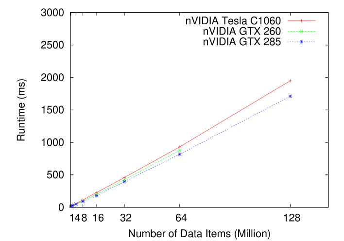
Figure 4: Performance Of Deterministic Sample Sort For GPUs (GPU Bucket Sort). Total runtime for varying number of data items on different GPUs: nVIDIA Tesla C1060, GTX 260 and GTX 285.

For our experimental evaluation, we executed Algorithm 1 on three different GPUs (nVIDIA Tesla, GTX 285, and GTX 260) for various data sets of different sizes, and compared our results with those reported in [14] and [9] which are the current best GPU sorting methods. Table 1 shows some important performance characteristics of the three different GPUs. The Tesla and GTX 285 have more cores than the GTX 260. The GTX 285 has the highest core clock rate and in summary the highest level of core computational power. The Tesla has the largest memory but the GTX 285 has the best memory clock rate and memory bandwidth. In fact, even the GTX 260 has a higher clock rate and memory bandwidth than the Tesla C1060. Figure 4 shows a comparison of the runtime of our GPU Bucket Sort method on the Tesla C1060, GTX 260 and GTX 285 (with 2 GB memory) for varying number of data items. Each data point shows the average of 100 experiments. The observed variance was less than 1 ms for all data points since GPU Bucket Sort is deterministic and any fluctuation observed was due to noise on the GPU (e.g. operating system related traffic). All three curves show a growth rate very close to linear which is encouraging for a problem that requires $O(n\log n)$ work. GPU Bucket Sort performs better on the GTX 285 than both Tesla and GTX 260. Furthermore, it performs better on the GTX 260 than on the Tesla C1060. This indicates that GPU Bucket Sort is memory bandwidth bound which is expected for sorting methods since the sorting problem requires only very little computation but a large amount of data movement. For individual steps of GPU Bucket Sort, the order can sometimes be reversed. For example, we observed that Step 2 of Algorithm 1 (local sort) runs faster on the Tesla C1060 than on the GTX 260 since this step is executed locally on each SM and its performance is largely determined by the number of SMs and the performance of the SM’s cores. However, the GTX 285 remained the fastest machine, even for all individual steps.

We note that GPU Bucket Sort can sort up to $n=64M$ data items within the 896 MB memory available on the GTX 260 (see Figure 4). On the GTX 285 with 2 GB memory and Tesla C1060 our GPU Bucket Sort method can sort up to $n=256M$ and $n=512M$ data items, respectively (see Figures 6&7).

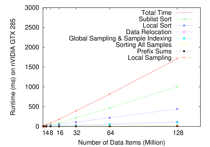
Figure 5: Performance Of Deterministic Sample Sort For GPUs (GPU Bucket Sort). Total runtime and runtime for individual steps of Algorithm 1 on an nVIDIA GTX 285 for varying number of data items.

Figure 5 shows in detail the time required for the individual steps of Algorithm 1 when executed on a GTX 285. We observe that sublist sort (Step 9) and local sort (Step 2) represent the largest portion of the total runtime of GPU Bucket Sort. This is very encouraging in that the “overhead” involved to manage the deterministic sampling and generate buckets of guaranteed size (Steps 3-7) is small. We also observe that the data relocation operation (Step 8) is very efficient and a good example of the GPU’s great performance for data parallel access when memory accesses can be coalesced (see Section 2). Note that, for Algorithm 1 the sample size $s$ is a free parameter. With increasing $s$, the sizes of sublists $B_{j}$ created in Step 8 of Algorithm 1 decrease and the time for Step 9 decreases as well. However, the time for Steps 3-7 grows with increasing $s$. This trade-off is illustrated in Figure 3 which shows the total runtime for Algorithm 1 as a function of $s$ for fixed $n=32M,64M,128M$. As shown in Figure 3, the total runtime is smallest for $s=64$, which is the parameter chosen for our GPU Bucket Sort code.

Figures 6 and 7 show a comparison between GPU Bucket Sort and the current best GPU sorting methods, Randomized Sample Sort [9] and Thrust Merge Sort [14]. Figure 6 shows the runtimes for all three methods on a GTX 285 and Figure 7 shows the runtimes of all three methods on a Tesla C1060. Note that, [14] and [9] did not report runtimes for the GTX 260. For GPU Bucket Sort, all runtimes are the averages of 100 experiments, with less than 1 ms observed variance. For Randomized Sample Sort and Thrust Merge Sort, the runtimes shown are the ones reported in [9] and [14]. For Thrust Merge Sort, performance data is only available for up to $n=16M$ data items. For larger values of $n$, the current Thrust Merge Sort code shows memory errors [5]. As reported in [9], the current Randomized Sample Sort code can sort up to $32M$ data items on a GTX 285 with 1 GB memory and up to $128M$ data items on a Tesla C1060. Our GPU Bucket Sort code appears to be more memory efficient. GPU Bucket Sort can sort up to $n=256M$ data items on a GTX 285 with 2GB memory and up to $n=512M$ data items on a Tesla C1060. Therefore, Figures 6a and 7a show the performance comparison with higher resolution for up to $n=64M$ and $n=128M$, respectively, while Figures 6b and 7b show the performance comparison for the entire range up to $n=256M$ and $n=512M$, respectively.

We observe in Figures 6a and 7a that, as reported in [9], Randomized Sample Sort [9] significantly outperforms Thrust Merge Sort [14]. Most importantly, we observe that Randomized Sample Sort [9] and our Deterministic Sample Sort (GPU Bucket Sort) show nearly identical performance on both, the GTX 285 and Tesla C1060. Note that, the experiments in [9] used a GTX 285 with 1 GB memory whereas we used a GTX 285 with 2 GB memory. As shown in Table 1, the GTX 285 with 1 GB has a slightly better memory clock rate and memory bandwidth than the GTX 285 with 2 GB which implies that the performance of Deterministic Sample Sort (GPU Bucket Sort) on a GTX 285 is actually a few percent better than the performance of Randomized Sample Sort. The data sets used for the performance comparison in Figures 6 and 7 were uniformly distributed, random data items. The data distribution does not impact the performance of Deterministic Sample Sort (GPU Bucket Sort) but has an impact on the performance of Randomized Sample Sort. In fact, the uniform data distribution used for Figures 6 and 7 is a best case scenario for Randomized Sample Sort where all bucket sizes are nearly identical.

Figures 6b and 7b show the performance of GPU Bucket Sort for up to $n=256M$ and $n=512M$, respectively. For both architectures, GTX 285 and Tesla C1060, we observe a very close to linear growth rate in the runtime of GPU Bucket Sort for the entire range of data sizes. This is very encouraging for a problem that requires $O(n\log n)$ work. In comparison with Randomized Sample Sort, the linear curves in Figures 6b and 7b show that our GPU Bucket Sort method maintains a fixed sorting rate (number of sorted data items per time unit) for the entire range of data sizes, whereas it is shown in [9] that the sorting rate for Randomized Sample Sort fluctuates and often starts to decrease for larger values of $n$.

6 Conclusions

In this paper, we presented a deterministic sample sort algorithm for GPUs, called GPU Bucket Sort. Our experimental evaluation indicates that GPU Bucket Sort is considerably faster than Thrust Merge [14], the best comparison-based sorting algorithm for GPUs, and it is exactly as fast as the new Randomized Sample Sort for GPUs [9] when the input data sets used are uniformly distributed, which is a best case scenario for Randomized Sample Sort. However, as observed in [9], the performance of Randomized Sample Sort fluctuates with the input data distribution whereas GPU Bucket Sort does not show such fluctuations. In fact, GPU Bucket Sort showed a fixed sorting rate (number of sorted data items per time unit) for the entire range of data sizes tested (up to $n=512M$ data items). In addition, our GPU Bucket Sort implementation appears to be more memory efficient because GPU Bucket Sort is able to sort considerably larger data sets within the same memory limits of the GPUs.

	Tesla C1060	GTX 285 (2 GB)	GTX 285 (1 GB)	GTX 260
Number Of Cores	240	240	240	216
Core Clock Rate	602 MHz	648 MHz	648 MHz	576 MHz
Global Memory Size	4 GB	2 GB	1 GB	896 MB
Memory Clock Rate	1600 MHz	2322 MHz	2484 MHz	1998 MHz
Memory Bandwidth	102 GB/sec	149 GB/sec	159 GB/sec	112 GB/sec

Table 1: Performance Characteristics For nVIDIA Tesla C1060, GTX 285 with 2 GB memory, GTX 285 with 1 GB memory, and GTX 260. (Source: [13, 12, 11])

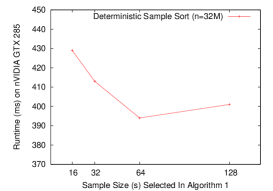
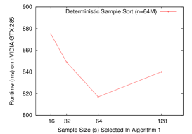
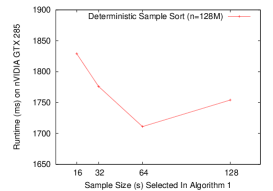
Figure 3: Runtime Of Algorithm 1 As A Function Of Selected Sample Size $s$ For Fixed $n=32M$, $n=64M$, and $n=128M$.

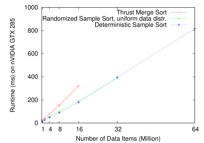
(a) Number of Data Items Up To 64,000,000.

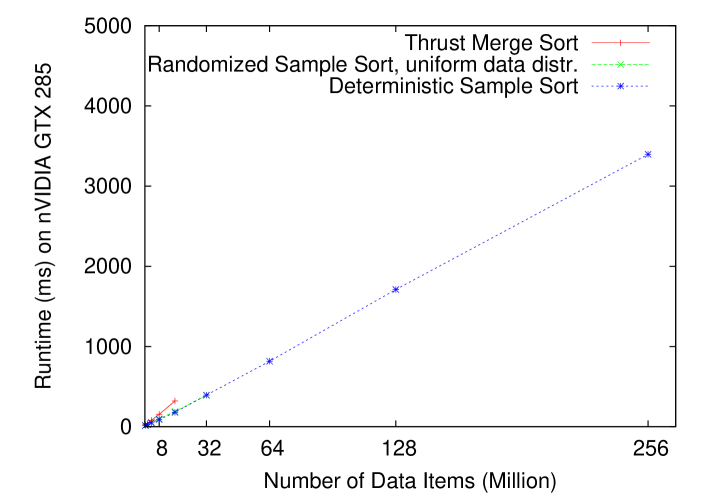
(b) Number of Data Items Up To 512,000,000.

Figure 6: Comparison between Deterministic Sample Sort (GPU Bucket Sort), Randomized Sample Sort [9] and Thrust Merge Sort [14]. Total runtime for varying number of data items on an nVIDIA GTX 285. ([14] and [9] provided data only for up to 16M and 32M data items, respectively.)

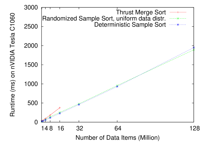
(a) Number of Data Items Up To 128,000,000.

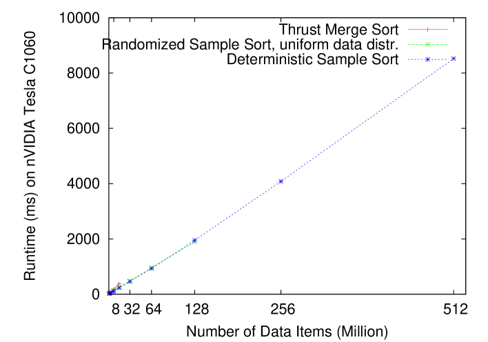
(b) Number of Data Items Up To 512,000,000.

Figure 7: Comparison between Deterministic Sample Sort (GPU Bucket Sort), Randomized Sample Sort [9] and Thrust Merge Sort [14]. Total runtime for varying number of data items on an nVIDIA Tesla C1060.([14] and [9] provided data only for up to 16M and 128M data items, respectively.)

References

- [1] NVIDIA CUDA Programming Guide. nVIDIA Corporation, 2009.
- [2] The OpenCL Specification 1.0. Khronos OpenCL Working Group, 2009.
- [3] G. Bilardi and A. Nicolau. Adaptive bitonic sorting. An optimal parallel algorithm for shared-memory machines. SIAM J Comput, 18(2):216–228, 1989.
- [4] D. Cederman and P. Tsigas. A practical quicksort algorithm for graphics processors. In Proc. European Symposium on Algorithms (ESA), volume 5193 of LNCS, pages 246–258, 2008.
- [5] M. Garland. Private communication. nVIDIA Corporation, 2009.
- [6] N. Govindaraju, J. Gray, R. Kumar, and D. Manocha. GPUTeraSort: high performance graphics co-processor sorting for large database management. In Proc. International Conference on Management of Data (SIGMOD), pages 325 – 336, 2006.
- [7] GPGPU.ORG. General-purpose computation on graphics hardware. http://gpgpu.org/tag/papers.
- [8] A. Greb and G. Zachmann. GPU-ABiSort: Optimal parallel sorting on stream architectures. In Proc. Int’l Parallel and Distributed Processing Symposium (IPDPS), 2006.
- [9] N. Leischner, V. Osipov, and P. Sanders. GPU sample sort. In Proc. Int’l Parallel and Distributed Processing Symposium (IPDPS), to appear, 2010 (currently available at http://arxiv1.library.cornell.edu/abs/0909.5649).
- [10] E. Lindholm, J. Nickolls, S. Oberman, and J. Montrym. Nvidia tesla: A unified graphics and computing architecture. IEEE Micro, 28(2):39–55, 2008.
- [11] nVIDIA Corporation. Gtx 260 GPU specification. http://www.nvidia.com/object/product_geforce_gtx_260_us.html.
- [12] nVIDIA Corporation. Gtx 285 GPU specification. http://www.nvidia.com/object/product_geforce_gtx_285m_us.html.
- [13] nVIDIA Corporation. Tesla c1060 GPU specification. http://www.nvidia.com/object/product_tesla_c1060_us.html.
- [14] N. Satish, M. Harris, and M. Garland. Designing efficient sorting algorithms for manycore GPUs. In Proc. Int’l Parallel and Distributed Processing Symposium (IPDPS), 2009.
- [15] H. Shi and J. Schaeffer. Parallel sorting by regular sampling. J. Par. and Dist. Comp., 14:362–372, 1992.
- [16] E. Sintorn and U. Assarsson. Fast parallel GPU-sorting using a hybrid algorithm. J. of Parallel and Distributed Computing, 68(10):1381–1388, 2008.