Quantum Quenches in a $XXZ\,$ Spin Chain from a Spatially Inhomogeneous Initial State

Abstract

Results are presented for the nonequilibrium dynamics of a quantum $XXZ$-spin chain whose spins are initially arranged in a domain wall profile via the application of a magnetic field in the $z$-direction which is spatially varying along the chain. The system is driven out of equilibrium in two ways: a). by rapidly turning off the magnetic field, b). by rapidly quenching the interactions at the same time as the magnetic field is turned off. The time-evolution of the domain wall profile as well as various two-point spin correlation functions are studied by the exact solution of the fermionic problem for the $XX$ chain and via a bosonization approach and a mean-field approach for the $XXZ$ chain. At long times the magnetization is found to equilibrate (reach the ground state value), while the two-point correlation functions in general do not. In particular, for quenches within the gapless $XX$ phase, the spin correlation function transverse to the $z$ direction acquires a spatially inhomogeneous structure at long times whose details depend on the initial domain wall profile. The spatial inhomogeneity is also recovered for the case of classical spins initially arranged in a domain wall profile and shows that the inhomogeneities arise due to the dephasing of transverse spin components as the domain wall broadens. A generalized Gibbs ensemble approach is found to be inadequate in capturing this spatially inhomogeneous state.

I Introduction

Recent years have seen remarkable progress in manipulating cold-atom systems rev08 providing us with almost ideal realizations of strongly correlated many-particle systems. Cold atom systems also have the unique feature that the interactions between particles and the external potentials that they are subjected to are highly tunable and can be changed rapidly in time, thus driving these systems into highly nonequilibrium states Weiss06 . This property has in turn motivated a lot of theoretical activity that revolves around studying nonequilibrium time-evolution of strongly correlated systems arising due to a sudden change in some parameter of the Hamiltonian referred to as a “quantum quench”. The general consensus is that if the strongly correlated system is integrable, its time-evolution from some arbitrary initial state is highly constrained by the initial conditions so that these systems do not reach the ground state but instead reach interesting nonequilibrium time-dependent or time-independent steady states.

In this paper we study quenched dynamics in one such integrable model, namely the $XXZ$ spin chain. This model shows rich behavior even in its ground state giamarchi . For example, it exhibits a quantum critical point at $J_{z}=\pm J$ where $J$ is the exchange interactions for the $x,y$ components of the spins, and $J_{z}$ is the exchange interaction for the $z$ component of the spins. For $|J/J_{z}|>1$, the ground state is an $XX$ phase characterized by gapless excitations, while for $|J/J_{z}|<1$, the spins are in an Ising phase where the excitation spectrum has a gap. Note that the special point in the gapless phase corresponding to $J_{z}=0$ will be referred to as the XX-model, while the term gapless $XX$ phase will refer to the regime $|J/J_{z}|>1$.

Nonequilibrium dynamics of the $XXZ$ model arising due to quenches has been a very active area of research (see for example Sengupta04 ; Demler09 ). While most previous work has studied quenched dynamics in spatially homogeneous systems, in this work we consider the nonequilibrium time-evolution arising from quenching from an initial state which is spatially inhomogeneous. Such an initial state is created by the application of an external magnetic field in the $z$ direction that varies in magnitude along the chain, changing its sign at some point so that the spins are aligned in a domain wall pattern. (See Weld09 for an experimental realization of such a setup). We study nonequilibrium dynamics that arise in the following two ways: a). by a sudden quench of the magnetic field to zero; b). by a sudden quench of the magnetic field to zero along with a quench in the magnitude of the exchange interactions. Note that the above are situations where the time evolution is due to a final Hamiltonian that has a spatially homogeneous ground state. We would like to understand how the system evolves in time after the quench, and whether the initial inhomogeneity affects the properties of the system at long times.

Some literature already exists which studies time evolution of a spin chain initially arranged in a domain wall profile. Antal et al antal study the time evolution of a sharp domain wall in the exactly solvable $XX$ model and find ballistic broadening of the domain wall width. Similar studies for the time-evolution of a domain wall has been carried out for the XX model Karevski01 ; Ogata02 ; Platini07 and the critical transverse spin Ising model Karevski01 ; Platini05 . The numerical method time-dependent density matrix renormalization group (t-DMRG) has been used to study the time-evolution of a domain wall both in the gapless phase as well as the gapped Ising phase of an $XXZ$ chain tdmrg05 ; tdmrg09 . Their study reveals qualitatively different behavior in the two phases, with ballistic broadening of the domain wall in the gapless phase, and more complicated non-ballistic behavior in the Ising phase. In addition conformal field theory methods Calabrese08 have been used to study both the time-evolution of the domain wall profile as well as two-point correlation functions for the Ising chain. Studies also exist on the time-evolution of other quantities such as the entanglement entropy after a quench from a spatially inhomogeneous initial state Eisler09 ; localquench . Thus what is lacking in the literature is the study of the time evolution of two-point correlation functions for the $XXZ$ chain from an initial inhomogeneous state. The advantage of studying these quantities is that they are often more sensitive to nonequilibrium initial conditions than averages of local quantities such as the magnetization.

In this paper we extend previous results by studying the time evolution of both the local magnetization as well as two point correlation functions related to the longitudinal (along $z$ direction) and the transverse spin correlation function for the $XXZ$ chain. In addition we use a variety of theoretical methods such as bosonization, exact solution of the fermionic problem as well as a classical treatment of spins which allows us to compare the relative merits of these approximations. Consistent with previous results, we find that the magnetization always equilibrates (i.e, reaches the ground state value). In addition the details of how the domain wall profile evolves in time depend on whether the system after the quench is in the gapless phase or the gapped Ising phase tdmrg05 ; tdmrg09 . For example in the gapless phase the domain wall is found to spread out ballistically, however in the gapped phase the dynamics is much more complicated showing oscillations and revivals at short time scales.

In studying the time-evolution of two-point correlation functions we obtain the interesting new result that the transverse spin-correlation function shows a lack of equilibration reaching a nonequilibrium steady state that is also spatially inhomogeneous. The length scale of the spatial inhomogeneity is found to depend on the details of the initial domain wall profile and is found to arise due to the dephasing of transverse spin components as the domain wall broadens. This result is qualitatively different from those obtained for the Ising chain initially arranged in a domain wall profile where no residual inhomogeneity was observed Calabrese08 .

The paper is organized as follows. In section II we study the XX model which is initially subjected to a spatially varying magnetic field so that the spins are arranged in a domain wall profile. We study the nonequilibrium dynamics that arises when this magnetic-field is suddenly switched off. These results are obtained for two cases. One for an initial external magnetic field that varies linearly in position and is equivalent to an effective electric field on the fermions. The second case is that of an initial magnetic field which has a sharp step-function profile. In section III the effect of quenching only a spatially varying magnetic field in the XX model is studied via a bosonization approach. The results of section II and III are found to be in qualitative agreement and in particular recover ballistic domain wall motion and spatial inhomogeneities in the transverse spin correlation function. A physical explanation for this inhomogeneity is provided in section IV where the problem of quenching a spatially varying magnetic field is studied classically and a spin-wave pattern is obtained as a long time solution of a Landau-Lifshitz equation.

In section V, the effect of simultaneously quenching the magnetic field and interactions is studied using a bosonization approach. In section V.1 results are presented for the case when the quench is entirely within the gapless XX phase. The spatial inhomogeneities in the correlation functions are recovered along with the nonequilibrium exponents obtained earlier in a purely homogeneous interaction quench cazalilla1 ; cazalilla . In section V.2 the effect of quenching into the gapped Ising phase is studied via a semiclassical approach. Here we find the domain wall dynamics to be qualitatively different, however at long times we find that all inhomogeneities eventually decay away. The latter result may very well be an artifact of the semiclassical approach which neglects creation of solitons. The results of the semiclassical approach is complemented by a mean-field treatment in section VI where we address the question of whether Ising order can develop for a system initially in a domain wall state. Finally we conclude in section VII.

II Quench of a spatially varying magnetic field in the XX model: Exact solution of the fermionic problem

In this section we will study the XX model with a magnetic field in the $z$ direction that varies linearly in position and changes sign at the center of the spin chain, so that the ground state is a domain wall configuration. In subsection II.1 we will study the properties of this domain wall state, and in subsequent subsections study the nonequilibrium time-evolution arising when the the spatially varying magnetic field is suddenly switched off.

II.1 Creation of domain-wall state

Our starting point is the $XX$ Hamiltonian in a magnetic field,

$$H_{xx}=-J\sum_{j}\left[S_{j}^{x}S_{j+1}^{x}+S_{j}^{y}S_{j+1}^{y}-\frac{h_{j}}{J}S_{j}^{z}\right],$$ (1)

where $S_{j}^{\nu}=\frac{1}{2}\sigma_{j}^{\nu}$, $\sigma^{\nu}$ are Pauli matrices, $h_{j}$ is an external magnetic field aligned along the $\hat{z}$ direction, and $J$ is the exchange energy. For a uniform magnetic field one commonly employs the Jordan-Wigner transformation lsm ; barouch1 ; barouch2 ; barouch3 to map the spin system to a system of spin-less non-interacting fermions which can be easily diagonalized (for details see Appendix A).

To create an inhomogeneous state we will consider a linearly varying field $h_{j}={\cal F}ja$, where $a$ is a lattice spacing. Note that the ground state properties of spin-chains in various spatially varying magnetic fields has been studied in DWstatics . After the Jordan-Wigner transformation Eq. 1 for $h_{j}={\cal F}ja$ maps to the Wannier-Stark problem Eisler09 ; smith ; case of electrons in a lattice subjected to a constant force (or electric field) ${\cal F}$,

$$H_{xx}=-\frac{J}{2}\sum_{j}\left[c_{j}^{\dagger}c_{j+1}+c_{j+1}^{\dagger}c_{j}\right]+\sum_{j}j\mathcal{F}ac_{j}^{\dagger}c_{j}$$ (2)

This Hamiltonian can be diagonalized as follows,

$$H_{xx}=\sum_{m}\epsilon_{m}\eta_{m}^{\dagger}\eta_{m},$$ (3)

where

$$\epsilon_{m}=m\mathcal{F}a,\;\;\;\;\;\left(\forall\;\;m\;=\;\mbox{integer}\right),$$ (4)

and

$$\eta_{m}^{\dagger} = \sum_{j}J_{j-m}\left(\frac{J}{\mathcal{F}a}\right)c^{\dagger}_{j}$$ (5)

$$= \frac{1}{\sqrt{N}}\sum_{k}\exp\left[-ikma-i\frac{J}{\mathcal{F}a}\sin(ka)\right]c^{\dagger}_{k}$$ (6)

Above $c_{j}=\frac{1}{\sqrt{N}}\sum_{k}c_{k}e^{ikj}$, $N$ is the total number of sites and $J_{n}(x)\,$ is a Bessel function of the first kind.

We construct the ground state $\left|\Psi\right\rangle$ by including all negative energy states,

$$\left|\Psi\right\rangle=\prod_{m<0}\eta_{m}^{\dagger}\left|0\right\rangle.$$ (7)

This is a domain-wall state with a characteristic width $\frac{x}{a}\equiv\alpha=\frac{J}{\mathcal{F}a}$ to the left (right) of which all spins are up (down). This can be seen by evaluating the magnetization at the position $ja$

$$m^{z}(j)=\left\langle\Psi|c_{j}^{\dagger}c_{j}|\Psi\right\rangle-\frac{1}{2}.$$ (8)

which on rewriting $c_{j},c_{j}^{\dagger}$ in terms of the $\eta_{m}$ operators and evaluating the expectation value is found to be

$$m^{z}(j)=-\frac{1}{2}+\sum_{m\geq 0}J^{2}_{j+m}(\alpha)$$ (9)

Upon noting that the support of $J_{n}(x)\,$ is restricted to hartmann $|n|\leq x$, and using the identity abramowitz $\sum_{n}J_{n}^{2}(x)=1$, it is easy to see that this indeed describes a domain-wall state of width $\alpha$. Eq. 9 is also plotted in Fig. 1.

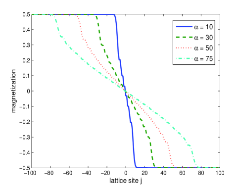
Figure 1: (Color online) Plot of the initial magnetization for various values of the domain wall width $\alpha=\frac{J}{\mathcal{F}a}$.

It is worth noting that the case of $\alpha=0$ corresponds to an infinite “electric field” $\mathcal{F}$ that forces a sharp wall of zero width. This case was investigated by Antal et alantal . We will extend some of their results to more general domain walls, and also study spin-spin correlation functions.

The basic spin correlation functions that we will compute are,

$$C^{\nu\nu}(j,j+n)=\left\langle S_{j}^{\nu}S_{j+n}^{\nu}\right\rangle,\;\;\;\;(\nu=x,z)$$ (10)

where we will refer to $C^{zz}$ ($C^{xx}$) as the longitudinal (transverse) spin correlation function. These may be expressed in terms of Majorana operators lsm $A_{j}=c_{j}^{\dagger}+c_{j}$, and $B_{j}=c_{j}^{\dagger}-c_{j}$ as follows,

$$C^{zz}(j,j+n)=\frac{1}{4}\left\langle B_{j}A_{j}B_{j+n}A_{j+n}\right\rangle,$$ (11)

and

$$C^{xx}(j,j+n)=\frac{1}{4}\left\langle B_{j}A_{j+1}B_{j+1}\cdots A_{j+n-1}B_{j+n-1}A_{j+n}\right\rangle,$$ (12)

The above correlations can be evaluated by rewriting $c_{i}$ in terms of $\eta_{m}$ and applying Wick’s theorem. The basic contractions are zeromode

$$\left\langle B_{j}A_{j+n}\right\rangle=-\left\langle A_{j}B_{j+n}\right\rangle=\sum_{m>0}\left[J_{j+m}(\alpha)J_{j+n+m}(\alpha)\right.$$

$$\left.-J_{j-m}(\alpha)J_{j+n-m}(\alpha)\right],$$ (13)

$$\left\langle A_{j}A_{j+n}\right\rangle=-\left\langle B_{j}B_{j+n}\right\rangle=\delta_{n=0}.$$ (14)

Using some Bessel function identities, the mixed contraction can be simplified to

$$\left\langle B_{j}A_{j+n}\right\rangle=\frac{\alpha}{2n}\left[J_{j+n}(\alpha)J_{j+1}(\alpha)-J_{j+n+1}(\alpha)J_{j}(\alpha)\right.$$

$$\left.-J_{j+n}(\alpha)J_{j-1}(\alpha)+J_{j+n-1}(\alpha)J_{j}(\alpha)\right].$$ (15)

Since we encounter no contractions of the form $\left\langle A_{i}A_{i}\right\rangle$, the function $C^{xx}(j,j+n)\,$ may be writtenlsm as a Toeplitz determinant which is a computationally cheap task. In the next sub-section when we evaluate the correlation functions after a quench of the magnetic field, we will find $\left\langle A_{j}A_{j+n}\right\rangle\neq 0$ in the nonequilibrium state. In this case, the evaluation of $C^{xx}$ will require computing the square root of a determinant barouch2 .

The correlation functions $C^{zz}$ and $C^{xx}$ for $\alpha=50$ are given in Fig. 2 and Fig. 3 respectively. The main point to notice here is that close to the center of the domain wall where the external magnetic field is small, the correlations tend to mimic those in the ground state of the homogeneous ($h_{j}=0$) $XX$ model. For example, the nearest neighbor longitudinal spin correlation function in the absence of a magnetic field is barouch3 $C^{zz}_{eq}(n=1)=-\frac{1}{\pi^{2}}$. This is precisely the value that the $C^{zz}(j,j+1)$ correlation function takes in Fig. 2 at the center of the domain wall.

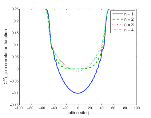
Figure 2: (Color online) Plot of $C^{zz}(j,j+n)\,$ for $n=1,2,3,4$ and $\alpha=\frac{J}{{\cal F}a}=50$.

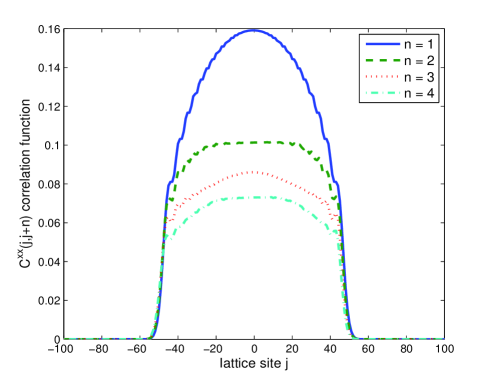
Figure 3: (Color online) Plot of $C^{xx}(j,j+n)\,$ for $n=1,2,3,4$ and $\alpha=\frac{J}{{\cal F}a}=50$.

II.2 Domain wall dynamics after the magnetic field quench

We will now explore the dynamics that arises when the spatially varying magnetic field is suddenly switched off at $t=0$ i.e., $h_{j}(t)=\theta(-t)\mathcal{F}ja$. Thus at $t<0$ the many-body wavefunction of the system is Eq. 7, while for $t>0$, as shown in Appendix A, the wave-function evolves according to the Hamiltonian,

$$H_{f}=\sum_{k}\epsilon_{k}c_{k}^{\dagger}c_{k}$$ (16)

where $\epsilon_{k}=-J\cos(ka)$.

The time-dependent magnetization is given by

$$m^{z}(j,t)=\left\langle\Psi\right|c_{j}^{\dagger}(t)c_{j}(t)\left|\Psi\right\rangle-\frac{1}{2}.$$ (17)

The time-evolution of $c_{j},c_{j}^{\dagger}$ in terms of the $\eta_{m}$ operators is given in Eqns. 152, 153 from which we obtain

$$m^{z}(j,t)=-\frac{1}{2}+\sum_{m>0}|L(j+m,t,\alpha)|^{2},$$ (18)

where Eisler09

$$L(j+m,t,\alpha)=\int_{-\pi}^{\pi}\frac{dk}{2\pi}e^{ik(j+m)-i\epsilon_{k}t-i\alpha\sin k}.$$ (19)

Evaluating the integral, we find

$$m^{z}(j,t)=-\frac{1}{2}+\sum_{m>0}J^{2}_{j+m}\left(\sqrt{(Jt)^{2}+\alpha^{2}}\right).$$ (20)

This corresponds to a wall whose width $W=\sqrt{(Jt)^{2}+\alpha^{2}}$ increases linearly and hence ballistically in time with a velocity of $Ja$ for times $t>\alpha/J$. Setting $\alpha=0$, we recover the result of Antal et al antal . Note that the time-evolution of the entanglement for general $\alpha$ has been studied in Eisler09 .

II.3 Correlation functions after the magnetic field quench

We now turn to the evaluation of the longitudinal and transverse correlation functions given in Eqns. (11) and  (12) at a time $t$ after the quench. The basic contractions that we need are $\left\langle B_{j}(t)A_{j+n}(t)\right\rangle$ and $\left\langle A_{j}(t)A_{j+n}(t)\right\rangle$ for which we find the following expressions

$$\left\langle B_{j}(t)A_{j+n}(t)\right\rangle=$$

$$\frac{r}{2n}\left[e^{in\delta}\left(J_{j+n}(r)J_{j+1}(r)-J_{j+n+1}(r)J_{j}(r)\right)\right.$$

$$\left.-e^{-in\delta}\left(J_{j+n}(r)J_{j-1}(r)-J_{j+n-1}(r)J_{j}(r)\right)\right],$$ (21)

$$\left\langle A_{j}(t)A_{j+n}(t)\right\rangle=$$

$$\frac{r}{2n}\left[e^{in\delta}\left(J_{j+n}(r)J_{j+1}(r)-J_{j+n+1}(r)J_{j}(r)\right)\right.$$

$$\left.+e^{-in\delta}\left(J_{j+n}(r)J_{j-1}(r)-J_{j+n-1}(r)J_{j}(r)\right)\right],$$ (22)

with $r=\sqrt{(Jt)^{2}+\alpha^{2}}\,$ and $\tan\delta\equiv Jt/\alpha$. As before, we have $\left\langle B_{j}(t)B_{j+n}(t)\right\rangle=-\left\langle A_{j}(t)A_{j+n}(t)\right\rangle$ and $\left\langle B_{j}(t)A_{j+n}(t)\right\rangle=-\left\langle A_{j}(t)B_{j+n}(t)\right\rangle$.

The transverse correlation function $C^{xx}(j,j+n,t)$ is given by

$$|C^{xx}(j,j+n,t)|=\frac{1}{4}\sqrt{\mbox{det}{\bf C}},$$ (23)

where ${\bf C}\,$ is the anti-symmetric matrix

$${\bf C}=\left(\begin{array}[]{cc}{\bf S}&{\bf G}\\ {\bf-G}&{\bf Q}\end{array}\right),$$ (24)

with the $n\times n\,$ sub-matrices defined by

$$S_{ik}=-S_{ki} = \left\langle B_{i+j-1}B_{k+j-1}\right\rangle\;\;(k>i)$$ (25)

$$Q_{ik}=-Q_{ki} = \left\langle A_{i+j}A_{k+j}\right\rangle\;\;(k>i)$$ (26)

$$G_{ik} = \left\langle B_{i+j-1}A_{k+j}\right\rangle.$$ (27)

Note that both ${\bf S}\,$ and ${\bf Q}\,$ are anti-symmetric, and thus defined by the elements with $k>i$, while no such restriction is placed on ${\bf G}$.

The numerical evaluation of the above expression for $\alpha=25$ is shown in Fig. 4 for three different times: $t=0$, an intermediate time and for long times where one finds the appearance of a spatially oscillating pattern at the scale of the Fermi-wave vector $k_{F}=\pi/2$.

In order to get some insight into the long time behavior of the system, we consider the limit of $r\rightarrow\infty$ while imposing the condition $j,j+n\ll r$ on the two position indices of the correlation functions. This limit corresponds to a very broad domain wall which may arise either due to a very weak electric field $\alpha\gg 1$ at arbitrary times $t$ (and hence arbitrary $\delta$) or could arise on waiting long enough after a quench so that an initial narrow domain wall has had enough time to broaden. The condition on the position indices imply that we are looking at correlations in the vicinity of the center of the domain wall where the magnetization has locally equilibrated. Using the asymptotic expansion for the Bessel functions with large arguments abramowitz , we find

$$\left\langle B_{j}(t)A_{j+n}(t)\right\rangle\sim\frac{2\cos(n\delta)}{\pi n}\sin\left(\frac{n\pi}{2}\right),$$ (28)

$$\left\langle A_{j}(t)A_{j+n}(t)\right\rangle\sim\frac{2i\sin(n\delta)}{\pi n}\sin\left(\frac{n\pi}{2}\right)$$ (29)

Substituting the asymptotic expansions in Eq. 28, Eq. 29 we find,

$$C^{zz}(j,j+n,t)\longrightarrow C^{zz}_{eq}(n)=-\frac{\sin^{2}\left(\frac{\pi n}{2}\right)}{\pi^{2}n^{2}}$$ (30)

where $C^{ab}_{eq}(n)$ is the equilibrium result (i.e. the result in the ground state of $H_{f}$) for the $ab$ correlation function barouch3 .

Employing the asymptotic expansions in the evaluation of $C^{xx}(j,j+n)$, we have verified through $n\sim 1000\,$ that

$$C^{xx}(j,j+n,t) =C^{xx}_{eq}(n)\cos(n\delta)$$ (32)

$$\xrightarrow{t\rightarrow\infty}C^{xx}_{eq}(n)\cos\left(\frac{\pi n}{2}\right)$$

where $C_{eq}^{xx}(n)\,$ is the equilibrium value of the $xx$-correlation function lsm which has the asymptotic form ovchinnikov ,

$$C^{xx}_{eq}(n)\approx\frac{1}{\sqrt{8n}}\kappa^{2},$$ (33)

with $\log\kappa=\frac{1}{4}\int_{0}^{\infty}\frac{dt}{t}\left(e^{-4t}-\frac{1}{\cosh^{2}t}\right)$.

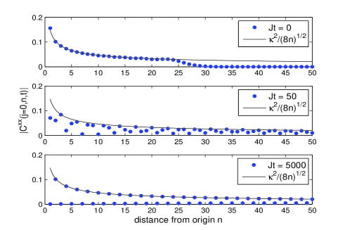
Figure 4: (Color online) Time evolution of $C^{xx}(j=0,n)$ correlation function for $\alpha=25$. Solid line is the equilibrium correlation function $C^{xx}_{eq}$.

The appearance of these oscillations at a wave-length of $\lambda=4$ where

$$C^{xx}(j,j+n,t)\xrightarrow{t\rightarrow\infty}C^{xx}_{eq}(n)\cos(\frac{2\pi n}{\lambda})$$ (34)

is indeed intriguing. To understand better what sets this length scale, we study more general initial domain walls. The one considered so far has the maximum possible positive (negative) polarization of $S_{z}=\pm 1/2$ on the left (right) ends of the domain wall, with a width of the domain wall controlled by $\alpha=\frac{J}{{\cal F}a}$. Antal et al antal have shown how to construct domain walls of zero width ($\alpha=0$) but arbitrary polarization $\pm m_{0}$ at the two ends. Starting with this initial state i.e,

$$S^{z}_{j}(t=0)=-m_{0}sgn(j)$$ (35)

we study the time-evolution under the $XX$ model and extend the results of Antal et al to the study of the transverse spin correlation function.

Details of the computation are given in Appendix B. In the long time limit of $Jt\rightarrow\infty$, analytic expressions for contractions in Eq. 28, 29 generalize to Eq. 162. These can then be used to construct the determinant of $C$ (Eq. 23) required for the computation of $C^{xx}$. The results for $C^{xx}$ in the long time limit for several different domain wall heights $m_{0}$ are shown in Fig. 5. Indeed we see the appearance of a spatial oscillation where the wavelength depends on the height $m_{0}$ of the domain wall as follows,

$$\lambda=\frac{2}{m_{0}}$$ (36)

Thus the main results of this section on the effect of quenching a spatially varying magnetic field in a XX model are as follows: a). An initial domain wall spreads out ballistically after the magnetic field quench so that the magnetization equilibrates to its homogeneous ground state value of $m^{z}=0$. For a sharp domain wall, ($\alpha=\frac{J}{{\cal F}a}\ll 1$), the magnetization at a distance $na$ from the center of the domain wall begins to equilibrate after a time $Jt\sim na$. This is an example of the horizon effect cardy06 ; cardy08 , namely the minimal time required for ballistically propagating excitations from the center of the domain wall to reach the observed point; b). Another consequence of the horizon effect is that any two point correlation function $C^{ab}(j=0,n)$ is found to change significantly only after times cardy08 $Jt>|n|$ for $\alpha\ll 1$; c). The $C^{zz}(j,j+n)$ correlation function eventually equilibrates (i.e. reaches the ground state value) at long times where the approach to equilibrium is a power-law of ${\cal O}(\frac{1}{Jt})$; d). The $C^{xx}(j,j+n)$ correlation function reaches a nonequilibrium steady state at times $min(\sqrt{\alpha^{2}+(Jt)^{2}},t{\cal F}a)\gg 1$ to a value given by Eq. 34 which is basically the ground state correlation function with oscillations at a wave-length $\lambda=\frac{2}{m_{0}}$ superimposed on it, where $m_{0}$ is the height of the domain wall, i.e., the magnitude of the maximum polarization at its two ends.

Note that the effect of quenching from an initial domain wall state was also studied in Calabrese08 for the critical transverse spin Ising model ($\sum_{i}S^{x}_{i}S^{x}_{i+1}+\sum_{i}S^{z}_{i}$) using the methods of boundary conformal field theory. Our results for the $XX$ model differ from those of Calabrese08 in two important ways. One is that at long times we recover a spatial spin-wave pattern that was not captured in Calabrese08 . Secondly at long times after the quench, our two-point correlation functions continue to be critical (i.e., have a power-law decay) whereas the results of Calabrese08 point to thermal behavior with exponential decay in the two-point correlation function. The differences between these results are due to the very different universality classes and conservation laws of the $XX$ model and the transverse spin Ising model. For example, while the total magnetization in the z-direction is conserved in the $XX$ model, it is not conserved in the Ising model. As a result the magnetization has a nontrivial time evolution in the Ising model even for points outside the domain wall horizon, which eventually gives rise to a thermal behavior. In addition, as we shall show in section IV, the appearance of the spin-wave pattern in the transverse spin correlation functions in the $XX$ model is due to precession of spins in an effective magnetic field created by the initial domain wall. This precessional physics is absent for Ising spins.

We would also like to point out that the spatial oscillations found by us have also been observed in a different physical setting by Rigol et al rigol04 who have studied inhomogeneous quantum quenches for one-dimensional hard-core bosons. Via a Jordan-Wigner transformation hard-core bosons in one dimension can be mapped onto a system of spinless fermions. The physical situation considered by Rigol et al was one where an initial strong confining potential produces a local region of high density. (In the spin language this would correspond to creating a pile up of magnetization in the center of a spin-chain). The time evolution of the system when this confining potential was suddenly switched off was studied. The initial inhomogeneity was found to move out ballistically in two opposite directions. Moreover, the analog of the transverse spin correlation function which in the boson language corresponds to the off-diagonal matrix element was found to show spatial oscillations in the two out-going lobes. (This is somewhat different from our set-up where the spatial oscillations appear at the center of the chain and extend over longer portions of the chain as the domain wall broadens). For an initial tight confinement, Rigol et al found that the oscillations in the lobes appeared at precisely the same wave-length of $\lambda=4$ that we find here for a domain wall of height $m_{0}=1/2$. For the case of bosons, these oscillations had the physical interpretation of the appearance of quasi-condensates at the wave-vector $k_{F}=\pm\pi/2$. A similar observation that an initial spatial inhomogeneity for a system of hard core bosons can lead to correlations in momentum space was also made by Gangardt et al Pustilnik09 .

In subsequent sections we will study the effect of quenching a spatially varying magnetic field with and without an interaction quench in a XXZ chain using a bosonization approach. For quenches within the gapless XX phase, results of this section, namely critical behavior in the two-point correlation function even after the quench, and the presence of spatial inhomogeneities will be recovered. In addition we will find that the wavelength of the inhomogeneity depends on the strength of the exchange coupling $J_{z}$ (and hence the Luttinger interaction parameter).

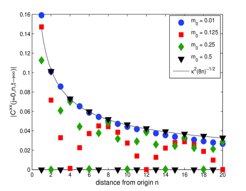
Figure 5: (Color online) Long time behavior of $C^{xx}(j=0,n,t)\,$ for different values of the domain wall height $m_{0}$ defined as $\left\langle\hat{S}^{z}_{j}(t=0)\right\rangle=-sgn(j)m_{0}$. The solid line is the equilibrium correlation function $C^{xx}_{eq}$.

III Quench of a spatially varying magnetic field in a XXZ chain: Bosonization Approach

In this section we will study a general XXZ chain which is subjected to a time-dependent spatially varying magnetic field. The most convenient way to study this problem is via the bosonization approach. We first review some of the notation.

III.1 Equilibrium correlations

The hamiltonian for the $XXZ$-spin chain in a magnetic field is

$$H=\sum_{j}\left[J\left(\hat{S}_{j}^{x}\hat{S}^{x}_{j+1}+\hat{S}_{j}^{y}\hat{S}^{y}_{j+1}\right)+J_{z}\hat{S}_{j}^{z}\hat{S}^{z}_{j+1}-h_{j}S^{z}_{j}\right],$$ (37)

The above can be mapped onto a Luttinger liquid with a back-scattering potential giamarchi ,

$$H=\frac{u}{2\pi}\int dx\left[K(\nabla\theta)^{2}+\frac{1}{K}(\nabla\phi)^{2}\right]$$

$$+\frac{1}{\pi}\int dxh(x)\nabla\phi-\frac{2g}{(2\pi\alpha)^{2}}\int dx\cos(4\phi(x)),$$ (38)

where $g=J_{z}a$, and the fields $\theta\,$ and $\phi\,$ are defined in terms of the boson creation/annihilation operators as

$$\phi(x)=-(N_{R}+N_{L})\frac{\pi x}{L}$$

$$-\frac{i\pi}{L}\sum_{p\neq 0}\left(\frac{L|p|}{2\pi}\right)^{1/2}\frac{1}{p}e^{-\alpha|p|/2-ipx}\left(b_{p}^{\dagger}+b_{-p}\right),$$ (39)

$$\theta(x)=(N_{R}-N_{L})\frac{\pi x}{L}$$

$$+\frac{i\pi}{L}\sum_{p\neq 0}\left(\frac{L|p|}{2\pi}\right)^{1/2}\frac{1}{|p|}e^{-\alpha|p|/2-ipx}\left(b_{p}^{\dagger}-b_{-p}\right).$$ (40)

where $N_{\sigma=R,L}=\sum_{p\neq 0}:\psi_{\sigma}^{\dagger}(p)\psi_{\sigma}(p):$, and $:\cdots:\,$ denotes normal ordering of operators. In the continuum limit, we interpret $x=ja$ for some integer $j$ and lattice spacing $a$. The coupling-parameter relationships are

$$uK = v_{F}=Ja\sin(k_{F}a),$$ (41)

$$\frac{u}{K} = v_{F}\left[1+\frac{2J_{z}a}{\pi v_{F}}\left(1-\cos(2k_{F}a)\right)\right].$$ (42)

For an $xy\,$ anti-ferromagnet ($J>0$), the mapping from spin language to boson language is given by giamarchi

$$\hat{S}^{z}(x) = \frac{-1}{\pi}\nabla\phi(x)+\frac{(-1)^{x}}{\pi\alpha}\cos[2\phi(x)],$$ (43)

$$\hat{S}^{+}(x) = \frac{1}{\sqrt{2\pi\alpha}}\exp[-i\theta(x)]\left[(-1)^{x}+\cos[2\phi(x)]\right].$$ (44)

In equilibrium and zero magnetic fields, the magnetization and basic physical correlations in the gapless anti-ferromagnetic $XX$ phase are

$$\left\langle\hat{S}^{z}(x)\right\rangle=-\frac{1}{\pi}\left\langle\nabla\phi(x)\right\rangle=0,$$ (45)

$$\left\langle\hat{S}^{z}(x+n)\hat{S}^{z}(x)\right\rangle=$$

$$C_{1}\left(\frac{1}{n}\right)^{2}+C_{2}(-1)^{n}\left(\frac{1}{n}\right)^{2K}$$ (46)

$$\left\langle\hat{S}^{+}(x+n)\hat{S}^{-}(x)\right\rangle=$$

$$C_{3}\left(\frac{1}{n}\right)^{2K+\frac{1}{2K}}+C_{4}(-1)^{n}\left(\frac{1}{n}\right)^{\frac{1}{2K}}$$ (47)

where the $C_{j}\,$ are non-universal constants.

The antiferromagnetic Hamiltonian may be transformed to a ferromagnetic Hamiltonian by the transformation $S^{\pm}_{j}\rightarrow(-1)^{j}S^{\pm}_{j}$, resulting in ferromagnetic operators

$$\hat{S}^{z}(x)_{\mbox{\scriptsize f.m.}}=-\frac{1}{\pi}\nabla\phi(x)+\frac{(-1)^{x}}{\pi\alpha}\cos[2\phi(x)],$$ (48)

$$\hat{S}^{+}(x)_{\mbox{\scriptsize f.m.}}=\frac{1}{\sqrt{2\pi\alpha}}\exp[-i\theta(x)]\left[1+(-1)^{x}\cos[2\phi(x)]\right]$$

As a consequence, the magnetization and spin correlations in the gapless ferromagnetic $XX$ phase are,

$$\left\langle\hat{S}^{z}(x)\right\rangle_{\mbox{\scriptsize f.m.}}=-\frac{1}{\pi}\left\langle\nabla\phi(x)\right\rangle=0,$$ (50)

$$\left\langle\hat{S}^{z}(x+n)\hat{S}^{z}(x)\right\rangle_{\mbox{\scriptsize f.m.}}=$$

$$C_{1}\left(\frac{1}{n}\right)^{2}+C_{2}(-1)^{n}\left(\frac{1}{n}\right)^{2K}$$ (51)

$$\left\langle\hat{S}^{+}(x+n)\hat{S}^{-}(x)\right\rangle_{\mbox{\scriptsize f.m.}}=$$

$$C_{3}(-1)^{n}\left(\frac{1}{n}\right)^{2K+\frac{1}{2K}}+C_{4}\left(\frac{1}{n}\right)^{\frac{1}{2K}},$$ (52)

III.2 Magnetic field quench in the XX model ($K=1$)

III.2.1 Diagonalization

In this section we will study the time-dependent Hamiltonian

$$H=H_{i}\theta(-t)+H_{f}\theta(t)$$ (53)

We choose a point in the $XX$ phase corresponding to the $XX$ model $K=1$ and $u=v_{F}$. Thus,

$$H_{i}=\frac{v_{F}}{2\pi}\int dx\left((\nabla\theta)^{2}+(\nabla\phi)^{2}+\frac{2}{v_{F}}h(x)\nabla\phi\right)$$ (54)

$$=\sum_{p\neq 0}v_{F}|p|a_{p}^{\dagger}a_{p},$$ (55)

so that the initial state at $t\leq 0$ is the spatially inhomogeneous ground state of $H_{i}$. The magnetic field $h(x)$ is suddenly switched off at $t=0$ so that the system evolves according to

$$H_{f}=\frac{v_{F}}{2\pi}\int dx\left((\nabla\theta)^{2}+(\nabla\phi)^{2}\right)$$ (56)

$$=\sum_{p\neq 0}v_{F}|p|b_{p}^{\dagger}b_{p}$$ (57)

Since Eq. 54 basically represents harmonic oscillators subjected to an electric field, it may be easily diagonalized by the shift,

$$b_{p}=a_{p}+\lambda_{p}.$$ (58)

where,

$$\lambda_{p}=\frac{1}{v_{F}\sqrt{2\pi|p|L}}h_{p},$$ (59)

and $h_{p}$ is the Fourier transform of $h(x)$. Taking $h(-x)=-h(x)$ (corresponding to a magnetic field that is antisymmetric in space allowing for a domain wall solution), this gives

$$h_{p}=-i\int\sin(px)h(x)dx.$$ (60)

For some time $t$ after the quench, it is straightforward to show that

$$\phi(x,t)=e^{iH_{f}t}\phi(x,0)e^{-iH_{f}t}=\phi^{a}(x,t)+\delta\phi(x,t),$$ (61)

$$\theta(x,t)=e^{iH_{f}t}\theta(x,0)e^{-iH_{f}t}=\theta^{a}(x,t)+\delta\theta(x,t),$$ (62)

where

$$\phi^{a}(x,t)=-\frac{i\pi}{L}\sum_{p\neq 0}\left(\frac{L|p|}{2\pi}\right)^{1/2}$$

$$\times\frac{1}{p}e^{-\alpha|p|/2-ipx}\left(a_{p}^{\dagger}e^{iv_{F}|p|t}+a_{-p}e^{-iv_{F}|p|t}\right),$$ (63)

$$\theta^{a}(x,t)=+\frac{i\pi}{L}\sum_{p\neq 0}\left(\frac{L|p|}{2\pi}\right)^{1/2}$$

$$\times\frac{1}{|p|}e^{-\alpha|p|/2-ipx}\left(a_{p}^{\dagger}e^{iv_{F}|p|t}-a_{-p}e^{-iv_{F}|p|t}\right).$$ (64)

Since we will be computing expectation values with respect to an initial state which is the ground state of the $a_{p}$ operators, $\phi^{a},\theta^{a}$ will just return the equilibrium results. Thus the effect of the shift and hence the initial magnetic field is contained entirely in

$$\delta\phi(x,t) = \frac{i}{\pi v_{F}}\int_{0}^{\infty}\frac{dp}{p}\cos[pv_{F}t]\cos[px]h_{p},$$ (65)

$$\delta\theta(x,t) = \frac{-i}{\pi v_{F}}\int_{0}^{\infty}\frac{dp}{p}\sin[pv_{F}t]\sin[px]h_{p}.$$ (66)

For any antisymmetric $h(x)$ the above reduces to,

$$\delta\phi(x,t)=\frac{1}{8v_{F}}\int_{-\infty}^{\infty}dx^{\prime}h(x^{\prime})\left[\mbox{sgn}[x^{\prime}+z_{-}]\right.$$

$$\left.+\mbox{sgn}[x^{\prime}+z_{+}]+\mbox{sgn}[x^{\prime}-z_{+}]+\mbox{sgn}[x^{\prime}-z_{-}]\right],$$ (67)

$$\delta\theta(x,t)=\frac{1}{8v_{F}}\int_{-\infty}^{\infty}dx^{\prime}h(x^{\prime})\left[\mbox{sgn}[x^{\prime}+z_{+}]\right.$$

$$\left.+\mbox{sgn}[x^{\prime}-z_{+}]-\mbox{sgn}[x^{\prime}+z_{-}]-\mbox{sgn}[x^{\prime}-z_{-}]\right],$$ (68)

where $\mbox{sgn}[x]\equiv x/|x|$, and $z_{\pm}=x\pm v_{F}t$.

The above implies that the magnetization before the quench is

$$\left\langle\hat{S}^{z}\right\rangle=-\frac{1}{\pi}\langle\frac{\partial\phi(x)}{\partial x}\rangle=-\frac{1}{\pi}\frac{\partial\delta\phi(x)}{\partial x}=\frac{1}{\pi v_{F}}h(x)$$ (69)

Thus within the bosonization approach, the magnetization follows the magnetic-field profile.

III.2.2 Magnetization and Correlations after the quench

The magnetization at some time $t$ after the magnetic-field quench is

$$\left\langle\hat{S}^{z}\right\rangle=-\frac{1}{\pi}\left\langle\partial_{x}\phi^{a}(x,t)\right\rangle-\frac{1}{\pi}\partial_{x}\delta\phi(x,t)$$

$$=\frac{1}{2\pi v_{F}}\left(h(x+v_{F}t)+h(x-v_{F}t)\right)$$ (70)

As anticipated, the domain wall spreads out with speed $v_{F}$ in both directions. This result is consistent with the ballistic time-evolution found in section II from the exact solution of the fermionic problem.

Next we turn to the evaluation of the $C^{xx}$ correlation function which from the exact solution of the fermionic model was found to be $\left\langle\hat{S}^{x}_{j+n}\hat{S}^{x}_{j}\right\rangle\rightarrow\cos\left(\frac{2\pi n}{\lambda}\right)C^{xx}_{eq}(n)$ where $C^{xx}_{eq}(n)\sim\frac{1}{\sqrt{n}}$ was the equilibrium correlation function, and the wavelength of the oscillation was found to be $\lambda=\frac{2}{m_{0}}$, $m_{0}$ being the height of the domain wall (or the magnitude of the maximal magnetization at the ends of the domain wall).

In the bosonization approach,

$$\left\langle\hat{S}^{+}(x+n,t)\hat{S}^{-}(x,t)\right\rangle\sim$$

$$\exp[-i(\delta\theta(x+n,t)-\delta\theta(x,t))]\frac{1}{\sqrt{n}}.$$ (71)

Let us suppose

$$h(x)=h_{0}\tanh(x/\xi)$$ (72)

implying

$$h_{p}=-ih_{0}\left(\frac{\pi\xi}{\sinh\left(\frac{\pi p\xi}{2}\right)}\right)$$ (73)

Then we find,

$$\delta\theta(x+n,t)-\delta\theta(x,t)=$$

$$-\frac{\xi h_{0}}{2v_{F}}\log\left[\frac{\cosh[(x-v_{F}t)/\xi]\cosh[(x+n+v_{F}t)/\xi]}{\cosh[(x+n-v_{F}t)/\xi]\cosh[(x+v_{F}t)/\xi]}\right]$$

$$\xrightarrow{v_{F}t,|v_{F}t\pm x|,|v_{F}t\pm(x+n)|\gg\xi}-\frac{\xi h_{0}}{2v_{F}}\left[\frac{|x-v_{F}t|}{\xi}\right.$$

$$\left.+\frac{|x+n+v_{F}t|}{\xi}-\frac{|x+n-v_{F}t|}{\xi}-\frac{|x+v_{F}t|}{\xi}\right]$$ (74)

For $v_{F}t>>|x|,|x+n|$, i.e, long after the moving domain wall front has crossed the two observation points at $x$ and $x+n$, we find

$$\delta\theta(x+n,t)-\delta\theta(x,t)\rightarrow\frac{h_{0}n}{v_{F}}.$$ (75)

so that

$$\left\langle\hat{S}^{+}(x+{n})\hat{S}^{-}(x)\right\rangle\sim e^{i{n}h_{0}/v_{F}}\left(\frac{1}{\sqrt{n}}\right).$$ (76)

Thus we find that for an initial domain wall that has the profile

$$\left\langle S^{z}(x=\pm\infty)\right\rangle\longrightarrow\pm\frac{h_{0}}{\pi v_{F}}=\pm m_{0}$$ (77)

the transverse spin correlation function at long times do not equilibrate but acquire a spatial oscillation at the wavelength

$$\lambda=\frac{2\pi v_{F}}{h_{0}}=\frac{2}{m_{0}}$$ (78)

This result is identical to that obtained from the exact solution of the fermionic problem (Eqns. 34, 36).

Note that the wavelength of the spatial oscillation is set by the height of the domain wall $m_{0}$ and is independent of the width $\xi$ (or $\alpha=\frac{J}{{\cal F}a}$ in the fermionic problem). For the case of a linearly varying magnetic field studied in the previous section, the domain wall magnetization approached its maximum possible value $\mp\frac{1}{2}\,$ at its two ends. This in the boson language corresponds to

$$\frac{h_{0}}{v_{F}}\rightarrow-\frac{\pi}{2a},$$ (79)

so that writing $n=\bar{n}a$ in Eq. 76, where $\bar{n}$ is an integer,

$$\left\langle S^{+}(x+\bar{n}a)S^{-}(x)\right\rangle\rightarrow e^{i\pi\bar{n}/2}\left(\frac{1}{\sqrt{\bar{n}}}\right),$$ (80)

giving us precisely the observed behavior of Eq. 32.

For the evaluation of the $\langle S^{z}S^{z}\rangle$ correlation function, we need to evaluate $\exp\left[i\delta\phi(x+n,t)-i\delta\phi(x,t)\right]$. We find,

$$\delta\phi(x+n,t)-\delta\phi(x,t)=$$

$$\frac{-h_{0}\xi}{2v_{F}}\log\left[\frac{\cosh\left[\frac{x+n+v_{F}t}{\xi}\right]\cosh\left[\frac{x+n-v_{F}t}{\xi}\right]}{\cosh\left[\frac{x+v_{F}t}{\xi}\right]\cosh\left[\frac{x-v_{F}t}{\xi}\right]}\right]$$ (81)

$$\xrightarrow{v_{F}t\gg\xi,|x|,|x+n|}0$$

The above result together with the fact that

$$\partial_{x}\delta\phi(x+n,t)\partial_{x}\delta\phi(x,t)=$$

$$\frac{1}{4\pi v_{F}^{2}}\left(h(x+v_{F}t)+h(x-v_{F}t)\right)$$

$$\times\left(h(x+n+v_{F}t)+h(x+n-v_{F}t)\right).$$ (82)

implies that for $v_{F}t\gg\xi,|x|,|x+n|$, the $C^{zz}$ correlation function equilibrates which is in agreement with the results in section II.

To summarize the results of this section: a). Within the bosonization approach, an applied magnetic-field produces a spin pattern that follows the local magnetic field. b). After a quench, the domain wall spreads out ballistically. The magnetization equilibrates (in this case vanishes to zero everywhere). c). The $C^{zz}$ correlation function equilibrates, whereas the $C^{xx}$ correlation function acquires spatial oscillations at wavelength $\lambda=\frac{2}{m_{0}}$ where $m_{0}$ is the height of the initial domain wall defined as $S_{z}(\pm\infty)=\pm m_{0}$. These results are in agreement with the exact results of section II obtained from solving the fermion lattice problem. Thus bosonization is good at capturing the behavior at long distances and times, even for the nonequilibrium problem. As expected it misses some of the details of the short distance physics both in the static properties (as shown in Fig. 6), as well as during the time-evolution such as the existence of a complex internal structure in the propagating domain wall front Hunyadi04 .

Figure 6: (Color online) Plot of the magnetization obtained from the bosonization approach with $h(x)=h_{0}\tanh{x/\xi}$, and from the fermionic lattice model with $\alpha=20$.

In the next section we provide an explanation for the inhomogeneities observed in the transverse spin correlation function by solving the classical equations of motion for the spins.

IV Magnetic field quench in a classical $XX$ spin chain: Formation of a transverse spin-wave pattern

The Hamiltonian in Eq. 1 implies the following equations of motion for the spins

$$\frac{dS^{z}_{j}}{dt}=-J\left[S^{y}_{j}\left(S^{x}_{j+1}+S^{x}_{j-1}\right)-S^{x}_{j}\left(S^{y}_{j+1}+S^{y}_{j-1}\right)\right]$$

(83)

$$\frac{dS^{x}_{j}}{dt}=-JS^{z}_{j}\left(S^{y}_{j+1}+S^{y}_{j-1}\right)-h_{j}S^{y}_{j}$$ (84)

$$\frac{dS^{y}_{j}}{dt}=JS^{z}_{j}\left(S^{x}_{j+1}+S^{x}_{j-1}\right)+h_{j}S^{x}_{j}$$ (85)

We will treat the spins as classical variables, and solve the above equations for a sudden quench of a spatially inhomogeneous magnetic field, $h_{j}(t)=h_{j}\theta(-t)$. First notice that for $t\leq 0$, after performing the course-graining $S^{a}_{j}=S^{a}_{j+1}$, the following spin profile satisfy the equations of motion,

$$S^{z}_{j}=-\frac{h_{j}}{2J}$$ (86)

$$S^{x}_{j}=\sqrt{S^{2}-(S^{z}_{j})^{2}}$$ (87)

$$S^{y}_{j}=0$$ (88)

With the above as an initial condition, the dynamics for $t>0$ can be easily studied numerically and we find a ballistic spreading out of the domain wall profile (see Fig. 7), and the appearance of a spin-wave pattern. The latter result, i.e., the appearance of an inhomogeneous pattern at long times can be verified analytically rather easily as follows. Suppose, $h_{j}(t)=-h_{0}\tanh\frac{x}{\xi}\theta(-t)$. Then for $t>0$, if we assume a ballistic broadening of the domain wall,

$$S^{z}_{j}(t)=\frac{h_{0}}{2J}\left[\tanh(\frac{ja-vt}{\xi})+\tanh(\frac{ja+vt}{\xi})\right]$$ (89)

Writing Eq. 84, 85 in terms of $S^{\pm}=S^{x}\pm iS^{y}$, and performing a course-graining, one obtains the following equation for $S^{+}(x=ja)$

$$\frac{dS^{+}(x,t)}{dt}=2iJS^{z}(x,t)S^{+}(x,t)$$ (90)

Using Eq. 89, Eq. 90 may be easily solved to obtain

$$S^{+}(x,t)=S^{+}(x,0)\exp\left[\frac{ih_{0}\xi}{2v}\left(\ln\frac{\cosh(\frac{vt+x}{\xi}}{\cosh(\frac{vt-x}{\xi}}\right)\right]$$ (91)

Thus for $vt\gg|x|$ we find the spin-wave pattern

$$S^{+}(x,t)\rightarrow S^{+}(x,0)e^{ih_{0}x/v}$$ (92)

in agreement with the results of the previous sections.

Thus the appearance of the spatial inhomogeneity may be understood as follows. Right after the magnetic field is switched off, the spins in the XY plane begin to precess due to a non-zero magnetization in the z-direction. However this precession only lasts for as long as it takes the domain wall profile to flatten out to zero. Since this time is different for spins located at different spatial positions, the spins locally dephase with respect to each other and arrange themselves in a spin-wave pattern.

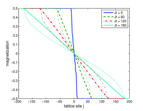
Figure 7: (Color online) Thick line: Time evolution of the magnetization from the solution of the classical Landau-Lifshitz equation assuming that $S_{z}(t\leq 0)$ is given by Eq. 9. Thin lines: Time evolution from the exact solution of the quantum problem.

V Quench of a spatially varying magnetic field and interactions in a XXZ chain: Bosonization Approach

V.1 Quench within the gapless XX phase

We will now turn our attention to the case where as the magnetic field is switched off at $t=0$, the interactions are also turned on so that the Luttinger parameter is $K=\theta(-t)+K\theta(t)$. We will first consider the case where the ground state both before and after the quench corresponds to a gapless XX phase, so that the $\cos(\beta\phi)$ term can be neglected.

V.1.1 Bogoliubov rotation

We wish to begin with a non-interacting system in an inhomogeneous magnetic field,

$$H_{i}=\frac{v_{F}}{2\pi}\int dx\left((\nabla\phi)^{2}+(\nabla\theta)^{2}+\frac{2}{v_{F}}h(x)\nabla\phi\right)$$ (93)

$$=\sum_{p\neq 0}v_{F}|p|a_{p}^{\dagger}a_{p},$$ (94)

and quench to zero field, while turning on interactions so that

$$H_{f}=\frac{u}{2\pi}\int dx\left(\frac{1}{K}(\nabla\phi)^{2}+K(\nabla\theta)^{2}\right)$$ (95)

$$=\sum_{p\neq 0}u|p|\eta_{p}^{\dagger}\eta_{p}.$$ (96)

The $\eta_{p}\,$ operators have a simple time evolution and may be related to the $b_{p}\,$ operators by a Bogoliubov rotation cazalilla1 ; cazalilla ,

$$\eta_{p} = \cosh\beta b_{p}+\sinh\beta b_{-p}^{\dagger},$$ (97)

$$\eta_{p}^{\dagger} = \cosh\beta b_{p}^{\dagger}+\sinh\beta b_{-p}.$$ (98)

where $e^{-2\beta}=K$. We define,

$$f(p,t) = \cos(u|p|t)-i\sin(u|p|t)\cosh(2\beta),$$ (99)

$$g(p,t) = i\sin(u|p|t)\sinh(2\beta).$$ (100)

and $\alpha_{\pm}\equiv f(p,t)\pm g(p,t)$. Performing the shift $b_{p}=a_{p}+\lambda_{p}$ as before, we write the $\phi$ and $\theta$ fields as $(\phi,\theta)=(\phi_{\beta}^{a},\theta_{\beta}^{a})+\delta(\phi_{\beta},\theta_{\beta})$, where

$$\phi_{\beta}^{a}(x,t)=\frac{-i\pi}{L}\sum_{p\neq 0}\left(\frac{L|p|}{2\pi}\right)^{1/2}\frac{1}{p}e^{-\alpha|p|/2-ipx}\left(\alpha_{+}^{*}a_{p}^{\dagger}\right.$$

$$\left.+\alpha_{+}a_{-p}\right)$$ (101)

$$\theta_{\beta}^{a}(x,t)=\frac{i\pi}{L}\sum_{p\neq 0}\left(\frac{L|p|}{2\pi}\right)^{1/2}\frac{1}{|p|}e^{-\alpha|p|/2-ipx}\left(\alpha_{-}^{*}a_{p}^{\dagger}\right.$$

$$\left.-\alpha_{-}a_{-p}\right),$$ (102)

The $\delta(\phi,\theta)$ arise due to the spatially varying magnetic field and are given by,

$$\delta\phi_{\beta}(x,t) = \frac{u}{v_{F}}\delta\phi(x,t,\beta=0,v_{F}\rightarrow u),$$ (103)

$$\delta\theta_{\beta}(x,t) = \frac{ue^{2\beta}}{v_{F}}\delta\theta(x,t,\beta=0,v_{F}\rightarrow u),$$ (104)

where $\delta\phi(x,t,\beta=0,v_{F}),\delta\theta(x,t,\beta=0,v_{F})$ are given in Eq. 65 and 66 respectively.

V.1.2 Magnetization after the quench

It is straightforward to show that the magnetization at a time $t$ after the quench is

$$S_{z}(x,t)=-\frac{1}{\pi}\frac{\partial\delta\phi(x)}{\partial x}=\frac{1}{2\pi v_{F}}\left[h(x+ut)+h(x-ut)\right]$$

Thus even with the interaction quench, the domain wall spreads out ballistically, but with the renormalized velocity $u=v_{F}/K$.

V.1.3 Basic non-equilibrium correlations

To compute the correlation functions, some basic expressions we need are

$$G_{\phi\phi}=\left\langle[\phi^{a}_{\beta}(x,t)-\phi^{a}_{\beta}(x^{\prime},t)]^{2}\right\rangle$$ (106)

$$G_{\theta\theta}=\left\langle[\theta^{a}_{\beta}(x,t)-\theta^{a}_{\beta}(x^{\prime},t)]^{2}\right\rangle$$ (107)

Note that $G_{\theta\theta}\,$ is related to $G_{\phi\phi}$ by $K\rightarrow\frac{1}{K}$ the computation of which is identical to that already presented in cazalilla1 ; cazalilla . For completeness we present the results below,

$$G_{\phi\phi}=\int_{0}^{\infty}\frac{dp}{p}\left[\cos^{2}(utp)+e^{-4\beta}\sin^{2}(utp)\right]$$

$$\times(1-\cos[p(x-x^{\prime})])e^{-\alpha p}$$ (108)

which eventually gives

$$G_{\phi\phi}=G_{\phi\phi}^{(0)}+\left(\frac{K^{2}-1}{8}\right)\times$$

$$\log\left[\frac{[\alpha^{2}+(2ut)^{2}]^{2}[\alpha^{2}+x^{2}]^{2}}{\alpha^{4}[\alpha^{2}+(2ut+x)^{2}][\alpha^{2}+(x-2ut)^{2}]}\right]$$ (109)

$$G_{\theta\theta}=G_{\theta\theta}^{(0)}+\left(\frac{K^{-2}-1}{8}\right)\times$$

$$\log\left[\frac{[\alpha^{2}+(2ut)^{2}]^{2}[\alpha^{2}+x^{2}]^{2}}{\alpha^{4}[\alpha^{2}+(2ut+x)^{2}][\alpha^{2}+(x-2ut)^{2}]}\right].$$ (110)

where $G_{\phi\phi}^{(0)}=\frac{K}{2}\log\left[\frac{x^{2}+\alpha^{2}}{\alpha^{2}}\right]$, $G_{\theta\theta}^{(0)}=\frac{1}{2K}\log\left[\frac{x^{2}+\alpha^{2}}{\alpha^{2}}\right]$.

V.1.4 Spin correlations after the quench

Taking the $2ut>>x\,$ limit, we can easily obtain the correlator asymptotics. The memory of the initial domain wall profile appears as oscillatory pre-factors of the form $\exp[2i(\delta\phi(x+n)-\delta\phi(x))]$ and terms such as $\nabla\delta\phi(x+n)\nabla\delta\phi(x)$. For the specific case of $h(x)=h_{0}\tanh(x/\xi)$ we find at long times,

$$\left\langle\hat{S}^{z}(x+n)\hat{S}^{z}(x)\right\rangle=f(x+n,t)f(x,t)$$

$$+\frac{C^{\prime}_{1}}{n^{2}}+\frac{C^{\prime}_{2}(-1)^{n}}{n^{K^{2}+1}}$$ (111)

$$\left\langle\hat{S}^{+}(x+n)\hat{S}^{-}(x)\right\rangle=\frac{C^{\prime}_{3}e^{\frac{ih_{0}n}{v_{F}K}}}{n^{1+K^{2}+\frac{1+K^{-2}}{4}}}$$

$$+\frac{C^{\prime}_{4}(-1)^{n}e^{\frac{ih_{0}n}{v_{F}K}}}{n^{\frac{1+K^{-2}}{4}}}$$ (112)

where

$$f(x,t)=\frac{1}{2v_{F}}\left(h(x+ut)+h(x-ut)\right)$$ (113)

The case of the pure interaction quench ($h_{0}=0$) was studied in cazalilla1 ; cazalilla where the above anomalous power-laws corresponding to an algebraic decay which is faster than in equilibrium (since $K^{2}+1\geq 2K\,$ for all real $K$) were obtained. From Eq. 112 we find that the effect of an initial domain wall profile is to superimpose spatial oscillations onto this decay, where the wavelength of the oscillations depends on the interaction parameter $K$ and is found to be

$$\lambda=\frac{2\pi v_{F}K}{h_{0}}=\frac{2K}{m_{0}}$$ (114)

As expected, increasing the exchange interaction $J_{z}$ increases the effective magnetic field seen by the precessing spins, thus decreasing the wave-length of the spin wave pattern.

V.1.5 Generalized Gibbs Ensemble

Rigol et al have made the interesting proposal that the long-time properties of out of equilibrium integrable systems may be captured by a generalized Gibbs ensemble that enforces the constraints imposed by the integrals of motion rigol07 . This approach has been applied with success by Iucci and Cazalilla cazalilla1 ; cazalilla who studied homogeneous interaction quenches in models similar to those studied in this paper. It has also been successfully applied to models of free bosons Cardy07 , and for some general family of integrable models Mussardo09 . An interesting question has been to identify situations in which the Gibbs ensemble argument might break down Barthel08 ; Biroli09 . We find that for an inhomogeneous quantum quench starting from an initial domain wall state, the Gibbs ensemble argument cannot capture the spatial inhomogeneities at long times after the quench. In this section we review the Gibbs ensemble argument and show why this does not work for our case.

Consider a quantum quench of the form $H=H_{i}\theta(-t)+H_{f}\theta(t)$, so that for $t\leq 0$ the system is in the ground state of $H_{i}$, whereas at $t>0$, the wave-function begins to evolve according to $H_{f}$. Let us further assume that both $H_{i}$ and $H_{f}$ can be diagonalized

$$H_{i}=\sum_{p}\epsilon^{a}_{p}a_{p}^{\dagger}a_{p}$$ (115)

$$H_{f}=\sum_{p}\epsilon^{b}_{p}b_{p}^{\dagger}b_{p}$$ (116)

and that the two Hilbert spaces may be related to each other via a canonical transformation. For the case of bosons a general canonical transformation is of the form,

$$b_{p}=\cosh\Theta_{p}a_{p}+\sinh\Theta_{p}a_{-p}^{\dagger}+\lambda_{p}$$ (117)

where $\lambda_{p}$ is a linear shift and $\Theta_{p}$ is a rotation angle .

The essential idea behind predicting the long-time behavior is that an integrable model such as $H_{f}$ has a conserved quantity for every degree of freedom. For the example given above, the conserved quantity is trivially given by $I_{p}=b_{p}^{\dagger}b_{p}$. Thus during the time-evolution $\langle b^{\dagger}_{p}b_{p}\rangle$ should be conserved. Since the initial state is the ground state of $H_{i}$ for which $\left\langle a_{p}^{\dagger}a_{p}\right\rangle=0\,$ for $p\neq 0$, it follows that the Gibbs’ ensemble should be characterized by the distribution function

$$\left\langle b_{p}^{\dagger}b_{p}\right\rangle=|\lambda_{p}|^{2}+\sinh^{2}\Theta_{p}.$$ (118)

For the particular models studied here, we find the initial spatial inhomogeneity is captured by the linear shift $\lambda_{p}$ (given by Eq. 59), while the angle $\Theta_{p}$ captures the homogeneous changes in the interaction parameter. Since in our example $|\lambda_{p}|^{2}$ vanishes in the thermodynamic limit, any effect of the initial spatial inhomogeneity is lost. Thus while the Gibbs ensemble captures the effect of the rotation, and therefore correctly predicts the new power law exponents of cazalilla1 , it misses the spin-wave pattern at long times. In particular the Gibbs ensemble prediction for the transverse spin correlation function is given by

$$\left\langle\hat{S}^{+}(x+n)\hat{S}^{-}(x)\right\rangle=\frac{C^{\prime}_{3}}{n^{1+K^{2}+\frac{1+K^{-2}}{4}}}$$

$$+\frac{C^{\prime}_{4}(-1)^{n}}{n^{\frac{1+K^{-2}}{4}}}$$ (119)

which differs from the correct answer (Eq. 112) by the absence of the spatially oscillating factors $e^{\frac{ih_{0}n}{v_{F}K}}$.

V.2 Magnetic field and Interaction quench into the gapped Ising phase: Semiclassical treatment

In this section we will study the effect of quenching the external magnetic field and the interactions into the massive Ising phase where the $\cos\phi$ term is strongly relevant. In order to study the time evolution, we will employ a semi-classical approximation which corresponds to replacing $\cos\phi\sim 1-\frac{\phi^{2}}{2}$. Thus for this case the initial wave-function is the ground state of

$$H_{i} = \frac{v_{F}}{2\pi}\int dx\left[(\nabla\phi)^{2}+(\nabla\theta)^{2}+\frac{2}{v_{F}}h(x)\nabla\phi\right],$$ (120)

$$= \sum_{p}v_{F}|p|a_{p}^{\dagger}a_{p}$$ (121)

while for $t>0$ the wave-function evolves according to

$$H_{f} = \frac{u}{2\pi}\int dx\left[(\nabla\tilde{\phi})^{2}+(\nabla\tilde{\theta})^{2}+\frac{m^{2}}{u^{2}}\tilde{\phi}^{2}\right]$$ (122)

$$= \sum_{p}\omega_{p}\eta_{p}^{\dagger}\eta_{p}$$ (123)

where $\tilde{\phi}=\frac{\phi}{\sqrt{K}},\tilde{\theta}=\sqrt{K}\theta$ and $\omega_{p}=\sqrt{p^{2}u^{2}+m^{2}}$.

The calculations mirror that of the previous section. Writing $\phi=\phi^{a}+\delta\phi,\theta=\theta^{a}+\delta\theta$, we find for a time $t$ after the quench

$$\phi^{a}(x,t)=-\frac{i\pi}{L}\sum_{p\neq 0}\left(\frac{L|p|}{2\pi}\right)^{1/2}$$

$$\times\frac{1}{p}e^{-\alpha|p|/2-ipx}\left[a_{p}^{\dagger}\left(\cos(\omega_{p}t)+iK\frac{u|p|}{\omega_{p}}\sin(\omega_{p}t)\right)\right.$$

$$\left.+a_{-p}\left(\cos(\omega_{p}t)-iK\frac{u|p|}{\omega_{p}}\sin(\omega_{p}t)\right)\right],$$ (124)

$$\theta^{a}(x,t)=\frac{i\pi}{L}\sum_{p\neq 0}\left(\frac{L|p|}{2\pi}\right)^{1/2}$$

$$\times\frac{1}{|p|}e^{-\alpha|p|/2-ipx}\left[a_{p}^{\dagger}\left(\cos(\omega_{p}t)+i\frac{\omega_{p}}{Ku|p|}\sin(\omega_{p}t)\right)\right.$$

$$\left.-a_{-p}\left(\cos(\omega_{p}t)-i\frac{\omega_{p}}{Ku|p|}\sin(\omega_{p}t)\right)\right]$$ (125)

and

$$\delta\phi(x,t) = \frac{i}{\pi v_{F}}\int_{0}^{\infty}\frac{dp}{p}\cos[\omega_{p}t]\cos[px]h_{p},$$ (126)

$$\delta\theta(x,t) = \frac{-i}{\pi Kv_{F}}\int_{0}^{\infty}\frac{dp}{p}\sin[\omega_{p}t]\sin[px]\left(\frac{\omega_{p}}{u|p|}\right)h_{p}$$

V.2.1 Magnetization after the quench

The magnetization at a time $t$ after the quench is given by $\langle S^{z}(x,t)\rangle=-\frac{1}{\pi}\partial_{x}\phi(x,t)+\frac{(-1)^{x}}{\pi\alpha}\langle\cos(2\phi(x,t))\rangle$. Due to the presence of infra-red divergences, we find that for all times after the quench,

$$\left\langle e^{-2i\phi(x,t)}\right\rangle\sim 0$$ (128)

so that Ising order never develops. This is consistent with the results of cazalilla and may be an artifact of the semi-classical approximation. In section VI we will compare this result with a mean-field treatment for the order-parameter dynamics.

Thus, within the validity of the semiclassical approximation we find the following time evolution for the initial domain wall profile,

$$\left\langle S^{z}(x,t)\right\rangle=-\frac{1}{\pi}\partial_{x}\left(\delta\phi(x,t)\right)$$

$$=\frac{h_{0}}{\pi v_{F}}\int_{0}^{\infty}dz\cos\left(\frac{ut}{\xi}\sqrt{z^{2}+\left(\frac{m\xi}{u}\right)^{2}}\right)$$

$$\times\frac{\sin\left(\frac{x}{\xi}z\right)}{\sinh\left(\frac{\pi z}{2}\right)}$$ (129)

The above is plotted in Fig. 8 for several different masses. The domain wall profile shows a more complex time evolution than for the quench in the gapless phase where a simple ballistic broadening of the domain wall occurs. In the Ising phase instead we find oscillations of the local magnetization at the frequency of the mass. In addition the domain wall spreads out less and less as the mass increases, a result which is in agreement with a t-DMRG study of the XXZ chain tdmrg05 ; tdmrg09 . Note however that we find oscillations of the magnetization outside the light-cone at the time-scale of $1/m$. This is due to the nature of the Klein-Gordon equation $\partial_{t}^{2}-\partial_{x}^{2}+m^{2}$ which has solutions of the form $e^{ikx-i\sqrt{k^{2}+m^{2}}t}\xrightarrow{mt\gg 1}e^{-imt}e^{ikx-i\frac{k^{2}}{2m}t}$. The t-DMRG results on the other hand found oscillations only within the light cone.

We also find that the magnetization eventually equilibrates at long times. Fig. 9 shows the time evolution for the magnetization for a given point in position space. At long times Eq. 129 may be evaluated in a stationary phase approximation which gives,

$$\langle S^{z}(x,t)\rangle\simeq\frac{2h_{0}x}{\pi v_{F}}\sqrt{\frac{2m}{\pi u^{2}t}}\cos\left(mt+\frac{\pi}{4}\right)$$ (130)

showing that the magnetization decays locally as a power-law.

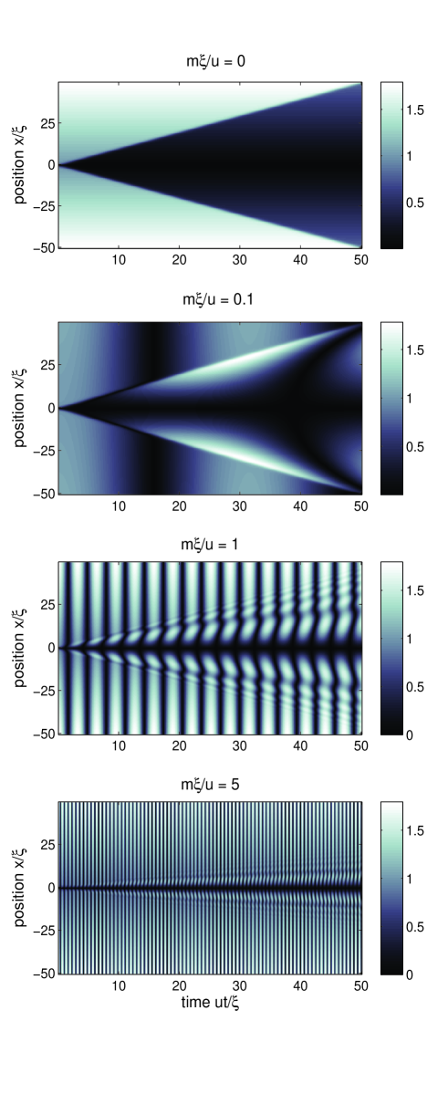
Figure 8: Contour plot for $|S_{z}|$ after a “semi-classical” quench for several different masses.

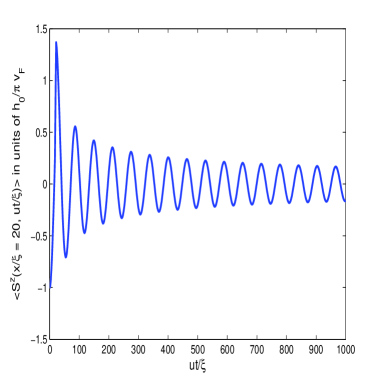
Figure 9: (Color online) The magnetization decays as $t^{-1/2}\,$ with oscillations of period $\sim m^{-1}$. Here, $m\xi/u=0.1$.

V.2.2 Correlation functions after the quench

Here we give results for some typical spin correlation functions. Again, due to the presence of infra-red divergences, the transverse-spin correlation function is found to vanish at all times after the quench,

$$\langle e^{i\theta(x,t)}e^{-i\theta(0,t)}\rangle\sim 0$$ (131)

On the other hand the $z-z$ correlation function is found to be

$$\left\langle e^{2i\phi(x,t)}e^{-2i\phi(0,t)}\right\rangle=e^{2i(\delta\phi(x,t)-\delta\phi(x,0))}A^{\prime}(\alpha)\left(\frac{1}{x}\right)$$ (132)

For a purely interaction quench ($\delta\phi=0$) we find a power law decay in the Ising phase with an exponent which is half of that in the initial gapless phase, a result which was also found by cazalilla for homogeneous quenches. The initial domain profile superimposes the additional structure

$$e^{2i(\delta\phi(x,t)-\delta\phi(y,0))}\xrightarrow{mt\gg 1}e^{2i\left[\frac{h_{0}(x^{2}-y^{2})}{v_{F}}\sqrt{\frac{2m}{\pi u^{2}t}}\cos\left(mt+\frac{\pi}{4}\right)\right]}$$ (133)

Thus at long times, the spatial oscillations due to the initial domain-wall eventually decay to zero.

VI Effect of quenching a magnetic field and interactions: Mean-field treatment

In this section we will use a mean-field argument to explore whether after quenching both a magnetic field as well as interactions, local anti-ferromagnetic (AF) Ising order can develop. Thus our initial wave-function corresponds to the ground state of the following Hamiltonian

$$H_{i}=J\sum_{j}\left[S_{j}^{x}S_{j+1}^{x}+S_{j}^{y}S_{j+1}^{y}+\frac{h_{j}}{J}S_{j}^{z}\right]$$ (134)

with $J>0$, and we will assume $h_{j}={\cal F}ja$. While, as a result of the quench the wave-function evolves in time due to

$$H_{f}=J\sum_{j}\left(S_{j}^{x}S_{j+1}^{x}+S_{j}^{y}S_{j+1}^{y}\right)+J^{z}\sum_{j}S_{j}^{z}S_{j+1}^{z}$$ (135)

Performing a Jordan-Wigner transformation followed by the change of variables $c_{i}\rightarrow(-1)^{i}c_{i}$, $H_{i}$ becomes identical to the Hamiltonian (Eq. 2) already studied in section II.1, whereas the Hamiltonian after the quench is,

$$H_{f}=-\frac{J}{2}\sum_{i}\left(c_{i}^{\dagger}c_{i+1}+h.c.\right)$$

$$+J^{z}\sum_{i}\left(c_{i}^{\dagger}c_{i}-\frac{1}{2}\right)\left(c_{i+1}^{\dagger}c_{i+1}-\frac{1}{2}\right)$$ (136)

Thus the initial state which is the ground state of $H_{i}$ (given by Eq. 7) evolves in time according to Eq. 136. In what follows we will study this time evolution using a mean-field approximation.

Defining the AF order-parameter at a time $t$, $\Delta_{0}(t)$ as $\langle c_{i}^{\dagger}(t)c_{i}(t)\rangle=\frac{1}{2}+(-1)^{i}\Delta_{0}(t)$, Eq. 136 within a mean-field approximation becomes

$$H_{f}^{mf}=\sum_{|k|<\pi/2}\epsilon_{k}\left(c_{k}^{\dagger}c_{k}-c^{\dagger}_{k+\pi}c_{k+\pi}\right)$$

$$-2J^{z}\Delta_{0}(t)\sum_{|k|<\pi/2}\left(c_{k}^{\dagger}c_{k+\pi}+c_{k+\pi}^{\dagger}c_{k}\right)$$ (137)

where $\epsilon_{k}=-J\cos{ka}$, and $\Delta_{0}(t)$ is determined from the self-consistency condition

$$\Delta_{0}(t)=\frac{1}{N}\langle\Psi|e^{iH^{mf}_{f}t}\sum_{i}(-1)^{i}c_{i}^{\dagger}c_{i}e^{-iH^{mf}_{f}t}|\Psi\rangle$$ (138)

where $N$ is the total number of sites.

In terms of the amplitudes $\tilde{c}_{k\pm}$ of being in the adiabatic eigenstates of $H^{mf}_{f}$, the self-consistency condition becomes

$$\Delta_{0}(t)=\frac{1}{2N}\sum_{|k|<\pi/2}\left[\sin 2\theta_{k}(t)\left(|\tilde{c}_{k+}(t)|^{2}-|\tilde{c}_{k-}(t)|^{2}\right)\right.$$

$$\left.-\cos 2\theta_{k}(t)\left(\tilde{c}_{k+}^{*}(t)\tilde{c}_{k-}(t)+\tilde{c}_{k-}^{*}(t)\tilde{c}_{k+}(t)\right)\times\right.$$

$$\left.\cos(\int_{0}^{t}dx(E_{k+}(x)-E_{k-}(x)))\right.$$

$$\left.-i\cos 2\theta_{k}(t)\left(\tilde{c}_{k+}^{*}(t)\tilde{c}_{k-}(t)-\tilde{c}_{k-}^{*}(t)\tilde{c}_{k+}(t)\right)\times\right.$$

$$\left.\sin(\int_{0}^{t}dx(E_{k+}(x)-E_{k-}(x)))\right]$$ (139)

where

$$E_{k\pm}(t)=\pm\sqrt{\epsilon_{k}^{2}+4J_{z}^{2}\Delta_{0}^{2}(t)}$$ (140)

$$\tan{2\theta_{k}}(t)=-\frac{2J_{z}\Delta_{0}(t)}{\epsilon_{k}}$$ (141)

and the coefficients $\tilde{c}_{k\pm}$ satisfy the equations of motion,

$$\frac{d\tilde{c}_{k\pm}(t)}{dt}=\tilde{c}_{k\mp}(t)\left[\frac{\pm\epsilon_{k}J_{z}\frac{d\Delta_{0}}{dt}}{\epsilon_{k}^{2}+4J_{z}^{2}\Delta_{0}^{2}}\right]e^{\pm i\int_{0}^{t}dx(E_{k+}(x)-E_{k-}(x))}$$

In an adiabatic approximation $\frac{\dot{\Delta}_{0}}{\Delta^{2}_{0}}\ll 1$, we can approximate $\tilde{c}_{k\pm}$ by its value at $t=0$. In this case Eq. 139 becomes

$$\Delta_{0}\simeq\frac{1}{2N}\sum_{|k|<\pi/2}\left[\sin 2\theta_{k}(t)\left(\sin{2\theta_{k}}(t)I_{k}^{x}+\cos{2\theta_{k}}(t)I_{k}^{z}\right)\right.$$

$$\left.-\cos 2\theta_{k}(t)\left(\sin{2\theta_{k}}(t)I_{k}^{z}-\cos{2\theta_{k}}(t)I_{k}^{x}\right)\times\right.$$

$$\left.\cos(\int_{0}^{t}dx(E_{k+}(x)-E_{k-}(x)))\right.$$

$$\left.-i\cos 2\theta_{k}(t)I_{k}^{y}\sin(\int_{0}^{t}dx(E_{k+}(x)-E_{k-}(x)))\right]$$ (143)

where $I_{k}^{x,y,z}$ denote the following expectation values in the initial state before the quench,

$$I_{k}^{x}=\langle\Psi|c_{k}^{\dagger}c_{k+\pi}+c_{k+\pi}^{\dagger}c_{k}|\Psi\rangle$$ (144)

$$I_{k}^{z}=\langle\Psi|c_{k}^{\dagger}c_{k}-c_{k+\pi}^{\dagger}c_{k+\pi}|\Psi\rangle$$ (145)

$$I_{k}^{y}=\langle\Psi|c_{k+\pi}^{\dagger}c_{k}-c_{k}^{\dagger}c_{k+\pi}|\Psi\rangle$$ (146)

Since in the initial domain wall state, $I_{k}^{x,y,z}\sim 0$, this implies that $\Delta_{0}(t)=0$, and hence anti-ferromagnetic order does not develop within a mean-field and adiabatic approximation. This result can also be understood from the fact that the initial state is a highly excited state of the anti-ferromagnetic model as it corresponds to introducing a domain wall in the staggered magnetization at almost every site tdmrg05 .

The above conclusion also holds if we relax the adiabatic approximation. To see this note that at every $k$, the mean-field Hamiltonian Eq. 137 corresponds to a pseudo-spin $1/2$ $\vec{\tau}_{k}$ where Demler09b $\tau_{k}^{z}=c_{k}^{\dagger}c_{k}-c_{k+\pi}^{\dagger}c_{k+\pi}$, $\tau_{k}^{x}=c_{k}^{\dagger}c_{k+\pi}+c_{k+\pi}^{\dagger}c_{k}$ and $\tau_{k}^{y}=i\left(c_{k+\pi}^{\dagger}c_{k}-c_{k}^{\dagger}c_{k+\pi}\right)$. This pseudo-spin is subjected to a magnetic field that has to be determined self-consistently at each time $t$ where for $t=0$ $\langle\tau_{k}^{x,z}(0)\rangle=I_{k}^{x,z},\langle\tau_{k}^{y}(0)\rangle=iI_{k}^{y}$. Since for the initial domain wall state $\langle\vec{\tau}(0)\rangle=0$, it implies $\frac{d^{n}\langle\tau_{k}^{x}\rangle}{dt^{n}}(t=0)=0$ to all orders in $n$, so that anti-ferromagnetic order ($\propto\sum_{k}\langle\tau_{k}^{x}\rangle$) will not develop.

VII Conclusions

In summary we have studied quenched dynamics in a XXZ chain starting from an initial inhomogeneous state where the spins are arranged in a domain wall profile. The dynamics of the domain wall is found to be qualitatively different within the gapless XX phase and the gapped Ising phase. In the former the domain wall broadens ballistically, while in the latter the domain wall spreads out less and less the deeper one is in the Ising phase. The magnetization is locally found to oscillate, and eventually decays as a power-law. Although the results in the Ising phase were obtained within a semiclassical treatment, they are in qualitative agreement with t-DMRG simulations of the XXZ chain tdmrg05 ; tdmrg09 .

We have also presented results for the time-evolution of two-point correlation functions. For quenches within the gapless XX phase we find that the longitudinal spin correlation function ($C^{zz}$) reaches a steady state which is independent of the initial domain wall. On the other hand, the transverse spin correlation function ($C^{xx}$) reaches a nonequilibrium steady state which retains memory of the initial domain wall. This memory appears as an inhomogeneous spin wave pattern with a wavelength which is inversely related to the height of the initial domain wall. This result was obtained by using three different methods: exact solution of the fermionic problem (Eqns. 34, 36), bosonization (Eqns 112, 114) and the solution of the classical equations of motions for spins (Eq. 92). The spatial oscillations are found to arise due to the dephasing of transverse spin components as the domain wall broadens. We also find that a Gibbs ensemble argument is not adequate in capturing the spin wave pattern.

For quenches into the gapped Ising phase, all inhomogeneities both in the local magnetization and in the two-point correlation functions are found to eventually decay away. This may be an artifact of the semiclassical approximation which neglects soliton creation. cazalilla We would also like to point out a recent preprint Caux10 that studies time-evolution of an initial domain wall in the gapped Ising phase using Algebraic Bethe Ansatz. The authors study the Loschmidt echo and find a lack of thermalization.

Finally we perform a mean-field treatment for the time-evolution of the anti-ferromagnetic Ising gap and find that for an initial state corresponding to a domain wall profile, anti-ferromagnetic order never develops. This should be expected on the grounds that the initial domain wall profile corresponds to a highly excited state of the anti-ferromagnetic Ising model.

Appendix A Diagonalization of the $XX$-model

The Hamiltonian for the $XX$ model is

$$H_{xx}=-J\sum_{j}\left[S_{j}^{x}S_{j+1}^{x}+S_{j}^{y}S_{j+1}^{y}\right].$$ (147)

The Jordan-Wigner transformation maps the spin Hamiltonian to that for spin-less fermions $c_{j}\,$ and $c_{j}^{\dagger}$ which are defined in terms of the spin raising and lowering operators $S_{j}^{\pm}=S_{j}^{x}\pm iS_{j}^{y}$ as follows,

$$S_{j}^{-} = \exp\left[-i\pi\sum_{n=-N/2+1}^{j-1}c^{\dagger}_{n}c_{n}\right]c_{j},$$ (148)

$$S_{j}^{+} = \exp\left[i\pi\sum_{n=-N/2+1}^{j-1}c^{\dagger}_{n}c_{n}\right]c^{\dagger}_{j},$$ (149)

The Hamiltonian is diagonal in momentum space $c_{j}=\frac{1}{\sqrt{N}}\sum_{k}c_{k}e^{ikj}$ where,

$$H_{xx}=\sum_{k}\epsilon_{k}c_{k}^{\dagger}c_{k}$$ (150)

$$\epsilon_{k}=-J\cos k.$$ (151)

Thus the operators $c_{k}$, have the trivial time-evolution $c_{k}(t)=c_{k}(0)e^{-i\epsilon_{k}t}$. In terms of the $\eta_{m}\,$ quasi-particles that diagonalize the Wanner-Stark problem (Eq. 2), the transformation given by Eqns. (5, 6) yields

$$c_{j}(t) = \frac{1}{N}\sum_{k,m}e^{ik(j-m)-i\alpha\sin k}e^{-i\epsilon_{k}t}\eta_{m}$$ (152)

$$c^{\dagger}_{j}(t) = \frac{1}{N}\sum_{k,m}e^{-ik(j-m)+i\alpha\sin k}e^{i\epsilon_{k}t}\eta^{\dagger}_{m}$$ (153)

Appendix B Time evolution in the $XX$ model starting from initial domain walls of different heights

Antal et al. have considered more general domain walls antal in which the homogeneous magnetization on either side of the wall is taken to be $\pm m_{0}$, where $0<m_{0}<1/2$. They have studied the time evolution of the domain wall under the influence of the $XX$ hamiltonian. In this section we will extend their results by studying how the transverse spin correlation function evolves in time.

A domain wall of height $m_{0}$ may be constructed as follows antal ,

$$\left|\Psi_{m_{0}}\right\rangle=\prod_{k=-k_{-}}^{k_{-}}R_{k}^{\dagger}\prod_{k=-k_{+}}^{k_{+}}L_{k}^{\dagger}\left|0\right\rangle,$$ (154)

where

$$R_{k} = \frac{1}{\sqrt{N}}\sum_{j>0}e^{-ikj}c_{j},$$ (155)

$$L_{k} = \frac{1}{\sqrt{N}}\sum_{j\leq 0}e^{-ikj}c_{j},$$ (156)

and $k_{\pm}=\pi\left(\frac{1}{2}\pm m_{0}\right)$. Due to the XX Hamiltonian $H=-J\sum_{k}\cos(k)c_{k}^{\dagger}c_{k}$, the operators $c_{j}\,$ evolve as

$$c_{j}(t)=\sum_{m}i^{m-j}J_{m-j}(Jt)c_{m}(0),$$ (157)

In order to compute any correlation function, the contraction we need is

$$\left\langle c_{j}^{\dagger}(t)c_{j+n}(t)\right\rangle=\sum_{s,m}i^{s-m-n}J_{m-j}(Jt)J_{s-j-n}(Jt)$$

$$\times\left\langle c_{m}^{\dagger}(0)c_{s}(0)\right\rangle.$$ (158)

where,

$$\left\langle c_{s}^{\dagger}(0)c_{m}(0)\right\rangle=\left\{\begin{array}[]{cc}0&\mbox{if }s\cdot m<0\\ \frac{\sin\left[\left(\frac{\pi}{2}+\pi m_{0}\right)\left(s-m\right)\right]}{\pi(s-m)}&\mbox{if }s,m<0\\ \frac{\sin\left[\left(\frac{\pi}{2}-\pi m_{0}\right)\left(s-m\right)\right]}{\pi(s-m)}&\mbox{if }s,m>0\end{array}\right.$$ (159)

Thus,

$$\left\langle c_{j}^{\dagger}(t)c_{j+n}(t)\right\rangle=$$

$$\sum_{m,s\leq 0}i^{s-m-n}J_{m-j}(Jt)J_{s-j-n}(Jt)$$

$$\times\frac{\sin\left[\left(\frac{\pi}{2}+\pi m_{0}\right)(m-s)\right]}{\pi(m-s)}$$

$$+\sum_{m,s>0}i^{s-m-n}J_{m-j}(Jt)J_{s-j-n}(Jt)$$

$$\times\frac{\sin\left[\left(\frac{\pi}{2}-\pi m_{0}\right)(m-s)\right]}{\pi(m-s)}.$$ (160)

We write both terms as sums over positive $m$, $s$, (i.e., letting $m,s\rightarrow-m,-s\,$ in the second term), and rewrite $\sum_{m,s>0}\rightarrow\sum_{m>0}\sum_{l=-\infty}^{\infty}$ with $l=s-m$, and use the identity

$$\sum_{m>0}J_{j+m}(x)J_{j+n+m}(x)=\frac{x}{2n}\left(J_{j+1}(x)J_{j+n}(x)\right.$$

$$\left.-J_{j}(x)J_{j+n+1}(x)\right).$$ (161)

Next we employ the asymptotic expansion for large arguments, $J_{n}(x)\sim\sqrt{\frac{2}{\pi x}}\cos\left[x-\frac{\pi}{2}n-\frac{\pi}{4}\right]$ to find the following nonequilibrium steady state expressions,

$$\lim_{Jt\rightarrow\infty}\left\langle c_{j}^{\dagger}(t)c_{j+n}(t)\right\rangle\simeq$$

$$\sum_{l=-\infty}^{\infty}\left[i^{l-n}\frac{\sin\left[\left(\frac{\pi}{2}-\pi m_{0}\right)l\right]\sin\left[\frac{\pi}{2}\left(l-n\right)\right]}{\pi^{2}l(l-n)}\right.$$

$$\left.+i^{l+n}\frac{\sin\left[\left(\frac{\pi}{2}+\pi m_{0}\right)l\right]\sin\left[\frac{\pi}{2}\left(l+n\right)\right]}{\pi^{2}l(l+n)}\right].$$ (162)

Examining the limit of $m_{0}=\frac{1}{2}$, we recover exactly the values in Eq. 28, 29. We use Eq. 162 in the evaluation of the determinant in Eq. 23 required for computing the transverse spin correlation function. We recover a spatial period of oscillation in $C_{xx}(j,j+n,t\rightarrow\infty)$ that increases with smaller $m_{0}$ (see Fig. 5).

References

- (1) I. Bloch, J. Dalibard and W. Zwerger, Rev. Mod. Phys. 80, 885 (2008).
- (2) T. Kinoshita, T. Wenger, and D. S. Weiss, Nature 440 900 (2006).
- (3) T. Giamarchi, Quantum Physics in One Dimension, (Oxford University Press, Oxford, 2004).
- (4) K. Sengupta, S. Powell and S. Sachdev, Phys. Rev. A 69, 053616 (2004).
- (5) P. Barmettler, M. Punk, V. Gritsev, E. Demler and E. Altman, Phys. Rev. Lett. 102, 130603 (2009).
- (6) D. M. Weld, P. Medley, H. Miyake, D. Hucul, D. E. Pritchard, and W. Ketterle Phys. Rev. Lett. 103, 245301 (2009).
- (7) T. Antal, Z. Rácz, A. Rakos, G. M.Schutz, Phys. Rev. E 59, 4912 (1999).
- (8) D. Karevski, Eur. Phys. J, B 27, 147 (2002).
- (9) Y. Ogata, Phys. Rev. E 66, 066123 (2002).
- (10) T. Platini and D. Karevski, J. Phys. A 40, 1711 (2007).
- (11) T. Platini and D. Karevski, Eur. Phys. J. B 48, 225 (2005).
- (12) D. Gobert, C. Kollath, U. Schollwöck, and G. Schütz, Phys. Rev. E 71, 036102 (2005).
- (13) S. Langer, F. Heidrich-Meisner, J. Gemmer, I. P. McCulloch, and U. Schollwöck, Phys. Rev. B 79, 214409 (2009).
- (14) P. Calabrese, C. Hagendorf and P. Le Doussal, J. Stat. Mech., P07013 (2008).
- (15) V. Eisler, F. Igloi and I. Peschel, J. Stat. Mech, P02011 (2009).
- (16) V. Eisler, T. Karevksi, T. Platini, and I. Peschel, J. Stat. Mech., P01023 (2008); P. Calabrese and J. Cardy, J. Stat. Mech, P10004 (2007); V. Eisler and I. Peschel, J. Stat. Mech., P06005 (2007).
- (17) M. A. Cazalilla, Phys. Rev. Lett. 97, 156403 (2006).
- (18) A. Iucci and M. A. Cazalilla, Phys. Rev. A 80, 063619 (2009); ibid, arXiv:1003.5167.
- (19) E. Lieb, T. Schultz, and D. Mattis, Ann. Phys. (N.Y.) 16, 407 (1961).
- (20) E. Barouch, B. McCoy, and M. Dresden, Phys. Rev. A 2, 1075-1091 (1970).
- (21) E. Barouch and B. McCoy, Phys. Rev. A 3, 786-804 (1971).
- (22) E. Barouch and B. McCoy, Phys. Rev. A 3, 2137-2140 (1971).
- (23) T. Platini, D. Karevski and L. Turban, J. Phys. A: Math. Theor. 40, 1467 (2007); M. Collura, D. Karevski and L. Turban, J. Stat. Mech., P08007 (2009); M. Campostrini and E. Vicari, Phys. Rev. A, 81, 023606 (2010); M. Campostrini and E. Vicari, arXiv:1003.3334.
- (24) E. R. Smith, Physica 53, 289 (1971).
- (25) K. M. Case and C. W. Lau, J. Math. Phys., 14, 720 (1973).
- (26) T. Hartmann, F. Keck, H. J. Korsch, and S. Mossmann, New J. Phys. 6, 2 (2004).
- (27) Handbook of Mathematical Functions, edited by M. Abramowitz and I. A. Stegun (Dover: New York, 1965).
- (28) Note that in the limit of a large number of sites, the result is insensitive to whether the mode is included in the sum or not.
- (29) A. A. Ovchinnikov, Phys. Lett. A 366, 357 (2007).
- (30) P. Calabrese and J. Cardy, J. Stat. Mech, P04010 (2005); P. Calabrese and J. Cardy, Phys. Rev Lett. 96, 136801 (2006).
- (31) S. Sotiriadis and J. Cardy, J. Stat. Mech., P11003 (2008).
- (32) M. Rigol and A. Muramatsu, Phys. Rev. Lett. 93, 230404 (2004); ibid, Mod. Phys. Lett. B 19, 861 (2005).
- (33) D. M. Gangardt and M. Pustilnik, Phys. Rev. A 77, 041604(R) (2008)
- (34) V. Hunyadi, Z. Rácz, and L. Sasvári, Phys. Rev. E 69, 066103 (2004).
- (35) M. Rigol, V. Dunjko, V. Yurovsky, and M. Olshanii, Phys. Rev. Lett. 98, 050405 (2007).
- (36) P. Calabrese and J. Cardy, J. Stat. Mech, P06008 (2007).
- (37) D. Fioretto and G. Mussardo, New J. Phys., 12 055015 (2010).
- (38) T. Barthel and U. Schollwöck, Phys. Rev. Lett. 100, 100601 (2008).
- (39) G. Biroli, C. Kollath and A. Laeuchli, arXiv:0907.3731.
- (40) Peter Barmettler, Matthias Punk, Vladimir Gritsev, Eugene Demler, Ehud Altman, New J. Phys. 12 055017 (2010).
- (41) J. Mossel and J. S. Caux, New J. Phys. 12, 055028 (2010).