Berry’s Phase for Standing Wave Near Graphene Edge

Abstract

Standing waves near the zigzag and armchair edges, and their Berry’s phases are investigated. It is suggested that the Berry’s phase for the standing wave near the zigzag edge is trivial, while that near the armchair edge is non-trivial. A non-trivial Berry’s phase implies the presence of a singularity in parameter space. We have confirmed that the Dirac singularity is absent (present) in the parameter space for the standing wave near the zigzag (armchair) edge. The absence of the Dirac singularity has a direct consequence in the local density of states near the zigzag edge. The transport properties of graphene nanoribbons observed by recent numerical simulations and experiments are discussed from the point of view of the Berry’s phases for the standing waves.

The electronic property of a graphene nanoribbon differs greatly from that of a carbon nanotube. A metallic carbon nanotube exhibits a high mobility, while a graphene nanoribbon shows a transport gap. Chen et al. (2007); Stampfer et al. (2009); Han et al. (2010); Gallagher et al. (2010) The high mobility observed in metallic carbon nanotubes indicates that the scatterers are not effective in producing backward scattering. There should be a mechanism which suppresses the backward scattering in metallic carbon nanotubes.

Suppose that an electron with momentum ${\bf k}$ is coming into the impurities which are represented by the circles in Fig. 1(a). The electron is scattered by the impurities and changes its momentum direction. Let us consider the probability amplitude that the electron is scattered in the backward direction, as shown in Fig. 1(a). In this case, the final wave function, $\Phi_{\bf-k}$, is given by rotating the wave vector of the initial state, $\Phi_{\bf k}$, by $-\pi$, so that we have the relationship between the initial state and final state as

$$\Phi_{\bf-k}=U(-\pi)\Phi_{\bf k},$$ (1)

where $U(\theta)$ is a rotational operator with angle $\theta$. Note that this particular path shown in Fig. 1(a) is not the unique path that an electron can follow. There is an another path that an electron can follow, which we denote it by the lines in Fig. 1(b). The new path relates to the original path through the “time reversal”. We denote the final state in this “time reversal” path by $\Phi^{\prime}$. Because the final state is given by rotating the wave vector by $+\pi$, we have the relationship,

$$\Phi^{\prime}_{\bf-k}=U(+\pi)\Phi_{\bf k},$$ (2)

between the initial state and the final state. By eliminating the wave function of the initial state from Eqs. (1) and (2), we get

$$\Phi^{\prime}_{\bf-k}=U(2\pi)\Phi_{\bf-k}.$$ (3)

Now, the total backward scattering amplitude is given by the sum of $\Phi_{\bf-k}$ and $\Phi^{\prime}_{\bf-k}$ as $\Phi_{\rm bs}=\Phi^{\prime}_{\bf-k}+\Phi_{\bf-k}=\left[1+U(2\pi)\right]\Phi_{\bf-k}$. Because the wave function gets an extra phase shift of $-\pi$ (called the Berry’s phase Berry (1984); Simon (1983)) through a rotation of the wave vector around the Dirac point, that is, $U(2\pi)$ is equivalent to $-1$ ($U(2\pi)=e^{-i\pi}$), a “time-reversal” pair of backward scattered waves cancels with each other, i.e., $\Phi_{\rm bs}=0$ Ando et al. (1998).

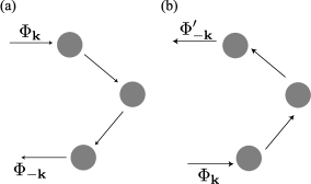
Figure 1: The finial state of the scattering path shown in (a), $\Phi_{\bf-k}$, combines with the final state of the scattering path shown in (b), $\Phi^{\prime}_{\bf-k}$, to suppress the total backscattering amplitude, $\Phi_{\bf-k}+\Phi^{\prime}_{\bf-k}$, due to the Berry’s phase. The two scattering paths, (a) $\Phi_{\bf k}\to\cdots\to\Phi_{\bf-k}$ and (b) $\Phi_{\bf k}\to\cdots\to\Phi^{\prime}_{\bf-k}$, are related with each other by “time-reversal”.

This, absence of backward scattering mechanism provides us with a simple solution explaining the high mobility, and the existence of a singularity at the Dirac point is essential to the nontrivial phase shift of $\pi$. However, it is not obvious whether the wave functions realizing in graphene nanoribbons can acquire a nontrivial Berry’s phase or not. The eigen state near the edge is the standing wave resulting from the interference between an incident wave and the edge reflected wave. If the Berry’s phase for the standing wave is trivial, then the scatters, such as a potential disorder created by charge impurities, may give rise to backward scattering. As a result, the mobility of a graphene nanoribbon decreases considerably than that of a carbon nanotube. Chen et al. (2007); Stampfer et al. (2009); Han et al. (2010); Gallagher et al. (2010) In the present paper, we study the Berry’s phases of the standing waves near the zigzag and armchair edges, and their effects on the local density of states and the transport properties of graphene nanoribbons.

In Fig. 2, we consider the zigzag edge parallel to the $x$-axis, by which translational symmetry along the $y$-axis is broken. Thus, the incident state with wave vector $(k_{x},k_{y})$ is elastically scattered by the zigzag edge, and the wave vector of the reflected state becomes $(k_{x},-k_{y})$. By contrast, the armchair edge parallel to the $y$-axis breaks translational symmetry along the $x$-axis, so that the wave vector of the reflected state is $(-k_{x},k_{y})$. Since the Brillouin zone (BZ) is given by rotating the hexagonal lattice by 90^∘, one can see in Fig. 2 that for the incident state near the K point, the reflected state by the zigzag edge is also near the K point, while the reflected state by the armchair edge is near the K^′ point. Hence, the scattering by the zigzag edge is intravalley scattering, while that by the armchair edge is intervalley scattering.

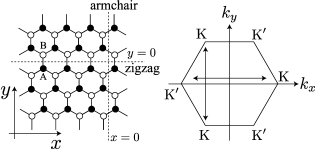
Figure 2: A hexagonal unit cell of graphene consists of A (solid circle) and B (open circle) atoms. The $xy$ coordinate system is fixed as shown. (right) The hexagon represents the first BZ of graphene, and the corners of the hexagon are K and K^′ points.

To begin with, let us consider the scattering problem for the zigzag edge. Since the zigzag edge is not the source of intervalley scattering, we focus on only the electrons near the K point. The incident and reflected waves are represented by the Bloch states. The Bloch state in the conduction energy band is written as

$$\Phi_{{\rm K},{\bf k}}^{c}({\bf r})=\frac{e^{i{\bf k}\cdot{\bf r}}}{\sqrt{V}}\phi_{{\rm K},{\bf k}}^{c},\ \ \phi_{{\rm K},{\bf k}}^{c}=\frac{1}{\sqrt{2}}\begin{pmatrix}e^{-i\theta({\bf k})}\cr 1\end{pmatrix},$$ (4)

where $V$ is the area of sample, ${\bf k}$ is the momentum measured from the K point, and $\theta({\bf k})$ is the polar angle between the vector ${\bf k}$ and the $k_{x}$-axis. Note that the Bloch function acquires a nontrivial Berry’s phase of $-\pi$ by a rotation of the wave vector around the K point as

$$\int_{0}^{2\pi}\langle\phi_{{\rm K},{\bf k}}^{c}|\frac{1}{i}\frac{\partial}{\partial\theta}|\phi_{{\rm K},{\bf k}}^{c}\rangle d\theta=-\pi.$$ (5)

The standing wave modes arise from the interference between the incident waves and the reflected waves. Let the wave vector of the incident wave be ${\bf k}=(k_{x},k_{y})$. Then the vector of the elastically reflected wave is given by ${\bf k^{\prime}}=(k_{x},-k_{y})$, and the standing wave near the zigzag edge is written as

$$\Psi_{{\rm K},{\bf k}}^{c}({\bf r})=\Phi_{{\rm K},{\bf k}}^{c}({\bf r})+e^{iz}\Phi_{{\rm K},{\bf k^{\prime}}}^{c}({\bf r}),$$ (6)

where the phase $e^{iz}$ should be determined in such a manner that $\Psi_{{\rm K},{\bf k}}^{c}({\bf r})$ [$={}^{t}(\Psi^{c}_{{\rm K},{\bf k},{\rm A}}({\bf r}),\Psi^{c}_{{\rm K},{\bf k},{\rm B}}({\bf r}))$] satisfies the boundary condition Berry et al. (1987). We take the following boundary condition for the zigzag edge Brey and Fertig (2006),

$$\lim_{y\to 0}\Psi^{c}_{{\rm K},{\bf k},{\rm B}}({\bf r})=0,$$ (7)

which describes a situation in which the B-atoms located slightly above the horizontal dashed line at $y=0$ in Fig. 2 are separated from the lower semi-infinite graphene for $y<0$. The boundary condition of Eq. (7) is satisfied when $e^{iz}=-1$, and the standing wave is written as

$$\Psi^{c}_{{\rm K},{\bf k}}({\bf r})=\frac{e^{ik_{x}x}}{\sqrt{L_{x}}}N(y)\begin{pmatrix}\sin\left(k_{y}y-\theta({\bf k})\right)\cr\sin\left(k_{y}y\right)\end{pmatrix},$$ (8)

where $L_{x}$ is the length of the zigzag edge, and $N(y)=N\neq 0$ for $y\leq 0$ and $N(y)=0$ otherwise. The value of $N$ is determined by the normalization condition. We note that the standing wave of Eq. (6) reproduces the result of tight-binding lattice model (see Appendix B of Ref.Sasaki et al., 2009).

First, we examine the Berry’s phase of the standing wave. For simplicity, let us consider the case $\theta({\bf k})=\pi/2$ for Eq. (8). This corresponds to a normal incident process to the zigzag edge [$k_{x}=0$ and $k_{y}>0$]. The amplitude for this process does not vanish as

$$\Psi^{c}_{{\rm K},k_{y}}({\bf r})=\frac{N(y)}{\sqrt{L_{x}}}\begin{pmatrix}-\cos\left(k_{y}y\right)\cr\sin\left(k_{y}y\right)\end{pmatrix}.$$ (9)

This standing wave includes a backward scattering amplitude, and the existence of the backward scattering amplitude indicates that the Berry’ phase of the standing wave vanishes. Indeed, since $\theta({\bf k}^{\prime})=-\theta({\bf k})$, the Berry’s phase of the reflected state is given by $+\pi$ as

$$\int_{0}^{2\pi}\langle\phi_{{\rm K},{\bf k^{\prime}}}^{c}|\frac{1}{i}\frac{\partial}{\partial\theta}|\phi_{{\rm K},{\bf k^{\prime}}}^{c}\rangle d\theta=+\pi,$$ (10)

while that of the incident state is $-\pi$ [see Eq. (5)]. The Berry’s phase of $-\pi$ for the incident state is canceled by the Berry’s phase of $\pi$ for the reflected state, and hence the Berry’s phase for the standing wave vanishes in total. The trivial Berry’s phase can be understood from Eq. (8), in which the Bloch function of the standing wave is real Simon (1983).

Next, we study the standing wave near the armchair edge. The K and K^′ points need to be considered simultaneously in the case of armchair edge since the armchair edge is the source of intervalley scattering. Suppose that the wave vector of the incident wave measured from the K point is ${\bf k}=(k_{x},k_{y})$. Thus, the wave vector of the elastically reflected wave measured from the K^′ point is given by ${\bf k^{\prime}}=(-k_{x},k_{y})$, and the standing wave is written as

$$\Psi^{c}_{{\bf k}}({\bf r})=\Phi^{c}_{{\rm K},{\bf k}}({\bf r})+e^{ia}\Phi^{c}_{{\rm K^{\prime}},{\bf k^{\prime}}}({\bf r}).$$ (11)

It can be shown that the Bloch state near the K^′ point is given by $\Phi^{c}_{{\rm K^{\prime}},{\bf k^{\prime}}}({\bf r})=(e^{i{\bf k^{\prime}}\cdot{\bf r}}/\sqrt{V})\phi^{c}_{{\rm K},{\bf k}}$ Sasaki et al. (2010). Thus, we may write

$$\Psi^{c}_{{\bf k}}({\bf r})=\frac{e^{ik_{y}y}}{\sqrt{L_{y}}}N(x)\phi^{c}_{{\rm K},{\bf k}}\begin{pmatrix}e^{+ik_{x}x}\cr e^{ia}e^{-ik_{x}x}\end{pmatrix},$$ (12)

where $N(x)=N\neq 0$ for $x\leq 0$ and $N(x)=0$ otherwise. The relative phase $e^{ia}$ can be determined by the boundary condition for armchair edge. The value of $e^{ia}$ must be $-i$, which will be derived elsewhere. Sasaki and Wakabayashi (2010) Note that the Bloch functions for the K and K^′ points are the same. Thus, the Berry’s phase of the standing wave near the armchair edge is given by $-\pi$. As a result, we can expect that the absence of backward scattering mechanism is valid near the armchair edge. Note, however, that the absence of backward scattering mechanism for the armchair edge is not identical to that discussed so far for carbon nanotubes. This is because the notion of a “time-reversal pair” of scattered waves in the original argument Ando et al. (1998) should be replaced to a true time-reversal pair of scattered waves near the armchair edge. The time-reversal state of Eq. (12) is given by Sasaki and Saito (2008)

$${\cal T}\Psi^{c}_{{\bf k}}({\bf r})=\frac{e^{-ik_{y}y}}{\sqrt{L_{y}}}N(x)(\phi^{c}_{{\rm K},{\bf k}})^{*}\begin{pmatrix}e^{-ia}e^{+ik_{x}x}\cr e^{-ik_{x}x}\end{pmatrix}.$$ (13)

A magnetic field breaks time-reversal symmetry, so that it invalidates the new absence of backward scattering mechanism and leads to weak anti-localization. It is also interesting to point out that the Berry’s phase for the standing wave near the armchair edge is robust against an ordinary mass term, while it is not robust against a topological mass term Haldane (1988).

The appearance of a nontrivial Berry’s phase is related to a singularity in parameter space Berry (1984); Simon (1983). Here, we show the relationship between the singularity at the Dirac point (${\bf k}=0$) in the momentum space and the standing wave. For the zigzag edge, $k_{x}$ is a continuous variable, and therefore the spectrum with $k_{y}=0$ may cross the Dirac singularity. However, Eq. (8) shows that the standing wave with $k_{y}=0$ does not exist, that is $\Psi_{{\rm K},k_{y}=0}^{c}({\bf r})=0$. Thus, the Dirac singularity seems to be separated from the spectrum of the standing wave. To explore this point further, we consider a zigzag nanoribbon by introducing another zigzag edge at $y=-L$, in addition to the zigzag edge at $y=0$. Suppose that the edge atoms at $y=-L$ are B-atoms, which imposes the boundary condition on the wave function at $y=-L$ as $\lim_{y=-L}\Psi_{{\rm K},{\bf k},{\rm A}}^{c}({\bf r})=0$. This leads to the constraint equation for $(k_{x},k_{y})$,

$$k_{y}L+\theta({\bf k})=n\pi,$$ (14)

where $n$ is an integer. We note that this equation provides the solutions of $-k_{x}=k_{y}/\tan(k_{y}L)$ which was obtained by Brey and Fertig in Ref. Brey and Fertig, 2006 [the minus sign in front of $k_{x}$ is a matter of notation]. Note that $n$ must be a nonzero integer because the equation does not possess a solution when $n=0$. In Fig. 3, we plot the solutions of Eq. (14) for the cases $n=1$ and 2. The solution for $n>2$ is given by shifting the curve for $n=2$ by $\pi/L$, and only the solution with $n=1$ shows an anomalous feature. The curve with $n=1$ approaches a point on the $k_{x}$-axis. This behavior can be checked by setting $\theta({\bf k})=\pi+k_{y}/k_{x}$ in Eq. (14) with $n=1$. It is appropriate to refer to this state with $k_{x}=-1/L$ and $k_{y}=0$ as the critical state Sasaki et al. (2005) because this state is neither the standing wave nor the edge state Fujita et al. (1996). The fact that no curve crosses the Dirac singularity is consistent to the absence of a nontrivial Berry’s phase for the standing wave. In other words, an electron can not approach the Dirac singularity due to the presence of the zigzag edge. As a result, an energy gap appears in the spectrum of the standing wave. The minimum energy gap is determined by the critical state as $E_{\rm gap}=2\hbar v_{\rm F}/L$ where $v_{\rm F}$ is the Fermi velocity. In contrast to the boundary condition for the zigzag edge, the boundary condition for the armchair edge does not forbid an electronic state cross the Dirac singularity point, and therefore the electron can pick up a nontrivial Berry’s phase.

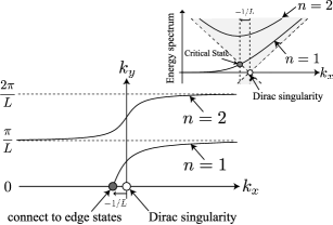
Figure 3: The curves represent the solutions of parameters $k_{x}$ and $k_{y}$ which are allowed by the boundary condition for a zigzag nanoribbon. The Dirac singularity is not located on the curves, which shows that there is no singularity at the parameter space of the standing waves. The inset shows the corresponding spectral flow in the energy dispersion relation.

Here, we consider pseudospin of the standing wave in order to examine the local density of states (LDOS) near the zigzag edge. The pseudospin for an eigenstate $\Psi(y)$ is defined by the expectation value of Pauli matrices as $\langle\sigma_{i}\rangle\equiv\int\sigma_{i}(y)dy$ ($i=x,y,z$) where $\sigma_{i}(y)$ is a pseudospin density defined by $\sigma_{i}(y)\equiv\Psi^{\dagger}(y)\sigma_{i}\Psi(y)$. The boundary condition of Eq. (7) means that the pseudospin density is polarized into the positive $z$-axis locally near the zigzag edge, that is, $\sigma_{z}(0)>0$ and $\sigma_{x}(0)=\sigma_{y}(0)=0$. Actually, by putting $y\simeq 0$ into Eq. (8), we see that the standing wave near the zigzag edge has amplitudes only on A-atoms. This polarization of the pseudospin causes an anomalous behavior to appear in the LDOS near the zigzag edge. To show this, let us first review the LDOS for a graphene without an edge. Assuming that electrons are non-interacting, the bulk LDOS is given by

$$\rho(E)=\frac{1}{2\pi}\frac{|E|}{(\hbar v_{\rm F})^{2}},$$ (15)

where $\rho(E)$ is proportional to $|E|$, which results from the Dirac cone spectrum. The LDOS near the zigzag edge can be calculated by using the standing wave given in Eq. (8). The LDOS has the form,

$$\rho_{s}(E,y)=\frac{1}{2\pi}\frac{|E|}{(\hbar v_{\rm F})^{2}}R(E,y),$$ (16)

where $R(E,y)$ is defined as

$$R(E,y)\equiv\frac{1}{\pi}\int^{\pi}_{0}d\theta\Psi_{{\rm K},{\bf k}}(y)^{\dagger}\Psi_{{\rm K},{\bf k}}(y).$$ (17)

By performing the integral with respect to the angle $\theta$ in Eq. (17), we obtain the analytical result for $R(E,y)$ as

$$R(E,y)=1-\frac{1}{2}\left\{J_{0}\left(2\frac{|Ey|}{\hbar v_{\rm F}}\right)+J_{2}\left(2\frac{|Ey|}{\hbar v_{\rm F}}\right)\right\},$$ (18)

where $J_{\nu}(x)$ is a Bessel function of order $\nu$. The LDOS is symmetric with respect to $E=0$. The bulk LDOS in Eq. (15) can be reproduced by setting $|y|\to\infty$ in Eq. (18) since $J_{\nu}(\infty)=0$. In Fig. 4, we plot the LDOS at $|y|=0$, 1, 2, 3, and 6[nm]. The slope of the LDOS depends on the distance from the zigzag edge. At the edge, that is, at $|y|=0$, since $J_{0}(0)=1$ and $J_{2}(0)=0$, we see that $R(E,0)=1/2$, and the slope of $\rho_{s}(E,0)$ is half of that of $\rho_{s}(E,\infty)$ [$=\rho(E)$]. This results from the fact that the amplitudes at one of two sublattice disappears near the zigzag edge (due to the pseudospin polarization), and only the half of the amplitude in the unit cell can contribute to the LDOS.

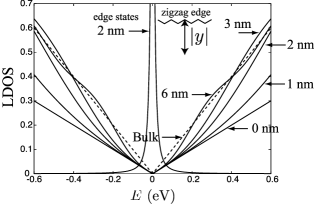
Figure 4: The position dependence of the LDOS structure near the zigzag edge. The peak structure at $E=0$ is due to the edge states.

In Fig. 4, in addition to the LDOS due to the standing wave, we plot the LDOS (at $|y|=2$[nm]) due to the edge states Fujita et al. (1996); Nakada et al. (1996). The edge states produce a peak at $E=0$ in the LDOS. The LDOS of the edge states is calculated as follows. The wave function of the edge state is given by Sasaki and Wakabayashi (2010)

$$\Psi_{{\rm K},k_{x}}({\bf r})=\frac{e^{ik_{x}x}}{\sqrt{L_{x}}}N(y)\sqrt{2|k_{x}|}e^{k_{x}|y|}\begin{pmatrix}1\cr 0\end{pmatrix}.$$ (19)

Note that the edge states appear for $k_{x}<0$ and $y<0$ (see Fig. 3). Since the energy eigenvalue of the edge state vanishes, the LDOS for the edge states is written as

$$\rho_{e}(E,y)=\frac{\delta}{\pi}\sum_{k_{x}<0}\frac{\Psi_{{\rm K},k_{x}}({\bf r})^{\dagger}\Psi_{{\rm K},k_{x}}({\bf r})}{(E-0)^{2}+\delta^{2}},$$ (20)

where $\delta$ is a phenomenological parameter representing energy uncertainty of the edge states, for which we assume $\delta=10$ meV. Substituting $\sum_{k_{x}<0}$ with $(L_{x}/2\pi)\int_{-\infty}^{0}dk_{x}$ in Eq. (20), and performing the integral for $k_{x}$, we obtain

$$\rho_{e}(E,y)=\frac{1}{2\pi^{2}}\frac{2\delta}{E^{2}+\delta^{2}}\frac{1}{4y^{2}}.$$ (21)

This result has been used in Fig. 4 to plot the LDOS of the edge states. Note that $\rho_{e}(E,y)$ decreases as $\sim y^{-2}$, which is a slowly decreasing function compared with the exponential decaying wave function of the edge state. It is interesting to note that $\rho_{e}(E,y)\sim y^{-2}$ can be derived from the fact that $\int_{0}^{E_{c}}\{\rho_{s}(E,y)+\rho_{e}(E,y)\}dE$ does not depend on $y$ for a large value of $E_{c}$. This is a sum rule for the total LDOS consisting of the edge states and the standing waves, in which the density above (below) the Fermi energy at $E=0$ must be position independent. This argument also shows that the singular behavior of the LDOS for the edge states at $y=0$ is a consequence of the wave function of the standing wave.

By examining the standing wave near the graphene edge, we have seen that the armchair edge preserves a non-trivial Berry’s phase as in the bulk of graphene, on the other hand, such a non-trivial phase is absent for the standing wave near the zigzag edge. Here, we consider the indication of this result with respect to the transport in graphene nanoribbons. In the argument for the absence of the backward scattering given in the introduction (see Fig. 1), we find, by replacing $\Phi_{\bf k}$ with the standing wave $\Psi_{\bf k}$, that the backscattering amplitude, $\Psi_{\rm bs}=\left[1+U(2\pi)\right]\Psi_{\bf-k}$, is enhanced for zigzag nanoribbons (due to $U(2\pi)=1$), while it still vanishes for armchair nanoribbons (due to $U(2\pi)=-1$). Thus, we can expect that the conductance of a zigzag nanoribbon is smaller than that of an armchair nanoribbon, if we assume only scatters with long-range potential. The simulations performed by Areshkin et al. Areshkin et al. (2007) and Yamamoto et al. Yamamoto et al. (2009) show indeed that long-range potentials are ineffective in causing backscattering in a perfect armchair nanoribbon. For narrow metallic armchair nanoribbons, the linear energy dispersion originating from the Dirac point provides a nearly perfect conduction, and this nearly perfect conduction might relate to the nontrivial Berry’s phase since the linear energy dispersion picks up the Dirac singularity. Note, however, that the standing wave for the armchair edge is a short-length intervalley mode, that is, the electronic wave length of the standing wave is order of the lattice constant. As a result, the wave function can be very sensitive to a short-range scattering potential, such as irregular edges Areshkin et al. (2007) and lattice vacancies Li and Lu (2008). An armchair nanoribbon has both advantages (non-trivial Berry’s phase) and disadvantages (intervalley mode) for the transport as well as that a zigzag nanoribbon has both advantages (intravalley mode) and disadvantages (trivial Berry’s phase). Therefore, in a realistic situation, it is reasonable to consider that a nanoribbon does not exhibit an electronic conduction comparable to a metallic carbon nanotube.

It seems that recent tight-binding numerical studies show that the conductance of zigzag nanoribbons is more robust than that of armchair nanoribbons against edge disorders. Areshkin et al. (2007); Li and Lu (2008); Cresti and Roche (2009a, b) In the numerical studies, the transport given by the electrons which are located very close to the Fermi level is concerned. For zigzag nanoribbons, the propagating modes in each valley contain a single one-way excess channel (the states on the curve of $n=1$ which are close to the critical state shown in Fig. 3). This feature causes a perfectly conducting channel to appear in the disordered system for the case that impurities do not give rise to intervalley scattering Wakabayashi et al. (2007, 2009). This feature also seems to cause a robust conducting channel to appear in the edge disordered system. Areshkin et al. (2007); Li and Lu (2008); Cresti and Roche (2009a, b) For our discussion of the backscattering in zigzag nanoribbons, we assume that the initial state with momentum $k_{x}$ accompanies the corresponding final state with $-k_{x}$. This condition is not satisfied for the single one-way excess channel, for which our discussion for the Berry’s phase is useless. The single one-way excess channel plays a dominant role in zigzag nanoribbons of the widths up to several nanometers for a limited energy window. Areshkin et al. (2007) Our result for the Berry’s phase may be useful in discussing transport of zigzag nanoribbons of the widths more than 10 nm, for which we have several number of channels having the final state with $-k_{x}$.

Our result may have a relationship to the formation of a transport gap observed for graphene nanoribbons. Stampfer et al. (2009); Han et al. (2010); Gallagher et al. (2010) Note that the standing wave near a realistic rough edge can be described as the sum of the standing waves for zigzag and armchair edges. Sasaki et al. (2010) Since the standing wave for zigzag edge is a long-length intravalley mode and that for armchair edge is a short-length intervalley one, their characters do not interfere with each other and can coexist in the standing wave near a rough edge. This is also indicative of that a small portion of zigzag edge in a rough edge eventually governs the long-length transport behavior of a nanoribbon, as is numerically simulated by several authors. Evaldsson et al. (2008); Mucciolo et al. (2009) Indeed, Gallagher et al. Gallagher et al. (2010) and Han et al. Han et al. (2010) observed that the source-drain gap has a strong dependence on ribbon’s length. It is also important to recognize that there are two distinct localized states; the edge states and localized states which consist of the standing waves. Since the localization length of the former is on the order of lattice constant, it is difficult to consider that the transport behavior of nanoribbons of the widths larger than $10$ nm is dominated by the edge states. Martin and Blanter (2009) In contrast, the latter is caused by the scatters, such as a potential disorder created by charge impurities, giving rise to backward scattering. Since the latter consists of the standing waves, there is a possibility that the localization length is the order of the width of a ribbon. Han et al. Han et al. (2010) measured electron transport in lithographically fabricated nanoribbons of widths $20<W<120$ nm with rough edge on the order of nanometers, and confirmed that the size of a transport gap is inversely proportional to the ribbon width.

In conclusion, we have shown that the Berry’s phase for the standing wave near the zigzag edge is trivial. The momentum parameter space for the standing wave near the zigzag edge does not include the Dirac singularity, which is essential to the absence of a non-trivial Berry’s phase. As a result, the absence of backward scattering mechanism that works well in a metallic carbon nanotube can not be used for a zigzag nanoribbon. The absence of the Dirac singularity in the momentum space of the standing wave results in the peak in the LDOS due to the edge states. An observation of the LDOS peak near the zigzag edge is a direct evidence of the absence of the Dirac singularity in the parameter space of the standing wave. In contrast, a non-trivial Berry’s phase survives the reflection by the armchair edge. For the standing wave near the armchair edge, we obtain the new absence of backward scattering mechanism in which a real time-reversal pair of backward scattered waves cancels with each other. This absence of the backward scattering mechanism for the armchair edge is not robust against a short-range scattering potential since the standing wave is a short-length intervalley mode. An armchair nanoribbon has both advantage and disadvantage for the transport as well as a zigzag nanoribbon.

References

- Chen et al. (2007) Z. Chen, Y.-M. Lin, M. J. Rooks, and P. Avouris, Physica E 40, 228 (2007).
- Stampfer et al. (2009) C. Stampfer, J. Güttinger, S. Hellmüller, F. Molitor, K. Ensslin, and T. Ihn, Phys. Rev. Lett. 102, 056403 (2009).
- Han et al. (2010) M. Y. Han, J. C. Brant, and P. Kim, Phys. Rev. Lett. 104, 056801 (2010).
- Gallagher et al. (2010) P. Gallagher, K. Todd, and D. Goldhaber-Gordon, Phys. Rev. B 81, 115409 (2010).
- Berry (1984) M. V. Berry, Proc. R. Soc. London A 392, 45 (1984).
- Simon (1983) B. Simon, Phys. Rev. Lett. 51, 2167 (1983).
- Ando et al. (1998) T. Ando, T. Nakanishi, and R. Saito, J. Phys. Soc. Jpn. 67, 2857 (1998).
- Berry et al. (1987) M. V. Berry, F. R. S, and R. J. Mondragon, Proc. R. Soc. Lond. A 412, 53 (1987).
- Brey and Fertig (2006) L. Brey and H. A. Fertig, Phys. Rev. B 73, 235411 (2006).
- Sasaki et al. (2009) K. Sasaki, M. Yamamoto, S. Murakami, R. Saito, M. Dresselhaus, K. Takai, T. Mori, T. Enoki, and K. Wakabayashi, Phys. Rev. B 80, 155450 (2009).
- Sasaki et al. (2010) K. Sasaki, R. Saito, K. Wakabayashi, and T. Enoki, J. Phys. Soc. Jpn. 79, 044603 (2010).
- Sasaki and Wakabayashi (2010) K. Sasaki and K. Wakabayashi, arXiv:1003.5036 (2010).
- Sasaki and Saito (2008) K. Sasaki and R. Saito, Prog. Theor. Phys. Suppl. 176, 253 (2008).
- Haldane (1988) F. D. M. Haldane, Phys. Rev. Lett. 61, 2015 (1988).
- Sasaki et al. (2005) K. Sasaki, S. Murakami, R. Saito, and Y. Kawazoe, Phys. Rev. B 71, 195401 (2005).
- Fujita et al. (1996) M. Fujita, K. Wakabayashi, K. Nakada, and K. Kusakabe, J. Phys. Soc. Jpn. 65, 1920 (1996).
- Nakada et al. (1996) K. Nakada, M. Fujita, G. Dresselhaus, and M. S. Dresselhaus, Phys. Rev. B 54, 17954 (1996).
- Areshkin et al. (2007) D. A. Areshkin, D. Gunlycke, and C. T. White, Nano Letters 7, 204 (2007).
- Yamamoto et al. (2009) M. Yamamoto, Y. Takane, and K. Wakabayashi, Phys. Rev. B 79, 125421 (2009).
- Li and Lu (2008) T. C. Li and S.-P. Lu, Phys. Rev. B 77, 085408 (2008).
- Cresti and Roche (2009a) A. Cresti and S. Roche, New Journal of Physics 11, 095004 (2009a).
- Cresti and Roche (2009b) A. Cresti and S. Roche, Phys. Rev. B 79, 233404 (2009b).
- Wakabayashi et al. (2007) K. Wakabayashi, Y. Takane, and M. Sigrist, Phys. Rev. Lett. 99, 036601 (2007).
- Wakabayashi et al. (2009) K. Wakabayashi, Y. Takane, M. Yamamoto, and M. Sigrist, New Journal of Physics 11, 095016 (2009).
- Evaldsson et al. (2008) M. Evaldsson, I. V. Zozoulenko, H. Xu, and T. Heinzel, Phys. Rev. B 78, 161407 (2008).
- Mucciolo et al. (2009) E. R. Mucciolo, A. H. Castro Neto, and C. H. Lewenkopf, Phys. Rev. B 79, 075407 (2009).
- Martin and Blanter (2009) I. Martin and Y. M. Blanter, Phys. Rev. B 79, 235132 (2009).