Typhoon eye trajectory based on a mathematical model: comparing with observational data

Abstract

We propose a model based on the primitive system of the Navier-Stokes equations in a bidimensional framework as the $l$ - plane approximation, which allows us to explain the variety of tracks of tropical cyclones (typhoons). Our idea is to construct special analytical solutions with a linear velocity profile for the Navier-Stokes systems. The evidence of the structure of linear velocity near the center of vortex can be proven by the observational data. We study solutions with the linear-velocity property for both barotropic and baroclinic cases and show that they follow the same equations in describing the trajectories of the typhoon eye at the equilibrium state (that relates to the conservative phase of the typhoon dynamics). Moreover, at the equilibrium state, the trajectories can be viewed as a superposition of two circular motions: one has period $2\pi/l,$ the other one has period $2\pi/b_{0},$ where $l$ is the Coriolis parameter and $b_{0}$ is the height-averaged vorticity at the center of cyclone.

Also, we compare our theoretical trajectories based on initial conditions from the flow with tracks obtained from the observational database. It is worth to mention that under certain conditions our results are still compatible with observational data although we did not truly consider the influence of steering effect. Finally, we propose the parameter-adopting method so that one could correct the weather prediction in real time. Examples of our analysis and the use of parameter-adopting method for the historic trajectories are provided.

1 Introduction

Tropical cyclones, commonly known as hurricanes in the North Atlantic Ocean and typhoons in the western North Pacific Ocean, are one of the most devastating weather phenomena in the world. The intense winds associated with tropical cyclone often generate ocean waves and heavy rain, which usually result in severe disasters. To reduce the harm caused by the tropical cyclones, the most important issue is the prediction of its moving trajectory.

For a long time, the phenomenon of formation of a huge intense atmospheric vortex attracted attentions of scientists working in various fields (e.g. see [1] and references in [2]). A large progress has been made in the last decade in understanding the physical process and the quality of operational prediction of tropical cyclones ([3],[4], and references therein). In particular, statistical and numerical weather prediction models have been improved dramatically and used to provide operational forecasters the high-quality prediction for national weather bureaus.

The system of equations served for the numerical prediction is very complicated. It needs to take many factors into account, for examples, phase transitions, vertical advection, and boundary layer effects, etc. Generally, it is difficult to use such system to comprehend its underlying physical processes. To have a conceptual understanding about these processes, some assumptions must be made to simplify the equations. The solutions then may appear in a simpler form so that it becomes much easier to gain their physical interpretations. However, neglecting some terms in the equations may risk losing some important properties of the system, e.g. the symmetries. Therefore, it is very important to find particular solutions for the untruncated system of equations and to adjust them to track some particular phenomena. In the present paper, we seek special solutions for the primitive air-motion system. As we should show later, these solutions can be considered as a model of the typhoon when it is near its center.

Our model is bidimensional and we does not consider the effect of heating that results from a coupling between the latent heat released in the clouds and the vertical wind shear. It is known that a great variety of the vortex phenomenon can be explained in the frame of two-dimensional models if we consider the vertical dimension as a small scale comparing with the horizontal ones (e.g. [5]). In meteorology, this concept is often adopted in studying the processes for middle and large scales [6]. In this case, the atmosphere is regarded to be ”thin”. For example, the meteorologists often consider the atmosphere as a one-layer fluid in the barotropic framework without specifying the vertical coordinate. This bidimensional theory, despite such simplicity, can use to explain many observed features of the tropical cyclone motions [3]. However, the essence of bidimensionality in our model differs from above. We derived it from a primitive complete three-dimensional system of equations by averaging the system over the height, so the vertical processes of the system are presented in a hidden form.

The paper is organized as follows. In section 2, we study the derivation of a bidimensional model of the atmosphere dynamics based on the primitive Navier-Stokes equations for compressible viscous heat-conductive gas in the physical 3D space. In section 3, we investigate polynomial solutions for both barotropic and baroclinic system and find that the equations which govern the trajectories at the equilibrium point are the same in both cases. In section 4, we test possible trajectories of the typhoon center with various input parameters and demonstrate that our the artificial trajectories can imitate the behavior of the typhoon eye tracks. Moreover, numerical simulation shows that the motion of the vortex center provided by our explicit algebraic formulas is reasonably close to the motion of a developed vortex when it is near the equilibrium. In section 5, we examine two different types of historical typhoons: Man Yi (parabolic trajectory) and Parma (loop), with our theoretical results. Here, we propose a method of the parameter-fitting that allows us to predict the trajectory of typhoon eye only based on three successive points in the past. In section 6, we further investigate the situation when the typhoon encounters the shore. In this case, the typhoon may disappear due to the destruction of the stable vortex. Finally, discussions about our topics and future work are provided in section 7.

2 Bidimensional models of the atmosphere dynamics

The motion of compressible rotating, viscous, heat-conductive, Newtonian polytropic gas in ${\mathbb{R}}\times{\mathbb{R}}^{3},$ is governed by the compressible Navier-Stokes equations [7]

$$\partial_{t}\rho+{\rm div}(\rho u)=0,$$

$$\partial_{t}(\rho u)+{\rm Div}(\rho u\otimes u)+\nabla p+2\omega\times u={\rm Div}T,$$

$$\partial_{t}\left(\frac{1}{2}\rho|u|^{2}+\rho e\right)+{\rm div}\left((\frac{1}{2}\rho|u|^{2}+\rho e+p)u\right)={\rm div}(Tu)+\nabla(\kappa,\nabla\theta),$$

where $\rho,\,u=(u_{1},u_{2},u_{3}),\,p,\,e,\,\theta\,$ denote the density, velocity, pressure, internal energy and absolute temperature, respectively. Here $\omega=(\omega_{1},\omega_{2},\omega_{3})$ is the angular velocity of the Earth rotation, $\kappa=(\kappa_{1},\kappa_{2},\kappa_{3})^{T},\,\kappa_{i}\geq 0,\,i=1,2,3,$ is the vector of heat conduction. The stress tensor $\,T\,$ is given by the Newton law

$$T=T_{ij}=\mu\,(\partial_{i}u_{j}+\partial_{j}u_{i})+\lambda\,{\rm div}u\,\delta_{ij},$$

where the constants $\mu$ and $\lambda$ are the coefficient of viscosity, and the second coefficient of viscosity. Here ${\rm Div}$ and $\rm div$ stand for the divergency of tensor and vector, respectively, $\otimes$ denotes the tensor product of vectors.

The state equations are

$$p=R\rho\theta,\quad e=c\theta,\quad p=A\exp\left(\frac{s}{c}\right)\rho^{\tilde{\gamma}}.$$

Here $A>0$ is a constant, $R$ is the universal gas constant, $s=\log e-(\gamma-1)\log\rho$ is the specific entropy, $c=\frac{R}{\tilde{\gamma}-1},$ $\tilde{\gamma}>1$ is the specific heat ratio.

The state equations (2.5) imply

$$\,p=(\tilde{\gamma}-1)\rho e,$$

which allows us to consider (2.1) – (2.3) as a system of equations for the unknowns $\rho,\,u,\,p.$ Indeed, from (2.1) – (2.3) and (2.6), we arrive

$$\partial_{t}p+(u,\nabla p)+\tilde{\gamma}p\,{\rm div}u=(\tilde{\gamma}-1)\,\sum\limits_{i,j=1}^{n}\,T_{ij}\partial_{j}u_{i}+\frac{\kappa}{R}\,\Delta\frac{p}{\rho}.$$

For simplicity, we denote the system (2.1), (2.2), (2.7) as (NS).

Let ${\bf x}=(x_{1},x_{2})$ be a point on the Earth surface, $\varphi_{0}$ be the latitude of some fixed point ${\bf x}_{0}.$ Following from [8] (early this approach was used in [9] for barotropic atmosphere), we derive a spatially two-dimensional system for (NS). Let us introduce $\hat{\phi}$ and $\bar{f}$ to represent for taking the average of $\phi$ and $f$ over the height respectively, namely, $\displaystyle\hat{\phi}:=\int_{0}^{\infty}\phi\,dz,\quad\bar{f}:=\frac{1}{\hat{\rho}}\int_{0}^{\infty}\rho f\,dz.$ where $\phi$ and $f$ are arbitrary functions, and denote $\varrho(t,{\bf x})=\hat{\rho},\,P(t,{\bf x})=\hat{p},\,{\bf U}(t,{\bf x})=\bar{u},\,{\Theta}(t,{\bf x})=\bar{\theta}.$ Moreover, the usual adiabatic exponent, $\tilde{\gamma}$ is related to the “two-dimensional” adiabatic exponent $\gamma$ as follows: $\gamma=\displaystyle\frac{2\tilde{\gamma}-1}{\tilde{\gamma}}<\tilde{\gamma}.$

Now, we include the impenetrability conditions in our model. These conditions ensure that the derivatives of the velocity equal to zero on the Earth surface and a sufficiently rapid decay for all thermodynamic quantities as the vertical coordinate $z$ approaches to infinity. In other words, the impenetrability conditions make sure the boundedness of the mass, energy, and momentum in the air column. They also provide the necessary conditions for the convergence of integrals .

Let us denote additionally $l=2\omega_{3}\sin\varphi_{0}$ (the Coriolis parameter) and $\quad L=\left(\begin{array}[]{cr}0&-1\\ 1&0\end{array}\right).$

In this way, one can get the system as the $l$- plane approximation near ${\bf x}_{0}$:

$$\varrho(\partial_{t}{\bf U}+({\bf U}\cdot\nabla){\bf U}+lL{\bf U}+\nabla P)=T_{1}(\bf U),$$

$$\partial_{t}\varrho+\nabla\cdot(\varrho{\bf U})=0,$$

$$\partial_{t}P+({\bf U},\nabla P)+\gamma P\,{\rm div}{\bf U}=(\gamma-1)\,T_{2}({\bf U})+\kappa(\frac{1}{R}\,\Delta\Theta-\xi),$$

where

$$T_{1}({\bf U})={\rm Div}{\bf T}_{ij},\quad{\bf T}_{ij}=\mu\,(\partial_{i}{\bf U}_{j}+\partial_{j}{\bf U}_{i})+\lambda\,{\rm div}{\bf U}\,\delta_{ij},$$

$$T_{2}({\bf U})=((2\mu+\lambda)((\partial_{1}{\bf U}_{1})^{2}+(\partial_{2}{\bf U}_{2})^{2})+\mu(\partial_{1}{\bf U}_{2}+\partial_{2}{\bf U}_{1})^{2}),$$

$\mu$ and $\lambda$ are the coefficients of viscosity interpreted as the coefficients of turbulent viscosity (may be not only constants). Their values are much greater than those for the molecular analogues. For simplicity, the coefficients of the heat conductivity are assumed to be constants and equal. $\xi$ is the heat flow from the ocean surface, it is also assumed to be a constant.

3 Models of the typhoon dynamics with the linear velocity profile

Suppose that the velocity vector near the origin has the form

$${\bf u}(t,{\bf x})=a(t){\bf r}+b(t){\bf r}_{\bot},$$ (3.1)

where

$${\bf r}=(x_{1},x_{2})^{T},\,{\bf r}_{\bot}=(x_{2},-x_{1})^{T}.$$

This assumption is made according to the observational data [16](see Fig.1). Moreover, as it is shown in [12], in the stable vortex, the velocity field necessarily satisfies the Cauchy-Riemann conditions, namely,

$$\frac{\partial u_{1}}{\partial x_{1}}=\frac{\partial u_{2}}{\partial x_{2}},\qquad\frac{\partial u_{1}}{\partial x_{2}}=-\frac{\partial u_{2}}{\partial x_{1}}.$$

This property holds for (3.1) and also verifies our choice for the velocity field.

Figure 1: The tangential component of (relative) velocity in $m\cdot s^{-1}$ on different stage of the typhoon formation (August 30, August 31, September 2). The hurricane Anita, North Atlantic, 1977 [16]

Note that if we do not take into account the turbulent viscosity ($\mu=\lambda=0$) and the heat transfer ($\kappa=0$) in our model. We get the system similar to the gas dynamics instead of (2.1)- (2.3). Solutions to such system were constructed and also studied in [13],[14],[15].

We next consider two forms of the system $(2.8),$ which have exact polynomial solutions.

3.1 System with respect to the velocity, pressure and entropy, without viscosity and heat conductivity

We assume $\mu=\lambda=\kappa=0$ and introduce a new variable $\pi=p^{\frac{\gamma-1}{\gamma}}.$ We also consider the 2D entropy $S$ connecting with $\varrho$ and $P$ through the state equation (2.5), where we use $\gamma$ instead of $\tilde{\gamma}.$ For the new unknown variables $\pi,{\bf U},S,$ we arrive the system [2]

$$\partial_{t}{\bf U}+({\bf U}\cdot\nabla){\bf U}+lL{\bf U}+\frac{\gamma}{\gamma-1}\exp{\frac{S}{\gamma}}\nabla\pi=\varrho^{-1}T_{1}({\bf U}),$$

$$\partial_{t}\pi+(\nabla\pi\cdot{\bf U})+(\gamma-1)\pi\,{\rm div}{\bf U}=0,$$

$$\frac{p}{R}\left(\partial_{t}S+({\bf U},\nabla S)\right)=T_{2}({\bf U}).$$

Following [10, 11], we change the coordinate system so that the origin of the new system is located at the center of the typhoon eye. Now ${\bf U}={\bf u}+{\bf V},$ where ${\bf V}(t)=(V_{1}(t),V_{2}(t))$ is the velocity of the typhoon eye propagation. Thus, we obtain a new system

$$\partial_{t}{\bf u}+({\bf u}\cdot\nabla){\bf u}+\dot{\bf V}+lL({\bf u}+{\bf V})+\frac{\gamma}{\gamma-1}\exp{\frac{S}{\gamma}}\nabla\pi=\varrho^{-1}T_{2}({\bf u}),$$ (3.2)

$$\partial_{t}\pi+\nabla\pi\cdot{\bf u}+(\gamma-1)\pi{\rm div}{\bf u}=0,$$ (3.3)

$$\frac{p}{R}\left(\partial_{t}S+({\bf u},\nabla S)\right)=T_{2}({\bf u}).$$ (3.4)

Note that in [10, 11], shallow water equations were considered. It is a particular case of (2.8) with $\gamma=2,\,S\equiv const.,\lambda=\mu=\kappa=0.$

Given the vector ${\bf V}$, the trajectory can be found by integrating the system

$$\dot{x}_{1}(t)=V_{1}(t),\qquad\dot{x}_{2}(t)=V_{2}(t).$$ (3.5)

We assume the velocity has a linear profile (3.1) and look for other components of the solution to the system (3.2)–(3.4) in the following form

$$\pi(t,{\bf x})=A(t)x_{1}^{2}+B(t)x_{1}x_{2}+C(t)x_{2}^{2}+M(t)x_{1}+N(t)x_{2}+K(t),$$ (3.6)

$$S(t,{\bf x})=S_{0}(t)+\gamma\,\ln\sum\limits_{i_{1},i_{2}=1}^{\infty}\,S_{i_{1}i_{2}}(t)x_{1}^{i_{1}}x_{2}^{i_{2}}.$$ (3.7)

Here, $T_{1}({\bf u})=T_{2}({\bf u})=0.$ Recall that $K(t)$ is the value of “renormalized” pressure $\pi$ at the center of vortex, therefore, in the physical sense, $K(t)>0.$ Substituting (3.1)–(3.7) into (3.2)–(3.4) and match the coefficients for similar term, we obtain $S_{i_{1}i_{2}}(t)\equiv 0,$ $\,i_{1},i_{2}\in\mathbb{N},\,S_{0}(t)=const,\,A(t)=C(t),$ and $\,B(t)\equiv 0.$ At the center of typhoon, there exists a domain of lower pressure. Therefore, it is natural to set $A(t)>0.$

Note that the motion near the typhoon center is “barotropic” in our solution, i.e., the pressure only depends on its density. However, this barotropicity is only for the bidimensional density and pressure. This assumption may not hold for three-dimensional cases.

Let us introduce a constant $c_{0}:=\frac{\gamma}{\gamma-1}\exp{\frac{S_{0}}{\gamma}}.$

Thus, the functions $a(t),b(t),A(t),M(t),N(t),K(t),V_{1}(t),V_{2}(t)$ satisfy the following system of ODEs:

$$\dot{A}+2\gamma aA=0,$$ (3.8)

$$\dot{a}+a^{2}-b^{2}+lb+2c_{0}A=0,$$ (3.9)

$$\dot{b}+2ab-la=0,$$ (3.10)

$$\dot{K}+2(\gamma-1)aK=0,$$ (3.11)

$$\dot{M}+(2\gamma-1)aM-bN=0,$$ (3.12)

$$\dot{N}+(2\gamma-1)aN+bM=0,$$ (3.13)

$$\dot{V}_{1}-lV_{2}+c_{0}M=0,$$ (3.14)

$$\dot{V}_{2}+lV_{1}+c_{0}N=0.$$ (3.15)

From (3.8) and (3.10), we have

$$b=\frac{l}{2}+C_{1}|A|^{1/\gamma},$$ (3.16)

where $C_{1}.$ a constant. Therefore, system (3.8) – (3.10) can be reduced to equations

$$\dot{A}=-2\gamma aA,\qquad\dot{a}=-a^{2}-\frac{l^{2}}{4}+C_{1}^{2}A^{2/\gamma}-2c_{0}A.$$ (3.17)

Further, if $A(t)$ and $a(t)$ are known, we can find other components of solutions. Namely, from (3.12) and (3.13), c we can get

$$M(t)=(M^{2}(0)+N^{2}(0))^{1/2}\exp\left(-\frac{2\gamma-1}{2}\int\limits_{0}^{t}a(\tau)d\tau\right)\sin(\frac{l}{2}t+C_{1}\int_{0}^{t}A^{1/\gamma}(\tau)d\tau+C_{2}),$$

$$N(t)=(M^{2}(0)+N^{2}(0))^{1/2}\exp\left(-\frac{2\gamma-1}{2}\int\limits_{0}^{t}a(\tau)d\tau\right)\cos(\frac{l}{2}t+C_{1}\int_{0}^{t}A^{1/\gamma}(\tau)d\tau+C_{2}).$$

From (3.8) and (3.11), we obtain

$$K(t)=C_{3}(|A(t)|)^{\frac{\gamma-1}{\gamma}}.$$

Here $C_{2},C_{3}$ are constants depending only on initial data. However, from (3.14), (3.15), and (3.5), the trajectory does not depend on $K(t).$

The phase curves of (3.17) can be found explicitly. They satisfy the algebraic equation

$$a^{2}=C_{4}A^{\frac{1}{\gamma}}-C_{1}^{2}A^{\frac{2}{\gamma}}+\frac{l^{2}}{4(\gamma-1)}+\frac{2c_{0}}{\gamma-1}A,$$ (3.18)

with the constant $C_{4}$ depending only on initial data. Our analysis shows that there exists a unique equilibrium point on the phase plane $(A,a),\,A>0$ for $1<\gamma<2$. It is a center on the axis $a=0.$ We denote this stable equilibrium as $(A_{0},0),$ where $A_{0}$ is a positive root of the equation $-\frac{l^{2}}{4}+C_{1}^{2}A^{2/\gamma}-2c_{0}A=0.$

3.2 System with respect to the velocity, density and temperature

We take the average of the first state equations (2.5) over the height to get $P=R\varrho\Theta$ and then exclude the pressure from system (2.8), we arrive

$$\varrho(\partial_{t}{\bf U}+({\bf U}\cdot\nabla){\bf U}+lL{\bf U})+R(\varrho\nabla\theta+\theta\nabla\varrho)=T_{1}({\bf U}),$$

$$\partial_{t}\varrho+(\nabla\varrho\cdot{\bf U})+\varrho\nabla{\bf U}=0,$$

$$\partial_{t}\Theta+(\nabla\Theta\cdot{\bf U})+(\gamma-1)\,\Theta\,{\rm div}{\bf U}=\frac{\gamma-1}{R}T_{2}({\bf U})+\frac{\kappa}{R\varrho}(\Delta\theta-\xi).$$

After changing the coordinates system, it takes the form

$$\varrho(\partial_{t}{\bf u}+({\bf u}\cdot\nabla){\bf u}+\dot{\bf V}+lT({\bf u}+{\bf V}))+R(\varrho\nabla\theta+\theta\nabla\varrho)=T_{1}({\bf u}),$$ (3.19)

$$\partial_{t}\varrho+(\nabla\varrho\cdot{\bf u})+\varrho\,{\rm div}{\bf u}=0,$$ (3.20)

$$\partial_{t}\Theta+(\nabla\Theta\cdot{\bf u})+(\gamma-1)\,\Theta\,{\rm div}{\bf u}\,=\,\frac{\gamma-1}{R}T_{2}({\bf u})+\frac{\kappa}{R\varrho}(\Delta\theta-\xi).$$ (3.21)

The position of the vortex center can be obtained again from (3.5).

Note that now the viscosity and heat conductivity are not neglected.

We can obtain a closed system of ordinary differential equations if we seek the solution to (3.19)–(3.21) in the following form:

$$\theta(t,{\bf x})=A_{1}(t)x_{1}^{2}+B_{1}(t)x_{1}x_{2}+C_{1}(t)x_{2}^{2}+M_{1}(t)x_{1}+N_{1}(t)x_{2}+K_{1}(t),$$ (3.22)

$$\varrho(t,{\bf x})=K_{2}(t).$$ (3.23)

Substituting (3.1), (3.22), (3.23) into (3.19)–(3.21), we obtain $A_{1}(t)=C_{1}(t),$ $B_{1}(t)=0$ and

$$\dot{A}_{1}+2\gamma aA_{1}=0,$$ (3.24)

$$\dot{a}+a^{2}-b^{2}+lb+4RA_{1}=0,$$ (3.25)

$$\dot{b}+2ab-la=0,$$ (3.26)

$$\dot{K}_{2}+2aK_{2}=0,$$ (3.27)

$$\dot{K}_{1}+2(\gamma-1)aK_{1}\,=\,\frac{2(\gamma-1)(2\mu+\lambda)}{R}\,a^{2}+\frac{\kappa}{K_{2}}(\xi-4A_{1}),$$ (3.28)

$$\dot{M}_{1}+(2\gamma-1)aM_{1}-bN_{1}=0,$$ (3.29)

$$\dot{N}_{1}+(2\gamma-1)aN_{1}+bM_{1}=0,$$ (3.30)

$$\dot{V}_{1}-lV_{2}+2RM_{1}=0,$$ (3.31)

$$\dot{V}_{2}+lV_{1}+2RN_{1}=0.$$ (3.32)

Equations (3.24), (3.25), (3.26) can be reduced to the system of equations as before:

$$\dot{A}_{1}=-2\gamma aA_{1},\qquad\dot{a}=-a^{2}-\frac{l^{2}}{4}+\bar{C}_{1}^{2}A_{1}^{2/\gamma}-4RA_{1},$$ (3.33)

$$b=\frac{l}{2}+\bar{C}_{1}|A_{1}|^{1/\gamma},$$ (3.34)

where $\bar{C}_{1}$ is a constant.

Assuming that we know $a(t)$ and $A_{1}(t),$ we can find $b(t),\,M_{1}(t),\,N_{1}(t),\,V_{1}(t)$ and $V_{2}(t)$ as before. The only stable equilibrium on the phase plane $(a,A_{1})$ for $\gamma\in(1,2)$ is a center $(0,\bar{A}_{0}),$ where $\bar{A}_{0}$ is a root of the equation $\,-\frac{l^{2}}{4}+\bar{C}_{1}^{2}A_{2}^{2/\gamma}-4RA_{2}=0.$

It is important that the viscosity, the heat conduction and heat inflow terms show only in the equation (3.28), therefore, their values only affect the function $K_{1}(t)$. Nevertheless, the shape of trajectory defined by the equations (3.24) - (3.26), (3.29) - (3.32) does not depend on $K_{1}(t).$

4 Possible trajectories

Let us analyze trajectories of a stable typhoon for both “barotropic” and “baroclinic” cases. At the equilibrium point, $a(t)=0.$ Other coordinates of the stable point for the “barotropic” system (3.8),(3.9), (3.10) are $A(t)=A_{0}$ and $b(t)=b_{0}=\displaystyle\frac{l}{2}+C_{1}(A_{0})^{\frac{1}{\gamma}}.$ In the real meteorological situations, $l>>b_{0}.$ Thus, from (3.12 – 3.15) and (3.5), we obtain

$$x_{1}(t)= \quad x_{1}(0)+\frac{V_{2}(0)}{l}+\frac{c_{0}M(0)}{b_{0}l} {\rm(4.1)}$$

$$+ \quad\left(\frac{V_{1}(0)}{l}-\frac{c_{0}N(0)}{l(b_{0}-l)}\right)\sin lt-\left(\frac{V_{2}(0)}{l}+\frac{c_{0}M(0)}{l(b_{0}-l)}\right)\cos lt$$

$$+ \quad\frac{c_{0}N(0)}{b_{0}(b_{0}-l)}\sin b_{0}t+\frac{c_{0}M(0)}{b_{0}(b_{0}-l)}\cos b_{0}t,$$

$$x_{2}(t)= \quad x_{1}(0)-\frac{V_{1}(0)}{l}+\frac{c_{0}N(0)}{b_{0}l} {\rm(4.2)}$$

$$+ \quad\left(\frac{V_{2}(0)}{l}+\frac{c_{0}M(0)}{l(b_{0}-l)}\right)\sin lt+\left(\frac{V_{1}(0)}{l}-\frac{c_{0}N(0)}{l(b_{0}-l)}\right)\cos lt$$

$$\quad-\frac{c_{0}M(0)}{b_{0}(b_{0}-l)}\sin b_{0}t+\frac{c_{0}N(0)}{b_{0}(b_{0}-l)}\cos b_{0}t,$$

for $l\neq b_{0}.$ The analogous results we get in the “baroclinic” case at the stable equilibrium for the system (3.24), (3.25), and (3.26), namely, $a(t)=0,\,A_{1}(t)=\bar{A}_{0},b(t)=b_{0}=\displaystyle\frac{l}{2}+\bar{C}_{1}(\bar{A}_{0})^{\frac{1}{\gamma}}$. To obtain the equations for the trajectories, we should change $c_{0}M(0)$ to $2RM_{2}(0)$ and $c_{0}N(0)$ to $2RN_{2}(0).$

Thus, the trajectory is a superposition of two circular motions: one of them has a period $2\pi/l,$ the other one has a period $2\pi/b_{0}.$ They can lead to the appearance of loops, sudden change of directions and other complicated trajectories. Several examples of artificial trajectories are presented in Figs.2 and 3.

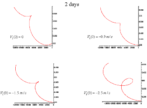
Figure 2: Possible artificial trajectories at $22^{o}N,\,$$b_{0}=10^{-6}\,s^{-1},\,$ $c_{0}=10^{-1},\,$$M(0)=N(0)=10^{-9},\,$$V_{2}(0)=0$ (in corresponding units) [2]

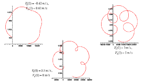
Figure 3: Possible artificial trajectories at $22^{o}N,\,b_{0}=10^{-5}\,s^{-1},\,$ $c_{0}=10^{-1},\,$$M(0)=N(0)=10^{-9}$ (in corresponding units) [2]

It is possible to compute the position $(x_{1},x_{2})$ of the trajectory based on the system (3.8 – 3.15), (3.5) by applying ODE integrators. However, the difference between the numerical trajectory and points on the curve (4.1), (4.2) for the physical values of parameters is very little. For example, for the initial data $a(0)=10^{-5}s^{-1},\,b(0)=5\cdot 10^{-5}s^{-1},\,A(0)=10^{-9}\,(N\cdot m^{-2})^{(\gamma-1)/\gamma}\cdot m^{-2},\,N(0)=10^{-3}\,(N\cdot m^{-2})^{(\gamma-1)/\gamma}\cdot m^{-1},\,M(0)=2\,N(0),\,V_{1}(0)=-1\cdot m\cdot s^{-1},\,V_{2}(0)=1\cdot m\cdot s^{-1},\,x_{1}(0)=x_{2}(0)=0,$ the difference in positions after three days is about $20\,km$ (see Fig.4). (Here, the radius of typhoon is taken as 300 $km,$ the difference between the pressure at the center of typhoon and the ambient pressure is $10^{4}\,Pa,$ the constant $c_{0}$ is estimated as $10^{-1}$). Therefore, basically, there is no reason to get the solution curves by applying numerical integration for (3.8 – 3.15) and (3.5) instead of using explicit formulas (4.1) and (4.2).

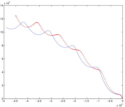
Figure 4: Difference between trajectories corresponding to the exact equilibrium point (solid line) and in a vicinity of equilibrium (dashed line) within three days

5 Examples of analysis of real trajectories

Assume initial conditions are known, one can integrate the system (3.8)– (3.15), (3.5). But these initial conditions include the height-averaged physical quantities such as divergency $a(0),$ vorticity $b(0),$ parameters $A(0),$ $M(0),$ $N(0),$ (relating to the pressure field), and the initial velocity $V(0).$ It is not clear how to measure these quantities. The only widely available information is positions of the typhoon eye. Thus, we try to fit the parameters using the formulas (4.1) and (4.2). However, it needs to assume that the vortex is at its conservative phase.

We use the following algorithm: at the first step, we choose three successive points of trajectory ($(x_{1}(t_{0}),x_{2}(t_{0})),(x_{1}(t_{1}),x_{2}(t_{1})),(x_{1}(t_{2}),x_{2}(t_{2}))$). Formulas (4.1), (4.2) give a system of four linear algebraic equations with respect to $V_{1}(0),\,V_{2}(0),\,c_{0}M(0),\,c_{0}N(0).$ The parameter $b_{0}$ is free. The value of the Coriolis parameter $l$ is calculated at the initial point $(x_{1}(t_{0}),x_{2}(t_{0})).$ The second step is to choose the parameter $b_{0}.$ If we deal with historical trajectory, $b_{0}$ can be fitted so that the artificial trajectory coincides with the real one as long as possible. As we should show, the coincidence sometime lasts for several days.

In practice, we can compute $b_{0},$ for example, from the condition

$$V_{1}(0)=\bar{V}_{1}(0),$$ (5.1)

$$V_{2}(0)=\bar{V}_{2}(0),$$ (5.2)

where $\bar{V}_{i}(0)=\frac{x_{i}(t_{1})-x_{i}(t_{0})}{t_{1}-t_{0}},\,i=1,2.$ However, (5.1) and (5.2) give different values of $b_{0}$ basically.

Let us estimate all possible values of parameter $b_{0}$ at the equilibrium point. As it follows from (3.9), $b_{0}$ is a root of the quadratic equation

$$b_{0}^{2}-lb_{0}-2c_{0}A_{0}=0,$$

therefore, $b_{0}\approx-\frac{2c_{0}A_{0}}{l}.$ for $c_{0}A_{0}<<l^{2}$. If we further assume $A_{0}=10^{-9},\,c_{0}=10^{-1},\,l=10^{-4},$ $b_{0}\approx-2\cdot 10^{-6}.$ Thus, to be physically meaningful, we can assume $|b_{0}|\leq 10^{-5}$ and bear in mind that this value is essentially negative.

Thus, if the set of three points is not able provide an appropriate value of $b_{0},$ the prediction is considered as a failure. We need to shift these three points until we get a definite value of $b_{0}$ that can be used for the weather forecast.

We consider three successive points as suitable candidates for a forecast if equations (5.1) and (5.2) have roots $b_{01}$ and $b_{02}$ in the interval $|b_{0}|\leq 10^{-5}$ respectively and $|b_{01}-b_{02}|<\varepsilon,$ with $\varepsilon$ sufficiently small. In this case, we chose $b_{0}$ as the mean of $b_{01}$ and $b_{02}.$

In the next, we give two examples of analysis of the real tropical typhoon tracks.

5.1 Man Yi

Let us consider a recent typhoon of the West Pacific region, Man Yi (4 category, July 8-15, 2007). The historic trajectory and observational data are given on Figs.5 and 6 [18]. Remark that the numeration cited in Fig.6 includes certain intermediate points (like 1A, 2A, etc). Here, We did numerate the intermediate points as in Fig. 6, instead, we adopt successive numeration in our examples.

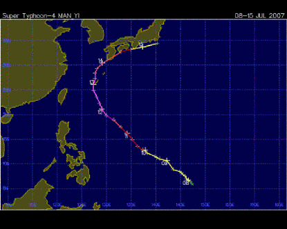
Figure 5: The Man Yi trajectory [18]

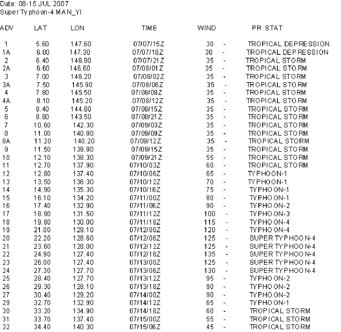
Figure 6: The Man Yi data [18]

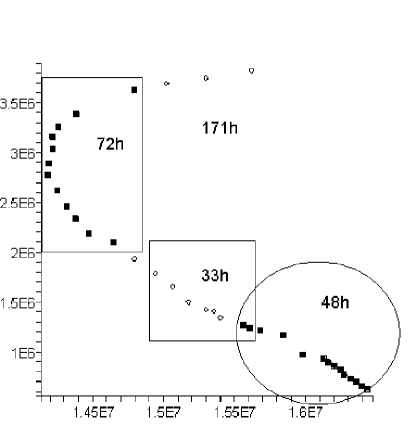
Figure 7: The Man Yi trajectory (observational data) with analyzed regions

5.1.1 Historical trajectory: fitting averaged vorticity

By analyzing the trajectory of the typhoon Man Yi, we found that it is possible to fit $b_{0}$ so that there is a good coincidence with the artificial trajectory given by formulas (4.1) and (4.2) in three different regions (Fig.7). Here and below graphs, the diamond shape points represent the observational path of tropical typhoon and solid lines represent the analytic results; the first three points of trajectories, where the points and line coincide, are used for the parameters estimation. The first region corresponds to the first 14 points on Fig.7 (the total duration is 48 hours, the ”tropical storm” stage). Fig.11 shows the prediction for point 1 to 9 (18 hours), Fig.11 - for point 1 to 14 (48 hours). Here, we get $b_{0}=2.236198023\cdot 10^{-6}\,s^{-1}.$ The second region on Fig.7 corresponds to points 12 - 19 (33 hours, ”tropical storm - typhoon 1”, Fig.11). At this region, the vortex is developing, thus we can not consider it as a stable one. Generally, making predictions according formulas (4.1), (4.2) may not give good results for unstable regions. Nevertheless, these formulas with $b_{0}=-1.8\cdot 10^{-5}\,s^{-1}$ still gives a satisfactory coincidence for the real and artificial trajectories. The third region that we analyze is from point 22 to 34, which lasts for 72 hours. In this case, the typhoon is developing from 3th to 4th stage and then decays. We get $b_{0}=-1\cdot 10^{-5}$ and obtain a very good coincidence for the 3 day period.

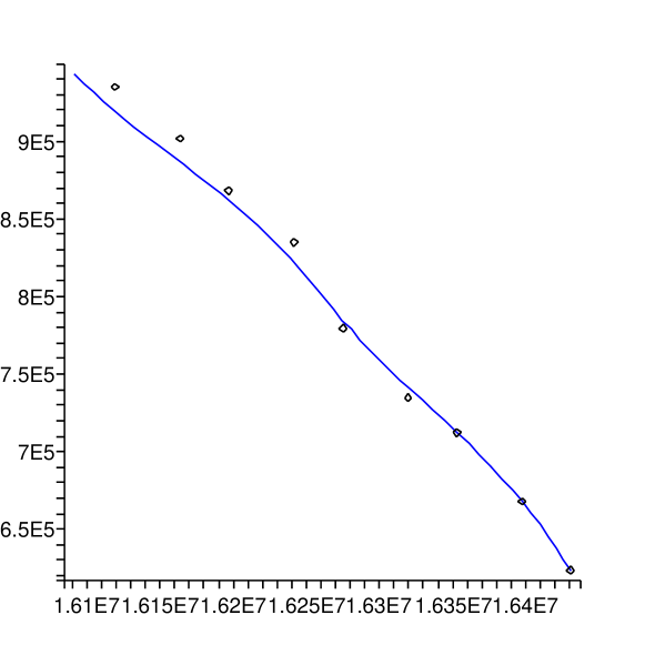
Figure 8: The first 9 points (18 hours). Here and below dots corresponds to observational data, solid line represents analytic results

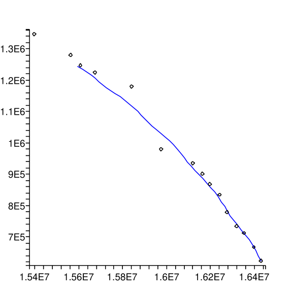
Figure 9: The first 14 points (48 hours)

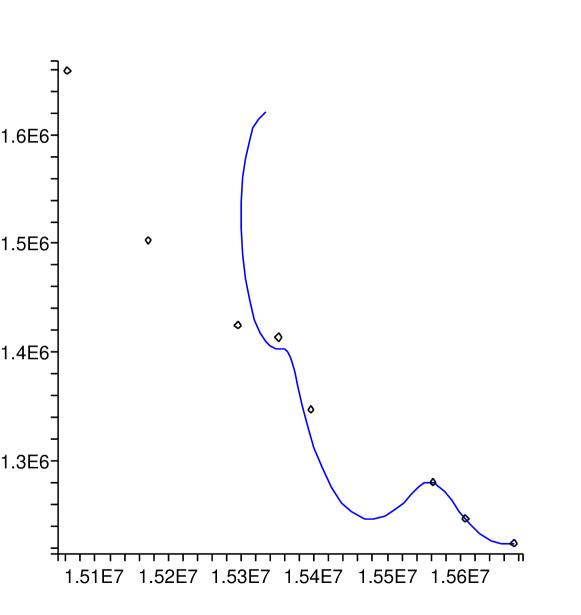
Figure 10: 12–19 points (33 hours)

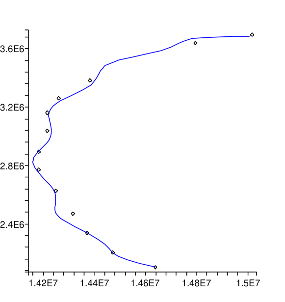
Figure 11: 22–34 points (72 hours)

5.1.2 Attempt of a forecast in real time

Now, suppose that that we do not know the track of the whole trajectory in advance and try to find $b_{0}$ to compare its value found from (5.1) and (5.2). It is worth to note that one may propose other methods to find the averaged vorticity. This will be a subject of our further investigations. Let us mention that one can consider the neural network approaches for this direction[17].

If we set $\varepsilon=2\cdot 10^{-6},$ we get only two appropriate three point sets: one of them begins from the 21th point and gives a very good prediction (Fig.11), here $b_{0}\approx 1\cdot 10^{-5}\,s^{-5}$). The other one predicts a loop beginning from the point 7 (see Fig.13). Thus, one can assume that at the 9th point, the vortex had gone through an exterior force. It constrains the trajectory to change the direction of its path.

If we weaken the requirement for accuracy and set $\varepsilon=3\cdot 10^{-6},$ we get one more three point set, beginning from point 24. In the latter case, the artificial trajectory gives a true direction. But comparing with the exact track, the artificial trajectory outgoing from the 21th point (Fig.13) is bad. However, the spread of positions is inside of the annual mean diameter of the 33 percent strike probability region for 36 hours [4].

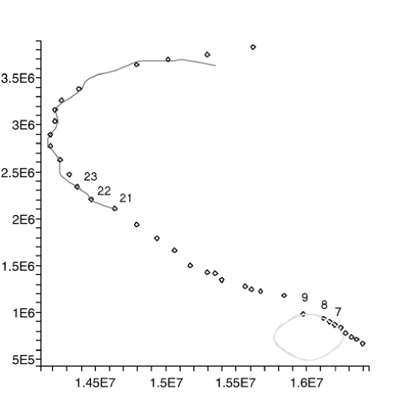
Figure 12: $\varepsilon=2\cdot 10^{-6}$: potential loop

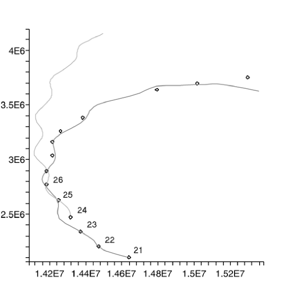
Figure 13: $\varepsilon=3\cdot 10^{-6}$: two best predictions

5.2 Parma

Now we consider the example of typhoon with a looping trajectory, Parma, 20-31 October, 2003, Fig.14, Fig.15.

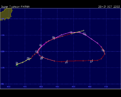
Figure 14: The Parma trajectory [18]

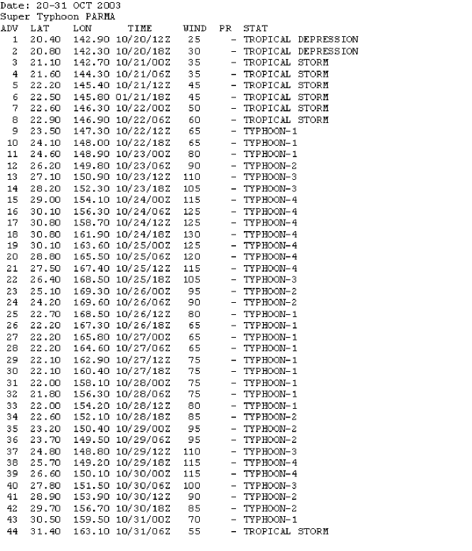
Figure 15: The Parma data [18]

Fig. 17 presents the comparison of real trajectory within 78 hours of the typhoon in its conservative phase. The parameter $b_{0}=-6.1116738183\cdot 10^{-5}s^{-1}$ is fitted for all points of trajectory according the historical data. Fig. 17 presents a forecast for a long period (144 h.) based on the data for 12 hours. We can see that the forecast gives the true qualitative behavior of the trajectory, the loop. This loop was deformed by a steering flow.

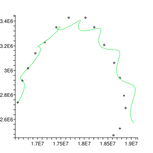
Figure 16: The Parma trajectory from       10 to 25th point (78 hours)

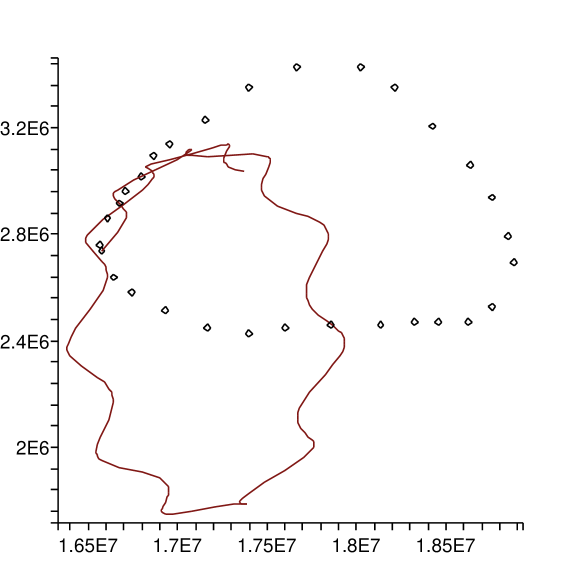
Figure 17: Forecast for 144 hours based on 10-12 points (12 hours))

6 The role of surface friction

It is well known that the typhoons basically do not last for a long time over a dry land. The key point is the significant increasing of the dry friction when the typhoon goes to the land. Now, let us add the damping term $-k{\bf U}$ in the right hand side of first equation (2.8), where $k$ is a nonnegative function of coordinates. For simplicity, we assume that $k$ is a constant. Therefore instead of (3.9),(3.10), we get

$$\dot{a}+a^{2}-b^{2}+lb+2c_{0}A=-ka,$$ (6.1)

$$\dot{b}+2ab-la=-kb,$$ (6.2)

equations (3.8),(3.11) – (3.15) do not change.

System (3.8), (6.1), (6.2) is closed. However, it does not encounter any equilibrium for $A\neq 0.$ Therefore, it is not possbile to find a stable domain of low pressure from this system. Fig.18 and 19 demonstrate the break-up of the stable equilibrium for $k>0.$ Computer simulations are made for initial data $A_{0}=10^{-9},$ $a(0)=0,$ $b(0)=-2\cdot 10^{-6},$ $l=10^{-4},$ $c_{0}=0.1$ (in respective units). Fig. 18 presents the phase portrait of the system (3.8), (6.1), and (6.2) for $k=0.$ In this case, a stable equilibrium exists on the phase plane. Fig. 19 shows the collapse of vortex for $k>0:$ the vortex strehgth slightly intensifies, whereas the motion becomes significantly convergent eventually. Here, initial data are the same as in Fig.18, $k=3\cdot 10^{-5}.$

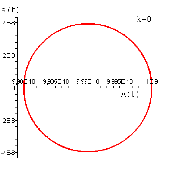
Figure 18: The phase portrait of (3.8),       (6.1),(6.2) for $k=0.$

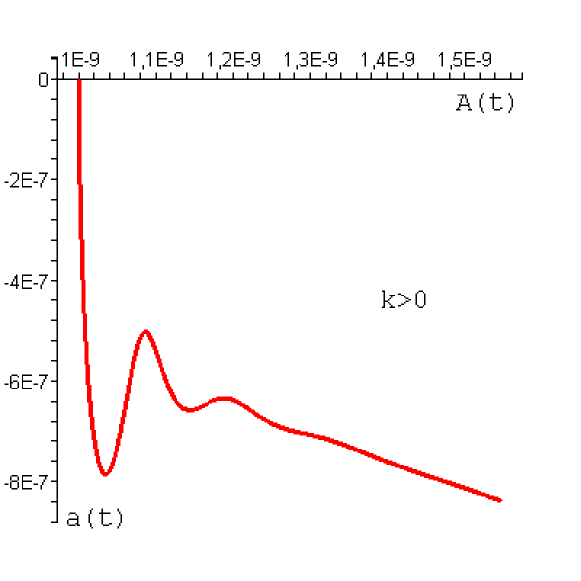
Figure 19: The same an in Fig.18 for $k=3\cdot 10^{-5},$ computations are made for 3 days.

Thus, if we wish to obtain a stable vortex along with the surface friction, we have to consider some additional phenomenon such as vertical advection (see [19]) in this context).

Note that the system (3.8), (6.1), (6.2) is very interesting from the mathematical point of view. It has a complex equilibrium at the origin and there is a possibility of existence of a strange attractor for certain values of parameters.

7 Discussion

In this paper, we show that the behavior of the developed tropical cyclone trajectory is determinated by exterior and inner parameters; the trajectory is a superposition of two circular motions: one has period $2\pi/l,$ the other one has period $2\pi/b_{0}.$

Our previous conclusion that the trajectories for both barotropic and baroclinic models are governed by the same system of coefficient-equations seems conflict with the fact that baroclinicity has a strong relation with the cyclone formation. About this point, we would like to clarify that the cyclone formation in our paper only refers to the conservative (or near conservative) phase of the atmosphere vortex development. Indeed, the evidence about the velocity in a linear form (3.1) can be confirmed by the observational data which is collected as the developed typhoon is close to its center. As it shows in (Fig.1), at the stage of the vortex formation, the velocity may not to be linear. Therefore, we claim that we find a “toy” solution for a very complicated system to describe the processes of formation and decay of cyclones for which an analytical solution is barely to be obtained. It worth to remark again that the term “barotropicity” in our paper is only restricted to describe the bidimensional framework. i.e. the term “barotropicity” is used with a hidden meaning of “taking an average over the height”. In the physical 3D space, the flow does not have to be barotropic.

Our arguments can be verified from other researchers, for examples, in [20], it says “The curvature of storm track is determined by a set of ‘controlling parameters’ related to the storm characteristics and ambient atmospheric circulation. These controlling parameters include the speed of storm (${\bf V}(0)$ in our notation), storm intensity ($b(0)$), size ($A(0)$), the Coriolis parameter ($l$), ambient atmospheric pressure field ($M(0),N(0)$) and surface friction ($k$)”. Also in [3], it says that “In a barotropic framework, a tropical cyclone is basically “steered” by the surrounding flow ($V(0),M(0),N(0)$), but its movement is modified by the Coriolis force and the horizontal vorticity gradient of the surrounding flow.”

Certainly, it would be naive to claim that our model provides a better weather forecast for the typhoon trajectory than those modern models using numerical simulations. Firstly, the formula is derived under the assumption that the vortex is at stable phase, but, this assumption hardy holds for the real weather forecast. Therefore, we only can deal with oscillations near the equilibrium point at most in our model. Secondly, the only variables that we feed in the equations of thermodynamic parameters are initial data from real cases. However, as the vortex moves, it may experience a forcing of baric fields, which may skew its trajectory significantly. Thus, generally, we can only expect to get the reproduction of the trajectories qualitatively, i.e., to predict a turning of the track without indicating the exact position of the vortex. Finally, we do not take into consideration the curvilinear geometry of the Earth surface. Therefore, only in a vicinity of an initial point, the linearization does not result in a big distortion. The inclusion of the $\beta$ - effect does not give an exact solution with respect to the stable vortex (for approximative solutions, see [21]).

However, as in [4], even high-quality weather forecast models may not be reliable due to its uncertainty about the initial conditions or for some other unknown reasons. Thus, operational weather forecasters still need to judge whether or not the prediction results should be taken into consideration to build an official weather forecast in their daily work. Therefore, it is helpful to have a complimentary tool to aid other existing models for the typhoon trajectory prediction. Our model seems very simple comparing with models used for the numerical weather forecast. However, it is very useful since it can be used to explain the trajectory behavior, predict the direction of the trajectory and the loop formation as well.

Our models can be further refined in two aspects: doing analytical refinement of the model and searching a better way for parameters-fitting. We conjecture that it is possible to obtain some solutions with analytical format for the Navier-Stokes system in spherical coordinates. Then we could include the $\beta$ - drift in our model and release the requirement that the solutions need to be bound around the neighborhood of the center of typhoon. The natural question arising in the parameters-fitting method is: can we actually use the average vorticity $b_{0}$ as a measurement of predictability in the model? As it is mentioned in the previous sections, even feeding with the real data for the average vorticity $b_{0},$ one can only get approximate predication for the trajectory behavior. The quality of the predication strongly depends on the ambient meteorological fields, which are responsible for the steering effect. In particular, the“regularity” of the ambient meteorological fields seems to be a very crucial factor for the trajectory tracing. However, it can not be obtained only through analyzing the equations of trajectories. Thus, to improve the predictability and accuracy for our model, we need to combine our method with the analysis of available meteorological data and include other theorems like statistical moments (see in this context [22]) and neural networks [23], [17] in our model.

ACKNOWLEDGMENTS

This work was supported by the National Science Council of Taiwan under Grand Nos. NSC 96-2911-M001-003-MY3 and NSC 96-2112-M017-001-MY3 and National Center for Theoretical Sciences in Taiwan. O.Rozanova was also supported by the special program of the Ministry of Education of the Russian Federation ”The development of scientific potential of the Higher School”, project 2.1.1/1399.

References

- [1] Gray W.M.(1968) Global view of the origin of tropical disturbances and storms, Mon.Weath.Rev., v.96, 669-700.
- [2] Rozanova, O.S. (2004) Note on a typhoon eye trajectory. Regular and Chaotic Dynamics, v.9, n.2, pp.129-142.
- [3] Chan, J.C.L.(2005) The physics of tropical cyclone motion. Annual review of fluid mechanics. 37 99–128 Annual Reviews, Palo Alto, CA.
- [4] Weber, H.C.(2005) Probabilistic prediction of tropical cyclones. Part I: Position.Monthly Weather Review, v.133, pp.1840-1852.
- [5] Dolzhanskii, F.V., Krymov, V.A., Manin, D.Yu. (1990) Stability and vortex structures of quasi-two-dimensional shear flows Sov.Phys.Usp., 33(7), 495-520.
- [6] Pedlosky, J. (1979) Geophysical fluid dynamics, Springer-Verlag, New York.
- [7] Landau, L.D.; Lifshits, E.M.(1987), Fluid mechanics. 2nd ed. Volume 6 of Course of Theoretical Physics. Transl. from the Russian by J. B. Sykes and W. H. Reid. (English) Oxford etc.: Pergamon Press. XIII, 539 p.
- [8] Alishaev, D.M.(1980), On dynamics of two-dimensional baroclinic atmosphere Izv.Acad.Nauk, Fiz.Atmos.Oceana,16, N 2, 99-107.
- [9] Obukhov, A.M.(1949), On the geostrophical wind Izv.Acad.Nauk (Izvestiya of Academie of Science of URSS), Ser. Geography and Geophysics,XIII, 281-306.
- [10] Bulatov, V.V., Vladimirov, Yu.V., Danilov, V.G., Dobrokhotov, S.Yu.(1994) Calculations of hurricane trajectory on the basis of V. P. Maslov hypothesis. Dokl. Akad. Nauk, Ross. Akad. Nauk 338, No.1, 102-105.
- [11] Bulatov, V.V.; Vladimirov, Yu.V.; Danilov, V.G.; Dobrokhotov, S.Yu.(1994) On motion of the point algebraic singularity for two-dimensional nonlinear equations of hydrodynamics Math. Notes 55, No.3, 243-250; translation from Mat. Zametki 55, No.3, 11-20.
- [12] Dobrokhotov, S.Yu., Shafarevich, A.I., Tirozzi, B. (2006) The Cauchy-Riemann conditions and localized asymptotic solutions of linearized equations in shallow water theory, Appl.Math.Mech. 69 (5), 720-725.
- [13] Rozanova, O.S. (2003):On classes of globally smooth solutions to the Euler equations in several dimensions. In: Hyperbolic problems: theory, numerics, applications, 861–870, Springer, Berlin.
- [14] Rozanova, O.S. (2003), Application of integral functionals to the study of the properties of solutions to the Euler equations on riemannian manifolds, J.Math.Sci. 117(5), 4551–4584.
- [15] Rozanova, O.S.(2007), Formation of singularities of solutions to the equations of motion of compressible fluid subjected to external forces in the case of several spatial variables, J.Math.Sci. 143 (4).
- [16] Sheets, R.C.(1981)On the structure of hurricanes as revealed by research Aircraft data, In: Intense atmospheric vortices. Proceedings of the Joint Simposium (IUTAM/IUGC) held at Reading (United Kingdom) July 14-17, 1981. Edited by L.Begtsson and J.Lighthill, pp.33-49.
- [17] Reutskiy, S., Tirozzi, B. (2007) Forecast of the trajectory of the senter of typhoons and the Maslov decomposition, Russian Journal of Mathematical Physics, 14(2), 232-237.
- [18] http://weather.unisys.com/hurricane/index.html
- [19] Fujita Yashima, H., Rozanova, O.S., Stationary solution to the air motion equa-tions in the lower part of typhoon (2007) J.of Applied and Industrial Mathematics, 1 (2), 1-22.
- [20] Xu, X., Xie, L., Zhang, X., Yao, W. (2006) A mathematical model for forecasting tropical cyclone tracks. Nonlinear Analysis: Real World Applications 7 211-224.
- [21] Dobrokhotov, S.Yu.(1999) Hugoniot-Maslov chains for solitary vortices of the shallow water equations. I: Derivation of the chains for the case of variable Coriolis forces and reduction to the Hill equation, Russ. J. Math. Phys. 6, No.2, 137-173.
- [22] Danilov, V., Omelyanov, S., Rozenknop, D.,(2002)Calculations of the hurricane eye motion based on singularity propagation theory, Electron. J. Diff. Eqns., Vol. 2002, No. 16, pp. 1-17.
- [23] Tirozzi,B., Puca,S., Pittalis, S., Bruschi, A., Morucci, S., Ferraro, E., Corsini,S. (2005) Neural Networks and Sea Time Series, Reconstruction and Extreme event analysis, MSSET, Birkhauser, Boston.