Resummation of transverse energy in vector boson and Higgs boson production at hadron colliders

Abstract:

We compute the resummed hadronic transverse energy ($E_{T}$) distribution due to initial-state QCD radiation in vector boson and Higgs boson production at hadron colliders. The resummed exponent, parton distributions and coefficient functions are treated consistently to next-to-leading order. The results are matched to fixed-order calculations at large $E_{T}$ and compared with parton-shower Monte Carlo predictions at Tevatron and LHC energies.

1 Introduction

The QCD radiation from incoming partons forms an inescapable component of the final state in all hard scattering processes at hadron colliders. This radiation leads to hadron formation that complicates the interpretation of events in a number of ways: by generating extra jets, by contaminating other jets, by modifying event shapes and global observables, and by changing the distributions of the products of the hard process. This last effect has been studied in great detail for the processes of electroweak boson production, with the result that the transverse momentum and rapidity distributions of W, Z and Higgs bosons at the Tevatron and LHC are predicted with good precision. The predictions for the transverse momentum ($q_{T}$) distributions in particular include resummation of terms enhanced at small $q_{T}$ to all orders in $\alpha_{\mathrm{S}}$, matched with fixed-order calculations at higher $q_{T}$ values. The transverse momentum of the boson arises (neglecting the small intrinsic transverse momenta of the partons in the colliding hadrons) from its recoil against the transverse momenta of the radiated partons: $q_{T}=|\mbox{\boldmath$q$}_{T}|$ where

$$\mbox{\boldmath$q$}_{T}=-\sum_{i}\mbox{\boldmath$p$}_{Ti}\;.$$ (1)

The resummation of enhanced terms therefore requires a sum over emissions $i$ subject to the constraint (1), which is most conveniently carried out in the transverse space of the impact parameter $b$ Fourier conjugate to $\mbox{\boldmath$q$}_{T}$:

$$\delta(\mbox{\boldmath$q$}_{T}+\sum\mbox{\boldmath$p$}_{Ti})=\frac{1}{(2\pi)^{2}}\int d^{2}\mbox{\boldmath$b$}\,{\rm e}^{i\mbox{\boldmath\scriptsize$q$}_{T}\cdot\mbox{\boldmath\scriptsize$b$}}\prod_{i}{\rm e}^{i\mbox{\boldmath\scriptsize$p$}_{Ti}\cdot\mbox{\boldmath\scriptsize$b$}}\;.$$ (2)

One then finds that the cumulative distribution in $b=|\mbox{\boldmath$b$}|$ contains terms of the form $\alpha_{\mathrm{S}}^{n}\ln^{p}(Qb)$, where $Q$ is the scale of the hard process, set in this case by the mass of the electroweak boson, and $p\leq 2n$. These terms, which spoil the convergence of the perturbation series at large $b$, corresponding to small $q_{T}$, are found to exponentiate [4, 5, 6, 7, 8, 9]: that is, they can be assembled into an exponential function of terms that are limited to $p\leq n+1$. This resummation procedure improves the convergence of the perturbation series at large values of $b$ and hence allows one to extend predictions of the $q_{T}$ distribution to smaller values.

Together with its vector transverse momentum $\mbox{\boldmath$p$}_{Ti}$, every emission generates a contribution to the total hadronic transverse energy of the final state, $E_{T}$, which, neglecting parton masses, is given by

$$E_{T}=\sum_{i}|\mbox{\boldmath$p$}_{Ti}|\;.$$ (3)

To first order in $\alpha_{\mathrm{S}}$ (0 or 1 emissions) this quantity coincides with $q_{T}$, but they differ in higher orders. In particular, at small $q_{T}$ there is the possibility of vectorial cancellation between the contributions of different emissions, whereas this cannot happen for the scalar $E_{T}$. Thus the distribution of $E_{T}$ vanishes faster at the origin, and its peak is pushed to higher values. To resum these contributions at small $E_{T}$, one should perform a one-dimensional Fourier transformation and work in terms of a ‘transverse time’ variable $\tau$ conjugate to $E_{T}$:

$$\delta(E_{T}-\sum|\mbox{\boldmath$p$}_{Ti}|)=\frac{1}{2\pi}\int d\tau\,{\rm e}^{-iE_{T}\tau}\prod_{i}{\rm e}^{i|\mbox{\boldmath\scriptsize$p$}_{Ti}|\tau}\;.$$ (4)

Since the matrix elements involved are the same, one finds a similar pattern of enhanced terms at large $\tau$ as was the case for large $b$: terms of the form $\alpha_{\mathrm{S}}^{n}\ln^{p}(Q\tau)$ with $p\leq 2n$, which arise from an exponential function of terms with $p\leq n+1$. Evaluation of the exponent to a certain level of precision (leading-logarithmic, LL, for $p=n+1$, next-to-leading, NLL, for $p=n$, etc.) resums a corresponding class of enhanced terms and extends the validity of predictions to lower values of $E_{T}$.

The resummation of $E_{T}$ in this way has received little attention since the first papers on this topic, over 20 years ago [10, 11, 12]. This is surprising, as most of the effects of QCD radiation from incoming partons mentioned above depend on this variable rather than $q_{T}$. A possible reason is that, unlike $q_{T}$, $E_{T}$ also receives an important contribution from the so-called underlying event, which is thought to arise from secondary interactions between spectator partons. At present this can only be estimated from Monte Carlo simulations that include multiple parton interactions (MPI). Nevertheless it is worthwhile to predict as accurately as possible the component coming from the primary interaction, which carries important information about the hard process. For example, we expect the $E_{T}$ distributions in Higgs and vector boson production to be different, as they involve primarily gluon-gluon and quark-antiquark annihilation, respectively. Accurate estimates of the primary $E_{T}$ distribution are also important for improving the modelling of the underlying event.

In the present paper we extend the resummation of $E_{T}$ in vector boson production to next-to-leading order (NLO) in the resummed exponent, parton distributions and coefficient functions, and present for the first time the corresponding predictions for Higgs boson production. In Section 2 the resummation procedure is reviewed and extended to NLO; results on the resummed component are presented in Sect. 3. This component alone is not expected to describe the region of larger $E_{T}$ values, of the order of the boson mass; in Sect. 4 we describe and apply a simple procedure for including the unresummed component at order $\alpha_{\mathrm{S}}$. Section 5 presents $E_{T}$ distributions generated using the parton shower Monte Carlo programs HERWIG [13] and Herwig++ [14], which are compared with the analytical results and used to estimate of the effects of hadronization and the underlying event. Our conclusions are summarized in Sect. 6. Appendix A gives mathematical details of a comparison between the resummation of the transverse energy $E_{T}$ and transverse momentum $q_{T}$ and Appendix B shows results for the LHC at lower centre-of-mass energy.

2 Resummation method

2.1 General procedure

Here we generalize the results of ref. [11] to NLO resummation. The resummed component of the transverse energy distribution in the process $h_{1}h_{2}\to FX$ at scale $Q$ takes the form

$$\left[\frac{d\sigma_{F}}{dQ^{2}\;dE_{T}}\right]_{{\rm res.}} = \frac{1}{2\pi}\sum_{a,b}\int_{0}^{1}dx_{1}\int_{0}^{1}dx_{2}\int_{-\infty}^{+\infty}d\tau\;{\rm e}^{-i\tau E_{T}}\;f_{a/h_{1}}(x_{1},\mu)\;f_{b/h_{2}}(x_{2},\mu)$$ (5)

$$\cdot W_{ab}^{F}(x_{1}x_{2}s;Q,\tau,\mu)$$

where $f_{a/h}(x,\mu)$ is the parton distribution function (PDF) of parton $a$ in hadron $h$ at factorization scale $\mu$, taken to be the same as the renormalization scale here. In what follows we use the ${\overline{\rm MS}}$ renormalization scheme. As mentioned earlier, to take into account the constraint that the transverse energies of emitted partons should sum to $E_{T}$, the resummation procedure is carried out in the domain that is Fourier conjugate to $E_{T}$, using Eq. (4). The transverse energy distribution (5) is thus obtained by performing the inverse Fourier transformation with respect to the transverse time, $\tau$. The factor $W_{ab}^{F}$ is the perturbative and process-dependent partonic cross section that embodies the all-order resummation of the large logarithms $\ln(Q\tau)$. Since $\tau$ is conjugate to $E_{T}$, the limit $E_{T}\ll Q$ corresponds to $Q\tau\gg 1$.

As in the case of transverse momentum resummation [15], the resummed partonic cross section can be written in the following universal form:

$$W_{ab}^{F}(s;Q,\tau,\mu) = \sum_{c}\int_{0}^{1}dz_{1}\int_{0}^{1}dz_{2}\;C_{ca}(\alpha_{\mathrm{S}}(\mu),z_{1};\tau,\mu)\;C_{{\bar{c}}b}(\alpha_{\mathrm{S}}(\mu),z_{2};\tau,\mu)\;\delta(Q^{2}-z_{1}z_{2}s)$$ (6)

$$\cdot \sigma_{c{\bar{c}}}^{F}(Q,\alpha_{\mathrm{S}}(Q))\;S_{c}(Q,\tau)\;\;.$$

Here $\sigma_{c{\bar{c}}}^{F}$ is the cross section for the partonic subprocess $c+{\bar{c}}\to F$, where $c,{\bar{c}}=q,{\bar{q}}$ (the quark $q_{f}$ and the antiquark ${\bar{q}}_{f^{\prime}}$ can possibly have different flavours $f,f^{\prime}$) or $c,{\bar{c}}=g,g$. The term $S_{c}(Q,\tau)$ is the quark $(c=q)$ or gluon $(c=g)$ Sudakov form factor. In the case of $E_{T}$ resummation, this takes the form [11, 12]

$$S_{c}(Q,\tau)=\exp\left\{-2\int_{0}^{Q}\frac{dq}{q}\left[2A_{c}(\alpha_{\mathrm{S}}(q))\;\ln\frac{Q}{q}+B_{c}(\alpha_{\mathrm{S}}(q))\right]\left(1-{\rm e}^{iq\tau}\right)\right\}\;,$$ (7)

with $c=q$ or $g$. The functions $A_{c}(\alpha_{\mathrm{S}}),B_{c}(\alpha_{\mathrm{S}})$, as well as the coefficient functions $C_{ab}$ in Eq. (6), contain no $\ln(Q\tau)$ terms and are perturbatively computable as power expansions with constant coefficients:

$$A_{c}(\alpha_{\mathrm{S}}) = \sum_{n=1}^{\infty}\left(\frac{\alpha_{\mathrm{S}}}{\pi}\right)^{n}A_{c}^{(n)}\;\;,$$ (8)

$$B_{c}(\alpha_{\mathrm{S}}) = \sum_{n=1}^{\infty}\left(\frac{\alpha_{\mathrm{S}}}{\pi}\right)^{n}B_{c}^{(n)}\;\;,$$ (9)

$$C_{ab}(\alpha_{\mathrm{S}},z) = \delta_{ab}\,\delta(1-z)+\sum_{n=1}^{\infty}\left(\frac{\alpha_{\mathrm{S}}}{\pi}\right)^{n}C_{ab}^{(n)}(z)\;\;.$$ (10)

Thus a calculation to NLO in $\alpha_{\mathrm{S}}$ involves the coefficients $A_{c}^{(1)}$, $A_{c}^{(2)}$, $B_{c}^{(1)}$, $B_{c}^{(2)}$ and $C_{ab}^{(1)}$. All these quantities are known for both the quark and gluon form factors and associated coefficient functions. Knowledge of the coefficients $A^{(1)}$ leads to the resummation of the leading logarithmic (LL) contributions at small $E_{T}$, which in the differential distribution are of the form $\alpha_{\mathrm{S}}^{n}\ln^{p}(Q/E_{T})/E_{T}$ where $p=2n-1$. The coefficients $B^{(1)}$ give the next-to-leading logarithmic (NLL) terms with $p=2n-2$, $A^{(2)}$ and $C^{(1)}$ give the next-to-next-to-leading logarithmic (N²LL) terms with $p=2n-3$, and $B^{(2)}$ gives the N³LL terms with $p=2n-4$. With knowledge of all these terms, the first term neglected in the resummed part of the distribution is of order $\alpha_{\mathrm{S}}^{3}\ln(Q/E_{T})/E_{T}$.

In general the coefficient functions in Eq. (6) contain logarithms of $\mu\tau$, which are eliminated by a suitable choice of factorization scale. To find the optimal factorization scale, we note that, to NLL accuracy,

$$\int_{0}^{Q}\frac{dq}{q}\ln^{p}q\left(1-{\rm e}^{iq\tau}\right)\simeq\int_{i\tau_{0}/\tau}^{Q}\frac{dq}{q}\ln^{p}q\;,$$ (11)

where $\tau_{0}=\exp(-\gamma_{E})=0.56146\ldots$, $\gamma_{E}$ being the Euler-Mascheroni constant. Therefore the effective lower limit of the soft resummation is $i\tau_{0}/\tau$, and the parton distributions and coefficient functions should be evaluated at this scale. However, evaluation of parton distribution functions at an imaginary scale using the standard parametrizations is not feasible. We avoid this by noting that

$$f_{a/h}(x,q^{\prime})=\sum_{b}\int_{x}^{1}\frac{dz}{z}U_{ab}(z;q^{\prime},q)f_{b/h}(x/z,q)$$ (12)

where $U_{ab}$ is the DGLAP evolution operator. Therefore

$$f_{a/h}(x,i\mu)=\int_{x}^{1}\frac{dz}{z}U_{ab}(z;i\mu,\mu)f_{b/h}(x/z,\mu)$$ (13)

where the evolution operator $U_{ab}(z;i\mu,\mu)$ is given to NLO by

$$U_{ab}(z;i\mu,\mu)=\delta_{ab}+\frac{i}{2}\alpha_{\mathrm{S}}(\mu)\,P_{ab}(z)\;,$$ (14)

$P_{ab}(z)$ being the leading-order DGLAP splitting function. Similarly, in the coefficient functions we can write $\alpha_{\mathrm{S}}(i\mu)$ in terms of $\alpha_{\mathrm{S}}(\mu)$ using the definition of the running coupling:

$$\int_{\mu}^{i\mu}\frac{d\alpha_{\mathrm{S}}}{\beta(\alpha_{\mathrm{S}})}=2\int_{\mu}^{i\mu}\frac{dq}{q}=i\pi$$ (15)

where $\beta(\alpha_{\mathrm{S}})=-b\alpha_{\mathrm{S}}^{2}+{\cal O}(\alpha_{\mathrm{S}}^{3})$, so that

$$\alpha_{\mathrm{S}}(i\mu)=\alpha_{\mathrm{S}}(\mu)-i\pi b[\alpha_{\mathrm{S}}(\mu)]^{2}+{\cal O}(\alpha_{\mathrm{S}}^{3})\;.$$ (16)

Furthermore, as the expressions (5) and (6) are convolutions, we can transfer the extra terms from (13) into the coefficient functions to obtain

$$W_{ab}^{F}(s;Q,\tau) = \sum_{c}\int_{0}^{1}dz_{1}\int_{0}^{1}dz_{2}\;\widetilde{C}_{ca}(\alpha_{\mathrm{S}}(\tau_{0}/\tau),z_{1})\;\widetilde{C}_{{\bar{c}}b}(\alpha_{\mathrm{S}}(\tau_{0}/\tau),z_{2})\;\delta(Q^{2}-z_{1}z_{2}s)$$ (17)

$$\cdot \sigma_{c{\bar{c}}}^{F}(Q,\alpha_{\mathrm{S}}(Q))\;S_{c}(Q,\tau)$$

where

$$\widetilde{C}_{ca}(\alpha_{\mathrm{S}}(\mu),z)=\sum_{d}\int_{z}^{1}\frac{dz^{\prime}}{z^{\prime}}C_{cd}(\alpha_{\mathrm{S}}(i\mu),z/z^{\prime})\,U_{da}(z^{\prime};i\mu,\mu)\;.$$ (18)

Now the lowest-order coefficient function is of the form

$$\widetilde{C}_{ca}^{(0)}(z)=C_{ca}^{(0)}(z)=\delta_{ca}\delta(1-z)$$ (19)

and therefore

$$\widetilde{C}_{ca}^{(1)}(z)=C_{ca}^{(1)}(z)+i\frac{\pi}{2}P_{ca}(z)\;.$$ (20)

Putting everything together, we have

$$\left[\frac{d\sigma_{F}}{dQ^{2}\;dE_{T}}\right]_{{\rm res.}}=\frac{1}{2\pi s}\sum_{c}\int_{-\infty}^{+\infty}d\tau\;{\rm e}^{-i\tau E_{T}}S_{c}(Q,\tau)\;R_{c}(s;Q,\tau)\;\sigma_{c{\bar{c}}}^{F}(Q,\alpha_{\mathrm{S}}(Q))$$ (21)

where, taking all PDFs and coefficient functions to be evaluated at scale $\mu=\tau_{0}/\tau$,

$$R_{c}(s;Q,\tau)=\sum_{a,b}\int_{0}^{1}\frac{dx_{1}}{x_{1}}\frac{dx_{2}}{x_{2}}\frac{dz_{1}}{z_{1}}f_{a/h_{1}}(x_{1})\,f_{b/h_{2}}(x_{2})\,\widetilde{C}_{ca}(z_{1})\,\widetilde{C}_{\bar{c}b}\left(\frac{Q^{2}}{z_{1}x_{1}x_{2}s}\right)\;.$$ (22)

To write (21) as an integral over $\tau>0$ only, we note from (13) and (14) that when $\tau\to-\tau$, to NLO the real parts of $f_{a/h_{1}}$ and $f_{b/h_{2}}$ are unchanged but the imaginary parts change sign. All other changes in (22) are beyond NLO. Thus, writing

$$R_{c}=R_{c}^{(R)}+iR_{c}^{(I)}\;,$$ (23)

$R_{c}^{(R)}$ is symmetric with respect to $\tau$ and $R_{c}^{(I)}$ is antisymmetric. Defining

$$F_{c}^{(R)}(Q,\tau) = 2\int_{0}^{Q}\frac{dq}{q}\left[2A_{c}(\alpha_{\mathrm{S}}(q))\;\ln\frac{Q}{q}+B_{c}(\alpha_{\mathrm{S}}(q))\right]\left(1-\cos q\tau\right)\;,$$

$$F_{c}^{(I)}(Q,\tau) = 2\int_{0}^{Q}\frac{dq}{q}\left[2A_{c}(\alpha_{\mathrm{S}}(q))\;\ln\frac{Q}{q}+B_{c}(\alpha_{\mathrm{S}}(q))\right]\sin q\tau$$ (24)

we therefore obtain

$$\left[\frac{d\sigma_{F}}{dQ^{2}\;dE_{T}}\right]_{{\rm res.}} = \frac{1}{\pi s}\sum_{c}\int_{0}^{\infty}d\tau\;{\rm e}^{-F_{c}^{(R)}(Q,\tau)}\Bigl{[}R_{c}^{(R)}(s;Q,\tau)\cos\{F_{c}^{(I)}(Q,\tau)-\tau E_{T}\}$$ (25)

$$-R_{c}^{(I)}(s;Q,\tau)\sin\{F_{c}^{(I)}(Q,\tau)-\tau E_{T}\}\Bigr{]}\;\sigma_{c{\bar{c}}}^{F}(Q,\alpha_{\mathrm{S}}(Q))$$

where, inserting (19) and (20) in (22) and defining $\xi=Q^{2}/s$, we have to NLO

$$R_{c}^{(R)}(s;Q,\tau)=R_{c}^{(R)}(\xi=Q^{2}/s,\tau)$$

$$=\int\frac{dx_{1}}{x_{1}}\frac{dx_{2}}{x_{2}}\Bigl{\{}f_{c/h_{1}}(x_{1})f_{\bar{c}/h_{2}}(x_{2})+\frac{\alpha_{\mathrm{S}}}{\pi}\sum_{a}\Bigl{[}f_{a/h_{1}}(x_{1})f_{\bar{c}/h_{2}}(x_{2})C_{ca}^{(1)}\left(\frac{\xi}{x_{1}x_{2}}\right)$$

$$\quad+f_{c/h_{1}}(x_{1})f_{a/h_{2}}(x_{2})C_{\bar{c}a}^{(1)}\left(\frac{\xi}{x_{1}x_{2}}\right)\Bigr{]}\Bigr{\}}\;,$$

$$R_{c}^{(I)}(s;Q,\tau)=R_{c}^{(I)}(\xi=Q^{2}/s,\tau)$$

$$=\frac{\alpha_{\mathrm{S}}}{2}\sum_{a}\int\frac{dx_{1}}{x_{1}}\frac{dx_{2}}{x_{2}}\Bigl{[}f_{a/h_{1}}(x_{1})f_{\bar{c}/h_{2}}(x_{2})P_{ca}\left(\frac{\xi}{x_{1}x_{2}}\right)$$

$$\quad+f_{c/h_{1}}(x_{1})f_{a/h_{2}}(x_{2})P_{\bar{c}a}\left(\frac{\xi}{x_{1}x_{2}}\right)\Bigr{]}\;.$$ (26)

It will be more useful to write, for example,

$$\quad\int\frac{dx_{1}}{x_{1}}\frac{dx_{2}}{x_{2}}f_{a/h_{1}}(x_{1})f_{\bar{c}/h_{2}}(x_{2})P_{ca}\left(\frac{\xi}{x_{1}x_{2}}\right)$$

$$=\int\frac{dx_{1}}{x_{1}}\frac{dx_{2}}{x_{2}}dz\,\delta\left(z-\frac{\xi}{x_{1}x_{2}}\right)f_{a/h_{1}}(x_{1})f_{\bar{c}/h_{2}}(x_{2})P_{ca}(z)$$

$$=\int\frac{dx_{1}}{x_{1}}\frac{dz}{z}f_{a/h_{1}}(x_{1})f_{\bar{c}/h_{2}}\left(\frac{\xi}{zx_{1}}\right)P_{ca}(z)\;.$$ (27)

This makes it more straightforward to interpret the +-prescription, which appears in some splitting functions, as

$$\int\frac{dx_{1}}{x_{1}}\frac{dz}{z}f_{a/h_{1}}(x_{1})f_{\bar{c}/h_{2}}\left(\frac{\xi}{zx_{1}}\right)P(z)_{+}$$ (28)

$$= \int\frac{dx_{1}}{x_{1}}f_{a/h_{1}}(x_{1})\int_{0}^{1}dz\left[\frac{1}{z}f_{\bar{c}/h_{2}}\left(\frac{\xi}{zx_{1}}\right)-f_{\bar{c}/h_{2}}\left(\frac{\xi}{x_{1}}\right)\right]P(z)$$

$$= \int_{\xi}^{1}\frac{dx_{1}}{x_{1}}f_{a/h_{1}}(x_{1})\int_{\xi/x_{1}}^{1}dz\,\left[\frac{1}{z}f_{\bar{c}/h_{2}}\left(\frac{\xi}{zx_{1}}\right)-f_{\bar{c}/h_{2}}\left(\frac{\xi}{x_{1}}\right)\right]P(z)$$

$$\quad-\int_{\xi}^{1}\frac{dx_{1}}{x_{1}}f_{a/h_{1}}(x_{1})f_{\bar{c}/h_{2}}\left(\frac{\xi}{x_{1}}\right)\int_{0}^{\xi/x_{1}}dz\,P(z)\;.$$

We show in Appendix A that the results of resummation of the scalar transverse energy are identical to those of the more familiar resummation of vector transverse momentum at order $\alpha_{\mathrm{S}}$, as they should be since at most one parton is emitted at this order.

The transverse energy computed here is the resummed component of hadronic initial-state radiation integrated over the full range of pseudorapidities $\eta$. In ref. [11] the $E_{T}$ distribution of radiation emitted in a restricted rapidity range $|\eta|<\eta_{\mbox{\scriptsize max}}$ was also estimated. This was done by replacing the lower limit of integration in Eqs. (2.1) by $Q_{c}=Q\exp(-\eta_{\mbox{\scriptsize max}})$, i.e. assuming that radiation at $q<Q_{c}$ does not enter the detected region. This is justified at the leading-logarithmic level, where $q/Q\sim\theta\sim\exp(-\eta)$ and the scale dependence of the parton distributions and coefficient functions in Eq. (22) can be neglected. Then when $\eta_{\mbox{\scriptsize max}}=0$ the form factor $S_{c}$ is replaced by unity and Eq. (21) correctly predicts a delta-function at $E_{T}=0$ times the Born cross section. However, this simple prescription cannot be correct at the NLO level, where the $\tau$ dependence of the scale must be taken into account. Therefore we do not consider the $E_{T}$ distribution in a restricted rapidity range in the present paper.

2.2 Vector boson production

One of the best studied examples of resummation is in vector boson production through the partonic subprocess $q+\bar{q}^{\prime}\to V$ ($V=W$ or $Z$):

$$\sigma_{c{\bar{c}}}^{F}(Q,\alpha_{\mathrm{S}}(Q))=\delta_{cq}\delta_{\bar{c}\bar{q}^{\prime}}\delta(Q^{2}-M_{V}^{2})\sigma_{qq^{\prime}}^{V}\;,$$ (29)

where at lowest order

$$\sigma_{qq^{\prime}}^{W} = \frac{\pi}{3}\sqrt{2}G_{F}M_{W}^{2}|V_{qq^{\prime}}|^{2}\;,$$

$$\sigma_{qq^{\prime}}^{Z} = \frac{\pi}{3}\sqrt{2}G_{F}M_{Z}^{2}(V_{q}^{2}+A_{q}^{2})\delta_{qq^{\prime}}\;,$$ (30)

with $V_{qq^{\prime}}$ the appropriate CKM matrix element and $V_{q},A_{q}$ the vector and axial couplings to the Z⁰. The coefficients in the quark form factor $S_{q}(Q,\tau)$ are [8, 16]:

$$A_{q}^{(1)}=C_{F}\;,\quad A_{q}^{(2)}=\frac{1}{2}C_{F}K\;,\quad B_{q}^{(1)}=-\frac{3}{2}C_{F}\;,$$ (31)

$$B_{q}^{(2)}=C_{F}^{2}\left(\frac{\pi^{2}}{4}-\frac{3}{16}-3\zeta_{3}\right)+C_{F}\,C_{A}\left(\frac{11}{36}\pi^{2}-\frac{193}{48}+\frac{3}{2}\zeta_{3}\right)+C_{F}\,n_{f}\left(\frac{17}{24}-\frac{\pi^{2}}{18}\right)$$

where $\zeta_{n}$ is the Riemann $\zeta$-function $(\zeta_{3}=1.202\dots)$, $C_{F}=4/3$, $C_{A}=3$, $n_{f}$ is the number of light flavours, and

$$K=\left(\frac{67}{18}-\frac{\pi^{2}}{6}\right)C_{A}-\frac{5}{9}n_{f}\;\;.$$ (32)

The above expression for $B_{q}^{(2)}$ is in a scheme where the subprocess cross section is given by the leading-order expression (29). In the same scheme the NLO coefficient functions are [16, 17]

$$C_{qq}(\alpha_{\mathrm{S}},z) = \left\{1+\frac{\alpha_{\mathrm{S}}}{4\pi}C_{F}(\pi^{2}-8)\right\}\delta(1-z)+\frac{\alpha_{\mathrm{S}}}{2\pi}C_{F}(1-z)$$

$$\equiv \left(1+\frac{\alpha_{\mathrm{S}}}{\pi}c^{(1)}_{q}\right)\delta(1-z)+\frac{\alpha_{\mathrm{S}}}{2\pi}C_{F}(1-z)$$

$$C_{qg}(\alpha_{\mathrm{S}},z) = \frac{\alpha_{\mathrm{S}}}{2\pi}z(1-z)\;,$$ (33)

where the second line defines $c_{q}^{(1)}$. The corresponding splitting functions are

$$P_{qq}(z) = C_{F}\left[\frac{1+z^{2}}{(1-z)_{+}}+\frac{3}{2}\delta(1-z)\right]$$

$$P_{qg}(z) = \frac{1}{2}\left[z^{2}+(1-z)^{2}\right]\;.$$ (34)

Equations (2.1)–(28) therefore give

$$R_{q}^{(R)}(\xi,\tau) = \int_{\xi}^{1}\frac{dx_{1}}{x_{1}}\Biggl{\{}f_{q/h_{1}}(x_{1})f_{\bar{q}/h_{2}}\left(\frac{\xi}{x_{1}}\right)\left(1+\frac{\alpha_{\mathrm{S}}}{\pi}2c^{(1)}_{q}\right)$$

$$+\frac{\alpha_{\mathrm{S}}}{\pi}\int_{\xi/x_{1}}^{1}\frac{dz}{z}\Biggl{[}f_{q/h_{1}}(x_{1})f_{\bar{q}/h_{2}}\left(\frac{\xi}{zx_{1}}\right)C_{F}(1-z)$$

$$+\left\{f_{g/h_{1}}(x_{1})f_{\bar{q}/h_{2}}\left(\frac{\xi}{zx_{1}}\right)+f_{q/h_{1}}(x_{1})f_{g/h_{2}}\left(\frac{\xi}{zx_{1}}\right)\right\}\frac{1}{2}z(1-z)\Biggr{]}\Biggr{\}}\;,$$

$$R_{q}^{(I)}(\xi,\tau) = \frac{\alpha_{\mathrm{S}}}{2}\int_{\xi}^{1}\frac{dx_{1}}{x_{1}}\int_{0}^{1}\frac{dz}{z}\Biggl{\{}2f_{q/h_{1}}(x_{1})f_{\bar{q}/h_{2}}\left(\frac{\xi}{zx_{1}}\right)P_{qq}(z)$$

$$+\left[f_{g/h_{1}}(x_{1})f_{\bar{q}/h_{2}}\left(\frac{\xi}{zx_{1}}\right)+f_{q/h_{1}}(x_{1})f_{g/h_{2}}\left(\frac{\xi}{zx_{1}}\right)\right]P_{qg}(z)\Biggr{\}}$$

$$= \frac{\alpha_{\mathrm{S}}}{2}\int_{\xi}^{1}\frac{dx_{1}}{x_{1}}\Biggl{\{}2C_{F}f_{q/h_{1}}(x_{1})f_{\bar{q}/h_{2}}\left(\frac{\xi}{x_{1}}\right)\left[2\ln\left(1-\frac{\xi}{x_{1}}\right)+\frac{3}{2}\right]$$

$$+\int_{\xi/x_{1}}^{1}\frac{dz}{z}\Biggl{[}2C_{F}f_{q/h_{1}}(x_{1})\left\{f_{\bar{q}/h_{2}}\left(\frac{\xi}{zx_{1}}\right)\frac{1+z^{2}}{1-z}-f_{\bar{q}/h_{2}}\left(\frac{\xi}{x_{1}}\right)\frac{2z}{1-z}\right\}$$

$$+\left\{f_{g/h_{1}}(x_{1})f_{\bar{q}/h_{2}}\left(\frac{\xi}{zx_{1}}\right)+f_{q/h_{1}}(x_{1})f_{g/h_{2}}\left(\frac{\xi}{zx_{1}}\right)\right\}\frac{1}{2}\left\{z^{2}+(1-z)^{2}\right\}\Biggr{]}\Biggr{\}}\;.$$

2.3 Higgs boson production

In the case of Higgs boson production the corresponding LO partonic subprocess is gluon fusion, $g+g\to H$, through a massive-quark loop:

$$\sigma_{c{\bar{c}}}^{F}(Q,\alpha_{\mathrm{S}}(Q))=\delta_{cg}\delta_{\bar{c}g}\delta(Q^{2}-m_{H}^{2})\sigma_{0}^{H}\;,$$ (36)

where in the limit of infinite quark mass

$$\sigma_{0}^{H}=\frac{\alpha_{\mathrm{S}}^{2}(m_{H})G_{F}m_{H}^{2}}{288\pi\sqrt{2}}\;.$$ (37)

The coefficients in the gluon form factor $S_{g}(Q,\tau)$ are [20, 18, 19]

$$A_{g}^{(1)}=C_{A}\;,\quad A_{g}^{(2)}=\frac{1}{2}C_{A}K\;,\quad B_{g}^{(1)}=-\frac{1}{6}(11C_{A}-2n_{f})\;,$$

$$B_{g}^{(2)\,H}=C_{A}^{2}\left(\frac{23}{24}+\frac{11}{18}\pi^{2}-\frac{3}{2}\zeta_{3}\right)+\frac{1}{2}C_{F}\,n_{f}-C_{A}\,n_{f}\left(\frac{1}{12}+\frac{\pi^{2}}{9}\right)-\frac{11}{8}C_{F}C_{A}\,.$$ (38)

Here again, the above expression for $B_{g}^{(2)}$ is in a scheme where the Higgs subprocess cross section is given by the leading-order expression (36). In the same scheme the NLO coefficient functions are [21]

$$C_{gg}(\alpha_{\mathrm{S}},z) = \left\{1+\frac{\alpha_{\mathrm{S}}}{4\pi}\left[C_{A}\left(2-\frac{\pi^{2}}{3}\right)+5+4\pi^{2}\right]\right\}\delta(1-z)$$

$$\equiv \left(1+\frac{\alpha_{\mathrm{S}}}{\pi}c^{(1)}_{g}\right)\delta(1-z)$$

$$C_{gq}(\alpha_{\mathrm{S}},z) = C_{g\bar{q}}(\alpha_{\mathrm{S}},z)=\frac{\alpha_{\mathrm{S}}}{2\pi}C_{F}z\;.$$ (39)

The corresponding splitting functions are

$$P_{gg}(z) = 2C_{A}\left[\frac{z}{(1-z)_{+}}+\frac{1-z}{z}+z(1-z)\right]+\frac{1}{6}(11C_{A}-2n_{f})\delta(1-z)$$

$$P_{gq}(z) = P_{g\bar{q}}(z)=C_{F}\frac{1+(1-z)^{2}}{z}\;.$$ (40)

Equations (2.1)–(28) therefore give

$$R_{g}^{(R)}(\xi,\tau) =\int_{\xi}^{1}\frac{dx_{1}}{x_{1}}\Biggl{\{}f_{g/h_{1}}(x_{1})f_{g/h_{2}}\left(\frac{\xi}{x_{1}}\right)\left(1+\frac{\alpha_{\mathrm{S}}}{\pi}2c^{(1)}_{g}\right)$$ (41)

$$+\frac{\alpha_{\mathrm{S}}}{\pi}\int_{\xi/x_{1}}^{1}\frac{dz}{z}\left[f_{g/h_{1}}(x_{1})f_{s/h_{2}}\left(\frac{\xi}{zx_{1}}\right)+f_{s/h_{1}}(x_{1})f_{g/h_{2}}\left(\frac{\xi}{zx_{1}}\right)\right]\frac{1}{2}C_{F}z\Biggr{\}}\;,$$

$$R_{g}^{(I)}(\xi,\tau) =\frac{\alpha_{\mathrm{S}}}{2}\int_{\xi}^{1}\frac{dx_{1}}{x_{1}}\int_{0}^{1}\frac{dz}{z}\Biggl{\{}2f_{g/h_{1}}(x_{1})f_{g/h_{2}}\left(\frac{\xi}{zx_{1}}\right)P_{gg}(z)$$

$$+\left[f_{g/h_{1}}(x_{1})f_{s/h_{2}}\left(\frac{\xi}{zx_{1}}\right)+f_{s/h_{1}}(x_{1})f_{g/h_{2}}\left(\frac{\xi}{zx_{1}}\right)\right]P_{gq}(z)\Biggr{\}}$$

$$= \frac{\alpha_{\mathrm{S}}}{2}\int_{\xi}^{1}\frac{dx_{1}}{x_{1}}\Biggl{\{}2f_{g/h_{1}}(x_{1})f_{g/h_{2}}\left(\frac{\xi}{x_{1}}\right)\left[2C_{A}\ln\left(1-\frac{\xi}{x_{1}}\right)+\frac{1}{6}(11C_{A}-2n_{f})\right]$$

$$+\int_{\xi/x_{1}}^{1}\frac{dz}{z}\Biggl{[}4C_{A}f_{g/h_{1}}(x_{1})\left\{f_{g/h_{2}}\left(\frac{\xi}{zx_{1}}\right)\left[\frac{z}{1-z}+\frac{1-z}{z}+z(1-z)\right]-f_{g/h_{2}}\left(\frac{\xi}{x_{1}}\right)\frac{z}{1-z}\right\}$$

$$+\left\{f_{g/h_{1}}(x_{1})f_{s/h_{2}}\left(\frac{\xi}{zx_{1}}\right)+f_{s/h_{1}}(x_{1})f_{g/h_{2}}\left(\frac{\xi}{zx_{1}}\right)\right\}C_{F}\frac{1+(1-z)^{2}}{z}\Biggr{]}\Biggr{\}}$$

where $f_{s}=\sum_{q}(f_{q}+f_{\bar{q}})$.

3 Resummed distributions

3.1 Vector boson production

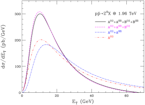
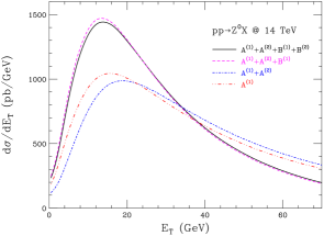
Figure 1: Resummed component of the transverse energy distribution in Z⁰ boson production at the Tevatron and LHC. The curves show the effects of the coefficients in the quark form factor: black, all coefficients; magenta omitting $B_{q}^{(2)}$; blue $A_{q}^{(1)}$ and $A_{q}^{(2)}$ only; red $A_{q}^{(1)}$ only.

Figure 1 shows the resummed component of the transverse energy distribution in Z⁰ boson production at the Tevatron ($p\bar{p}$ at $\sqrt{s}=1.96$ TeV) and LHC ($pp$ at $\sqrt{s}=14$ TeV). For all calculations, we use the MSTW 2008 NLO parton distributions [22]. The different curves show the effects of the subleading coefficients (31) in the quark form factor. We see that while $B_{q}^{(1)}$ has a large effect (the difference between the blue and magenta curves), the effects of the other subleading coefficients are quite small.

The peak of the resummed distribution lies at around $E_{T}\sim 10$ GeV at the Tevatron, rising to $\sim 14$ GeV at the LHC. This is comfortably below $M_{Z}$, justifying the resummation of logarithms of $E_{T}/M_{Z}$ in the peak region. However, at LHC energy the predicted distribution has a substantial tail at larger values of $E_{T}$, indicating that the higher-order terms generated by the resummation formula remain significant even when the logarithms are not large. In addition, the LHC prediction does not go to zero as it should at small $E_{T}$. However, this region is sensitive to the treatment of non-perturbative effects such as the behaviour of the strong coupling at low scales (we freeze its value below 1 GeV) and the upper limit in the integral over transverse time (we set $\tau_{\mbox{\scriptsize max}}=1/\Lambda$ where $\Lambda$ is the two-loop QCD scale parameter, set to 200 MeV here).

The resummed component for W^± boson production looks very similar, apart of course from the overall normalization, and therefore we do not show it here. Predictions with matching to fixed order will be presented in Section 4.

3.2 Higgs boson production

Figure 2 shows the resummed component of the transverse energy distribution in Higgs boson production at the Tevatron and LHC, for a Higgs mass of 115 GeV. The effects of subleading terms in the gluon form factor (2.3) are more marked than those of the quark form factor discussed above. The distribution peaks at large values of $E_{T}$, around 40 GeV at the Tevatron, rising to $\sim 50$ GeV at the LHC. This is due to the larger colour charge of the gluon. However, together with the large effects of subleading terms, it does make the reliability of the resummed predictions more questionable. Also in contrast to the vector boson case, the suppression at low and high $E_{T}$ is if anything too great, resulting in negative values below 16 GeV and above 120 GeV at Tevatron energy.

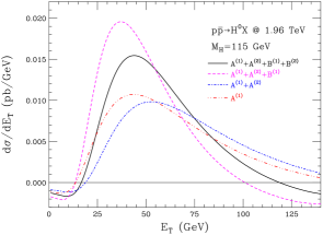
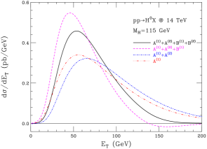
Figure 2: Resummed component of the transverse energy distribution in Higgs boson production at the Tevatron and LHC. The curves shows the effects of the coefficients in the gluon form factor: black, all coefficients; magenta omitting $B_{g}^{(2)}$; blue $A_{g}^{(1)}$ and $A_{g}^{(2)}$ only; red $A_{g}^{(1)}$ only.

4 Matching to fixed order

The resummed distributions presented above include only terms that are logarithmically enhanced at small $E_{T}$. To extend the predictions to larger $E_{T}$ we must match the resummation to fixed-order calculations. To avoid double counting of the resummed terms, the corresponding contribution must be subtracted from the fixed-order result.

We consider here only matching to first order in $\alpha_{\mathrm{S}}$. To this order the $E_{T}$ distribution for $E_{T}>0$ has the form

$$\frac{d\sigma}{dE_{T}}=\frac{1}{E_{T}}(A\ln E_{T}+B)+C(E_{T})$$ (42)

where $A$ and $B$ are constants (for a given process and collision energy) and the function $C(E_{T})$ is regular at $E_{T}=0$. The terms involving $A$ and $B$ are already included in the resummed prediction, and therefore we have only to add the regular function $C$ to it to obtain a prediction that is matched to the ${\cal O}(\alpha_{\mathrm{S}})$ result. This function is determined by fitting the ${\cal O}(\alpha_{\mathrm{S}})$ prediction for $E_{T}\,d\sigma/dE_{T}$ to a linear function of $\ln E_{T}$ at small $E_{T}$, extracting the coefficients $A$ and $B$, and then subtracting the enhanced terms in Eq. (42).

4.1 Vector boson production

Figure 3: Left: order-$\alpha_{\mathrm{S}}$ $E_{T}$ distribution in Z⁰ production at the Tevatron; solid, full prediction; dashed, fit to enhanced terms. Right: difference between full prediction and fit to enhanced terms.

Figure 4: Predicted $E_{T}$ distribution in Z⁰ production at the Tevatron and LHC. Solid: resummed prediction matched to ${\cal O}(\alpha_{\mathrm{S}})$. Dashed: resummed only. Dot-dashed: ${\cal O}(\alpha_{\mathrm{S}})$ only.

The above matching procedure is illustrated for Z⁰ production at the Tevatron in Fig. 3. The fit to the logarithmically enhanced terms gives excellent agreement with the order-$\alpha_{\mathrm{S}}$ result out to around 20 GeV, confirming the dominance of such terms throughout the region of the peak in Fig. 1. The remainder function $C(E_{T})$ vanishes at small $E_{T}$ and rises to around 10 pb/GeV, falling off slowly at large $E_{T}$. Consequently the matching correction to the resummed prediction is small and roughly constant throughout the region 40–100 GeV, as shown in Fig. 4.

As shown on the right in Fig. 4, the situation is similar at LHC energy: the matching correction is small, although in this case it is negative below about 40 GeV. The large tail at high $E_{T}$ and the bad behaviour at low $E_{T}$, due to uncompensated higher-order terms generated by resummation, are not much affected by matching to this order.

Figure 5: Predicted $E_{T}$ distribution in W⁺+W^- production at the Tevatron and LHC. Solid: resummed prediction matched to ${\cal O}(\alpha_{\mathrm{S}})$. Dashed: resummed only. Dot-dashed: ${\cal O}(\alpha_{\mathrm{S}})$ only.

The corresponding matched predictions for W^± boson production are shown in Fig. 5. As remarked earlier, the form of the resummed distribution is very similar to that for Z⁰ boson production, and again the matching correction is small.

4.2 Higgs boson production

Figure 6: Left: order-$\alpha_{\mathrm{S}}$ $E_{T}$ distribution in Higgs boson production at the Tevatron; solid, full prediction; dashed, fit to enhanced terms. Right: difference between full prediction and fit to enhanced terms.

Figure 7: Predicted $E_{T}$ distribution in Higgs boson production at the Tevatron and LHC. Solid: resummed prediction matched to ${\cal O}(\alpha_{\mathrm{S}})$. Dashed: resummed only. Dot-dashed: ${\cal O}(\alpha_{\mathrm{S}})$ only.

Adopting the same matching procedure for Higgs boson production, we find the results shown in Figs. 6 and 7. The form of the matching correction is similar to that for vector bosons, but its effect is rather different. The roughly constant, then slowly decreasing, correction in the region 20–100 GeV is not small compared to the resummed result and therefore it raises the whole distribution by a significant amount throughout this region. This has the beneficial effect of compensating the negative values at low and high $E_{T}$ at Tevatron energy. However, it further enhances the high-$E_{T}$ tail of the distribution at LHC energy. This, together with the relatively large correction in the peak region, casts further doubt on the reliability of the predictions in the case of Higgs production.

5 Monte Carlo comparisons

In this section we compare the resummed and matched distributions obtained above with the predictions of the parton shower Monte Carlo programs HERWIG [13] and Herwig++ [14].

Comparisons are performed first at the parton level, that is, after QCD showering from the incoming and outgoing partons of the hard subprocess. We say “incoming and outgoing” because both programs apply hard matrix element corrections: in addition to the Born process, order-$\alpha_{\mathrm{S}}$ real emission hard subprocesses are included in phase-space regions not covered by showering from the Born process.

After showering, the Monte Carlo programs apply a hadronization model to convert the partonic final state to a hadronic one. We show the effects of hadronization in the case of HERWIG only; those in Herwig++ are broadly similar since both programs use basically the same cluster hadronization model. The programs also model the underlying event, which arises from the interactions of spectator partons and makes a significant contribution to the hadronic transverse energy. In this case we show only the underlying event prediction of Herwig++, since the default model used in HERWIG has been found to give an unsatisfactory description of Tevatron data. For an improved simulation of the underlying event, HERWIG can be interfaced to the multiple interaction package JIMMY [23], which is similar to the model built into Herwig++.

5.1 Vector boson production

Figure 8 shows the comparisons for Z⁰ production at the Tevatron and LHC. The HERWIG predictions are renormalized by a factor of 1.3 to account for the increase in the cross section from LO to NLO. The Herwig++ results were not renormalized, because they were obtained using LO** parton distributions [24], which aim to reproduce the NLO cross section. We see that the parton-level Monte Carlo predictions of both programs agree fairly well with the matched resummed results above about 15 GeV, but Herwig++ generates a substantially higher number of events with low values of $E_{T}$. A similar pattern is evident in the results on W^± boson production, shown in Fig. 9. The effects of hadronization, shown by the difference between the blue and magenta histograms, are also similar for both vector bosons. They generate a significant shift in the distribution, of around 10 GeV at Tevatron energy and 20 GeV at LHC.

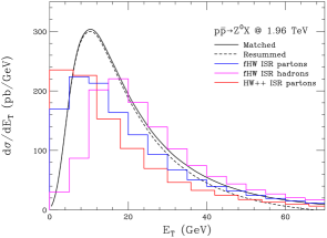
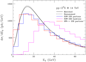
Figure 8: Predicted $E_{T}$ distribution in Z⁰ boson production at the Tevatron and LHC. Comparison of resummed and Monte Carlo results.

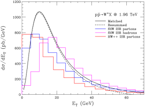
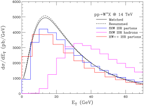
Figure 9: Predicted $E_{T}$ distribution in W⁺+W^- boson production at the Tevatron and LHC. Comparison of resummed and Monte Carlo results.

5.2 Higgs boson production

As may be seen from Fig. 10, the agreement between the resummed and parton-level Monte Carlo results is less good in the case of Higgs boson production than it was for vector bosons. Here we have renormalized the HERWIG predictions by a factor of 2 to allow for the larger NLO correction to the cross section. Then the Monte Carlo $E_{T}$ distributions agree quite well with each other but fall well below the matched resummed predictions. Fair agreement above about 40 GeV can be achieved by adjusting the normalization, but then the Monte Carlos predict more events at lower $E_{T}$. The effect of hadronization is similar to that in vector boson production, viz. a shift of about 10 GeV at the Tevatron rising to 20 GeV at the LHC, which actually brings the HERWIG distribution into somewhat better agreement with the resummed result.

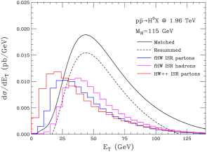
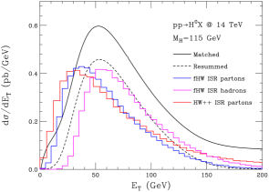
Figure 10: Predicted $E_{T}$ distribution in Higgs boson production at the Tevatron and LHC. Comparison of resummed and Monte Carlo results.

5.3 Modelling the underlying event

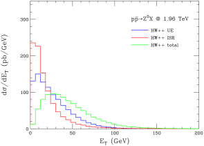
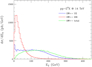
Figure 11: Predicted $E_{T}$ distribution in Z⁰ boson production at the Tevatron and LHC. Monte Carlo results including underlying event.

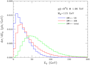
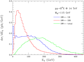
Figure 12: Predicted $E_{T}$ distribution in Higgs boson production at the Tevatron and LHC. Monte Carlo results including underlying event.

Figures 11 and 12 show the parton-level Herwig++ predictions for the $E_{T}$ distribution in Z⁰ and Higgs boson production, respectively, with the contributions from initial-state radiation (in red, already shown in Figs. 8 and 10 ), the underlying event (blue) and the combination of the two (green). The underlying event is modelled using multiple parton interactions; see ref. [14] for details. Clearly it has a very significant effect on the $E_{T}$ distribution. However, this effect is substantially independent of the hard subprocess, as may be seen from the comparison of different subprocesses in Fig. 13.

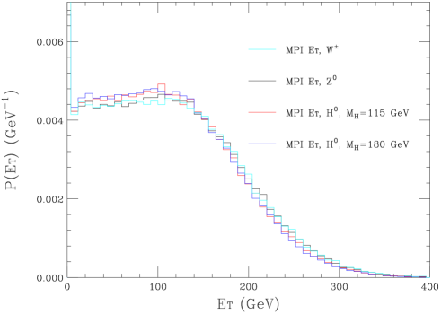
Figure 13: Comparison of $E_{T}$ distributions of the underlying event in different subprocesses at the LHC.

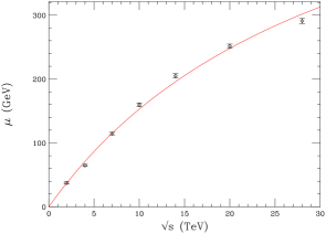
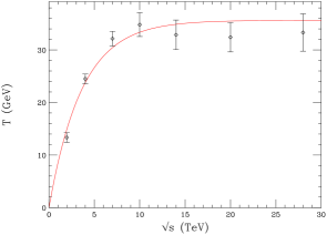
Figure 14: Fitted values of the parameters of the underlying event in Higgs production in $pp$ collisions at various energies.

We find that the probability distribution of the $E_{T}$ contribution of the underlying event in the Herwig++ Monte Carlo can be represented quite well by a Fermi distribution:

$$P(E_{T})=\frac{1}{\cal N}\frac{1}{\exp\left(\frac{E_{T}-\mu}{T}\right)+1}$$ (43)

where the normalization is

$${\cal N}=T\ln\left[\exp\left(\frac{\mu}{T}\right)+1\right]\;.$$ (44)

The dependence of the “chemical potential” $\mu$ and “temperature” $T$ on the hadronic collision energy is shown in Fig. 14. The red curves show fits to the energy dependence of the form

$$\mu=\frac{A\sqrt{s}}{1+B\sqrt{s}}\,,\quad T=q\left(1-{\rm e}^{-r\sqrt{s}}\right)$$ (45)

where the coefficients in the fits are $A=20(1)$, $B=0.030(4)$, $q=36(2)$, $r=0.28(3)$.

6 Conclusions

We have extended the resummation of the hadronic transverse energy $E_{T}$ in vector boson production to next-to-leading order (NLO) in the resummed exponent, parton distributions and coefficient functions, and also presented for the first time the corresponding predictions for Higgs boson production. We have matched the resummed results to the corresponding ${\cal O}(\alpha_{\mathrm{S}})$ predictions, by adding the contributions in that order which are not included in the resummation. In addition we have compared with parton shower Monte Carlo results and illustrated the effects of hadronization and the underlying event.

In the case of vector boson production, the resummation procedure appears stable and the parton-level results should be quite reliable. The leading-order mechanism of quark-antiquark annihilation typically generates a moderate amount of transverse energy in initial-state QCD radiation. Consequently the effects of subleading resummed terms and fixed-order matching are small and the peak of the $E_{T}$ distribution lies well below the boson mass scale, where resummation makes good sense. The comparisons with Monte Carlo programs reveal some discrepancies but these are at the level of disagreements between different programs; in this case the resummed predictions should be more reliable (at parton level) than existing Monte Carlos. The programs suggest that the non-perturbative effects of hadronization and the underlying event are substantial. These effects can however be modelled in a process-independent way. We have suggested a simple parametrization of the contribution of the underlying event.

The situation in Higgs boson production is not so good. The dominant mechanism of gluon fusion generates copious ISR and the effects of subleading terms and matching are large. The resummed $E_{T}$ distribution peaks at a value that is not parametrically smaller than the Higgs mass and the behaviour at low and high $E_{T}$ is unphysical before matching. The discrepancies between the matched resummed and Monte Carlo predictions are substantially greater than those between different programs, even allowing for uncertainties in the overall cross section. All this suggests that there are significant higher-order corrections that are not taken into account, either further subleading logarithms or unenhanced terms beyond NLO. It would be interesting (but very challenging) to attempt to extract such terms from the available NNLO calculations of Higgs production.

Appendix A Relation to transverse momentum resummation

Here we demonstrate the equivalence of transverse energy and transverse momentum resummation at order $\alpha_{\mathrm{S}}$. Expanding Eq. (7) to this order, using (11) and substituting into (5) and (6), we find terms involving the integrals

$${\cal I}_{p}(Q,E_{T})=\frac{1}{2\pi}\int_{-\infty}^{+\infty}d\tau\;{\rm e}^{-i\tau E_{T}}\ln^{p}\left(\frac{Q\tau}{i\tau_{0}}\right)$$ (46)

with $p=1,2$. At this order, evaluating the PDFs at the scale $i\tau_{0}/\tau$ leads to single-logarithmic terms of the same form when we use (13) to write

$$f_{a/h}(x,i\tau_{0}/\tau))=f_{a/h}(x,Q)-\frac{\alpha_{\mathrm{S}}}{\pi}\ln\left(\frac{Q\tau}{i\tau_{0}}\right)\sum_{b}\int_{x}^{1}\frac{dz}{z}P_{ab}(z)f_{b/h}(x/z,Q)\;.$$ (47)

The integral (46) may be evaluated from

$${\cal I}_{p}(Q,E_{T})=\frac{d^{p}}{du^{p}}{\cal I}(Q,E_{T};u)|_{u=0}$$ (48)

where

$${\cal I}(Q,E_{T};u)=\frac{1}{2\pi}\int_{-\infty}^{+\infty}d\tau\;{\rm e}^{-i\tau E_{T}}\;.\left(\frac{Q\tau}{i\tau_{0}}\right)^{u}$$ (49)

Writing $\tau=iz/E_{T}$, we have

$${\cal I}(Q,E_{T};u)=-\frac{i}{2\pi E_{T}}\left(\frac{Q}{E_{T}\tau_{0}}\right)^{u}\int_{-i\infty}^{+i\infty}dz\;z^{u}\,{\rm e}^{z}\;.$$ (50)

We can safely deform the integration contour around the branch cut along the negative real axis to obtain

$${\cal I}(Q,E_{T};u)=-\frac{1}{\pi E_{T}}\left(\frac{Q}{E_{T}\tau_{0}}\right)^{u}\sin(\pi u)\,\Gamma(1+u)\;,$$ (51)

which, recalling that $\ln\tau_{0}=-\gamma_{E}=\Gamma^{\prime}(1)$, gives

$${\cal I}_{1}(Q,E_{T})=-\frac{1}{E_{T}}\;,\quad{\cal I}_{2}(Q,E_{T})=-\frac{2}{E_{T}}\ln\left(\frac{Q}{E_{T}}\right)\;.$$ (52)

The resummed component of the transverse momentum ($q_{T}$) distribution takes the form

$$\left[\frac{d\sigma_{F}}{dQ^{2}\;dq_{T}}\right]_{{\rm res.}} = q_{T}\sum_{a,b}\int_{0}^{1}dx_{1}\int_{0}^{1}dx_{2}\int_{0}^{\infty}db\,b\,J_{0}(bq_{T})\;f_{a/h_{1}}(x_{1},b_{0}/b)\;f_{b/h_{2}}(x_{2},b_{0}/b)$$ (53)

$$\cdot \overline{W}_{ab}^{F}(x_{1}x_{2}s;Q,b)$$

where $b_{0}=2\exp(-\gamma_{E})$,

$$\overline{W}_{ab}^{F}(s;Q,b) = \sum_{c}\int_{0}^{1}dz_{1}\int_{0}^{1}dz_{2}\;C_{ca}(\alpha_{\mathrm{S}}(b_{0}/b),z_{1})\;C_{{\bar{c}}b}(\alpha_{\mathrm{S}}(b_{0}/b),z_{2})\;\delta(Q^{2}-z_{1}z_{2}s)$$ (54)

$$\cdot \sigma_{c{\bar{c}}}^{F}(Q,\alpha_{\mathrm{S}}(Q))\;\overline{S}_{c}(Q,b)$$

and

$$\overline{S}_{c}(Q,b)=\exp\left\{-2\int_{b_{0}/b}^{Q}\frac{dq}{q}\left[2A_{c}(\alpha_{\mathrm{S}}(q))\;\ln\frac{Q}{q}+B_{c}(\alpha_{\mathrm{S}}(q))\right]\right\}\;.$$ (55)

Expanding to order $\alpha_{\mathrm{S}}$, we find the same terms as in the $E_{T}$ resummation except that (46) is replaced by

$$\overline{\cal I}_{p}(Q,q_{T})=q_{T}\int_{0}^{\infty}db\,b\,J_{0}(bq_{T})\ln^{p}(Qb/b_{0})\;.$$ (56)

It therefore suffices to show that

$$\overline{\cal I}_{p}(Q,q_{T})={\cal I}_{p}(Q,E_{T}=q_{T})\;\;\;\mbox{for $p=1,2$.}$$ (57)

Now corresponding to (49) we have

$$\overline{\cal I}(Q,q_{T};u)=q_{T}\int_{0}^{\infty}db\,b\,J_{0}(bq_{T})\left(\frac{Qb}{b_{0}}\right)^{u}\;.$$ (58)

Using the result

$$\int_{0}^{\infty}dt\,t^{\mu-1}\,J_{0}(t)=\frac{2^{\mu}}{2\pi}\sin\left(\frac{\pi\mu}{2}\right)\Gamma^{2}\left(\frac{\mu}{2}\right)$$ (59)

gives

$$\overline{\cal I}(Q,q_{T};u)=-\frac{2}{\pi q_{T}}\left(\frac{2Q}{q_{T}b_{0}}\right)^{u}\sin\left(\frac{\pi u}{2}\right)\Gamma^{2}\left(1+\frac{u}{2}\right)$$ (60)

and hence

$$\overline{\cal I}_{1}(Q,q_{T})=-\frac{1}{q_{T}}\;,\quad\overline{\cal I}_{2}(Q,q_{T})=-\frac{2}{q_{T}}\ln\left(\frac{Q}{q_{T}}\right)\;,$$ (61)

in agreement with (52) and (57). Notice, however, that the higher ($p>2$) derivatives of ${\cal I}$ and $\overline{\cal I}$ differ, corresponding to the difference between $E_{T}$ and $q_{T}$ resummation beyond ${\cal O}(\alpha_{\mathrm{S}})$.

Appendix B Results for the LHC at 7 TeV

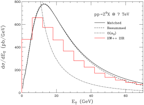
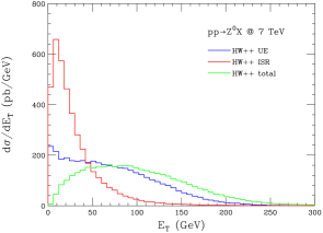
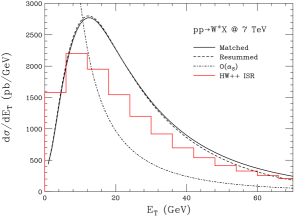
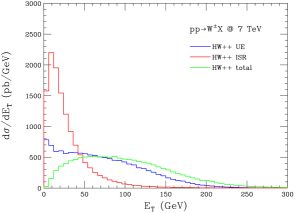
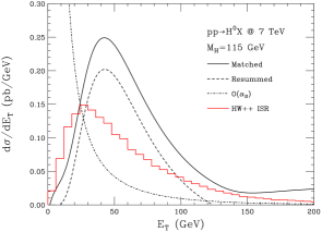
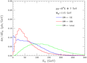
Figure 15: Predicted $E_{T}$ distributions in Z⁰, W⁺+W^- and Higgs boson production in $pp$ collisions at $\sqrt{s}=7$ TeV .

We show here results for the LHC operating at a centre-of-mass energy of 7 TeV, corresponding to those shown earlier for 14 TeV. Apart from the normalization, the predictions for the two energies are very similar, with only a slight downward shift in the position of the peak in the $E_{T}$ distribution at the lower energy.

References

• [1] G. Bozzi, S. Catani, D. de Florian and M. Grazzini, Nucl. Phys.  B 791 (2008) 1 [arXiv:0705.3887 [hep-ph]].
• [2] G. Bozzi, S. Catani, G. Ferrera, D. de Florian and M. Grazzini, Nucl. Phys.  B 815, 174 (2009) [arXiv:0812.2862 [hep-ph]].
• [3] S. Mantry and F. Petriello, arXiv:0911.4135.
• [4] Y. L. Dokshitzer, D. Diakonov and S. I. Troian, Phys. Rep.  58 (1980) 269.
• [5] G. Parisi and R. Petronzio, Nucl. Phys.  B154 (1979) 427.
• [6] G. Curci, M. Greco and Y. Srivastava, Nucl. Phys.  B159 (1979) 451.
• [7] A. Bassetto, M. Ciafaloni and G. Marchesini, Nucl. Phys.  B163 (1980) 477.
• [8] J. Kodaira and L. Trentadue, Phys. Lett.  B112 (1982) 66, Phys. Lett.  B123 (1983) 335.
• [9] J. C. Collins, D. E. Soper and G. Sterman, Nucl. Phys.  B 250 (1985) 199.
• [10] F. Halzen, A. D. Martin, D. M. Scott and M. P. Tuite, Z. Phys.  C 14 (1982) 351.
• [11] C. T. H. Davies and B. R. Webber, Z. Phys.  C 24 (1984) 133.
• [12] G. Altarelli, G. Martinelli and F. Rapuano, Z. Phys.  C 32 (1986) 369.
• [13] G. Corcella, I. G. Knowles, G. Marchesini, S. Moretti, K. Odagiri, P. Richardson, M. H. Seymour and B. R. Webber, JHEP 0101 (2001) 010 [arXiv:hep-ph/0011363]; arXiv:hep-ph/0210213. http://projects.hepforge.org/fherwig/
• [14] M. Bahr et al., Eur. Phys. J.  C 58 (2008) 639 [arXiv:0803.0883 [hep-ph]]; arXiv:0812.0529 [hep-ph]. http://projects.hepforge.org/herwig/
• [15] S. Catani, D. de Florian and M. Grazzini, Nucl. Phys.  B 596, 299 (2001) [arXiv:hep-ph/0008184].
• [16] C. T. Davies and W. J. Stirling, Nucl. Phys.  B244 (1984) 337.
• [17] C. Balazs, J. W. Qiu and C. P. Yuan, Phys. Lett.  B 355 (1995) 548 [arXiv:hep-ph/9505203].
• [18] D. de Florian and M. Grazzini, Phys. Rev. Lett.  85 (2000) 4678 [arXiv:hep-ph/0008152].
• [19] D. de Florian and M. Grazzini, Nucl. Phys.  B 616 (2001) 247 [arXiv:hep-ph/0108273].
• [20] S. Catani, E. D’Emilio and L. Trentadue, Phys. Lett.  B211 (1988) 335.
• [21] R. P. Kauffman, Phys. Rev.  D45 (1992) 1512.
• [22] A. D. Martin, W. J. Stirling, R. S. Thorne and G. Watt, Eur. Phys. J.  C 63 (2009) 189 [arXiv:0901.0002 [hep-ph]].
• [23] J. M. Butterworth, J. R. Forshaw and M. H. Seymour, Z. Phys.  C 72 (1996) 637 [arXiv:hep-ph/9601371]. http://projects.hepforge.org/jimmy/
• [24] A. Sherstnev and R. S. Thorne, Eur. Phys. J.  C 55 (2008) 553 [arXiv:0711.2473 [hep-ph]]; arXiv:0807.2132 [hep-ph].