On the Number of Higher Order Delaunay Triangulations

Abstract

Higher order Delaunay triangulations are a generalization of the Delaunay triangulation which provides a class of well-shaped triangulations, over which extra criteria can be optimized. A triangulation is order-$\color[rgb]{0.75,0.30,0.15}k$ Delaunay if the circumcircle of each triangle of the triangulation contains at most $\color[rgb]{0.75,0.30,0.15}k$ points. In this paper we study lower and upper bounds on the number of higher order Delaunay triangulations, as well as their expected number for randomly distributed points. We show that arbitrarily large point sets can have a single higher order Delaunay triangulation, even for large orders, whereas for first order Delaunay triangulations, the maximum number is $\color[rgb]{0.75,0.30,0.15}2^{n-3}$. Next we show that uniformly distributed points have an expected number of at least $\color[rgb]{0.75,0.30,0.15}2^{\rho_{1}n(1+o(1))}$ first order Delaunay triangulations, where $\color[rgb]{0.75,0.30,0.15}\rho_{1}$ is an analytically defined constant ($\color[rgb]{0.75,0.30,0.15}\rho_{1}\approx 0.525785$), and for $\color[rgb]{0.75,0.30,0.15}k>1$, the expected number of order-$\color[rgb]{0.75,0.30,0.15}k$ Delaunay triangulations (which are not order-$\color[rgb]{0.75,0.30,0.15}i$ for any $\color[rgb]{0.75,0.30,0.15}i<k$) is at least $\color[rgb]{0.75,0.30,0.15}2^{\rho_{k}n(1+o(1))}$, where $\color[rgb]{0.75,0.30,0.15}\rho_{k}$ can be calculated numerically.

1 Introduction

A triangulation is a decomposition into triangles. In this paper we are interested in triangulations of point sets in the Euclidean plane, where the input is a set of points in the plane, denoted $\color[rgb]{0.75,0.30,0.15}\cal P$, and a triangulation is defined as a subdivision of the convex hull of $\color[rgb]{0.75,0.30,0.15}\cal P$ into triangles whose vertices are the points in $\color[rgb]{0.75,0.30,0.15}\cal P$.

It is a well-known fact that $\color[rgb]{0.75,0.30,0.15}n$ points in the plane can have many different triangulations. For most application domains, the choice of the triangulation is important, because different triangulations can have different effects. For example, two important fields in which triangulations are frequently used are finite element methods and terrain modeling. In the first case, triangulations are used to subdivide a complex domain by creating a mesh of simple elements (triangles), over which a system of differential equations can be solved more easily. In the second case, the points in $\color[rgb]{0.75,0.30,0.15}\cal P$ represent points sampled from a terrain (thus each point has also an elevation), and the triangulation provides a bivariate interpolating surface, providing an elevation model of the terrain. In both cases, the shapes of the triangles can have serious consequences on the result. For mesh generation for finite element methods, the aspect ratio of the triangles is particularly important, since elements of large aspect ratio can lead to poorly-conditioned systems. Similarly, long and skinny triangles are generally not appropriate for surface interpolation because they can lead to interpolation from points that are too far apart.

In most applications, the need for well-shaped triangulations is usually addressed by using the Delaunay triangulation. The Delaunay triangulation of a point set $\color[rgb]{0.75,0.30,0.15}\cal P$ is defined as a triangulation where the vertices are the points in $\color[rgb]{0.75,0.30,0.15}\cal P$ and the circumcircle of each triangle (that is, the circle defined by the three vertices of each triangle) contains no other point from $\color[rgb]{0.75,0.30,0.15}\cal P$. The Delaunay triangulation has many known properties that make it the most widely-used triangulation. In particular, there are several efficient and relatively simple algorithms to compute it, and its triangles are considered well-shaped. This is because it maximizes the minimum angle among all triangle angles, which implies that its angles are—in a sense—as large as possible. Moreover, when the points are in general position (that is, when no four points are cocircular and no three points are collinear) it is uniquely defined. However, this last property can become an important limitation if the Delaunay triangulation is suboptimal with respect to other criteria, independent of the shape of its triangles, as it is often the case in applications.

To overcome this limitation, Gudmundsson et al. proposed higher order Delaunay triangulations [10]. They are a natural generalization of the Delaunay triangulation that provides well-shaped triangles, but at the same time, flexibility to optimize some extra criterion. They are defined by allowing up to $\color[rgb]{0.75,0.30,0.15}k$ points inside the circumcircles of the triangles (see Figure 1). For $\color[rgb]{0.75,0.30,0.15}k=0$, each point set in general position has only one higher order Delaunay triangulation, equal to the Delaunay triangulation. As the parameter $\color[rgb]{0.75,0.30,0.15}k$ is increased, more points inside the circumcircles imply a reduction of the shape quality of the triangles, but also an increase in the number of triangulations that are considered. This last aspect makes the optimization of extra criteria possible, thus providing triangulations that are a compromise between well-shaped triangles and optimality with respect to other criteria.

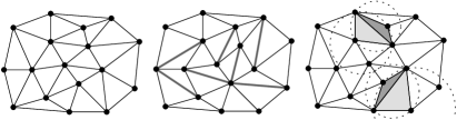
Figure 1: Left: A Delaunay triangulation ($\color[rgb]{0.75,0.30,0.15}k=0$). Center: an order-$\color[rgb]{0.75,0.30,0.15}1$ triangulation (with useful-1, non-Delaunay, edges in gray). Right: an order-$\color[rgb]{0.75,0.30,0.15}2$ triangulation, with order-1 triangles in light gray and order-2 triangles in medium gray.

Therefore the importance of higher order Delaunay triangulations lies in multi-criteria triangulations. Their major contribution is providing a way to optimize over a—hopefully large—class of well-shaped triangulations.

A particularly important subclass of higher order Delaunay triangulations are the first order Delaunay triangulations, that is, when $\color[rgb]{0.75,0.30,0.15}k=1$. It has been observed that already for $\color[rgb]{0.75,0.30,0.15}k=1$, a point set with $\color[rgb]{0.75,0.30,0.15}n$ points can have an exponential number of different triangulations [16]. This, together with the fact that for $\color[rgb]{0.75,0.30,0.15}k=1$ the shape of the triangles is as close as possible to the shape of the Delaunay triangles (while allowing more than one triangulation to choose from), make first order Delaunay triangulations especially interesting. In fact, first order Delaunay triangulations have been shown to have a special structure that facilitates the optimization of many criteria [10]. For example, it has been shown that many criteria related to measures of single triangles, as well as some other relevant parameters like the number of local minima, can be optimized in $\color[rgb]{0.75,0.30,0.15}O(n\log n)$ time for $\color[rgb]{0.75,0.30,0.15}k=1$. In a recent paper [17], Van Kreveld et al. studied several types of more complex optimization problems, constrained to first order Delaunay triangulations. They showed that many other criteria can be also optimized efficiently for $\color[rgb]{0.75,0.30,0.15}k=1$, making first order Delaunay triangulations even more appealing for practical use.

For larger values of $\color[rgb]{0.75,0.30,0.15}k$, fewer results are known. The special structure of first order Delaunay triangulations is not present anymore, which complicates exact optimization algorithms. Several heuristics and experimental results have been presented for optimization problems related to terrain modeling, showing that very small values of $\color[rgb]{0.75,0.30,0.15}k$ ($\color[rgb]{0.75,0.30,0.15}k=1,\ldots,8$) are enough to achieve important improvements for several terrain criteria [4, 5, 8].

However, despite the importance given to finding algorithms to optimize over higher order Delaunay triangulations, it has never been studied before how many higher order Delaunay triangulations there can be in the first place. In other words, it is not known what the minimum and maximum number of different triangulations are, as functions of $\color[rgb]{0.75,0.30,0.15}k$ and $\color[rgb]{0.75,0.30,0.15}n$, not even for the simpler (but—in practice—most important) case of first order Delaunay triangulations.

The problem of determining bounds on the number of higher order Delaunay triangulations is of both theoretical and practical interest.

From a theoretical point of view, determining how many triangulations a point set has is one of the most intriguing problems in combinatorial geometry, and has received a lot of attention (e.g. [2, 15, 14]). Higher order Delaunay triangulations are a natural and simple generalization of the Delaunay triangulation, hence the impact of such generalization on the number of triangulations is worth studying.

From a more practical point of view, knowing the number of triangulations for a given $\color[rgb]{0.75,0.30,0.15}k$ gives an idea of how large the solution space is when optimizing over this class of well-shaped triangulations. Ideally, one expects to have many different triangulations to choose from, in order to find one that is good with respect to other criteria.

Up to now, only trivial bounds were known: every point set has at least one order-$\color[rgb]{0.75,0.30,0.15}k$ Delaunay triangulation, for any $\color[rgb]{0.75,0.30,0.15}k$ (equal to the Delaunay triangulation), and there are point sets of size $\color[rgb]{0.75,0.30,0.15}n$ that have $\color[rgb]{0.75,0.30,0.15}2^{\Theta(n)}$ triangulations, already for $\color[rgb]{0.75,0.30,0.15}k=1$. In this paper we present the first non-trivial bounds on the number of higher order Delaunay triangulations. Given the practical motivation mentioned above, we are mostly interested in results that have practical implications for the use of higher order Delaunay triangulations. Thus low values of $\color[rgb]{0.75,0.30,0.15}k$ are our main concern. Our ultimate goal—achieved partially in this paper—is to determine to what extent the class of higher order Delaunay triangulations (for small values of $\color[rgb]{0.75,0.30,0.15}k$, which has the best triangle-shape properties), also provides a large number of triangulations to choose from.

Results

We study lower and upper bounds on the number of higher order Delaunay triangulations, as well as the expected number of order-$\color[rgb]{0.75,0.30,0.15}k$ Delaunay triangulations for uniformly distributed points. Let $\color[rgb]{0.75,0.30,0.15}T_{k}(n)$ denote the maximum number of order-$\color[rgb]{0.75,0.30,0.15}k$ Delaunay triangulations that a set with $\color[rgb]{0.75,0.30,0.15}n$ points can have, and let $\color[rgb]{0.75,0.30,0.15}t_{k}(n)$ denote the minimum number of order-$\color[rgb]{0.75,0.30,0.15}k$ Delaunay triangulations that a set with $\color[rgb]{0.75,0.30,0.15}n$ points can have. First we show that the lower bound $\color[rgb]{0.75,0.30,0.15}t_{k}(n)\geq 1$ is tight. In other words, there are arbitrarily large point sets that have a single higher order Delaunay triangulation, even for large values of $\color[rgb]{0.75,0.30,0.15}k$. Next we show that, for first order Delaunay triangulations, $\color[rgb]{0.75,0.30,0.15}T_{1}(n)=2^{n-3}$. Since these extreme cases do not describe an average situation when higher order Delaunay triangulations are used, we then study the number of higher order Delaunay triangulations for a uniformly distributed point set. Let $\color[rgb]{0.75,0.30,0.15}R_{k}$ denote the number of order-$\color[rgb]{0.75,0.30,0.15}k$ (and not order-$\color[rgb]{0.75,0.30,0.15}i,$ for any $\color[rgb]{0.75,0.30,0.15}i<k$) Delaunay triangulations of a uniformly distributed point set of size $\color[rgb]{0.75,0.30,0.15}n$. We show that $\color[rgb]{0.75,0.30,0.15}{\mathbb{E}}[R_{1}]\geq 2^{\rho_{1}n(1+o(1))}$, where $\color[rgb]{0.75,0.30,0.15}\rho_{1}$ is an analytically defined constant ($\color[rgb]{0.75,0.30,0.15}\rho_{1}\approx 0.525785$). We also prove that, for constant values of $\color[rgb]{0.75,0.30,0.15}k,$ $\color[rgb]{0.75,0.30,0.15}{\mathbb{E}}[R_{k}]\geq 2^{\rho_{k}n(1+o(1))}$, where $\color[rgb]{0.75,0.30,0.15}\rho_{k}$ can be calculated numerically (asymptotics are with respect to $\color[rgb]{0.75,0.30,0.15}n$). The result has interesting practical consequences, since it implies that it is reasonable to expect an exponential number of higher order Delaunay triangulations for any $\color[rgb]{0.75,0.30,0.15}k\geq 1$.

Related work

As mentioned earlier, there is no previous work on counting higher order Delaunay triangulations. A related concept, the higher order Delaunay graph, has been studied by Abellanas et al. [1]. The order-$\color[rgb]{0.75,0.30,0.15}k$ Delaunay graph of a set of points $\color[rgb]{0.75,0.30,0.15}\cal P$ is a graph with vertex set $\color[rgb]{0.75,0.30,0.15}\cal P$ and an edge between two points $\color[rgb]{0.75,0.30,0.15}p,q$ when there is a circle through $\color[rgb]{0.75,0.30,0.15}p$ and $\color[rgb]{0.75,0.30,0.15}q$ containing at most $\color[rgb]{0.75,0.30,0.15}k$ other points from $\color[rgb]{0.75,0.30,0.15}\cal P$. Abellanas et al. presented upper and lower bounds on the number of edges of this graph. However, since a triangulation that is a subset of the order-$\color[rgb]{0.75,0.30,0.15}k$ Delaunay graph does not need to be an order-$\color[rgb]{0.75,0.30,0.15}k$ Delaunay triangulation, it is difficult to derive good bounds for higher order Delaunay triangulations based on them.

There is an ample body of literature on the more general problem of counting all triangulations. Lower and upper bounds on the number of triangulations that $\color[rgb]{0.75,0.30,0.15}n$ points can have have been improved many times over the years, with the current best ones establishing that there are point sets that have $\color[rgb]{0.75,0.30,0.15}\Omega(8.48^{n})$ [2] triangulations, whereas no point set can have more than $\color[rgb]{0.75,0.30,0.15}O(43^{n})$ [15].

In relation to our expected case analysis of the number of higher order Delaunay triangulations, it is worth mentioning that many properties of the Delaunay triangulation—and related proximity graphs—of random points have been studied. The expected behavior of properties of the Delaunay triangulation that have been considered include the average and maximum edge length [12, 3], the minimum and maximum angles [3], and its expected weight [6]. Expected properties of other proximity graphs, such as the Gabriel graph and some relatives, are investigated in [9, 7, 11].

Outline

This paper is structured as follows. The next section presents some previous results related to higher order Delaunay triangulations, needed for the following sections. In Section 3 we give lower and upper bounds for the number of higher order Delaunay triangulations. Section 4 deals with the expected number of higher order Delaunay triangulations. Finally, some concluding remarks are made in Section 5.

2 Higher order Delaunay triangulations

We begin by introducing higher order Delaunay triangulations more formally, and presenting a few properties that will be used throughout the paper. From now on, we assume that point sets are in general position.

Definition 1

(from [10]) A triangle $\color[rgb]{0.75,0.30,0.15}\triangle uvw$ in a point set $\color[rgb]{0.75,0.30,0.15}\cal P$ is order-$\color[rgb]{0.75,0.30,0.15}k$ Delaunay if its circumcircle $\color[rgb]{0.75,0.30,0.15}C(u,v,w)$ contains at most $\color[rgb]{0.75,0.30,0.15}k$ points of $\color[rgb]{0.75,0.30,0.15}\cal P$. A triangulation of $\color[rgb]{0.75,0.30,0.15}\cal P$ is order-$\color[rgb]{0.75,0.30,0.15}k$ Delaunay if every triangle of the triangulation is order-$\color[rgb]{0.75,0.30,0.15}k$.

Note that if a triangle or triangulation is order-$\color[rgb]{0.75,0.30,0.15}k$, it is also order-$\color[rgb]{0.75,0.30,0.15}k^{\prime}$ for any $\color[rgb]{0.75,0.30,0.15}k^{\prime}>k$. A simple corollary of this is that, for any point set and any $\color[rgb]{0.75,0.30,0.15}k\geq 0$, the Delaunay triangulation is an order-$\color[rgb]{0.75,0.30,0.15}k$ Delaunay triangulation.

Definition 2

(from [10]) An edge $\color[rgb]{0.75,0.30,0.15}\overline{uv}$ is an order-$\color[rgb]{0.75,0.30,0.15}k$ Delaunay edge if there exists a circle through $\color[rgb]{0.75,0.30,0.15}u$ and $\color[rgb]{0.75,0.30,0.15}v$ that has at most $\color[rgb]{0.75,0.30,0.15}k$ points of $\color[rgb]{0.75,0.30,0.15}\cal P$ inside. An edge $\color[rgb]{0.75,0.30,0.15}\overline{uv}$ is a useful order-$\color[rgb]{0.75,0.30,0.15}k$ Delaunay edge (or simply useful-$\color[rgb]{0.75,0.30,0.15}k$ edge) if there is an order-$\color[rgb]{0.75,0.30,0.15}k$ Delaunay triangulation that contains $\color[rgb]{0.75,0.30,0.15}\overline{uv}$.

The useful order of an edge can be checked using the following lemma, illustrated in Figure 2.

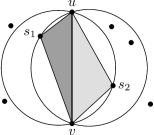
Figure 2: The useful order of edge $\color[rgb]{0.75,0.30,0.15}\overline{uv}$ is determined by the lowest order of triangles $\color[rgb]{0.75,0.30,0.15}\triangle uvs_{1}$ and $\color[rgb]{0.75,0.30,0.15}\triangle uvs_{2}$. In the example, the (lowest) useful order of $\color[rgb]{0.75,0.30,0.15}\overline{uv}$ is $\color[rgb]{0.75,0.30,0.15}\max\{3,1\}=3$.

Lemma 1

(from [10]) Let $\color[rgb]{0.75,0.30,0.15}\overline{uv}$ be an order-$\color[rgb]{0.75,0.30,0.15}k$ Delaunay edge, let $\color[rgb]{0.75,0.30,0.15}s_{1}$ be the point to the left of $\color[rgb]{0.75,0.30,0.15}\overrightarrow{vu}$, such that the circle $\color[rgb]{0.75,0.30,0.15}C(u,v,s_{1})$ contains no points to the left of $\color[rgb]{0.75,0.30,0.15}\overrightarrow{vu}$. Let $\color[rgb]{0.75,0.30,0.15}s_{2}$ be defined similarly but to the right of $\color[rgb]{0.75,0.30,0.15}\overrightarrow{vu}$. Edge $\color[rgb]{0.75,0.30,0.15}\overline{uv}$ is useful-$\color[rgb]{0.75,0.30,0.15}k$ if and only if $\color[rgb]{0.75,0.30,0.15}\triangle{uvs_{1}}$ and $\color[rgb]{0.75,0.30,0.15}\triangle{uvs_{2}}$ are order-$\color[rgb]{0.75,0.30,0.15}k$ Delaunay triangles.

The concept of a fixed edge is important in order to study the structure of higher order Delaunay triangulations.

Definition 3

Let $\color[rgb]{0.75,0.30,0.15}\cal P$ be a point set and $\color[rgb]{0.75,0.30,0.15}T$ its Delaunay triangulation. An edge of $\color[rgb]{0.75,0.30,0.15}T$ is $\color[rgb]{0.75,0.30,0.15}k$-fixed if it is present in every order-$\color[rgb]{0.75,0.30,0.15}k$ Delaunay triangulation of $\color[rgb]{0.75,0.30,0.15}\cal P$.

Some simple observations derived from this are that the convex hull edges are always $\color[rgb]{0.75,0.30,0.15}k$-fixed, for any $\color[rgb]{0.75,0.30,0.15}k$, and that all the Delaunay edges are $\color[rgb]{0.75,0.30,0.15}0$-fixed.

First order Delaunay triangulations have a special structure. If we take all edges that are 1-fixed, then the resulting subdivision has only triangles and convex quadrilaterals (and an unbounded face). In the convex quadrilaterals, both diagonals are possible to obtain a first order Delaunay triangulation (see Figure 1, center). We say that both diagonals are flippable, and similarly we call the quadrilateral flippable. More formally, based on results in [10], we can make the following observation.

Observation 1

Let $\color[rgb]{0.75,0.30,0.15}e$ be a useful order-1 Delaunay edge in an order-1 Delaunay triangulation, such that $\color[rgb]{0.75,0.30,0.15}e$ is not a Delaunay edge. Then flipping $\color[rgb]{0.75,0.30,0.15}e$ results in a Delaunay edge. Moreover, the four edges (different from $\color[rgb]{0.75,0.30,0.15}e$) that bound the two triangles adjacent to $\color[rgb]{0.75,0.30,0.15}e$ are 1-fixed edges.

An implication of this special structure is that instead of counting triangulations, we can count flippable quadrilaterals or, equivalently, useful-1 edges that are not Delaunay.

Corollary 1

Let $\color[rgb]{0.75,0.30,0.15}\cal P$ be a point set. If $\color[rgb]{0.75,0.30,0.15}\cal P$ has $\color[rgb]{0.75,0.30,0.15}q$ flippable quadrilaterals, then $\color[rgb]{0.75,0.30,0.15}\cal P$ has exactly $\color[rgb]{0.75,0.30,0.15}2^{q}$ order-1 Delaunay triangulations.

For $\color[rgb]{0.75,0.30,0.15}k>1$, the structure is not so simple anymore and it seems difficult to provide an exact expression for the number of order-$\color[rgb]{0.75,0.30,0.15}k$ Delaunay triangulations in terms of the number of useful-$\color[rgb]{0.75,0.30,0.15}k$ edges. However, we can derive a lower bound by combining a number of known results, as follows. First we need some extra definitions and previous results:

Definition 4

(from [10]) The hull of an order-$\color[rgb]{0.75,0.30,0.15}k$ Delaunay edge $\color[rgb]{0.75,0.30,0.15}\overline{uv}$ ($\color[rgb]{0.75,0.30,0.15}k\geq 1$) is the closure of the union of all Delaunay triangles whose interior intersects $\color[rgb]{0.75,0.30,0.15}\overline{uv}.$

Lemma 2

(from [10]) The hull of an order-$\color[rgb]{0.75,0.30,0.15}k$ Delaunay edge ($\color[rgb]{0.75,0.30,0.15}k\geq 1$) is a simple polygon consisting of at most $\color[rgb]{0.75,0.30,0.15}2k+2$ vertices.

Lemma 3

(from [10]) Let $\color[rgb]{0.75,0.30,0.15}\overline{uv}$ be a useful-$\color[rgb]{0.75,0.30,0.15}k$ edge (and not useful-$\color[rgb]{0.75,0.30,0.15}i$ for any $\color[rgb]{0.75,0.30,0.15}i<k$), with $\color[rgb]{0.75,0.30,0.15}k\geq 1.$ There exists an order-$\color[rgb]{0.75,0.30,0.15}k$ (and not order-$\color[rgb]{0.75,0.30,0.15}i$ for any $\color[rgb]{0.75,0.30,0.15}i<k$) Delaunay triangulation of the hull of $\color[rgb]{0.75,0.30,0.15}\overline{uv}$ that contains $\color[rgb]{0.75,0.30,0.15}\overline{uv}.$

Lemma 4

Let $\color[rgb]{0.75,0.30,0.15}\overline{uv}$ be an order-$\color[rgb]{0.75,0.30,0.15}0$ edge. The number of useful-$\color[rgb]{0.75,0.30,0.15}k$ edges ($\color[rgb]{0.75,0.30,0.15}k\geq 1$) that intersect $\color[rgb]{0.75,0.30,0.15}\overline{uv}$ is at most $\color[rgb]{0.75,0.30,0.15}(2k+1)^{2}.$

Proof 2.1.

It follows directly from the proof of Lemma 8 in [10].

We have now the necessary tools to prove the following lower bound on the number of order-$\color[rgb]{0.75,0.30,0.15}k$ triangulations, expressed as a function of the number of useful-$\color[rgb]{0.75,0.30,0.15}k$ edges.

Lemma 2.2.

Let $\color[rgb]{0.75,0.30,0.15}\cal P$ be a point set and let $\color[rgb]{0.75,0.30,0.15}e_{k},$ for $\color[rgb]{0.75,0.30,0.15}k>1,$ be the number of useful-$\color[rgb]{0.75,0.30,0.15}k$ edges (which are not useful-$\color[rgb]{0.75,0.30,0.15}i$ for any $\color[rgb]{0.75,0.30,0.15}i<k$) of $\color[rgb]{0.75,0.30,0.15}\cal P.$ Then $\color[rgb]{0.75,0.30,0.15}\cal P$ has at least $\color[rgb]{0.75,0.30,0.15}2^{e_{k}/C_{k}}-1$ order-$\color[rgb]{0.75,0.30,0.15}k$ (and not order-$\color[rgb]{0.75,0.30,0.15}i,$ for any $\color[rgb]{0.75,0.30,0.15}i<k$) Delaunay triangulations, where $\color[rgb]{0.75,0.30,0.15}C_{k}=(4k+1)(2k+1)^{2}+1.$

Proof 2.3.

Let $\color[rgb]{0.75,0.30,0.15}E_{k}$ denote the set of useful-$\color[rgb]{0.75,0.30,0.15}k$ edges (which are not useful-$\color[rgb]{0.75,0.30,0.15}i$ for any $\color[rgb]{0.75,0.30,0.15}i<k$) of $\color[rgb]{0.75,0.30,0.15}\cal P$ and let $\color[rgb]{0.75,0.30,0.15}e_{k}$ denote the cardinal number of $\color[rgb]{0.75,0.30,0.15}E_{k}.$ We select a subset $\color[rgb]{0.75,0.30,0.15}E^{\prime}_{k}$ of the edges of $\color[rgb]{0.75,0.30,0.15}E_{k}$ in the following way: We pick an edge $\color[rgb]{0.75,0.30,0.15}e$ of $\color[rgb]{0.75,0.30,0.15}E_{k},$ we remove all the edges in $\color[rgb]{0.75,0.30,0.15}E_{k}$ whose hull intersects the hull of $\color[rgb]{0.75,0.30,0.15}e$ in at least one Delaunay triangle, and we repeat until $\color[rgb]{0.75,0.30,0.15}E_{k}$ does not contain any edge.

Let $\color[rgb]{0.75,0.30,0.15}e^{\prime}$ be an edge in $\color[rgb]{0.75,0.30,0.15}E^{\prime}_{k}$ and $\color[rgb]{0.75,0.30,0.15}e$ be an edge in $\color[rgb]{0.75,0.30,0.15}E_{k}$ whose hull intersects the hull of $\color[rgb]{0.75,0.30,0.15}e^{\prime}$ in at least one Delaunay triangle $\color[rgb]{0.75,0.30,0.15}T.$ Then $\color[rgb]{0.75,0.30,0.15}e$ intersects at least one edge of $\color[rgb]{0.75,0.30,0.15}T.$ By Lemma 2, all Delaunay triangles included in the hull of $\color[rgb]{0.75,0.30,0.15}e^{\prime}$ contain at most $\color[rgb]{0.75,0.30,0.15}4k+1$ edges. By Lemma 4, each of them intersects at most $\color[rgb]{0.75,0.30,0.15}(2k+1)^{2}$ useful-$\color[rgb]{0.75,0.30,0.15}k$ edges. Hence if $\color[rgb]{0.75,0.30,0.15}e^{\prime}$ is selected, at most $\color[rgb]{0.75,0.30,0.15}(4k+1)(2k+1)^{2}$ edges in $\color[rgb]{0.75,0.30,0.15}E_{k}$ are removed. Therefore $\color[rgb]{0.75,0.30,0.15}E^{\prime}_{k}$ contains at least $\color[rgb]{0.75,0.30,0.15}e_{k}/((4k+1)(2k+1)^{2}+1)$ edges.

Each non-empty subset of $\color[rgb]{0.75,0.30,0.15}E^{\prime}_{k}$ gives rise to a different order-$\color[rgb]{0.75,0.30,0.15}k$ (and not order-$\color[rgb]{0.75,0.30,0.15}i,$ for any $\color[rgb]{0.75,0.30,0.15}i<k$) Delaunay triangulation proceeding as follows: If an edge $\color[rgb]{0.75,0.30,0.15}e$ is in the subset, we triangulate the hull of $\color[rgb]{0.75,0.30,0.15}e$ as in Lemma 3, that is, we use an order-$\color[rgb]{0.75,0.30,0.15}k$ (and not order-$\color[rgb]{0.75,0.30,0.15}i,$ for any $\color[rgb]{0.75,0.30,0.15}i<k$) Delaunay triangulation containing $\color[rgb]{0.75,0.30,0.15}e.$ If an edge $\color[rgb]{0.75,0.30,0.15}e$ is not in the subset $\color[rgb]{0.75,0.30,0.15}E^{\prime}_{k}$, we triangulate the hull of $\color[rgb]{0.75,0.30,0.15}e$ using the Delaunay triangles crossed by $\color[rgb]{0.75,0.30,0.15}e.$ Finally, we complete the triangulation by adding Delaunay triangles in the regions that have not been triangulated (that is, computing a constrained Delaunay triangulation). This construction is consistent because the hulls of the edges in $\color[rgb]{0.75,0.30,0.15}E^{\prime}_{k}$ can only intersect in points and boundary edges, and because the boundary edges of the hulls belong to the Delaunay triangulation.

3 Lower and upper bounds

In this section we derive upper and lower bounds on the number of first order Delaunay triangulations. As mentioned in the introduction, due to the practical motivation of this work, we are mostly interested in lower bounds. However, for completeness and because the theoretical question is also interesting, this section also includes a result on upper bounds.

The main question that we address in this section is: what is the minimum number of higher order Delaunay triangulations that $\color[rgb]{0.75,0.30,0.15}n$ points can have? Are there arbitrarily large point sets that have only $\color[rgb]{0.75,0.30,0.15}O(1)$ higher order Delaunay triangulations? To our surprise, the answer to the second question is affirmative.

The lemma below presents a construction that has only one higher order Delaunay triangulation, regardless of the value of $\color[rgb]{0.75,0.30,0.15}k$, for any $\color[rgb]{0.75,0.30,0.15}k\leq\left\lfloor n/3\right\rfloor-1$. Note that this implies that for any value of $\color[rgb]{0.75,0.30,0.15}k$ of practical interest, there are point sets that have no other order-$\color[rgb]{0.75,0.30,0.15}k$ Delaunay triangulation than the Delaunay triangulation.

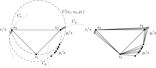
Figure 3: Construction of a point set (left) whose only order-$\color[rgb]{0.75,0.30,0.15}k$ Delaunay triangulation is the Delaunay triangulation (right).

Lemma 3.4.

Given any $\color[rgb]{0.75,0.30,0.15}n\geq 6$ and any $\color[rgb]{0.75,0.30,0.15}k$ such that $\color[rgb]{0.75,0.30,0.15}k\leq\left\lfloor n/3\right\rfloor-1$, there are point sets with $\color[rgb]{0.75,0.30,0.15}n$ points in general position that have only one order-$\color[rgb]{0.75,0.30,0.15}k$ Delaunay triangulation.

Proof 3.5.

We give a construction with $\color[rgb]{0.75,0.30,0.15}n$ points that can be shown to have only one order-$\color[rgb]{0.75,0.30,0.15}k$ Delaunay triangulation, for any value of $\color[rgb]{0.75,0.30,0.15}k\leq\left\lfloor n/3\right\rfloor-1$. The construction is illustrated in Figure 3.

To simplify the explanation, in the following we assume that $\color[rgb]{0.75,0.30,0.15}n$ is a multiple of 3. Since any order-$\color[rgb]{0.75,0.30,0.15}i$ Delaunay triangulation is also order-$\color[rgb]{0.75,0.30,0.15}k$ for all $\color[rgb]{0.75,0.30,0.15}k\geq i$, for the proof it is enough to use $\color[rgb]{0.75,0.30,0.15}k=n/3-1$.

We start with a triangle $\color[rgb]{0.75,0.30,0.15}\triangle s_{1}s_{2}s_{3}$. Then we add three groups of points, which we will denote with letters $\color[rgb]{0.75,0.30,0.15}p$, $\color[rgb]{0.75,0.30,0.15}q$, and $\color[rgb]{0.75,0.30,0.15}r$. The points in the first group are denoted $\color[rgb]{0.75,0.30,0.15}p_{1}\dots p_{m}$, where $\color[rgb]{0.75,0.30,0.15}m=n/3$. These points are initially placed on a circle $\color[rgb]{0.75,0.30,0.15}C_{p}$ that goes through $\color[rgb]{0.75,0.30,0.15}s_{3}$, as shown in the figure; they are sorted from top to bottom. The second group comprises $\color[rgb]{0.75,0.30,0.15}k$ points $\color[rgb]{0.75,0.30,0.15}q_{1}\dots q_{k}$, placed very close to each other on a circle $\color[rgb]{0.75,0.30,0.15}C_{q}$ through $\color[rgb]{0.75,0.30,0.15}s_{3}$, as shown in the figure. In addition, we must also make sure that the points $\color[rgb]{0.75,0.30,0.15}q_{1}\dots q_{k}$ are close enough to $\color[rgb]{0.75,0.30,0.15}s_{3}$ in order to be contained inside $\color[rgb]{0.75,0.30,0.15}C(s_{1},s_{2},p_{1})$. Finally, the points in the third group, $\color[rgb]{0.75,0.30,0.15}r_{1}\dots r_{k-1}$, are placed very close to each other on a third circle $\color[rgb]{0.75,0.30,0.15}C_{r}$, which goes through $\color[rgb]{0.75,0.30,0.15}s_{2}$. The important properties of these circles are: (i) $\color[rgb]{0.75,0.30,0.15}C_{p}$ contains $\color[rgb]{0.75,0.30,0.15}s_{2}$ and all the points $\color[rgb]{0.75,0.30,0.15}r_{i}$, (ii) $\color[rgb]{0.75,0.30,0.15}C_{r}$ and $\color[rgb]{0.75,0.30,0.15}C_{q}$ contain all the points of the type $\color[rgb]{0.75,0.30,0.15}p_{i}$, and (iii) $\color[rgb]{0.75,0.30,0.15}C(s_{1},s_{2},p_{1})$ contains $\color[rgb]{0.75,0.30,0.15}s_{3}$ and all points of type $\color[rgb]{0.75,0.30,0.15}q_{i}$.

Clearly, the point set as constructed is degenerate, but this can be easily solved by applying a slight perturbation to each point, without affecting the properties just mentioned. Moreover, the perturbation can be made such that the Delaunay triangulation of the point set looks like the one in the right of Figure 3.

We now argue that all the edges in the Delaunay triangulation are $\color[rgb]{0.75,0.30,0.15}k$-fixed, by considering the different types of edges that, potentially, could cross a Delaunay edge to make it non-fixed. Suppose an edge of the shape $\color[rgb]{0.75,0.30,0.15}\overline{s_{1}p_{i}}$ is not $\color[rgb]{0.75,0.30,0.15}k$-fixed. Then there must be some triangulation in which the edge is crossed by some other useful order-$\color[rgb]{0.75,0.30,0.15}k$ edge. Such edge can be of three types: (i) it connects two points $\color[rgb]{0.75,0.30,0.15}p_{j}$, $\color[rgb]{0.75,0.30,0.15}p_{k}$, (ii) it connects two points $\color[rgb]{0.75,0.30,0.15}p_{j}$, $\color[rgb]{0.75,0.30,0.15}q_{k}$ (or $\color[rgb]{0.75,0.30,0.15}s_{3}$), or (iii) it connects two points $\color[rgb]{0.75,0.30,0.15}p_{j}$, $\color[rgb]{0.75,0.30,0.15}r_{k}$ (or $\color[rgb]{0.75,0.30,0.15}s_{2}$). An edge of the type $\color[rgb]{0.75,0.30,0.15}\overline{p_{j}p_{k}}$ that crosses $\color[rgb]{0.75,0.30,0.15}\overline{s_{1}p_{i}}$ must be an edge of the shape $\color[rgb]{0.75,0.30,0.15}\overline{p_{i}p_{i+2}}$ or force a such an edge to appear in the triangulation. However, the circumcircle of the triangle defined by any three consecutive points $\color[rgb]{0.75,0.30,0.15}p_{i}$, $\color[rgb]{0.75,0.30,0.15}p_{i+1}$, $\color[rgb]{0.75,0.30,0.15}p_{i+2}$ contains at least $\color[rgb]{0.75,0.30,0.15}k+1$ points because it is a slightly perturbed version of $\color[rgb]{0.75,0.30,0.15}C_{p}$. Thus no such edge can be part of an order-$\color[rgb]{0.75,0.30,0.15}k$ triangulation. A similar situation occurs with any edge of the shape $\color[rgb]{0.75,0.30,0.15}\overline{p_{j}q_{k}}$, since it forces a triangle of the form $\color[rgb]{0.75,0.30,0.15}\triangle p_{i}p_{l}q_{m}$ (or $\color[rgb]{0.75,0.30,0.15}\triangle p_{i}p_{l}s_{3}$). Finally, edges of type $\color[rgb]{0.75,0.30,0.15}\overline{p_{j}r_{k}}$ force a triangle of the form $\color[rgb]{0.75,0.30,0.15}\triangle s_{1}p_{i}r_{l}$ (or $\color[rgb]{0.75,0.30,0.15}\triangle s_{1}p_{i}s_{2}$), whose circumcircle includes at least as many points as contained in $\color[rgb]{0.75,0.30,0.15}C(s_{1},s_{2},p_{1})$, hence cannot be part of an order-$\color[rgb]{0.75,0.30,0.15}k$ triangulation either. Therefore all the edges of the shape $\color[rgb]{0.75,0.30,0.15}\overline{s_{1}p_{i}}$ are $\color[rgb]{0.75,0.30,0.15}k$-fixed. Similar arguments can be used to show that the edges in the other groups are also $\color[rgb]{0.75,0.30,0.15}k$-fixed, hence no other order-$\color[rgb]{0.75,0.30,0.15}k$ triangulation can exist.

Having determined that some point sets can have as little as one first order Delaunay triangulation, it is reasonable to ask what is the maximum number of first order Delaunay triangulations that a point set can have. The following lemma gives a precise—and tight—bound on the maximum number of first order Delaunay triangulations.

Lemma 3.6.

Every point set $\color[rgb]{0.75,0.30,0.15}\cal P$ with $\color[rgb]{0.75,0.30,0.15}n$ points in general position has at most $\color[rgb]{0.75,0.30,0.15}2^{n-3}$ first order Delaunay triangulations, and this bound is tight.

Proof 3.7.

To see that no point set can have more than $\color[rgb]{0.75,0.30,0.15}n-3$ flippable quadrilaterals, observe that the subdivision of the convex hull of $\color[rgb]{0.75,0.30,0.15}\cal P$ induced by the fixed edges is a plane graph. It follows from Euler’s equation that any triangulation has at most $\color[rgb]{0.75,0.30,0.15}2n-5$ triangles. Since each quadrilateral is formed by two triangles, there can be at most $\color[rgb]{0.75,0.30,0.15}n-3$ quadrilaterals.

Now we give a construction with $\color[rgb]{0.75,0.30,0.15}n$ (for $\color[rgb]{0.75,0.30,0.15}n$ any multiple of 4) points that has $\color[rgb]{0.75,0.30,0.15}n-3$ flippable quadrilaterals, thus a total of $\color[rgb]{0.75,0.30,0.15}2^{n-3}$ first order Delaunay triangulations. The construction is illustrated in Figure 4, and consists of a series of points placed on the vertices of concentric squares with the same orientation. Clearly, the edges in Figure 4 are Delaunay edges and the four vertices of each quadrilateral are cocircular. If we apply a small perturbation to the point set so that it reaches a general position, one of the diagonals of each quadrilateral becomes a Delaunay edge, while the other one becomes a useful order-1 (non-Delaunay) edge. Therefore, all quadrilaterals are flippable.

Figure 4: Construction achieving the maximum number of first order Delaunay triangulations. Left and right: point set and flippable quadrilaterals, for points not in general position.

4 Expected number of triangulations

Let $\color[rgb]{0.75,0.30,0.15}\cal P$ be a set of $\color[rgb]{0.75,0.30,0.15}n$ points uniformly distributed in the unit square. In this section we give lower bounds on the expected number of higher order Delaunay triangulations of $\color[rgb]{0.75,0.30,0.15}\cal P.$

Note that the events that four points in $\color[rgb]{0.75,0.30,0.15}\cal P$ are cocircular and that three points in $\color[rgb]{0.75,0.30,0.15}\cal P$ form a right angle happen with probability zero, and hence we can safely ignore these cases. Throughout this section we will use the notation $\color[rgb]{0.75,0.30,0.15}x\sim y$ if $\color[rgb]{0.75,0.30,0.15}x=y(1+o(1))$.

We start with first order Delaunay triangulations. We aim to compute the probability that two randomly chosen points $\color[rgb]{0.75,0.30,0.15}u,v$ in $\color[rgb]{0.75,0.30,0.15}\cal P$ form a useful-1, non-Delaunay, edge. Assume that the edge is directed $\color[rgb]{0.75,0.30,0.15}\overrightarrow{vu}$. Let $\color[rgb]{0.75,0.30,0.15}w$ be the point to the left of $\color[rgb]{0.75,0.30,0.15}\overrightarrow{vu}$, such that the circle $\color[rgb]{0.75,0.30,0.15}C(u,v,w)$ contains no points to the left of $\color[rgb]{0.75,0.30,0.15}\overrightarrow{vu}$, and let $\color[rgb]{0.75,0.30,0.15}t$ be the point to the right of $\color[rgb]{0.75,0.30,0.15}\overrightarrow{vu}$, such that the circle $\color[rgb]{0.75,0.30,0.15}C(u,v,t)$ contains no points to the right of $\color[rgb]{0.75,0.30,0.15}\overrightarrow{vu}$. Let $\color[rgb]{0.75,0.30,0.15}\mathcal{E}$ be the event defined as follows: the edge $\color[rgb]{0.75,0.30,0.15}\overline{uv}$ is useful-1 (but not Delaunay), $\color[rgb]{0.75,0.30,0.15}t$ is to the right of $\color[rgb]{0.75,0.30,0.15}\overrightarrow{vu}$ and the circle $\color[rgb]{0.75,0.30,0.15}C(u,v,t)$ contains no points of $\color[rgb]{0.75,0.30,0.15}\cal P$ to the right of $\color[rgb]{0.75,0.30,0.15}\overrightarrow{vu}$, $\color[rgb]{0.75,0.30,0.15}w$ is to the left of $\color[rgb]{0.75,0.30,0.15}\overrightarrow{vu}$ and the circle $\color[rgb]{0.75,0.30,0.15}C(u,v,w)$ contains no points of $\color[rgb]{0.75,0.30,0.15}\cal P$ to the left of $\color[rgb]{0.75,0.30,0.15}\overrightarrow{vu}$. It is well-known that $\color[rgb]{0.75,0.30,0.15}\overline{uv}$ belongs to the Delaunay triangulation of $\color[rgb]{0.75,0.30,0.15}\cal P$ if and only if $\color[rgb]{0.75,0.30,0.15}\angle uwv+\angle utv<\pi$. Thus the event $\color[rgb]{0.75,0.30,0.15}\mathcal{E}$ can be decomposed into the disjoint union $\color[rgb]{0.75,0.30,0.15}\mathcal{E}=\mathcal{E}_{1}\cup\mathcal{E}_{2}\cup\mathcal{E}_{3},$ where $\color[rgb]{0.75,0.30,0.15}\mathcal{E}_{1}$ denotes the event $\color[rgb]{0.75,0.30,0.15}\mathcal{E}$ with the additional conditions that $\color[rgb]{0.75,0.30,0.15}\angle uwv>\pi/2,$ $\color[rgb]{0.75,0.30,0.15}\angle utv>\pi/2,$ $\color[rgb]{0.75,0.30,0.15}\mathcal{E}_{2}$ denotes the event $\color[rgb]{0.75,0.30,0.15}\mathcal{E}$ with the conditions that $\color[rgb]{0.75,0.30,0.15}\angle uwv<\pi/2,$ $\color[rgb]{0.75,0.30,0.15}\angle utv>\pi/2,$ and $\color[rgb]{0.75,0.30,0.15}\mathcal{E}_{3}$ denotes the event $\color[rgb]{0.75,0.30,0.15}\mathcal{E}$ with the conditions that $\color[rgb]{0.75,0.30,0.15}\angle uwv>\pi/2,$ $\color[rgb]{0.75,0.30,0.15}\angle utv<\pi/2$ (in all cases we must have $\color[rgb]{0.75,0.30,0.15}\angle uwv+\angle utv>\pi$). Consequently, $\color[rgb]{0.75,0.30,0.15}{\mathbb{P}}[\mathcal{E}]={\mathbb{P}}[\mathcal{E}_{1}]+{\mathbb{P}}[\mathcal{E}_{2}]+{\mathbb{P}}[\mathcal{E}_{3}].$

Lemma 4.8.

$\color[rgb]{0.75,0.30,0.15}{\mathbb{P}}[\mathcal{E}_{1}]\sim c_{1}/n^{3}$ and $\color[rgb]{0.75,0.30,0.15}{\mathbb{P}}[\mathcal{E}_{2}]\sim c_{2}/n^{3}$, where $\color[rgb]{0.75,0.30,0.15}c_{1}\stackrel{{\scriptstyle\cdot}}{{=}}0.23807$ and $\color[rgb]{0.75,0.30,0.15}c_{2}\stackrel{{\scriptstyle\cdot}}{{=}}0.40675$.

Proof 4.9.

Let us first compute $\color[rgb]{0.75,0.30,0.15}{\mathbb{P}}[\mathcal{E}_{1}].$

Let $\color[rgb]{0.75,0.30,0.15}A_{w}$ (respectively, $\color[rgb]{0.75,0.30,0.15}A_{t}$) be the interior of the set consisting of all points in $\color[rgb]{0.75,0.30,0.15}C(u,v,w)\cap C(u,v,t)$ that are to the left (resp. right) of $\color[rgb]{0.75,0.30,0.15}\overrightarrow{vu}.$ Let $\color[rgb]{0.75,0.30,0.15}B_{w}$ (respectively, $\color[rgb]{0.75,0.30,0.15}B_{t}$) denote the interior of the set containing all points in $\color[rgb]{0.75,0.30,0.15}C(u,v,w)$ (resp. $\color[rgb]{0.75,0.30,0.15}C(u,v,t)$) that are to the right (resp. left) of $\color[rgb]{0.75,0.30,0.15}\overrightarrow{vu}$ and do not lie in $\color[rgb]{0.75,0.30,0.15}A_{t}$ (resp. $\color[rgb]{0.75,0.30,0.15}A_{w}$) (see Figure 5, left). Since $\color[rgb]{0.75,0.30,0.15}w$ is the point such that the circle $\color[rgb]{0.75,0.30,0.15}C(u,v,w)$ contains no points to the left of $\color[rgb]{0.75,0.30,0.15}\overrightarrow{vu},$ the region $\color[rgb]{0.75,0.30,0.15}A_{w}$ is empty of points in $\color[rgb]{0.75,0.30,0.15}\cal P.$ In order for the edge $\color[rgb]{0.75,0.30,0.15}\overline{uv}$ to be useful-1, the region $\color[rgb]{0.75,0.30,0.15}B_{t}$ also has to be empty of points in $\color[rgb]{0.75,0.30,0.15}\cal P.$ Analogously, under the hypothesis of $\color[rgb]{0.75,0.30,0.15}\mathcal{E}_{1}$, the regions $\color[rgb]{0.75,0.30,0.15}A_{t}$ and $\color[rgb]{0.75,0.30,0.15}B_{w}$ are empty of points in $\color[rgb]{0.75,0.30,0.15}\cal P.$ It is not difficult to see that the reverse implications also hold. Therefore, the event $\color[rgb]{0.75,0.30,0.15}\mathcal{E}_{1}$ is equivalent to the event that $\color[rgb]{0.75,0.30,0.15}A_{w},$ $\color[rgb]{0.75,0.30,0.15}B_{t},$ $\color[rgb]{0.75,0.30,0.15}A_{t},$ and $\color[rgb]{0.75,0.30,0.15}B_{w}$ do not contain any point in $\color[rgb]{0.75,0.30,0.15}\cal P.$

Figure 5: Left: the event $\color[rgb]{0.75,0.30,0.15}\mathcal{E}_{1}$ and the regions $\color[rgb]{0.75,0.30,0.15}A_{w}$, $\color[rgb]{0.75,0.30,0.15}B_{w}$, $\color[rgb]{0.75,0.30,0.15}A_{t}$ and $\color[rgb]{0.75,0.30,0.15}B_{t}$. Middle: in the event $\color[rgb]{0.75,0.30,0.15}\mathcal{E}_{1}$, the region $\color[rgb]{0.75,0.30,0.15}A_{w}$ is a circular sector minus a triangle. Right: the event $\color[rgb]{0.75,0.30,0.15}\mathcal{E}_{2}$ and the regions $\color[rgb]{0.75,0.30,0.15}A_{w}$, $\color[rgb]{0.75,0.30,0.15}B_{w}$, $\color[rgb]{0.75,0.30,0.15}A_{t}$ and $\color[rgb]{0.75,0.30,0.15}B_{t}$.

Now let us denote by $\color[rgb]{0.75,0.30,0.15}r_{w}$ the radius of the circle $\color[rgb]{0.75,0.30,0.15}C(u,v,w)$ and by $\color[rgb]{0.75,0.30,0.15}\ell$ the length of the edge $\color[rgb]{0.75,0.30,0.15}\overline{uv}$ (see Figure 5, center). A straightforward calculation leads to the following expression for the area of $\color[rgb]{0.75,0.30,0.15}A_{w}$:

$$\color[rgb]{0.75,0.30,0.15}\displaystyle\textrm{area}\,(A_{w})=r_{w}^{2}\arcsin\left(\frac{\ell}{2r_{w}}\right)-\frac{\ell}{2}\sqrt{r_{w}^{2}-\frac{\ell^{2}}{4}}.$$

In order to compute $\color[rgb]{0.75,0.30,0.15}{\mathbb{P}}[\mathcal{E}]$, we will be interested in having certain areas being empty of $\color[rgb]{0.75,0.30,0.15}n$ points, which happens with probability $\color[rgb]{0.75,0.30,0.15}(1-\textrm{area}\,(A))^{n}$ (for $\color[rgb]{0.75,0.30,0.15}A$ the area in question). Since the contribution of areas $\color[rgb]{0.75,0.30,0.15}A$ of size $\color[rgb]{0.75,0.30,0.15}\Theta(1)$ is $\color[rgb]{0.75,0.30,0.15}O(\lambda^{n})$ for some $\color[rgb]{0.75,0.30,0.15}0<\lambda<1$ (which is far less than the asymptotic value of the integrals, as we shall see below), for any constant $\color[rgb]{0.75,0.30,0.15}j$ we can safely assume in the integrals below the asymptotic equivalence $\color[rgb]{0.75,0.30,0.15}(1-\textrm{area}\,(A))^{n-j}\sim e^{-\textrm{area}\,(A)n}$, without affecting the first order terms of the asymptotic behavior of the integral .

Observe that $\color[rgb]{0.75,0.30,0.15}\ell$ may take values from $\color[rgb]{0.75,0.30,0.15}0$ to $\color[rgb]{0.75,0.30,0.15}\sqrt{2}$ and that the probability density of the event $\color[rgb]{0.75,0.30,0.15}|\overline{uv}|=\ell$ is $\color[rgb]{0.75,0.30,0.15}2\pi\ell\,d\ell$. Notice also that $\color[rgb]{0.75,0.30,0.15}r_{w}\in(\ell/2,+\infty)$ and that the event of having a radius $\color[rgb]{0.75,0.30,0.15}r_{w}$ has probability density $\color[rgb]{0.75,0.30,0.15}\left(-2r_{w}\arcsin\left(\frac{\ell}{2r_{w}}\right)+\frac{\ell r_{w}}{\sqrt{r_{w}^{2}-\frac{\ell^{2}}{4}}}\right)dr_{w},$ since it corresponds to the negative derivative $\color[rgb]{0.75,0.30,0.15}-f^{\prime}(r_{w})dr_{w}$ of the function $\color[rgb]{0.75,0.30,0.15}f(r)=r^{2}\arcsin\left(\frac{\ell}{2r}\right)-\frac{\ell}{2}\sqrt{r^{2}-\frac{\ell^{2}}{4}}.$

Denoting by $\color[rgb]{0.75,0.30,0.15}r_{t}$ the radius of the circle $\color[rgb]{0.75,0.30,0.15}C(u,v,t)$, we obtain analogous expressions for $\color[rgb]{0.75,0.30,0.15}r_{t}$.

Now we have all the necessary ingredients to develop an expression for $\color[rgb]{0.75,0.30,0.15}{\mathbb{P}}[\mathcal{E}_{1}]:$

$$\begin{split}{\mathbb{P}}[\mathcal{E}_{1}]&\sim\int_{0}^{\sqrt{2}}2\pi\ell\int_{\ell/2}^{\infty}\int_{\ell/2}^{\infty}\left(-2r_{w}\arcsin\left(\frac{\ell}{2r_{w}}\right)+\frac{\ell r_{w}}{\sqrt{r_{w}^{2}-\frac{\ell^{2}}{4}}}\right)\\ &\quad\quad\left(-2r_{t}\arcsin\left(\frac{\ell}{2r_{t}}\right)+\frac{\ell r_{t}}{\sqrt{r_{t}^{2}-\frac{\ell^{2}}{4}}}\right)\\ &\quad\quad e^{-n(\pi r_{w}^{2}+\pi r_{t}^{2}-r_{w}^{2}\arcsin(\frac{\ell}{2r_{w}})+\frac{\ell}{2}\sqrt{r_{w}^{2}-\frac{\ell^{2}}{4}}-r_{t}^{2}\arcsin(\frac{\ell}{2r_{t}})+\frac{\ell}{2}\sqrt{r_{t}^{2}-\frac{\ell^{2}}{4}})}dr_{t}dr_{w}d\ell\end{split}$$ (1)

Since classical methods for asymptotic integration fail for the integral given by (1) (the derivative of the exponent is infinity at the point where the exponent maximizes), we apply the following change of variables: $\color[rgb]{0.75,0.30,0.15}\ell/2=a/\sqrt{n}$, $\color[rgb]{0.75,0.30,0.15}r_{t}=b/\sqrt{n}$, $\color[rgb]{0.75,0.30,0.15}r_{w}=c/\sqrt{n}$. The integral (1) then becomes (replacing the integration limit $\color[rgb]{0.75,0.30,0.15}\sqrt{2n}$ by $\color[rgb]{0.75,0.30,0.15}\infty$, which can be done since the dominant contribution comes from small values of $\color[rgb]{0.75,0.30,0.15}a$)

$$\color[rgb]{0.75,0.30,0.15}\displaystyle{\mathbb{P}}[\mathcal{E}_{1}] \color[rgb]{0.75,0.30,0.15}\displaystyle\sim \color[rgb]{0.75,0.30,0.15}\displaystyle\frac{1}{n^{3}}\int_{0}^{\infty}\int_{a}^{\infty}\int_{a}^{\infty}8\pi a\left(-2c\arcsin\left(\frac{a}{c}\right)+\frac{2ac}{\sqrt{c^{2}-a^{2}}}\right)$$

$$\color[rgb]{0.75,0.30,0.15}\displaystyle\left(-2b\arcsin\left(\frac{a}{b}\right)+\frac{2ab}{\sqrt{b^{2}-a^{2}}}\right)$$

$$\color[rgb]{0.75,0.30,0.15}\displaystyle e^{-\pi b^{2}+b^{2}\arcsin\left(\frac{a}{b}\right)-a\sqrt{b^{2}-a^{2}}-\pi c^{2}+c^{2}\arcsin\left(\frac{a}{c}\right)-a\sqrt{c^{2}-a^{2}}}db\,dc\,da.$$

Given that it does not seem possible to evaluate this integral symbolically, we resort to applying numerical methods. For reasons of numerical stability (especially in the case of $\color[rgb]{0.75,0.30,0.15}{\mathbb{P}}[\mathcal{E}_{2}]$ below) we apply another change of variables $\color[rgb]{0.75,0.30,0.15}b=\frac{a}{\sin(\sigma/2)}$, $\color[rgb]{0.75,0.30,0.15}c=\frac{a}{\sin(\theta/2)}$:

$$\color[rgb]{0.75,0.30,0.15}\displaystyle{\mathbb{P}}[\mathcal{E}_{1}] \color[rgb]{0.75,0.30,0.15}\displaystyle\sim \color[rgb]{0.75,0.30,0.15}\displaystyle\frac{1}{n^{3}}\int_{0}^{\infty}\int_{0}^{\pi}\int_{0}^{\pi}8\pi a\left(\frac{a^{2}\theta\cot(\theta/2)-2a^{2}}{1-\cos(\theta)}\right)\left(\frac{a^{2}\sigma\cot(\sigma/2)-2a^{2}}{1-\cos(\sigma)}\right)$$

$$\color[rgb]{0.75,0.30,0.15}\displaystyle e^{a^{2}(\frac{\theta-2\pi}{1-\cos(\theta)}-\cot(\theta/2)+\frac{\sigma-2\pi}{1-\cos(\sigma)}-\cot(\sigma/2))}d\sigma d\theta da.$$

Solving this integral numerically (using Mathematica), we obtain that $\color[rgb]{0.75,0.30,0.15}{\mathbb{P}}[\mathcal{E}_{1}]\sim c_{1}/n^{3}$, where $\color[rgb]{0.75,0.30,0.15}c_{1}\stackrel{{\scriptstyle\cdot}}{{=}}0.23807$.

Let us now consider $\color[rgb]{0.75,0.30,0.15}\mathcal{E}_{2}.$ Let $\color[rgb]{0.75,0.30,0.15}A_{w}$, $\color[rgb]{0.75,0.30,0.15}B_{w}$, $\color[rgb]{0.75,0.30,0.15}A_{t}$ and $\color[rgb]{0.75,0.30,0.15}B_{t}$ be defined as in the event $\color[rgb]{0.75,0.30,0.15}\mathcal{E}_{1}$ (see Figure 5, right). By the same arguments, the event $\color[rgb]{0.75,0.30,0.15}\mathcal{E}_{2}$ is equivalent to the event that the regions $\color[rgb]{0.75,0.30,0.15}A_{w},$ $\color[rgb]{0.75,0.30,0.15}B_{t},$ $\color[rgb]{0.75,0.30,0.15}A_{t},$ and $\color[rgb]{0.75,0.30,0.15}B_{w}$ are empty of points in $\color[rgb]{0.75,0.30,0.15}\cal P.$ Analogous observations as in the previous case yield

$$\color[rgb]{0.75,0.30,0.15}\displaystyle{\mathbb{P}}[\mathcal{E}_{2}] \color[rgb]{0.75,0.30,0.15}\displaystyle\sim \color[rgb]{0.75,0.30,0.15}\displaystyle\int_{0}^{\sqrt{2}}2\pi\ell\int_{\ell/2}^{\infty}\int_{r_{w}}^{\infty}\left(2r_{w}\pi-2r_{w}\arcsin\left(\frac{\ell}{2r_{w}}\right)+\frac{\ell r_{w}}{\sqrt{r_{w}^{2}-\frac{\ell^{2}}{4}}}\right)$$ (2)

$$\color[rgb]{0.75,0.30,0.15}\displaystyle\left(-2r_{t}\arcsin\left(\frac{\ell}{2r_{t}}\right)+\frac{\ell r_{t}}{\sqrt{r_{t}^{2}-\frac{\ell^{2}}{4}}}\right)$$

$$\color[rgb]{0.75,0.30,0.15}\displaystyle e^{-n(\pi r_{t}^{2}-r_{t}^{2}\arcsin\left(\frac{\ell}{2r_{t}}\right)+\frac{\ell}{2}\sqrt{r_{t}^{2}-\frac{\ell^{2}}{4}}+r_{w}^{2}\arcsin\left(\frac{\ell}{2r_{w}}\right)-\frac{\ell}{2}\sqrt{r_{w}^{2}-\frac{\ell^{2}}{4}})}dr_{t}dr_{w}d\ell.$$

As before, we apply the substitution $\color[rgb]{0.75,0.30,0.15}\ell/2=a/\sqrt{n}$, $\color[rgb]{0.75,0.30,0.15}r_{t}=b/\sqrt{n}$, $\color[rgb]{0.75,0.30,0.15}r_{w}=c/\sqrt{n}$ to the integral (2) and obtain

$$\color[rgb]{0.75,0.30,0.15}\displaystyle{\mathbb{P}}[\mathcal{E}_{2}] \color[rgb]{0.75,0.30,0.15}\displaystyle\sim \color[rgb]{0.75,0.30,0.15}\displaystyle\frac{1}{n^{3}}\int_{0}^{\infty}\int_{a}^{\infty}\int_{c}^{\infty}8\pi a\left(2c\pi-2c\arcsin\left(\frac{a}{c}\right)+\frac{2ac}{\sqrt{c^{2}-a^{2}}}\right)$$

$$\color[rgb]{0.75,0.30,0.15}\displaystyle\left(-2b\arcsin\left(\frac{a}{b}\right)+\frac{2ab}{\sqrt{b^{2}-a^{2}}}\right)$$

$$\color[rgb]{0.75,0.30,0.15}\displaystyle e^{-\pi b^{2}+b^{2}\arcsin\left(\frac{a}{b}\right)-a\sqrt{b^{2}-a^{2}}-c^{2}\arcsin\left(\frac{a}{c}\right)+a\sqrt{c^{2}-a^{2}}}db\,dc\,da.$$

For reasons of numerical stability, we again apply the change of variables $\color[rgb]{0.75,0.30,0.15}b=\frac{a}{\sin(\sigma/2)}$ and $\color[rgb]{0.75,0.30,0.15}c=\frac{a}{\sin(\theta/2)}$ and obtain

$$\color[rgb]{0.75,0.30,0.15}\displaystyle{\mathbb{P}}[\mathcal{E}_{2}] \color[rgb]{0.75,0.30,0.15}\displaystyle\sim \color[rgb]{0.75,0.30,0.15}\displaystyle\frac{1}{n^{3}}\int_{0}^{\infty}\int_{0}^{\pi}\int_{0}^{\theta}8\pi a\left(\frac{a^{2}(\theta-2\pi)\cot(\theta/2)-2a^{2}}{1-\cos(\theta)}\right)\left(\frac{a^{2}\sigma\cot(\sigma/2)-2a^{2}}{1-\cos(\sigma)}\right)$$

$$\color[rgb]{0.75,0.30,0.15}\displaystyle e^{a^{2}(\cot(\theta/2)-\frac{\theta}{1-\cos(\theta)}+\frac{\sigma-2\pi}{1-\cos(\sigma)}-\cot(\sigma/2))}d\sigma d\theta da.$$

Solving this integral numerically (using Mathematica), we obtain that $\color[rgb]{0.75,0.30,0.15}{\mathbb{P}}[\mathcal{E}_{2}]\sim c_{2}/n^{3}$, where $\color[rgb]{0.75,0.30,0.15}c_{2}\stackrel{{\scriptstyle\cdot}}{{=}}0.40675$.

Denote by $\color[rgb]{0.75,0.30,0.15}U_{1}$ the random variable counting the number of useful-1 (and not Delaunay) edges. We have the following corollary:

Corollary 4.10.

$\color[rgb]{0.75,0.30,0.15}{\mathbb{E}}[U_{1}]\sim\frac{c_{1}+2c_{2}}{2n}=:d_{1}n,$ where $\color[rgb]{0.75,0.30,0.15}d_{1}\stackrel{{\scriptstyle\cdot}}{{=}}0.525785$.

Proof 4.11.

Since $\color[rgb]{0.75,0.30,0.15}\mathcal{E}_{2}$ and $\color[rgb]{0.75,0.30,0.15}\mathcal{E}_{3}$ are symmetric, we obviously have that $\color[rgb]{0.75,0.30,0.15}{\mathbb{P}}[\mathcal{E}_{3}]={\mathbb{P}}[\mathcal{E}_{2}].$ Hence, $\color[rgb]{0.75,0.30,0.15}{\mathbb{P}}[\mathcal{E}]\sim\frac{c_{1}+2c_{2}}{n^{3}}.$ Since for a fixed edge $\color[rgb]{0.75,0.30,0.15}\overline{uv}$ there are $\color[rgb]{0.75,0.30,0.15}(n-2)(n-3)\sim n^{2}$ ways to choose the points $\color[rgb]{0.75,0.30,0.15}w$ and $\color[rgb]{0.75,0.30,0.15}t$ to the left and to the right of $\color[rgb]{0.75,0.30,0.15}\overrightarrow{vu}$, and these events are all disjoint, the edge $\color[rgb]{0.75,0.30,0.15}\overline{uv}$ is useful-1 (and not Delaunay) with probability $\color[rgb]{0.75,0.30,0.15}\frac{c_{1}+2c_{2}}{n}$. Hence, $\color[rgb]{0.75,0.30,0.15}{\mathbb{E}}[U_{1}]\sim\binom{n}{2}\frac{c_{1}+2c_{2}}{n}\sim\frac{c_{1}+2c_{2}}{2n}=:d_{1}n,$ where $\color[rgb]{0.75,0.30,0.15}d_{1}\stackrel{{\scriptstyle\cdot}}{{=}}0.525785$.

Recall that $\color[rgb]{0.75,0.30,0.15}R_{k}$ denotes the number of order-$\color[rgb]{0.75,0.30,0.15}k$ (and not order-$\color[rgb]{0.75,0.30,0.15}i,$ for any $\color[rgb]{0.75,0.30,0.15}i<k$) Delaunay triangulations of a uniformly distributed point set. We can now state the following theorem:

Theorem 4.12.

Given $\color[rgb]{0.75,0.30,0.15}n$ points distributed uniformly at random in the unit square, $\color[rgb]{0.75,0.30,0.15}{\mathbb{E}}[R_{1}]\geq 2^{\rho_{1}n(1+o(1))}$, where $\color[rgb]{0.75,0.30,0.15}\rho_{1}\stackrel{{\scriptstyle\cdot}}{{=}}0.525785.$

Proof 4.13.

By Corollary 1, $\color[rgb]{0.75,0.30,0.15}{\mathbb{E}}[R_{1}]={\mathbb{E}}[2^{U_{1}}]$. Now, by Jensen’s inequality, $\color[rgb]{0.75,0.30,0.15}{\mathbb{E}}[2^{U_{1}}]\geq 2^{{\mathbb{E}}[U_{1}]}$, and the result follows by Corollary 4.10.

Combining the ideas for the case $\color[rgb]{0.75,0.30,0.15}k=1$ with the result from Lemma 2.2, we obtain the following generalization for constant values of $\color[rgb]{0.75,0.30,0.15}k$:

Theorem 4.14.

Given $\color[rgb]{0.75,0.30,0.15}n$ points distributed uniformly at random in the unit square, for any constant value of $\color[rgb]{0.75,0.30,0.15}k,$ $\color[rgb]{0.75,0.30,0.15}{\mathbb{E}}[R_{k}]\geq 2^{\rho_{k}n(1+o(1))},$ where $\color[rgb]{0.75,0.30,0.15}\rho_{k}$ is a constant that can be calculated numerically.

Proof 4.15.

Denote by $\color[rgb]{0.75,0.30,0.15}U_{k}$ the number of useful-$\color[rgb]{0.75,0.30,0.15}k$ edges (which are not useful-$\color[rgb]{0.75,0.30,0.15}i$ for any $\color[rgb]{0.75,0.30,0.15}i<k$) for any constant $\color[rgb]{0.75,0.30,0.15}k>1$. We want to know the value of $\color[rgb]{0.75,0.30,0.15}{\mathbb{E}}[U_{k}]$.

In order for an edge $\color[rgb]{0.75,0.30,0.15}\overline{uv}$ to be useful-$\color[rgb]{0.75,0.30,0.15}k$ (and not useful-$\color[rgb]{0.75,0.30,0.15}i$ for $\color[rgb]{0.75,0.30,0.15}i=0,\ldots,k-1$), using the notation of Figure 5, first observe that the regions $\color[rgb]{0.75,0.30,0.15}A_{w}$ and $\color[rgb]{0.75,0.30,0.15}A_{t}$ have to be empty of points. Moreover, either the region $\color[rgb]{0.75,0.30,0.15}B_{t}\setminus A_{w}$ has to contain exactly $\color[rgb]{0.75,0.30,0.15}k-1$ points ($\color[rgb]{0.75,0.30,0.15}w$ is excluded), whereas the region $\color[rgb]{0.75,0.30,0.15}B_{w}\setminus A_{t}$ can contain any number of points $\color[rgb]{0.75,0.30,0.15}i=0,\ldots,k-1$ ($\color[rgb]{0.75,0.30,0.15}t$ is excluded), or vice versa. For any constant $\color[rgb]{0.75,0.30,0.15}i$, the probability of having exactly $\color[rgb]{0.75,0.30,0.15}i$ points in an area $\color[rgb]{0.75,0.30,0.15}A$ of size $\color[rgb]{0.75,0.30,0.15}o(1)$ (as before, for constant $\color[rgb]{0.75,0.30,0.15}i$ only such areas count for the asymptotic behaviour of the integrals) is $\color[rgb]{0.75,0.30,0.15}\sim e^{-n\textrm{A}}(n\textrm{A})^{i}/i!$. Thus, defining the events $\color[rgb]{0.75,0.30,0.15}\mathcal{E}_{1},$ $\color[rgb]{0.75,0.30,0.15}\mathcal{E}_{2},$ and $\color[rgb]{0.75,0.30,0.15}\mathcal{E}_{3}$ analogously as in Section 4,

$$\color[rgb]{0.75,0.30,0.15}\displaystyle{\mathbb{P}}[\mathcal{E}_{1}] \color[rgb]{0.75,0.30,0.15}\displaystyle\sim \color[rgb]{0.75,0.30,0.15}\displaystyle\sum_{i=0}^{k-1}\int_{0}^{\sqrt{2}}2\pi\ell\int_{\ell/2}^{\infty}\int_{\ell/2}^{\infty}\left(-2r_{w}\arcsin\left(\frac{\ell}{2r_{w}}\right)+\frac{\ell r_{w}}{\sqrt{r_{w}^{2}-\frac{\ell^{2}}{4}}}\right)$$

$$\color[rgb]{0.75,0.30,0.15}\displaystyle\left(-2r_{t}\arcsin\left(\frac{\ell}{2r_{t}}\right)+\frac{\ell r_{t}}{\sqrt{r_{t}^{2}-\frac{\ell^{2}}{4}}}\right)$$

$$\color[rgb]{0.75,0.30,0.15}\displaystyle e^{-n(\pi r_{w}^{2}+\pi r_{t}^{2}-r_{w}^{2}\arcsin\left(\frac{\ell}{2r_{w}}\right)+\frac{\ell}{2}\sqrt{r_{w}^{2}-\frac{\ell^{2}}{4}}-r_{t}^{2}\arcsin\left(\frac{\ell}{2r_{t}}\right)+\frac{\ell}{2}\sqrt{r_{t}^{2}-\frac{\ell^{2}}{4}})}$$

$$\color[rgb]{0.75,0.30,0.15}\displaystyle(\textrm{area}\,(B_{t}\setminus A_{w})\,n)^{k-1}(\textrm{area}\,(B_{w}\setminus A_{t})\,n)^{i}\frac{1}{(k-1)!i!}dr_{t}dr_{w}d\ell$$

$$\color[rgb]{0.75,0.30,0.15}\displaystyle+ \color[rgb]{0.75,0.30,0.15}\displaystyle\sum_{i=0}^{k-2}\int_{0}^{\sqrt{2}}2\pi\ell\int_{\ell/2}^{\infty}\int_{\ell/2}^{\infty}\left(-2r_{w}\arcsin\left(\frac{\ell}{2r_{w}}\right)+\frac{\ell r_{w}}{\sqrt{r_{w}^{2}-\frac{\ell^{2}}{4}}}\right)$$

$$\color[rgb]{0.75,0.30,0.15}\displaystyle\left(-2r_{t}\arcsin\left(\frac{\ell}{2r_{t}}\right)+\frac{\ell r_{t}}{\sqrt{r_{t}^{2}-\frac{\ell^{2}}{4}}}\right)$$

$$\color[rgb]{0.75,0.30,0.15}\displaystyle e^{-n(\pi r_{w}^{2}+\pi r_{t}^{2}-r_{w}^{2}\arcsin\left(\frac{\ell}{2r_{w}}\right)+\frac{\ell}{2}\sqrt{r_{w}^{2}-\frac{\ell^{2}}{4}}-r_{t}^{2}\arcsin\left(\frac{\ell}{2r_{t}}\right)+\frac{\ell}{2}\sqrt{r_{t}^{2}-\frac{\ell^{2}}{4}})}$$

$$\color[rgb]{0.75,0.30,0.15}\displaystyle(\textrm{area}\,(B_{t}\setminus A_{w})\,n)^{i}(\textrm{area}\,(B_{w}\setminus A_{t})\,n)^{k-1}\frac{1}{(k-1)!i!}dr_{t}dr_{w}d\ell.$$

Now, since

$$\color[rgb]{0.75,0.30,0.15}\displaystyle\textrm{area}\,(B_{t}\setminus A_{w})=r_{t}^{2}\pi-r_{t}^{2}\arcsin\left(\frac{\ell}{2r_{t}}\right)+\frac{\ell}{2}\sqrt{r_{t}^{2}-\frac{\ell^{2}}{4}}-r_{w}^{2}\arcsin\left(\frac{\ell}{2r_{w}}\right)+\frac{\ell}{2}\sqrt{r_{w}^{2}-\frac{\ell^{2}}{4}}$$

and

$$\color[rgb]{0.75,0.30,0.15}\displaystyle\textrm{area}\,(B_{w}\setminus A_{t})=r_{w}^{2}\pi-r_{w}^{2}\arcsin\left(\frac{\ell}{2r_{w}}\right)+\frac{\ell}{2}\sqrt{r_{w}^{2}-\frac{\ell^{2}}{4}}-r_{t}^{2}\arcsin\left(\frac{\ell}{2r_{t}}\right)+\frac{\ell}{2}\sqrt{r_{t}^{2}-\frac{\ell^{2}}{4}},$$

after applying the substitutions $\color[rgb]{0.75,0.30,0.15}\ell/2=a/\sqrt{n}$, $\color[rgb]{0.75,0.30,0.15}r_{t}=b/\sqrt{n}$, $\color[rgb]{0.75,0.30,0.15}r_{w}=c/\sqrt{n}$, in these new factors $\color[rgb]{0.75,0.30,0.15}n$ disappears and the integral again yields $\color[rgb]{0.75,0.30,0.15}\Theta(1/n^{3})$. The same argument also holds for $\color[rgb]{0.75,0.30,0.15}{\mathbb{P}}[\mathcal{E}_{2}],$ and by the same reasoning as in the case of useful-1 edges, we obtain that the expected number of useful-$\color[rgb]{0.75,0.30,0.15}k$ edges (that are not useful-$\color[rgb]{0.75,0.30,0.15}i$ for any $\color[rgb]{0.75,0.30,0.15}i<k$) is $\color[rgb]{0.75,0.30,0.15}d_{k}n$ for any constant $\color[rgb]{0.75,0.30,0.15}k$. We point out that using our formula the constant $\color[rgb]{0.75,0.30,0.15}d_{k}$ can be calculated numerically.

By Lemma 2.2, $\color[rgb]{0.75,0.30,0.15}R_{k}\geq 2^{U_{k}/C_{k}}-1,$ where $\color[rgb]{0.75,0.30,0.15}C_{k}=(4k+1)(2k+1)^{2}+1.$ Therefore $\color[rgb]{0.75,0.30,0.15}{\mathbb{E}}[R_{k}]\geq{\mathbb{E}}[2^{U_{k}/C_{k}}]-1$ and as before, by Jensen’s inequality, $\color[rgb]{0.75,0.30,0.15}{\mathbb{E}}[2^{U_{k}/C_{k}}]\geq 2^{{\mathbb{E}}[U_{k}]/C_{k}}.$

5 Discussion and further work

We have given the first non-trivial bounds on the number of higher order Delaunay triangulations. We showed that there are sets of $\color[rgb]{0.75,0.30,0.15}n$ points that have only one higher order Delaunay triangulation for values of $\color[rgb]{0.75,0.30,0.15}k\leq\left\lfloor n/3\right\rfloor-1$, and that no point set can have more than $\color[rgb]{0.75,0.30,0.15}2^{n-3}$ first order Delaunay triangulations. Moreover, we showed that for any constant value of $\color[rgb]{0.75,0.30,0.15}k$ (in particular, already for $\color[rgb]{0.75,0.30,0.15}k=1$) the expected number of order-$\color[rgb]{0.75,0.30,0.15}k$ triangulations of $\color[rgb]{0.75,0.30,0.15}n$ points distributed uniformly at random is exponential. This supports the use of higher order Delaunay triangulations for small values of $\color[rgb]{0.75,0.30,0.15}k$, which had already been shown to be useful in several applications related to terrain modeling [8]. From a more theoretical perspective, it would be interesting to obtain tighter bounds on the expected number of order-$\color[rgb]{0.75,0.30,0.15}k$ Delaunay triangulations for uniformly distributed points.

Acknowledgments

We are grateful to Nick Wormald for his help on dealing with the integrals of Section 4. We would also like to thank Christiane Schmidt and Kevin Verbeek for helpful discussions. M. S. was partially supported by projects MTM2009-07242 and Gen. Cat. DGR 2009SGR1040. R.I.S. was supported by the Netherlands Organisation for Scientific Research (NWO).

References

- [1] M. Abellanas, P. Bose, J. García, F. Hurtado, C. M. Nicolás, and P. Ramos. On structural and graph theoretic properties of higher order Delaunay graphs. Internat. J. Comput. Geom. Appl., 19(6):595–615, 2009.
- [2] O. Aichholzer, T. Hackl, C. Huemer, F. Hurtado, H. Krasser, and B. Vogtenhuber. On the number of plane graphs. In 17th Annual ACM-SIAM Symposium on Discrete Algorithms, pages 504–513. ACM, 2006.
- [3] M. Bern, D. Eppstein, and F. Yao. The expected extremes in a Delaunay triangulation. Internat. J. Comput. Geom. Appl., 1:79–91, 1991.
- [4] A. Biniaz and G. Dastghaibyfard. Drainage reality in terrains with higher-order Delaunay triangulations. In P. van Oosterom, S. Zlatanova, F. Penninga, and E. M. Fendel, editors, Advances in 3D Geoinformation Systems, pages 199–211. Springer Berlin Heidelberg, 2008.
- [5] A. Biniaz and G. Dastghaibyfard. Slope fidelity in terrains with higher-order Delaunay triangulations. In 16th International Conference in Central Europe on Computer Graphics, Visualization and Computer Vision, pages 17–23, 2008.
- [6] R. C. Chang and R. C. T. Lee. On the average length of Delaunay triangulations. BIT, 24:269–273, 1984.
- [7] R. J. Cimikowski. Properties of some Euclidian proximity graphs. Pattern Recogn. Lett., 13(6):417–423, 1992.
- [8] T. de Kok, M. van Kreveld, and M. Löffler. Generating realistic terrains with higher order Delaunay triangulations. Comput. Geom., 36:52–65, 2007.
- [9] L. Devroye. On the expected size of some graphs in computational geometry. Comput. Math. Appl., 15:53–64, 1988.
- [10] J. Gudmundsson, M. Hammar, and M. van Kreveld. Higher order Delaunay triangulations. Comput. Geom., 23:85–98, 2002.
- [11] D. W. Matula and R. R. Sokal. Properties of Gabriel graphs relevant to geographic variation research and clustering of points in the plane. Geogr. Anal., 12(3):205–222, 1980.
- [12] R. E. Miles. On the homogenous planar Poisson point-process. Math. Biosci., 6:85–127, 1970.
- [13] M. Penrose. Random Geometric Graphs. Oxford University Press, 2003.
- [14] F. Santos and R. Seidel. A better upper bound on the number of triangulations of a planar point set. J. Combin. Theory Ser. A, 102(1):186–193, 2003.
- [15] M. Sharir and E. Welzl. Random triangulations of planar point sets. In 22nd Annual Symposium on Computational Geometry, pages 273–281. ACM, 2006.
- [16] R. I. Silveira. Optimization of polyhedral terrains. PhD thesis, Utrecht University, 2009.
- [17] M. van Kreveld, M. Löffler, and R. I. Silveira. Optimization for first order Delaunay triangulations. Comput. Geom., 43(4):377–394, 2010.