How to Solve a Diophantine Equation

Abstract.

These notes represent an extended version of a talk I gave for the participants of the IMO 2009 and other interested people. We introduce diophantine equations and show evidence that it can be hard to solve them. Then we demonstrate how one can solve a specific equation related to numbers occurring several times in Pascal’s Triangle with state-of-the-art methods.

1. Diophantine Equations

The topic of this text is Diophantine Equations. A diophantine equation is an equation of the form

$$F(x_{1},x_{2},\dots,x_{n})=0\,,$$

where $F$ is a polynomial with integer coefficients, and one asks for solutions in integers (or rational numbers, depending on the problem). They are named after Diophantos of Alexandria on whom not much is known with any certainty. Most likely he lived around 300 AD. He wrote the Arithmetika, a text consisting of 13 books, a number of which have been preserved. In this text, he explains through many examples ways of solving certain kinds of equations like the above in rational numbers. Diophantos was also one of the first to introduce symbolic notation for the powers of an indeterminate.

To give you a flavor of this kind of question, let me show you some examples. Ideally, you should cover up the part of the page below the equation and try to find a solution for yourself before you read on. The first equation is

$$x^{3}+y^{3}+z^{3}=29\,,$$

an equation in three unknowns, to be solved in (not necessarily positive) integers. I trust it did not take you very long to come up with a solution like $(x,y,z)=(3,1,1)$ or maybe $(4,-3,-2)$. Now let us look at

$$x^{3}+y^{3}+z^{3}=30\,.$$

Try to solve it for a while before you look up a solution in this footnote. This solution is the smallest and was found by computer search in July 1999 and published in 2007 [1]. This already indicates that it may be quite hard to find a solution to a given diophantine equation. Now consider

$$x^{3}+y^{3}+z^{3}=31\,.$$

Did you try to solve it? You should have come to the conclusion that there is no solution: the third power of an integer is always $\equiv-1,0$ or $1\bmod 9$, so a sum of three cubes can never be $\equiv 4$ or $5\bmod 9$. Since $31\equiv 4\bmod 9$, the number $31$ cannot be a sum of three cubes. If we replace $31$ with $32$, the same argument applies. So we consider

$$x^{3}+y^{3}+z^{3}=33$$

next. If you were able to solve this, you should consider making diophantine equations your research area. The sad state of affairs is that it is an open problem whether this equation has a solution in integers or not!

So the following looks like an interesting problem: to decide if a given diophantine equation is solvable or not. In fact, this problem appears on the most famous list of mathematical problems, namely the 23 problems David Hilbert stated in his address to the International Congress of Mathematicians in Paris in 1900 as questions worth working on in the new century. The description of the tenth problem in Hilbert’s list reads thus (in the German original [3], see [4] for an English translation of Hilbert’s address):

Here is an English translation.

Given a diophantine equation with any number of unknown quantities and with rational integral numerical coefficients: to devise a process according to which it can be determined by a finite number of operations whether the equation is solvable in rational integers.

In modern terminology, Hilbert asks for an algorithm that, given a polynomial $F(x_{1},\dots,x_{n})$ with integral coefficients, decides whether the equation

$$F(x_{1},\dots,x_{n})=0$$

can be solved in integers. This is commonly known as Hilbert’s Tenth Problem. It is not only the shortest problem on Hilbert’s list, it is also the only decision problem, so it is somewhat special. From the wording it can be inferred that Hilbert believed in a positive solution to his problem: such an algorithm had to exist. In fact, at the end of the introductory part of his speech, before turning to the list of problems, he says

…in der Mathematik giebt es kein Ignorabimus!

(There is no ‘Ignorabimus’ in mathematics.) This indicates that Hilbert was convinced that every mathematical problem must have a definite solution.

The simple examples I have shown at the beginning may (or should) have given you a feeling that this problem may actually be very hard. This is also what happened historically. People got more and more convinced that the answer to Hilbert’s Tenth Problem was likely to be negative: an algorithm conforming to the given specification does not exist. Now if an algorithm does exist that performs a certain task, it is fairly clear how one can prove this fact. Namely, one has to find such an algorithm and write it down, then everybody will agree that it indeed is an algorithm solving the given problem. To show that such an algorithm does not exist is a quite different matter. One needs some way of getting a handle on all possible algorithms, so that one can show that none of them solves the problem. The relevant theory, which is a branch of mathematical logic, did not yet exist when Hilbert gave his talk. It was developed a few decades later, leading to such famous results as Gödel’s Incompleteness Theorem, which definitely showed that there certainly is an Ignorabimus in mathematics. Indeed, work of several people, most notably Martin Davis, Hilary Putnam and Julia Robinson, made it possible for Yuri Matiyasevich to finally prove in 1970 the following result.

Theorem 1 (Davis, Putnam, Robinson; Matiyasevich).

The solvability of diophantine equations is undecidable.

In fact, he proved a much stronger result, which implies for example that there is an explicit polynomial $F(x_{0},x_{1},\dots,x_{n})$ such that there is no algorithm that, given $a\in{\mathbb{Z}}$ as input, decides whether or not there is an integral solution to

$$F(a,x_{1},\dots,x_{n})=0\,.$$

Note that if a diophantine equation is solvable, then we can prove it, since we will eventually find a solution by searching through the countably many possibilities (but we do not know beforehand how far we have to search). So the really hard problem is to prove that there are no solutions when this is the case. A similar problem arises when there are finitely many solutions and we want to find them all. In this situation one expects the solutions to be fairly small. So usually it is not so hard to find all solutions; what is difficult is to show that there are no others.

So, given Theorem 1, should we give up all attempts to solve diophantine equations, convinced that the task is completely hopeless? That would be premature. We might still be able to prove positive results when we restrict the set of equations in some way. For example, there are quite good reasons to believe that there should be a positive answer to Hilbert’s question for equations in two variables. In the remainder of this contribution, we will consider one such equation as an example case and show with what kind of methods it can be attacked and solved.

2. The Example Equation

The equation we want to consider here is motivated by the following question. Consider Pascal’s Triangle (Fig. 1). Which natural numbers occur several times in this triangle, if we disregard the outer two “layers” ($1,1,1,\dots$ and $1,2,3,\dots$) on either side and the obvious reflectional symmetry?

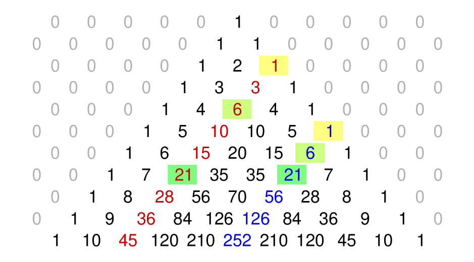
Figure 1. Pascal’s Triangle

In other words, what are the integral solutions to the equation

(2.1) $$\binom{y}{k}=\binom{x}{l}\,,$$

subject to the conditions $1<k\leq y/2$, $1<l\leq x/2$ and $k<l$? The following solutions are known.

$$\binom{16}{2}=\binom{10}{3},\quad\binom{56}{2}=\binom{22}{3},\quad\binom{120}{2}=\binom{36}{3},$$

$$\binom{21}{2}=\binom{10}{4},\quad\binom{153}{2}=\binom{19}{5},\quad\binom{78}{2}=\binom{15}{5}=\binom{14}{6},$$

$$\binom{221}{2}=\binom{17}{8},\quad\binom{F_{2i+2}F_{2i+3}}{F_{2i}F_{2i+3}}=\binom{F_{2i+2}F_{2i+3}-1}{F_{2i}F_{2i+3}+1}\mbox{ for }i=1,2,\ldots,$$

where $F_{n}$ is the $n$-th Fibonacci number.

Equation (2.1) is not a diophantine equation according to our definition, since it depends on $k$ and $m$ in a non-polynomial way. Also, it is way too hard to solve. So we specialize by fixing $k$ and $l$. The cases

$$(k,l)\in\{(2,3),(2,4),(2,6),(2,8),(3,4),(3,6),(4,6),(4,8)\}$$

have already been solved completely, see [7]. Each of these cases requires some deep mathematics of a flavor similar to what is described below. The next interesting case is obviously $(k,l)=(2,5)$, leading to the equation

(2.2) $$\binom{y}{2}=\binom{x}{5}\,,\quad\mbox{or}\quad 60y(y-1)=x(x-1)(x-2)(x-3)(x-4)\,.$$

So we are asking for numbers that occur both in the red and the blue diagonal in Figure 1.

The first step in solving an equation like (2.2) is to go and look for its solutions. We easily find solutions with

$$x=0,1,2,3,4,5,6,7,15\quad\mbox{and}\quad 19\,,$$

and then no further ones. (Only the last two are ‘nontrivial’ in the sense that they satisfy the constraints given above. Also, there are no solutions with $x<0$, since then the right hand side is negative, but the left hand side can never be negative for $y\in{\mathbb{Z}}$.) This now raises the question if we have already found them all, and if so, how to prove it.

This is a good point to look at what is known about the solution set of equations like (2.2) in general. The first important result was proved by Carl Ludwig Siegel in 1929. (See [5, Section D.9] for a proof.)

Theorem 2 (Siegel).

Let $F\in{\mathbb{Z}}[x,y]$. If the solutions to $F(x,y)=0$ cannot be rationally parameterized, then $F(x,y)=0$ has only finitely many solutions in integers.

A rational parameterization of $F(x,y)=0$ is a pair of rational functions $f(t)$, $g(t)$ (quotients of polynomials), not both constant, such that $F(f(t),g(t))=0$ (as a function of $t$). The existence of such a rational parameterization can be algorithmically checked; for our equation it turns out that it is not rationally parameterizable. So we already know that there are only finitely many solutions. In particular, we have a chance that our list is complete. On the other hand, Theorem 2 and its proof are inherently ineffective: we do not get a bound on the size of the solutions, so this result gives us no way of checking that our list is complete. This somewhat unsatisfactory state of affairs did not change until the 1960s, when Alan Baker developed his theory of ‘linear forms in logarithms’ that for the first time provided explicit bounds for solutions of many types of equations. For this breakthrough, he received the Fields Medal. Baker’s results cover a class of equations that contains our equation (2.2). For our case, what he proved comes down to roughly the following.

(2.3) $$|x|<10^{10^{10^{10^{600}}}}\,.$$

This reduces the solution of our equation (2.2) to a finite problem. The inequality in (2.3) gives us an explicit upper bound for $x$. So we only have to check the finitely many possibilities that remain, and we will obtain the complete set of solutions to (2.2). From a very pure mathematics viewpoint, we may therefore consider our problem as solved. On the other hand, from a more practical point of view, we would like to actually obtain the complete list of solutions, and the assertion that it is possible in principle to get it does not satisfy us. To say that the number showing up in (2.3) defies all imagination is a horrible understatement, and one cannot even begin to figure out how long it would take to actually perform all the necessary computations.

However, time did not stop in the 1960s, and with basically still the same method, but with a lot of refinements and improvements thrown in, we are now able to prove the following estimate.

(2.4) $$|x|<10^{10^{600}}\,.$$

You may rightly ask whether something has really been gained, in practical terms. The number of electrons in the universe is estimated to be about $10^{80}$, so we cannot even write down a number with something like $10^{600}$ digits! However, it will turn out that the improvement represented by (2.4) is crucial. But before we can see this, we need to look at our problem from a different angle.

3. A Geometric Interpretation

The idea is to translate our at first sight algebraic problem ((2.2) is an algebraic equation) into a geometric one. An equation $F(x,y)=0$ in two variables defines a subset of the plane, consisting of those points whose coordinates satisfy the equation. If $F$ is a (non-constant) polynomial, this solution set is called a plane algebraic curve. We can draw the curve $C$ corresponding to our equation (2.2) in the real plane ${\mathbb{R}}^{2}$, see Fig. 2. We are now interested in the integral points on $C$, since they correspond to integral solutions to (2.2). The set of integral points on $C$ is denoted $C({\mathbb{Z}})$.

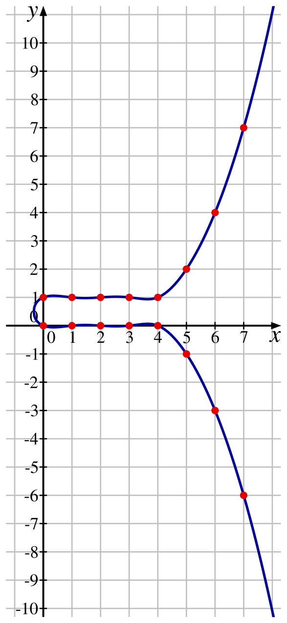
Figure 2. The curve given by (2.2), with some integral points.

This set $C({\mathbb{Z}})$ of integral points on the curve $C$ by itself does not have any useful additional structure. But we can make use of a well-developed theory, called Algebraic Geometry, that studies sets defined by a collection of polynomial equations, and in particular algebraic curves like $C$. This theory tells us that we can embed the curve $C$ into another object $J$, which is not a curve, but a surface. This can be constructed for any curve and is called the Jacobian variety of the curve. The interesting fact about $J$ (and Jacobian varieties in general) is that $J$ is a group. More precisely, there is a composition law on $J$ that is defined in a geometric way and that turns (for example) the set $J({\mathbb{Z}})$ of integral points on $J$ into an abelian group. In a similar spirit as Siegel’s Theorem 2 (and actually preceding it), we have the following important result, valid for Jacobian varieties in general. (See [5, Part C].)

Theorem 3 (Weil 1928).

If $J$ is the Jacobian variety of a curve, then the abelian group $J({\mathbb{Z}})$ is finitely generated.

This means that we can (in principle) get an explicit description of the group $J({\mathbb{Z}})$ in terms of generators and relations. If we have that, we may be able to use the group structure and the geometry in some way to get a handle on the elements of $J({\mathbb{Z}})$ that are in the image of $C$; these correspond exactly to the integral points on $C$.

In general, it is not known whether it is always possible to actually determine explicit generators of a group like $J({\mathbb{Z}})$ in an algorithmic way, although there are some ‘standard conjectures’ whose truth would imply a positive answer. There are methods available that, with some luck, can find a set of generators, but they are not guaranteed to work in all cases. This is the point where the method we are describing may fail in practice. In our specific example, we are lucky, and we can show that $J({\mathbb{Z}})$ is a free abelian group of rank 6:

(3.1) $$J({\mathbb{Z}})={\mathbb{Z}}\,P_{1}+{\mathbb{Z}}\,P_{2}+{\mathbb{Z}}\,P_{3}+{\mathbb{Z}}\,P_{4}+{\mathbb{Z}}\,P_{5}+{\mathbb{Z}}\,P_{6}$$

with explicitly known points $P_{1},\dots,P_{6}\in J({\mathbb{Z}})$.

Let $\iota:C\to J$ denote the embedding of $C$ into $J$. The surface $J$ lives in some high-dimensional space, and we can specify integral points on it by a bunch of coordinates. We can measure the size of such a point by taking the logarithm of the largest absolute value of the coordinates (this tells us roughly how much space we need to write the point down). This gives us a function

$$h:J({\mathbb{Z}})\to{\mathbb{R}}_{\geq 0}$$

called the height. One can show that this height function has the following properties. The first one tells us how the height relates to the size of integral points on our curve.

(3.2) $$h\bigl{(}\iota(x,y)\bigr{)}\approx\log|x|$$

for points $(x,y)\in C({\mathbb{Z}})$ such that $x$ is not very small.

The second property says that the height function behaves well with respect to the group structure on $J$.

(3.3) $$h(n_{1}P_{1}+n_{2}P_{2}+n_{3}P_{3}+n_{4}P_{4}+n_{5}P_{5}+n_{6}P_{6})\approx n_{1}^{2}+n_{2}^{2}+n_{3}^{2}+n_{4}^{2}+n_{5}^{2}+n_{6}^{2}\,.$$

(To be precise, each side can be bounded by an explicit constant multiple of the other one. To be more precise, $h$ is, up to a bounded error, a positive definite quadratic form on $J({\mathbb{Z}})$.)

If we now combine the estimate (2.4) with the properties (3.2) and (3.3) of the height $h$, then we obtain the following statement.

Lemma 4.

If $(x,y)\in C({\mathbb{Z}})$, then we have

$$\iota(x,y)=n_{1}P_{1}+n_{2}P_{2}+n_{3}P_{3}+n_{4}P_{4}+n_{5}P_{5}+n_{6}P_{6}$$

with coefficients $n_{j}\in{\mathbb{Z}}$ satisfying $|n_{j}|<10^{300}$.

Of course, the bound $10^{300}$ given here is not precise; a precise bound can be given and is of the same order of magnitude.

The conclusion is that using the additional structure we have on $J$ enables us to reduce the size of the search space from about $10^{10^{600}}$ to ‘only’ $10^{1800}$ (there are six coefficients $n_{j}$ with about $10^{300}$ possible values each). This is, of course, still much too large to check each possibility (think of the electrons in the universe), but, and this is the decisive point, the numbers $n_{j}$ we have to deal with can be represented easily on a computer, and we can compute with them!

4. Needles in a Haystack

We now have an enormous haystack

$$H=\left\{(n_{1},n_{2},n_{3},n_{4},n_{5},n_{6})\in{\mathbb{Z}}^{6}:|n_{j}|<10^{300}\right\}$$

of about $10^{1800}$ pieces of grass that contains a small number of needles. We want to find the needles. Instead of looking at each blade of grass in the haystack, we can try to solve this problem faster by finding conditions on the possible positions of the needles that rule out large parts of the haystack. This is the point where we make use of the fact that the group law on $J$ is defined via geometry. Our objects $C$, $J$ and $\iota$ are defined over ${\mathbb{Z}}$, therefore it makes sense to consider their defining equations modulo $p$ for prime numbers $p$. We denote the field ${\mathbb{Z}}/p{\mathbb{Z}}$ of $p$ elements by ${\mathbb{F}}_{p}$. The sets of points with coordinates in ${\mathbb{F}}_{p}$ that satisfy these defining equations mod $p$ are denoted by $C({\mathbb{F}}_{p})$ and $J({\mathbb{F}}_{p})$. Then for all but finitely many $p$ (and the exceptions can be found explicitly), $J({\mathbb{F}}_{p})$ is again an abelian group, and it contains the image $\iota(C({\mathbb{F}}_{p}))$ of $C({\mathbb{F}}_{p})$. The group $J({\mathbb{F}}_{p})$ is finite, and so is the set $C({\mathbb{F}}_{p})$; both can be computed. Furthermore, the following diagram commutes, and the geometric nature of the group structure implies that the right hand vertical map is a group homomorphism.

The vertical maps are obtained by reducing the coordinates of the points mod $p$. The diagonal map $\alpha_{p}$ is again a group homomorphism, determined by the image of the generators $P_{1},\dots,P_{6}$ of $J({\mathbb{Z}})$. The following is now clear.

Lemma 5.

Let $(x,y)\in C({\mathbb{Z}})$ and $\iota(x,y)=n_{1}P_{1}+\cdots+n_{6}P_{6}$. Then

$$\alpha_{p}(n_{1},n_{2},n_{3},n_{4},n_{5},n_{6})\in\iota_{p}\bigl{(}C({\mathbb{F}}_{p})\bigr{)}\,.$$

The subset $\Lambda_{p}=\alpha_{p}^{-1}\bigl{(}\iota_{p}(C({\mathbb{F}}_{p}))\bigr{)}\subset{\mathbb{Z}}^{6}$ is (usually, when $\alpha_{p}$ is surjective) a union of $\#C({\mathbb{F}}_{p})$ cosets of a subgroup of index $\#J({\mathbb{F}}_{p})$ in ${\mathbb{Z}}^{6}$. Since one can show that $\#C({\mathbb{F}}_{p})\approx p$ and $\#J({\mathbb{F}}_{p})\approx p^{2}$ (reflecting dimensions $1$ and $2$, respectively), we see that the intersection of our haystack $H$ with $\Lambda_{p}$ has only about $1/p$ times as many elements as the original haystack. This does not yet help very much, but we can try to combine information coming from many primes. If $S$ is a (finite, but large) set of prime numbers, then we set

$$\Lambda_{S}=\bigcap_{p\in S}\Lambda_{p}\quad\mbox{and obtain}\quad\iota\bigl{(}C({\mathbb{Z}})\bigr{)}\subset\Lambda_{S}\cap H\,.$$

If we make $S$ sufficiently large (about a thousand primes, say), then it is likely that the set on the right hand side is quite small, so that we can easily check the remaining possibilities. The idea is that the reductions of the haystack size we obtain from several distinct primes should accumulate, so that we can expect a reduction by a factor which is roughly the product of all the primes in $S$.

We have to be careful to select the primes in a good way so that the description of the sets $\Lambda_{S}$ we encounter on the way stays within a reasonable complexity. It is, however, indeed possible to make a good selection of primes and to implement the actual computation of $\Lambda_{S}$ in a reasonably efficient manner, so that a standard PC (standard as of 2008) can perform the calculations in less than a day. We finally obtain the result we were suspecting from the beginning.

Theorem 6 (Bugeaud, Mignotte, Siksek, Stoll, Tengely).

Let $x,y$ be integers satisfying

$$\binom{y}{2}=\binom{x}{5}\,.$$

Then  $x\in\{0,1,2,3,4,5,6,7,15,19\}\,.$

A detailed description of the method (explained using the different example equation $y^{2}-y=x^{5}-x$) can be found in [2].

References

- [1] Beck, M.; Pine, E.; Tarrant, W.; Yarbrough Jensen, K.: New integer representations as the sum of three cubes, Math. Comp. 76, no. 259, 1683–1690 (2007)
- [2] Bugeaud, Y.; Mignotte, M.; Siksek, S.; Stoll, M.; Tengely, Sz.: Integral points on hyperelliptic curves, Algebra Number Theory 2, No. 8, 859–885 (2008)
- [3] Hilbert, D.: Mathematische Probleme. Vortrag, gehalten auf dem internationalen Mathematiker-Congress zu Paris 1900. (German) Gött. Nachr. 1900, 253–297 (1900).
- [4] Hilbert, D.: Mathematical problems. Reprinted from Bull. Amer. Math. Soc. 8 (1902), 437–479. Bull. Amer. Math. Soc. (N.S.) 37 (2000), no. 4, 407–436 (electronic)
- [5] Hindry, M.; Silverman, J.H.: Diphantine Geometry. An Introduction, Springer GTM 201, New York etc., 2000.
- [6] Matiyasevich, Y.: Hilbert’s Tenth Problem, MIT Press, Cambridge, Massachusetts, 1993.
- [7] Stroeker, R.J.; de Weger, B.M.M.: Elliptic binomial Diophantine equations, Math. Comp. 68, 1257–1281 (1999).