Statistics for surface modes of nanoparticles with shape fluctuations

Abstract

We develop a numerical method for approximating the surface modes of sphere-like nanoparticles in the quasi-static limit, based on an expansion of (the angular part of) the potentials into spherical harmonics. Comparisons of the results obtained in this manner with exact solutions and with a perturbation ansatz prove that the scheme is accurate if the shape deviations from a sphere are not too large. The method allows fast calculations for large numbers of particles, and thus to obtain statistics for nanoparticles with random shape fluctuations. As an application we present some statistics for the distribution of resonances, polariziabilities, and dipole axes for particles with random perturbations.

I Introduction

The excitation of surface plasmons can cause strong interaction between light and metallic nanoparticles. These plasmons are hybrid modes of the electromagnetic field and the electron gas and are confined to the surface of the particle. They give rise to an enhancement of the incident field by several orders of magnitude Kreibig_Vollmer ; Bohren_Huffmann ; Hao_Schatz . This enhancement enables a variety of applications ranging from the well-established surface-enhanced Raman spectroscopy (SERS), which allows the detection of even a single molecule Nie_Emory ; Kneipp , to the emerging field of plasmonics Maier_Atwater ; Ozbay , which has led to prototypes of plasmonic waveguides which effectuate optical energy transfer below the diffraction limit Maier_Atwater ; Brongersma ; Maier ,

A simple realization of a plasmonic waveguide is a chain of metallic spheres. A surface plasmon mode, typically a dipole mode, of the first sphere of the chain is excited and the scattered field of this first particle excites a surface mode in a sphere nearby and so the excitation can travel through the chain. There are two crucial points for an efficient transport: The spatial structure of the scattered field in the region of the neighboring sphere must allow for an efficient excitation of the favored mode, and the overlap of the resonances of the bordering spheres has to be big enough. Since any realization of a sphere will deviate from an ideal one, thus introducing random fluctuations, it is important to estimate the typical magnitude of such deviations which still allow for an efficient transport. Therefore a simple and efficient numerical method for approximating the surface modes of the sphere-likes particles is needed.

There are many numerical methods for the determination of the electromagnetic field in the present of nanosized scatterers, like the finite difference time domain approach (FDTD), or so called semi–analytical methods based on expansions into special function systems like the multiple multipole method (MMP), or the discrete dipole approximation (DDA), see, e.g., Wriedt ; Kahnert for reviews. Essentially, all methods able to calculate the fields also allow to determine the surface modes. For example, in Noguez the DDA is used for the determination of the surface modes of nanoparticles, and in Abajo_Aizpurua ; Abajo_Aizpurua2 a boundary integral approach is proposed, which focuses on the surface modes, and has been used in Hohenester_Krenn to determine the surface modes of single and coupled spheres, cylinders and cube–like nanoparticles.

Here we use a semi-analytical approach based on an expansion of the potentials into spherical harmonics, i.e., into modes $r^{l}Y^{m}_{l}(\theta,\phi)$ and $r^{-(l+1)}Y^{m}_{l}(\theta,\phi)$, and on the determination of the expansion coefficients by the physically motivated projection of the boundary conditions onto the modes $r^{l}Y^{m}_{l}(\theta,\phi)$. See also (mish02, , Sec. 6) for a review of various ways to determine expansions from the boundary conditions in a variety of related problems. For nonspherical particles, our approach corresponds to an expansion into non–orthogonal modes and therefore is similar to the usage of the Rayleigh hypothesis in the theory of scattering in optics, where the scattered field at a perturbed interface is likewise expanded in the solutions of the scattered field of the unperturbed one Nieto . It is known that such expansion methods may fail if the deviations from the ideal geometry become too large, see, e.g., Ramm and the references therein. Nonetheless, additional to its simplicity and easy implementation the distinct advantage of our approach is its computational efficiency for nearly spherical particles. Thus it allows to calculate the surface modes for many realizations of randomly distorted nanospheres and so to statistically characterize their optical responses.

The paper is organized as follows: The numerical method is explained in Sec. II, and validated in Sec. III, using the cases of an ellipsoid and of a sphere with certain shape distortions as benchmarks. In Sec. IV we give a statistical study of the optical response of spheres and spheroids with random perturbations.

II The scheme

We are interested in the surface modes of sphere-like nanoparticles, described as some bounded domain $\Omega\subset{\mathbb{R}}^{3}$, with boundary ${\partial}\Omega$. We restrict ourselves to particles that are small compared to the relevant wavelengths and therefore employ the quasi-static approximation. In order to determine their surface modes we consider an excitation from infinity (described by the potential $\Phi_{ext}$), and calculate the potential inside ($\Phi_{-}$) and outside ($\Phi_{+}$) the particle. These potentials fulfill the Laplace equation

$$\Delta\Phi_{\pm}(\bm{x})=0\quad\text{for }\bm{x}\not\in{\partial}\Omega.$$ (1)

In addition, the boundary conditions on the surface ${\partial}\Omega$ of the particle are

$$\Phi_{+}(\bm{x})=\Phi_{-}(\bm{x})\quad\text{for }\bm{x}\in{\partial}\Omega,$$ (2)

$$\partial_{n}\Phi_{+}(\bm{x})=\epsilon\partial_{n}\Phi_{-}(\bm{x})\quad\text{for }\bm{x}\in{\partial}\Omega,$$ (3)

with the outward normal derivative $\partial_{n}$ and the permittivity $\epsilon$ of the particle. The boundary condition (3) implies that the particle is surrounded by vacuum, and is homogeneous, isotropic, and non-magnetic; the dielectric properties are assumed to be local.

There are two different methods to determine the surface modes of a nanoparticle from (1)-(3). The first is to assume that the potential vanishes at infinity, i.e. to calculate the modes of the particle that can be present without an external excitation. In this case the problem can be reformulated as an eigenvalue problem with a real plasmonic eigenvalue $\epsilon$ for which a nontrivial solution of Eqs. (1)-(3) with $\lim\limits_{\|\bm{x}\|\rightarrow\infty}|\Phi_{+}(\bm{x})|=0$ exists Grieser . In this interpretation the variable $\epsilon$ in (3) is not regarded as the generally complex permittivity of the particle, but rather as a real eigenvalue. The second method is to study the system (1)-(3) with an external excitation and thus to regard the $\epsilon$ in (3) as the complex permittivity $\epsilon(\omega)$ of the particle. The system is then solved for different values of the permittivity and a solution is called a surface mode if the field inside and around the particle is enhanced. If the imaginary part of the permittivity does not vary too much, then the enhanced fields occur when the real part of $\epsilon$ is equal to a plasmonic eigenvalue. Thus the terms plasmonic eigenvalue and resonant value are closely related and will be used interchangeably. In general there will be a difference in the number of eigenvalues and resonant values. While there is a infinite number of eigenvalues, the used excitation will choose some of these eigenvalues and only for these an enhanced field will appear.

We study the response of a particle to an external field and assume that the potential at infinity equals the potential of the excitation;

$$\lim_{\|\bm{x}\|\rightarrow\infty}|\Phi_{+}(\bm{x})-\Phi_{ext}(\bm{x})|=0.$$ (4)

The basic idea is to expand the potential inside and outside the particle into spherical modes which automatically fulfill the Laplace equation (1),

$$\Phi_{-}(\bm{x})=\sum\limits_{l=0}^{\infty}\sum_{m=-l}^{l}\alpha_{l,m}r^{l}Y^{m}_{l}(\theta,\phi),$$ (5)

and $\Phi_{+}=\psi_{+}+\Phi_{ext}$ with

$$\psi_{+}(\bm{x})=\sum\limits_{l=0}^{\infty}\sum_{m=-l}^{l}\beta_{l,m}r^{-(l+1)}Y^{m}_{l}(\theta,\phi)$$ (6)

and $\Phi_{ext}(\bm{x})=\sum\limits_{l=0}^{\infty}\sum\limits_{m=-l}^{l}\gamma_{l,m}r^{l}Y^{m}_{l}(\theta,\phi)$. Here $\bm{x}=r\big{(}\cos(\phi)\sin(\theta),\sin(\phi)\sin(\theta),\cos(\theta)\big{)}^{t}$ and the familiar spherical harmonics are denoted by $Y^{m}_{l}(\theta,\phi)=P^{m}_{l}(\cos\theta)\text{e}^{{\rm i}m\phi}$: For $m{\geq}0$, the associated Legendre polynomials are $\displaystyle P_{l}^{m}(s)=c_{l}^{m}\frac{1}{2^{l}l!}(1{-}s^{2})^{m/2}\left(\frac{{\rm d}}{{\rm ds}}\right)^{l+m}(s^{2}{-}1)^{l}$ with the scale factors $c^{m}_{l}=(-1)^{m}\sqrt{\frac{2l+1}{4\pi}}\sqrt{\frac{(l-m)!}{(l+m)!}}$, and $P^{m}_{l}:=(-1)^{m}P^{-m}_{l}$ for $m<0$.

From (4) the coefficients $\gamma_{l,m}$ are defined by the excitation potential. Thus it remains to calculate the coefficients $\alpha_{l,m}$ and $\beta_{l,m}$ from (2) and (3). In order to do this we use the following numerical scheme. First we truncate to $|l|\leq N$ such that $(N+1)^{2}$ coefficients $\alpha_{l,m}$ and $\beta_{l,m}$ have to be calculated. To get the required $2(N+1)^{2}$ equations we project the boundary conditions (2) and (3) onto the modes $r^{l}Y^{m}_{l}(\theta,\phi)$ with degree equal to or less than $N$. In detail, we require

$$\int_{{\partial}\Omega}(\Phi_{-}-\psi_{+})\,r^{l}Y^{m}_{l}(\theta,\phi)\,{\rm d}S$$ (7)

$$=\int_{{\partial}\Omega}\Phi_{Ext}\,r^{l}Y^{m}_{l}(\theta,\phi)\,{\rm d}S,$$

$$\int_{{\partial}\Omega}(\epsilon{\partial}_{n}\Phi_{-}-{\partial}_{n}\psi_{+})\,r^{l}Y^{m}_{l}(\theta,\phi)\,{\rm d}S$$ (8)

$$=\int_{{\partial}\Omega}({\partial}_{n}\Phi_{Ext})\,r^{l}Y^{m}_{l}(\theta,\phi)\,{\rm d}S.$$

This yields a system of the form

$$(M_{1}+\epsilon M_{2})U=M_{3}G$$ (9)

where $M_{1},M_{2},M_{3}\in{\mathbb{C}}^{2(N+1)^{2}\times 2(N+1)^{2}}$ are matrices which depend only on the geometry of the particle, $G\in{\mathbb{C}}^{2(N+1)^{2}}$ depends only on the $\gamma_{lm}$, and $U\in{\mathbb{C}}^{2(N+1)^{2}}$ contains the unknown coefficients $\alpha_{lm}$ and $\beta_{lm}$.

For a sphere $S_{r_{0}}$ of radius $r_{0}$ the spherical harmonics $Y^{m}_{l}$ are an orthogonal (orthonormal if $r_{0}=1$) basis of $L^{2}({\partial}S_{r_{0}})$. Thus, (9) decouples in the case of a sphere (becomes block diagonal, see A for the precise structure) and yields $(N+1)^{2}$ exact solutions of (1)–(3). For a perturbed sphere the $Y^{m}_{l}$ are no longer orthogonal, and the physically motivated idea of projecting onto the modes $r^{l}Y^{m}_{l}$ (instead of, e.g., projecting onto the spherical harmonics $Y^{m}_{l}$, which at first might appear more natural) is as follows: we may expect the fields to be localized near parts of ${\partial}\Omega$ with high curvature, and for perturbations of spheres (of radius $r_{0}$) these occur most naturally for parts bulging out, i.e., for $r>r_{0}$. Thus, to minimize the error, it appears reasonable to weight the spherical harmonics as test functions in (7),(8) with $r^{l}$. This also complies with the folklore rule to use the same functions as test functions and as ansatz function. On the other hand, this rule is rather ambiguous here since we have $(N+1)^{2}$ more ansatz functions, namely $r^{-(l+1)}Y^{m}_{l}$. However, these tend to localize near “flat” parts of the perturbed sphere and are therefore less useful as test functions. We evaluated all three sets of test functions $(r^{l}Y^{m}_{l})_{l,m}$, $(Y^{m}_{l})_{l,m}$, and $(r^{-(l+1)}Y^{m}_{l})_{l,m}$, against available exact solutions for spheroids (see Sec. III) and found that $(r^{l}Y^{m}_{l})$ works best while $(Y^{m}_{l})$ and even more so $(r^{-(l+1)}Y^{m}_{l})$ yield slower convergence.

As already pointed out in the Introduction, expansions like those given by Eqs. (5) and (6) are conceptually related to the Rayleigh hypothesis, and may fail to converge if the deviation of the geometry considered from the ideal geometry is too large. Therefore it is of great importance to test the method against known exact solutions, and to control the error. As shown below, for the present problem it turns out that already moderate $N$ yield quite accurate results if the deviations from a sphere are not too large. The achievable accuracy, however, also depends on the quantities one wants to compute. We find that typically $N=7$, which yields $M_{j}\in{\mathbb{C}}^{128\times 128}$, is sufficient to calculate the resonant value of $\epsilon$ with high accuracy.

The generation of the matrices $M_{j}$ is the most expensive part of the scheme since each entry requires the evaluation of surface integrals similar to the ones in Eqs. (7) and (8). However, once the matrices $M_{j}$ are generated, for any given $\Phi_{ext}$ we only need to first calculate the coefficients $\gamma_{lm}$ and then solve some rather small linear system with given $\epsilon$. In particular, the scheme allows for a fast parameter scan when solving the system (9) for different $G$, i.e., when rotating the incident field. For fixed $\epsilon$ we may also define a T–matrix $T=(M_{1}+\epsilon M_{2})^{-1}M_{3}$ to obtain $U=TG$. The calculation of the $\gamma_{lm}$ is quite simple; for instance, for a constant field in $(x,y,z)^{t}$-direction the coefficients are $\gamma_{lm}=0$ for $l\neq 1$ and $\gamma_{1,-1}=-x-{\rm i}y$, $\gamma_{1,0}=z$ and $\gamma_{1,1}=x-{\rm i}y$.

We use the GNU Scientific Library GSL for the spherical harmonics and the Cuba library CUBA for calculating the projection integrals (7),(8). The linear system (9) is then solved with a standard method from LAPack LAPack .

III Comparison with exact solutions and a perturbation ansatz

As test cases for our scheme we consider the surface modes of an ellipsoidal particle, for which an exact solution exists Bohren_Huffmann , and the case of a sphere with certain Gaussian perturbations. For the latter we compare our results with the results of a recently developed perturbation-theoretical ansatz Perturbation .

III.1 Surface modes of an ellipsoid

We start with a spheroid, i.e. an ellipsoid with two identical semi–axes. The spheroid is oriented such that the two identical axes are along the $x$- and $y$- axis of the coordinate system. Furthermore, we choose the semi-diameter in $x$- and $y$- direction as $1$. Thus the geometry of the test case is described by one parameter $R$, the semi–axis in $z$-direction. As the dipole modes of a sphere are excitable by a constant field, and we are interested primarily in dipole-like modes, we use a constant incident field in the test cases.

Considering a constant incident field in $z$-direction, the exact solution for the resonant value of the permittivity $\epsilon$ is Bohren_Huffmann

$$\epsilon(R)=1-\frac{1}{L(R)}$$ (10)

with the depolarization coefficient $L(R)$ given by

$$L(R)=\frac{R}{2}\int\limits_{0}^{\infty}\,\text{d}s\frac{1}{(s+R)^{2}\sqrt{2(s+1)(s+R^{2})}}.$$ (11)

Numerically we determine the resonances as follows: After calculating the matrices $M_{j}$ we solve Eq. (9) for different values of $\epsilon$, and define the resonant value as that value of $\epsilon$ which produces the biggest dipole-like near field, i.e., we search the value of $\epsilon$ which maximizes $\sqrt{|\beta_{1,-1}|^{2}+|\beta_{1,0}|^{2}+|\beta_{1,1}|^{2}}$.

Figure 1: Comparison of the exact resonant values for a spheroid with the ones calculated within our approach for different $N$, and an incident field oriented along the $x$-axis (a), and the $z$-axis (b). In the later Fig. 4, where we show the polarizability of a spheroids, the dependence of the resonant values on $N$ can be seen in more detail.

In Fig. 1 we compare the resonances thus obtained numerically with the exact ones, for different $N$ and for two different incident fields. The results are remarkably good, even for small $N$. Indeed, for an incident field in $z$-direction and $R=1.5$, for example, the exact result figures as $\epsilon\approx-3.29$, while the numerical procedure with $N=1$ gives $\epsilon=-3.18$, and differs from the exact result by less than $10^{-2}$ with $N=7$. Thus, for the calculation of the resonant values our method gives accurate results even with only few spherical harmonics, and even when the shape deviates significantly from that of a sphere.

On the other hand, the method is in general not well suited for the calculation of the fields with high accuracy if the deviations from the sphere become large. For illustration, we first show in Fig. 2 (a) the potentials inside and outside a spheroid with $R=1.4$, for an incident field in $z$-direction. The linescan in (b) shows that along the particular line indicated in (a) the boundary conditions (2), (3) are reasonably well fulfilled for $N=7$, while the jumps for $N=1$ indicate that in this case $N=1$ is not sufficient, as expected.

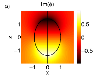
Figure 2: (Color online) (a) Calculated potentials inside and around a spheroid for $R=1.4$ and $N=7$. The imaginary part of the potential is plotted for the resonant value of the permittivity and the potential is normalized such that the maximum of the imaginary part is $1$. The shape of the spheroid is indicated by the black ellipse. The linescans in (b) are taken for $x=0$; the one with $N=1$ is shifted downwards by $1$ for clarity.

From a systematic viewpoint, a more relevant basic check of the accuracy of the potentials is the total relative error in Eqs. (2), (3). In Fig. 3 we plot the $L^{2}$–norms of these errors, again as functions of $R$ and $N$, henceforth denoted by

$$e_{1}:=\frac{2\|\Phi_{+}-\Phi_{-}\|}{\|\Phi_{+}\|+\|\Phi_{-}\|},\quad e_{2}:=\frac{2\|{\partial}_{n}\Phi_{+}-\epsilon{\partial}_{n}\Phi_{-}\|}{\|{\partial}_{n}\Phi_{+}\|+\|{\partial}_{n}\Phi_{-}\|},$$

where $\|f\|=(\int_{{\partial}\Omega}|f|^{2}\,{\rm d}S)^{1/2}$. For $R$ close to $1$, say $0.8\leq R\leq 1.3$, we find that $e_{1}$ and $e_{2}$ are small and decrease monotonously in $N$. However, $e_{1,2}$ become large rather quickly when $R$ falls outside this range. Moreover, they then no longer decay in $N$, which we attribute to a failure analogous to that of the Rayleigh hypothesis for such strongly deformed spheres.

Figure 3: (a) $L_{2}$-norm of the boundary condition (2), and (b) of the condition (3), for the indicated $N$.

Similar effects can be observed for various other test particles: The approximation of resonant values of $\epsilon$ is typically much better than $e_{1,2}$. Thus the performance of the method strongly depends on what one wants to compute. As a rule of thumb we find that for $e_{1,2}\leq 0.2$ we obtain very good approximations of the resonant values, and also of the polarizabilities and of the dipole axes, as shown below; these three observables are the quantities we are mainly interested in. Therefore we have made sure that in all calculations presented below we have $e_{1,2}<0.1$. For the solution shown in Fig. 2 with $N=7$ we have $e_{2}$ slightly larger than $0.1$, so that this solution would be discarded.

Another quantity of immediate physical interest is the polarizability $\alpha$ which relates the incident field ($\bm{E}_{ext}$) to the excited dipole moment ($\bm{p}_{ex}$). In general this quantity is a tensor, but for the case of a spheroid with an incident field oriented along one of the principal axes the polarizability is a scalar , i.e., $\bm{p}_{ex}=\epsilon_{0}\alpha\bm{E}_{ext}$.

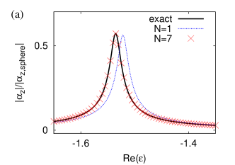
Figure 4: (Color online) Comparison of the exact and numerically calculated polarizability of a spheroid with $R=0.8$ (a). The polarizability is normalized to the one of a sphere with radius $1$ and a dielectric function of $-2+0.01\text{i}$. In the right panel (b) the coefficients of the spherical harmonics are presented for $N=7$ and a value of $\epsilon$ close to the resonant value.

In Fig. 4(a) the exact and the numerically calculated polarizability of a spheroid with $R=0.8$ is depicted, more precisely its absolute value for an incident field in $z$-direction, i.e. $|\alpha_{z}|\propto\sqrt{|\beta_{1,-1}|^{2}+|\beta_{1,0}|^{2}+|\beta_{1,1}|^{2}}$. The width and the magnitude of the polarizability are excellently reproduced by our scheme and the agreement between the exact solution and the numerical one is very good already for $N\geq 3$, and even for $N=1$ the approximation already reproduces the shape of the resonance quite well. Fig. 4(b), which depicts the coefficients $\beta_{l,m}$ for the expansion (6), shows that the dominant part of the field stems from $l=1$, but higher spherical harmonics also give non-negligible contributions.

We have also checked our scheme against the exact solution for an ellipsoid with three different semi-diameters, and an incident field that is not oriented along one of the principal axes. Again the agreement between the exact solution Bohren_Huffmann and our results is very good as long as the semi-diameters are not too different.

III.2 Surface modes of a sphere with a perturbation

In Sec. IV we perform a statistical analysis for the surface modes of nanoparticles with a random shape, described by

$$r(\theta,\phi)=1+s\sum\limits_{i=1}^{n}h_{i}\exp\left(-0.5\left(\frac{{\rm dist}(\theta_{i},\phi_{i};\theta,\phi)}{w_{i}}\right)^{2}\right)$$ (12)

where $s$ is a scaling factor, dist$(\theta_{i},\phi_{i};\theta,\phi)$ is the Euclidean distance between two points on the unit sphere, one specified by $\theta_{i}$ and $\phi_{i}$ and the other by $\theta$ and $\phi$. In these later studies, $\theta_{i}$, $\phi_{i}$, $h_{i}$ and $w_{i}$ will be randomly distributed. Thus, the nanoparticles then are spheres with $n$ Gaussian perturbations with height $h_{i}$ and width $w_{i}$. In order to assess our method for such cases, we first consider a particle with three perturbations, study how the resonance is shifted by varying the scaling parameter $s$, and compare the results with those of a perturbation ansatz for the surface modes of a nanoparticle Perturbation .

For the perturbation ansatz a geometry close to the given one is needed, for which an exact solution for the surface modes exists. In the following that geometry is called the ideal geometry, and the geometry for which the surface modes are to be calculated is called the perturbed geometry. It is assumed that the perturbation strength is described by a scalar parameter. In our case the ideal geometry is the unit sphere and the parameter that characterizes the deviation from the sphere is the scaling amplitude $s$. When making the perturbation ansatz the resonant values $\epsilon(s)$ are expanded in a series with respect to $s$:

$$\epsilon(s)=\epsilon(0)+s\dot{\epsilon}(0)+\frac{s^{2}}{2}\ddot{\epsilon}(0)+\cdots.$$ (13)

In Ref. Perturbation an explicit formula for $\dot{\epsilon}$ is presented against which we can compare our numerical results. Since the dipole mode of a sphere is threefold degenerate, there are in general three different values of $\dot{\epsilon}$, characterizing the three dipole-like modes.

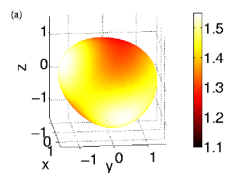
Figure 5: (Color online) Sketch of the used perturbed sphere (a), and the corresponding resonant values of $\epsilon$ (b). The plot (a) refers to a scaling factor of $s=0.5$; the color scale depicts the distance from a point on the surface to the center of the underlying unit sphere. The resonant values in (b) are calculated with $N=7$; the inset shows a blow-up near $s=0$.

The test particle with three Gaussian perturbations is depicted in Fig. 5(a), whereas (b) compares the results provided by (9) with the perturbation method. We only present the results for $N=7$ but remark that the results are stable for $N\geq 5$. There is a very good agreement between the projection and the perturbation method for small $s$. As expected there are deviations for larger scaling factors, because these are beyond the scope of the (first order) perturbation method.

For $s\geq 0.4$ more than three resonances occur, notably one with a real part of the permittivity of about $-1.6$. By plotting the potential (or alternatively inspecting the expansion coefficients $\beta_{l,m}$) we find that these modes are shifted and perturbed quadrupole modes of the unperturbed sphere, which due to the perturbations can be excited by a constant field. For the unperturbed sphere these occur at $\text{Re}(\epsilon)=-1.5$. Of course these modes are in principle present in all cases, but it depends on the respective geometry if these modes could be excited effectively by a constant field.

To conclude the test of our scheme: Already with quite few spherical harmonics (typically $N\leq 7$), and even if the errors $e_{1,2}$ in the boundary conditions are significant, the numerical data for the resonant values and the polariziabilities provided by our method are stable and in remarkable agreement with exact solutions (if available), or with the results of the perturbation ansatz.

IV Particles with randomly distributed Gaussian perturbations

We now assume that we are given a set of nominally identical nanospheres which suffer from uncontrolled shape imperfections induced during the fabrication process. The task then is to characterize the optical properties of this set in a statistical sense. Ideally, one would have at least a good idea how the imperfections are distributed, based on an inspection of a representative number of specimen, then generate a corresponding ensemble, and compute the resonances of each individual member. Since we are not considering any particular case, here we simply assume that the random shape fluctuations correspond to Gaussian distortions as described by Eq. (12). We start with $n=4$, set $s=1$, and choose randomly distributed $\theta_{i}$, $\phi_{i}$, $h_{i}$, and $w_{i}$ with $i=1,\ldots,4$. The positions of the distortions, described by the angles $\theta_{i}$ and $\phi_{i}$, are uniformly distributed on the sphere, $h_{i}$ is normally distributed with a mean of $0.2$ and a standard deviation of $0.1$; the normally distributed widths $w_{i}$ have a mean value of $\mu_{w}=0.7$ and a standard deviation of $\sigma_{w}=0.3$. Clearly, perturbations with a negative width $w_{i}$ are discarded, and we admit only perturbations with $\frac{h_{i}}{w_{i}}\leq 2$ in order to avoid sharp peaks. Therefore each realization is a sphere with four or less perturbations.

In order to get significant results we generate 1000 realizations of the perturbed sphere, calculate for each realization the matrices $M_{i}$, and solve the system of equations (9) for 100 different incident fields, i.e. we consider 100000 cases. We choose $N=7$, and require $e_{1,2}\leq 0.1$ as explained in Sec. III.1, which has resulted in an ensemble with 42829 members.

In Fig. 6(a) we present a histogram of the resonant values of the real part of the permittivity. Here we count a peak in the absolute value $|\alpha_{in}|$ of the polarizability of a particle as a resonance if $|\alpha_{in}|$ is at least $0.1$ times the value $|\alpha_{in,sphere}|$ of a perfect sphere. $H_{\epsilon}$ denotes the number of the resonances in the corresponding interval of $\text{Re}(\epsilon)$ divided by the number of particles. In the following pictures $H_{\alpha}$ and $H_{\theta}$ are defined in an analogous way. As seen in Fig. 6(a) the shape fluctuations result in a relatively broad distribution of the resonant values around the unperturbed value $\text{Re}(\epsilon)=-2$, and the maximum is shifted to a slightly bigger value.

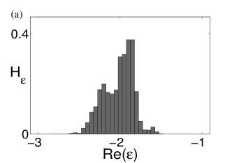
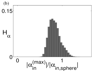
Figure 6: Histogram of the resonant values Re$(\epsilon)$ for the ensemble of perturbed spheres (a), and histogram of the magnitude of the maximum dipole moment $\alpha_{in}^{(max)}$ (b).

Not only the position of the resonance is of interest, but also the magnitude of the induced dipole moment. Therefore we present in Fig. 6(b) a histogram of this magnitude, considering for each ensemble member only the resonance with the largest dipole moment. Due to the fact that the polarizability of a sphere scales with its volume and a typical realization of our perturbed spheres is somewhat bigger than a sphere with radius $1$, we normalize the polarizability to that of a sphere with the same volume as the perturbed one. In the large majority of cases the polarizability of the perturbed sphere is smaller than that of the unperturbed one. This is due to the fact that for the sphere there are no principal axes. Therefore the polarizability is independent of the direction of the incident field, and for any field the induced dipole moment points into the direction of the incident field. But if the symmetry of the sphere is destroyed by the perturbations, there are three distinguished principal axes with different resonant values of the permittivity. So for a fixed permittivity in general only one resonant condition is matched and therefore essentially only the part of the incident field that points into the direction of the corresponding principal axis contributes significantly to the induced dipole moment. This results in an induced dipole moment which typically is smaller than that of a perfect sphere, and is not parallel to the incident field.

In a plasmonic waveguide, consisting of a chain of metallic nanoparticles, a random angle between the induced dipole moment $\bm{p}$ and the incident field $\bm{E}_{ext}$ influences an efficient transport, because the near field of one particle should excite the neighboring particle. Therefore designing a plasmonic waveguide requires the knowledge of the spatial structure of the near field. Because a sphere has no principal axes, any arbitrarily small perturbation will pick three axes and therefore affects the orientation of the induced dipole. Thus, with perturbed spheres we may expect that there are only very few cases in which $\bm{p}$ is nearly parallel to $\bm{E}_{ext}$. To illustrate this quantitatively, we present histograms of the angle between $\bm{p}$ and $\bm{E}_{ext}$ in Fig. 7. In Fig. 7(a) we consider all resonances, whereas in Fig. 7(b) only the biggest resonance for every member is used. The main result is that realizations with $\bm{p}$ nearly parallel to $\bm{E}_{ext}$ are indeed negligible, and the orientation of the dipole relatively to the external field is nearly random. This can be seen from the solid line in Fig. 7(a), proportional to $\sin(\theta)$, which corresponds to a completely random choice of the orientation of the dipoles. This figure also illustrates that the only cases which are suppressed when the spheres are perturbed are those in which $\bm{p}$ and $\bm{E}_{ext}$ are almost perpendicular.

As expected, when only the largest resonances are considered the angle is typically smaller because, as already pointed out, in a resonant situation only that part of the incident field contributes that is parallel to the according dipole axis. Moreover, the distribution of this angle, shown in Fig. 7(b), is quite broad, which demonstrates the substantial variability in the spatial structure of the field around our perturbed spheres.

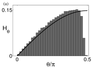
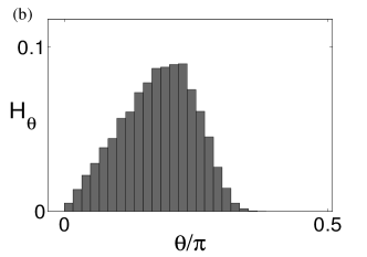
Figure 7: Histogram of the orientation (relative to $\bm{E}_{ext}$) of the induced dipole moment for all resonances (a), and only the biggest ones (b). The solid line in (a) is obtained if the orientation of the dipole axis is entirely random.

Therefore, we now consider the surface modes of perturbed spheroids. As spheroids already have at least one distinguished principal axis, we expect that perturbations of a spheroid do not have such a strong effect on the orientation of the induced dipoles. We employ the same kind of Gaussian perturbations, but now the unperturbed particle is a spheroid with semi-axes $R_{x}=1$, $R_{y}=1$, and $R_{z}=1.2$. Hence, the shape of a particle is described by

$$r(\theta,\phi)= \left[(\sin\theta)^{2}+\left(\frac{\cos\theta}{1.2}\right)^{2}\right]^{-0.5}$$ (14)

$$+\sum\limits_{i=1}^{n}h_{i}\exp\left(-0.5\left(\frac{{\rm dist}(\theta_{i},\phi_{i};\theta,\phi)}{w_{i}}\right)^{2}\right).$$

Again, $\theta_{i}$ and $\phi_{i}$ are uniformly distributed on a sphere, $h_{i}$ are normally distributed with a mean value of $0.2$ and a standard deviation of $0.1$, and the normally distributed $w_{i}$ have a mean value of $0.7$ and a standard deviation of $0.3$. We consider 10000 realizations of the spheroid and calculate the response to a constant field in $z$-direction for each. Here the numerical criterion $e_{1,2}\leq 0.1$ leaves us with 4323 particles.

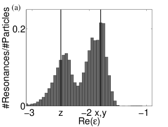
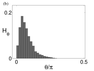
Figure 8: Location of the resonances ((a): all) and orientation of the induced dipole moments ((b): largest only) for the perturbed spheroids. The vertical lines in (a), labeled by z and x,y, indicates the resonant values for the unperturbed spheroid and an incident field along respective coordinate axes.

In Fig. 8 we present histograms for the location of the resonances and for the orientation of the induced dipoles. Again the resonances are shifted to somewhat bigger values of the permittivity. However, now the angle between the incident field and the induced dipole moment for the biggest resonance is much smaller, and also the distribution of the angle is narrower than in the previous case of the perturbed spheres. This comparison can be roughly quantified by the respective mean values, and the widths of the distributions of the angles. We focus again on the biggest resonances only, and determine the mean value $\overline{\theta}$ of the angle and the interval $I_{\theta}$, centered around the mean value, which contains two-thirds of the resonances. For the case of the sphere this results in $\overline{\theta}=1.04$ and $I_{\theta}=[0.65:1.43]$, whereas $\overline{\theta}=0.23$ and $I_{\theta}=[0.09:0.37]$ for the case of spheroids.

V Conclusion

We have presented a simple-to-implement and efficient numerical scheme for calculating important characteristics for surface modes of sphere-like nanoparticles in the quasistatic limit, based on an expansion of the “inner” and “outer” potentials into spherical harmonics. Although the spherical harmonics do not constitute an orthogonal basis for particles which are not exactly spherical, and therefore encounter problems similar to those connected with the Rayleigh hypothesis when the deviation from an exact sphere becomes too strong, they still remain a useful system of functions, in particular so when the boundary conditions are interpreted in an integral manner, with a physically motivated choice of test functions.

We have validated this scheme against exact solutions for ellipsoids, and against perturbation-theoretical calculations for deformed spheres. These comparisons and also additional intrinsic numerical tests both show that our method is able to yield accurate results for the resonant permittivities and the polariziabilities even when only quite few spherical harmonics are employed, that is, with quite small basis sets.

This high computational efficiency allows to perform statistical studies of large ensembles of randomly perturbed nanoparticles. This ability is indispensable when designing, e.g., plasmonic waveguides from nanoparticles with small, but uncontrolled fabrication-induced shape fluctuations. On the one hand, typical effects of such imperfections on the performance of these devices can be quantified in this manner; on the other, admissible tolerances can be determined. While the specific distribution of shape fluctuations employed for demonstration purposes in our example given in Sec. IV may not be realistic, the key steps of such a large-scale statistical analysis proceed along exactly the same route as outlined there.

Appendix A Structure of the matrices

The structure of the matrices in Eq. (9), i.e. $(M_{1}+\epsilon M_{2})U=M_{3}G$, is:

$${\small M_{1}{=}\left(\begin{array}[]{c c c c| c c c c}a_{0,0,0,0}&a_{1,-1,0,0}&\cdots&a_{N,N,0,0}&b_{0,0,0,0}&b_{1,-1,0,0}&\cdots&b_{N,N,0,0}\\ a_{0,0,1,-1}&a_{1,-1,1,-1}&\cdots&a_{N,N,1,-1}&b_{0,0,1,-1}&b_{1,-1,1,-1}&\cdots&b_{N,N,1,-1}\\ \vdots&\vdots&\ddots&\vdots&\vdots&\vdots&\vdots&\ddots\\ a_{0,0,N,N}&a_{1,-1,N,N}&\cdots&a_{N,N,N,N}&b_{0,0,N,N}&b_{1,-1,N,N}&\cdots&b_{N,N,N,N}\\ \hline\cr 0&0&\cdots&0&d_{0,0,0,0}&d_{1,-1,0,0}&\cdots&d_{N,N,0,0}\\ \vdots&\vdots&\ddots&\vdots&d_{0,0,1,-1}&d_{1,-1,1,-1}&\cdots&d_{N,N,1,-1}\\ \vdots&\vdots&\ddots&\vdots&\vdots&\vdots&\ddots&\vdots\\ 0&0&\cdots&0&d_{0,0,N,N}&d_{1,-1,N,N}&\cdots&d_{N,N,N,N}\end{array}\right)},$$

$$M_{2}=\left(\begin{array}[]{c | c }\bm{0}&\bm{0}\\ \hline\cr(c_{l,m,l^{\prime},m^{\prime}})&\bm{0}\end{array}\right),\qquad M_{3}=\left(\begin{array}[]{c | c }(a_{l,m,l^{\prime},m^{\prime}})&\bm{0}\\ \hline\cr(c_{l,m,l^{\prime},m^{\prime}})&\bm{0}\end{array}\right),$$

where $\bm{0}$ is the $(N+1)^{2}\times(N+1)^{2}$ zero matrix. The coefficients $a_{l,m,l^{\prime},m^{\prime}}$, $\cdots$, $d_{l,m,l^{\prime},m^{\prime}}$ are defined by projections of the boundary conditions (2),(3) onto the modes $r^{l^{\prime}}Y^{m^{\prime}}_{l^{\prime}}$ on the surface of the particle $\partial\Omega$:

$$\begin{split}a_{l,m,l^{\prime},m^{\prime}}&=\int\limits_{\partial\Omega}r(s)^{l+l^{\prime}}Y^{m}_{l}(s)\overline{Y^{m^{\prime}}_{l^{\prime}}(s)}\,\text{d}S\,,\\ b_{l,m,l^{\prime},m^{\prime}}&={-}\int\limits_{\partial\Omega}r(s)^{-(l+1)+l^{\prime}}Y^{m}_{l}(s)\overline{Y^{m^{\prime}}_{l^{\prime}}(s)}\,\text{d}S\,,\\ c_{l,m,l^{\prime},m^{\prime}}&=\int\limits_{\partial\Omega}\partial_{n}\left(r(s)^{l}Y^{m}_{l}(s)\right)r(s)^{l^{\prime}}\overline{Y^{m^{\prime}}_{l^{\prime}}(s)}\,\text{d}S\,,\\ d_{l,m,l^{\prime},m^{\prime}}&=-\int\limits_{\partial\Omega}\partial_{n}\left(r(s)^{-(l+1)}Y^{m}_{l}(s)\right)r^{l^{\prime}}\overline{Y^{m^{\prime}}_{l^{\prime}}(s)}\,\text{d}S\,.\end{split}$$

Thus, for a sphere with radius $1$ the coefficients are: $a_{l,m,l^{\prime},m^{\prime}}=\delta_{ll^{\prime}}\delta_{mm^{\prime}},b_{l,m,l^{\prime},m^{\prime}}=-\delta_{ll^{\prime}}\delta_{mm^{\prime}},$ $c_{l,m,l^{\prime},m^{\prime}}=l\delta_{ll^{\prime}}\delta_{mm^{\prime}},d_{l,m,l^{\prime},m^{\prime}}=(l+1)\delta_{ll^{\prime}}\delta_{mm^{\prime}},$ and so only four block diagonals of the matrix $M_{1}+\epsilon M_{2}$ have nonzero entries. The vectors $U$ and $G$ in the system (9) are defined by the coefficients $\alpha_{l,m}$, $\beta_{l,m}$ and $\gamma_{l,m}$ of the expansion of the potentials (5) and (6) as

$$U=\left(\alpha_{0,0},\alpha_{1,-1},\ldots,\alpha_{N,N},\beta_{0,0},\beta_{1,-1},\ldots,\beta_{N,N}\right)^{t},\ G=\left(\gamma_{0,0},\gamma_{1,-1},\ldots,\gamma_{N,N},0,\ldots,0\right)^{t}.$$

References

- (1) U. Kreibig and A. Vollmer, Optical Properties of Metal Clusters (Springer Series in Material Science vol. 25), edited by U. Gonser, R. M. Osgood, M. B. Panish, and H. Sakaki (Berlin, Springer, 1995).
- (2) C. F. Bohren and D. R. Huffman, Absorption and Scattering of Light by Small Particles (New York, Wiley Science, 1998).
- (3) E. Hao and G. C. Schatz, J. Chem. Phys 120, 357 (2004).
- (4) S. Nie and S. Emory, Science 275, 5303 (1997).
- (5) K. Kneipp, Y. Wang, H. Kneipp, L. T. Perelman, I. Itzkan, R. R. Dasari, and M. S. Feld, Phys. Rev. Lett. 78, 1667 (1997).
- (6) S. A. Maier and H. Atwater,J.Appl. Phys. 98, 01101 (2005).
- (7) E. Ozbay, Science 311, 189 (2006).
- (8) M. L. Brongersma, J. W. Hartman, and H. A. Atwater, Phys. Rev. B 62, R16356 (2000).
- (9) S. A. Maier, P. G. Kik, H. A. Atwater, S. Meltzer, E. Harel, B. E. Koel, and A. A. G. Requicha, Nat. Mater. 2, 229 (2003).
- (10) T. Wriedt, Part. Part. Syst. Charact. 15, 67, (1997).
- (11) F. M. Kahnert, JQSRT 79–80, 775, (2003).
- (12) C. Noguez, J. Phys. Chem. C. 111, 3806-3819 (2007
- (13) F. J. García de Abajo and J. Aizpurua, Phys. Rev. B 56, 15873 (1997).
- (14) F. J. García de Abajo and A. Howie, Phys. Rev. B. 65, 115418 (2002).
- (15) U. Hohenester and J. Krenn, Phys. Rev. B 72, 195429 (2005).
- (16) M. I. Mishchenko, L. D. Travis, and A. A. Lacis, Scattering, Absorption, and Emission of Light by Small Particles (Cambridge, Cambridge University Press,2002)
- (17) M. Nieto-Vesperinas, Scattering and Diffraction in Physical Optics (World Scientific, Singapore, 2006).
- (18) A. G. Ramm, J. Phys. A. 35, L357–L361 (2002).
- (19) D. Grieser and F. Rüting, J. Phys. A.: Math. Theor. 72, 135204 (2009).
- (20) M. Galassi et al., GNU Scientific Library Reference Manual (2nd Ed.).
- (21) T. Hahn, Comput. Phys. Commun. 168, 78 (2005).
- (22) E. Anderson et al., LAPACK Users’ Guide 3rd Ed. (Society for Industrial and Applied Mathematics, Philadelphia, PA, 1999).
- (23) D. Grieser, H. Uecker, S.-A. Biehs, O. Huth, F. Rüting, and M. Holthaus, Phys. Rev. B. 80, 245405 (2009).
- (24) N. W. Ashcroft and N. D. Mermin, Solid state physics (Saunders College Publ., Philadelphia, 1976).