New method for calculating shell correction

Abstract

A new method is presented for calculation of the shell correction with the inclusion of the continuum part of the spectrum. The smoothing function used has a finite energy range in contrast to the Gaussian shape of the Strutinski method. The new method is specially useful for light nuclei where the generalized Strutinski procedure can not be applied.

I Introduction

Nuclei being far from the bottom of the stability valley are studied extensively at the experimental facilities with radioactive beams. One of the fruit of these type of research is the production of the light exotic nuclei. Let us refer to e.g. a recently identified new double magic nucleus the ${}^{24}O$ [kan09] at the neutron drip line. The exact location of the particle drip lines limits the region for these studies and it is intensively investigated both by experimental and theoretical methods. Theoretical prediction of the drip lines is based on mass (binding energy) calculations since particle separation energies can be easily deduced.

There are two important theoretical frameworks for global mass calculations. Microscopic HF or HFB calculations with sophisticated effective density dependent interactions are very successful in this field. In the best HFB mass formula so far atk1 the rms error is 674 keV Lun03 . In earlier HF calculations atk2 ; atk3 this number was somewhat larger, namely 805 $keV$ and 822 $keV$ Lun03 . In order to achieve this improved fit a new parameterization of the effective nucleon-nucleon interaction has been introduced and the pairing interaction was treated differently than in the earlier calculations.

Surprisingly a more simple alternative procedure in the framework of the so called macroscopic microscopic (MM) formalism can compete with the microscopic calculations in the calculation of the binding energies. The rms error in the MM calculation is 676 keV. We may say that the quality of the microscopic and MM methods are the same. Despite the almost identical global fits however the microscopic and MM methods show considerable differences when the neutron drip line is approached Lun03 .

The key quantity of the MM calculations is the shell correction. The concept of the shell correction was suggested long time ago by Strutinski [str67] ; [str68] and it is still in use. E.g. in a recent global mass calculation Bha09 the basic ingredient of the shell correction method the smoothed single particle density is calculated in a semi-classical way by the Wigner–Kirkwood expansion. The other elements of the Strutinski method was not altered.

Since the invention of the shell correction there were several refinements of the original method. Besides the original energy averaging, a smoothing in the particle number space was introduced Ton82 ; Pom04 . Even a combination of the two averaging spaces was considered Dia04 . The particle mean field, the simple harmonic oscillator or Nilsson potential was replaced in the calculations by more realistic phenomenological forms in which the spectrum has a continuum beside the discrete single particle levels. The treatment of the single particle level density due to the continuum was a long standing problem [Ro72] ; [Naz94] but an elegant solution was finally reached Kru98 ; [Ve98] .

A large part of the uncertainty due to the proper choice of the technical parameters of the smoothing method has been removed by introduction of the generalized Strutinski procedure[Ve98] ; [Ve00] , which made it possible to calculate reliable shell correction values for medium and heavy nuclei, where the smoothed level density has a long region with linear energy dependence. As it will be discussed in Sec. IV., for lighter nuclei the length of the linear region is reduced due to the reduction of the number of the occupied shells and the increase of the shell gap. For light nuclei the lower and upper ends of the spectrum distort linearity, therefore the method is not appropriate for light nuclei.

The main goal of this work is to develop a new method which is free from this limitation and is applicable for the whole nuclear chart, even in the vicinity of the two drip lines. We are solving this problem by introducing a finite range smoothing instead of the infinite range Gaussian smoothing used in the Strutinski method.

The paper is organized as follows. In Sec. II. we recapitulate the formalism of the calculation of the shell correction. In Sec. III. we describe the standard Strutinski method with the plateau condition. In Sec. IV. we do the same with the generalized Strutinski procedure, what we want to replace in this work. In Sec. V. we describe the new method with finite range smoothing in details. In Sec. VI we apply the new method for several nuclei and calculate shell corrections for neutrons and protons. Finally in Sec. VII. we end with the main conclusions of the paper.

II Calculation of the binding energy by using the shell correction.

The binding energy of an atomic nucleus composed of $A=N+Z$ nucleons ($N$ neutrons and $Z$ protons) $B(N,Z)$ can be calculated in the microscopic-macroscopic model (MM) as

$$B(N,Z)=E_{macr}(N,Z)+\delta E(N,Z)~{},$$ (1)

where $E_{macr}(N,Z)$ is the binding energy calculated in the macroscopic model (e.g. liquid drop or droplet model) and $\delta E(N,Z)$ is the shell correction. While $E_{macr}(N,Z)$ is a smooth function of the number of nucleons, the shell correction takes care of the shell fluctuations of the binding energy which is missing from the macroscopic model. Shell fluctuations are present in any microscopic model. E.g. the shell correction can be calculated from single particle energies of self-consistent Hartree-Fock and relativistic mean filed calculations [Be03] ; [Re06] . In Ref. [Re06] shell correction calculated on the single particle energies was used to generate a smooth energy from the result of these microscopic calculation and the typical phenomenological parameterization of the microscopically calculated macroscopic energy terms were analyzed.

In the present work we use the simplest i.e. the independent particle shell model to generate the single particle energies in a phenomenological nuclear potential for the sake of simplicity only, since the smoothing procedure could be tested equally well on the result of this simple model. In this model we treat neutrons and protons separately. In this case the shell correction

$$\delta E(N,Z)=\sum_{\tau=\nu,\pi}\delta E_{\tau}(N_{\tau})=\delta E(N)+\delta E(Z)$$ (2)

is the sum of the shell corrections $\delta E_{\tau}(N_{\tau})$ calculated for neutrons: $\tau=\nu$ with $N_{\nu}=N$ and for protons $\tau=\pi$ with $N_{\pi}=Z$ . In what follows we shall discuss the calculation of the shell correction $\delta E_{\tau}(N_{\tau})$ for a sort of nucleons only.

The shell correction can be estimated as the difference of the shell model binding energy $E_{sp}^{\tau}$ and its smoothed counterpart $\tilde{E}^{\tau}$ calculated also in the shell model.

$$\delta E_{\tau}=E_{sp}^{\tau}-\tilde{E}^{\tau}~{}.$$ (3)

Here the shell model binding energy

$$E_{sp}^{\tau}=\sum_{j=1}^{N_{\tau}}E_{j}^{\tau}$$ (4)

is a sum of the single particle energies $E_{j}^{\tau}$ of the lowest energy orbits, from $E_{1}^{\tau}$ until the Fermi-level. In the sum above we can take into account the $n_{i}$-fold degeneracies of the shell model orbits and use only the different single particle energies denoted by $e_{i}^{\tau}$

$$E_{sp}^{\tau}=\sum_{i}n_{i}~{}e_{i}^{\tau}~{}.$$ (5)

The key quantity of the MM model is the smoothed energy $\tilde{E}^{\tau}~{}$ therefore, we have to give a unique definition for calculating it unambiguously. If we have the bound single particle energies: $e_{i}^{\tau}$, the density of the bound nuclear levels is

$$g_{\rm d}^{\tau}(E)=\sum_{i}n_{i}~{}\delta(E-e_{i}^{\tau}).$$ (6)

The particle number as a functions of the energy $E$ of the single nucleon considered is an integral of the level density in Eq.(6), i.e. it is equal to the following step function:

$$n^{\tau}(E)=\int_{-\infty}^{E}g_{\rm d}^{\tau}(e)de=\sum_{i}n_{i}~{}\Theta(E-e_{i}^{\tau})~{},$$ (7)

where $\Theta(x)$ is a Heaviside function of the form:

$$\Theta(x)=\left\{\begin{array}[]{rl}0&\textrm{, if }x~{}<~{}0\\ 1&\textrm{, if }x~{}\geq~{}0~{}.\end{array}\right.$$ (8)

Since in the smoothing procedure we treat neutrons and protons on the same footing, we can drop the $\tau$ index for a moment. ( We shell include it later again when it is needed to avoid ambiguity.) We can calculate the smoothed level density $\tilde{g}(E)$ from the level density in Eq.(6) by folding it with a properly selected smoothing function: $f_{p}(x)$. The smoothing function spreads the energy of a discrete level over a certain energy range characterized by the smoothing range parameter $\gamma$. Therefore, the smoothed level density is

$$\tilde{g}(E)=\frac{1}{\gamma}\int_{-\infty}^{+\infty}g(e)~{}f_{p}\left(\frac{e-E}{\gamma}\right)de~{}.$$ (9)

The smoothing function in Eq.(9) is usually a product of a weight function $w(x)$ and a polynomial $h_{p}(x)$ of degree $p$

$$f_{p}(x)=w(x)~{}h_{p}(x).$$ (10)

The later is called as curvature correction polynomial. Since the smoothing function $f_{p}(x)=f_{p}(-x)$ is an even function of $x$, for an even weight function $w(x)$ the polynomial $h_{p}(x)$ should also be even and the coefficients of the odd terms in it should be equal to zero. Therefore, the curvature correction polynomial has the form:

$$h_{p}(x)=\sum_{i=0,2,...,p}c_{i}x^{i}~{}.$$ (11)

The $c_{i}$ coefficients of the curvature correction polynomial $h_{p}(x)$ are determined from the so called self-consistency condition [Bun72] , which requires that the smoothing should reproduce the original function if it is a polynomial $g_{n}(x)$ with degree $n\leq p+1$:

$$g_{n}(x)=\int_{-\infty}^{+\infty}g_{n}(x^{\prime})~{}f_{p}(x-x^{\prime})dx^{\prime}~{}.$$ (12)

We calculate the smoothed energy by using the smoothed level density in Eq.(9) :

$$\tilde{E}=\int_{-\infty}^{\tilde{\lambda}}\epsilon\,\tilde{g}(\epsilon)d\epsilon~{}.$$ (13)

The smoothed Fermi-level $\tilde{\lambda}$ is calculated from the condition that the number of neutrons and protons, i.e. the particle number is given:

$$N=\int_{-\infty}^{\tilde{\lambda}}\tilde{g}(\epsilon)d\epsilon~{}.$$ (14)

The smoothed Fermi-level $\tilde{\lambda}$ is different from the Fermi-level $\lambda$ because the level density has been modified by the smoothing.

III Standard Strutinski method with plateau condition

Strutinski used a smoothing function with a Gaussian a weight function

$$w(x)=\frac{1}{\sqrt{\pi}}\exp(-x^{2})~{},$$ (15)

and it can be shown that the curvature correction polynomials for a weight function of Gaussian shape are the associated Laguerre-polynomials

$$h_{p}(x)=L_{p/2}^{1/2}(x^{2})~{}.$$ (16)

Therefore, in the standard Strutinski method the smoothing function is

$$f_{p}(x)=\frac{1}{\sqrt{\pi}}\exp(-x^{2})L_{p/2}^{1/2}(x^{2})~{}.$$ (17)

For nuclei lying on the bottom of the stability valley the single particle potential can be approximated by a simple harmonic oscillator (h.o.) form. For a nucleus with mass number $A$ the distance of consecutive shells can be expressed by the well known rule [Mo57]

$$\hbar\Omega_{0}=41~{}A^{-1/3}~{}~{}[MeV]~{}.$$ (18)

Shell structure of this simple h.o. model is modified by the presence of the spin-orbit interaction and also by the non-spherical shape of deformed nuclei but the quantity in Eq.(18) is still serves as a reasonably good measure for the shell structure. An attractive feature of the h.o. potential is that the shell correction $\delta E(\gamma,p)$ as a function of the smoothing range $\gamma$ shows a wide plateau in which the

$$\frac{\partial\delta E(\gamma,p)}{\partial\gamma}=0$$ (19)

plateau condition is fulfilled. More precisely, the fulfillment of the plateau condition is valid if at the same time the values belonging to the plateau are practically independent of the $p$ value used. It was observed that the plateau condition is fulfilled for h.o. potential. Since $\gamma$ and $p$ are technical parameters of the smoothing procedure and they have no physical meaning, it is natural to expect that the definition of the smoothed quantities should not depend strongly on these values. Therefore, the shell correction calculated for the h.o. potential is well defined. This nice feature of the h.o. potential is related to the fact that this potential has only bound states (even at high positive energy values). For potentials which are similar to the harmonic oscillator potential e.g. the Nilsson potential we can always find regions for $\gamma$ where the plateau condition is fulfilled [Bra73] ; [Ro72] . Since these potentials have only bound states (infinitely many) and no continuum the ending of the bound states does not spoil the picture.

IV Generalized Strutinski procedure for spectra with continuum

However a more realistic single particle potential has a discrete spectrum with finite number of bound states $e_{i}<0$ and a continuum of scattering states with $E>0$ energy. The full level density in this case is a sum of the level densities of the discrete states $g_{\rm d}(E)$ and that of the scattering states $g_{\rm c}(E)$ forming the continuum

$$g(E)=g_{\rm d}(E)+g_{\rm c}(E).$$ (20)

Now the smooth level density has to be calculated again with the prescription of Eq.(9). It was realized by Brack and Pauli[Bra73] that for this case the plateau condition can not be satisfied since the $\delta E(\gamma,p)$ curves, what we call plateau curves do not have wide plateaus, where Eq.(19) is fulfilled. They searched for the minima $\delta E(\gamma_{p},p)$ of the plateau curves for each $p$ values and introduced the concept of local plateau condition. At the minima i.e. at $\gamma=\gamma_{p}$ Eq.(19) is certainly satisfied. An additional requirement of the local plateau condition is the approximate $p$-independence of the $\delta E(\gamma_{p},p)$ values, which is satisfied if the variation of the $\delta E(\gamma_{p},p)$ values are small.

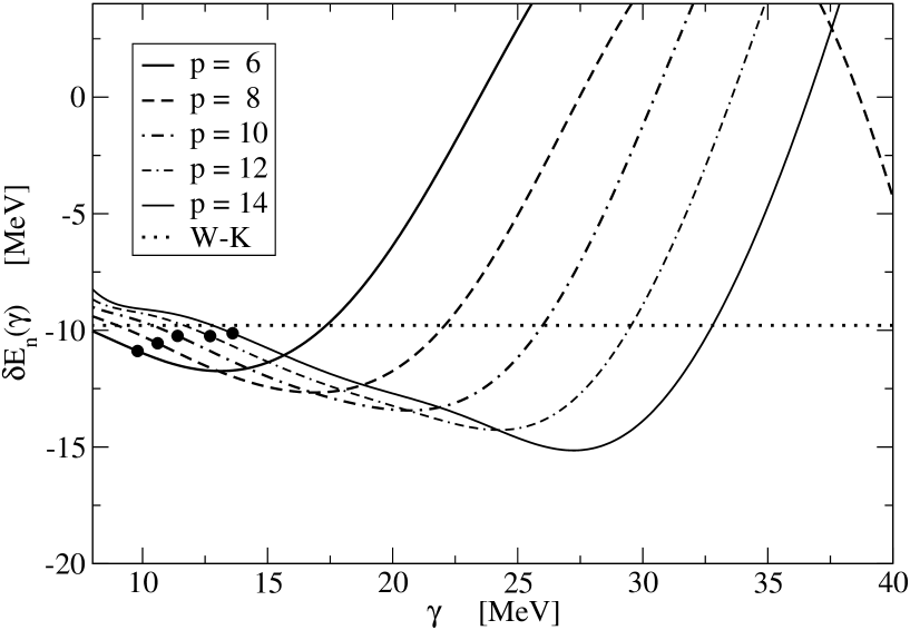
Figure 1: Neutron shell correction $\delta E_{n}(\gamma,p)$ for the nucleus ${}^{146}Gd$ as a function of the smoothing range $\gamma$ calculated for $p=6,..,14$ by using the Gaussian weight function for the smoothing functions $f_{p}$. Filled circles on the different curves denote the $(\gamma_{p},\delta E_{n}(\gamma_{p}))$ points, where $\gamma_{p}$ values belong to the minima of the function in Eq.(21) and the $\delta E_{n}(\gamma_{p},p)$ values are the results of the generalized Strutinski procedure. Dotted horizontal line shows the value of the semi-classical value $\delta E_{sc}=E_{sc}-E_{sp}^{n}$.

It was shown in Ref.[Ve98] that sometimes even the local plateau condition might not be fulfilled and the smoothing procedure of the standard Strutinski method might not able to furnish us with well defined smoothed energy. A typical nucleus for which the local plateau condition fails if the continuum part of the spectrum is taken into account is the ${}^{146}Gd$, as one can see in Fig. 1. Although one can find minima for each plateau curves, the shell correction values at these minima vary too much (even an approximate $p$-independence is not hold). Therefore it is not surprising that the $\delta E(\gamma_{p},p)$ values deviate considerably from the semi-classical value.

In order to cure this difficulty in the work [Ve98] a modified plateau condition was suggested. In the modified plateau condition the plateau condition in Eq.(19) is replaced by the requirement that in a certain energy region the smoothed level density should be fitted well by a straight line.

The shell correction $\delta E(\gamma_{p},p)$ for a given $p$ should be calculated with those $\gamma_{p}$ value for which the smoothed level density can be fitted best by a linear function: $y(E)=aE+b$ in a certain energy range: $[e_{l},e_{u}]$. So we should find the minimum of the function in the variable $\gamma$ for each $p$ value

$$\chi^{2}(\gamma,p)=\sum_{i=1}^{n_{u}}\Big{[}{\tilde{g}}(q_{i},\gamma,p)-y(q_{i})\Big{]}^{2}.$$ (21)

Here $q_{i}$ for $i=1,..,n_{u}$ is a mesh of the energy interval $[e_{l},e_{u}]$ used, and $\gamma_{p}$ is the value where the function $\chi^{2}$ has its minimum at a given $p$-value. To get rid of the shell fluctuations the length of the interval has to be larger than the estimated shell gap

$$e_{u}-e_{l}=1.5~{}\hbar\Omega_{o}~{}.$$ (22)

Having selected the proper $\gamma_{p}$ value for a set of $p$ values between $p_{min}=6$ and $p_{max}=14$, the mean value and the variation of the corresponding $\delta E(\gamma_{p},p)$ values have to be calculated as follow:

$$\delta{E}=\frac{2}{(p_{max}-p_{min}+2)}\sum_{p=p_{min},p_{min}+2,...,p_{max}}~{}\delta{E}(\gamma_{p},p)~{},$$ (23)

$$\sigma=\sqrt{\frac{2}{(p_{max}-p_{min}+2)}\sum_{p=p_{min},p_{min}+2,...,p_{max}}~{}(\delta{E}(\gamma_{p},p)-\delta{E})^{2}}~{}.$$ (24)

Since in Ref.[Ve98] this variation was reasonably small for most of the nuclei, the mean in Eq.(23) was used to define the shell correction and the variation in Eq.(24) was considered as an uncertainty of the method. The procedure described above was called as a generalized Strutinski procedure.

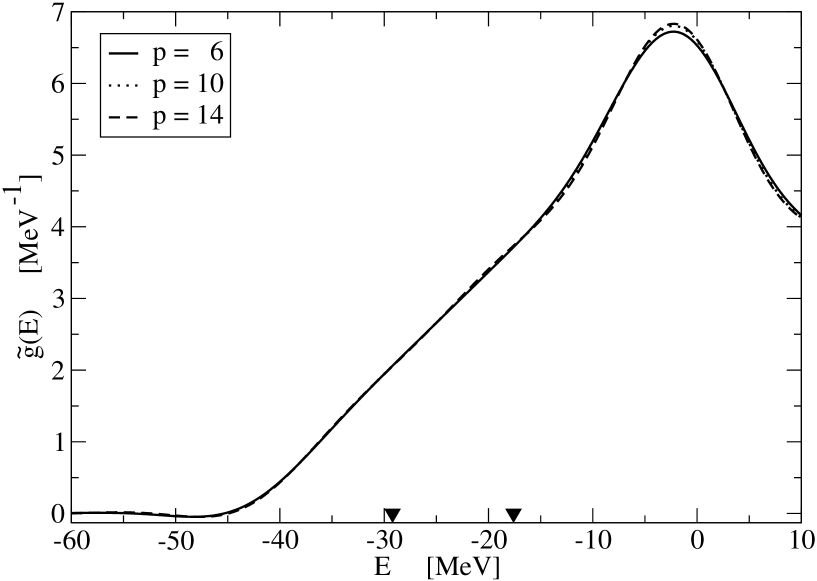
Figure 2: Energy dependence of the smoothed level densities calculated in the generalized Strutinski procedure for $p=6,10,14$ by using a Gaussian weight function for the smoothing functions $f_{p}$ for the nucleus ${}^{146}Gd$ . The lower and upper ends of the interval $[e_{l},e_{u}]$ in which the condition of the best linear fit is applied are shown by triangles on the $E-$ axis.

In order to illustrate the use of the modified plateau condition we present the smoothed level densities for the ${}^{146}Gd$ nucleus in Fig. 2. The lower and upper ends of the energy interval in which the best linear fit of the $\tilde{g}(E)$ is required are shown by filled triangles on the $E$-axis. Practically no $p$-dependence of the $\tilde{g}(E)$ curves can be observed in the $[e_{l},e_{u}]$ interval where $\tilde{g}(E)$ is apparently behaves as a linear function of $E$. Some $p$-dependence can only observed at around $E\approx-10$ MeV being a bit above the $\tilde{\lambda}$ value and at higher energy in the $E=0$ MeV region which has no influence on the shell correction. The large bump of the smoothed level density around $E=0$ MeV is the effect of the higher end of the spectrum. In the positive part of the spectrum only a few neutron resonance contribute to the level density and their effect is smoothed by the smoothing parameters which are the abscissas of the filled circles in Fig.1. These $\gamma_{p}$ values are between $10-15$ MeV, therefore the end effect is spread well below the threshold. The effect of the lower end is less pronounced but can be seen at $E<-35$ MeV. Here the derivative of $\tilde{g}(E)$ with respect to $E$ changes and at $E<-45$ MeV $\tilde{g}(E)$ goes below zero for a while. The main feature of the $\tilde{g}(E)$ is that the linearity required in Eq.(1) holds only in a certain distance from the lower and upper ends of the spectrum.

In Fig.1 the filled circles on the different $p$ curves show the $(\gamma_{p},\delta E_{n}(\gamma_{p},p))$ points where the $\gamma_{p}$ values are those where the function in Eq.(21) has its minimum. One can see from the circles that these shell correction values have much smaller variation ($\sigma$) than the shell correction values at the minima of the curves. Moreover the mean of the $\delta E_{n}(\gamma_{p},p)$ values denoted by circles is in good agreement with the dotted line showing the semi-classical value. In the work [Ve98] it was found that this situation is quite typical and the generalized Strutinski procedure gave similar values to the result of the semi-classical averaging based on the Wigner–Kirkwood expansion [Bra73] ; [Bha71] ; [Jen73] ; [Jen75] ; [Jen75a] ; [Jen75b] ; [Bra97] in those cases in which the later could be applied. Moreover the generalized Strutinski procedure gave similar results to that of the standard one for all cases where the plateau condition is fulfilled. But it gave a well defined value for the smoothed energy even in cases like ${}^{146}Gd$ where we can not really speak about plateau.

It turned out only later, in the work [Ve00] where the generalized Strutinski procedure was used for deformed nuclei, that the function in Eq.(21) might have more than one minimum in $\gamma$. It was concluded in that the minimum at the smaller $\gamma$ value should be selected.

An uncertainty of the generalized Strutinski smoothing procedure is that the results are slightly depend on the position of the $[e_{l},e_{u}]$ energy interval used. For medium and heavy nuclei the uncertainty of the generalized Strutinski procedure was always below $250$ keV. To get this small variation, the energy interval $[e_{l},e_{u}]$ was adjusted to the smoothed Fermi-level, and the upper end of the energy interval was $e_{u}=\tilde{\lambda}-\hbar\Omega_{0}$. If the interval was shifted up to have $e_{u}=\tilde{\lambda}$ and the length was kept the same as in Eq.(22) a variation of the shell correction by around 400 keV was observed. This uncertainty was still reasonably small and it was comparable to the typical deviation from the semi-classical result.

The dependence on the position of the interval become stronger for light nuclei. If the mass number $A$ is reduced, the distance of the shells estimated in Eq.(18) increases and the length of the interval in Eq.(22) also increases. We should use larger and larger $\gamma$ values for smoothing the shell fluctuations. On the other hand the region in which $\tilde{g}(E)$ is linear becomes shorter and shorter because the effect of the lower end shifts higher and that of the higher end shifts lower. Therefore for small $A$ there is not enough space where the required linear region could develop. The linearity of $\tilde{g}(E)$ function is spoiled by the end effects. This explains why the generalized Strutinski procedure breaks down for light nuclei.

Therefore, in this work our goal is to find a new smoothing procedure which is less sensitive to the end effects, but it still keeps the advantages of the generalized Strutinski procedure i.e. the shell correction is practically independent of the $p$ values ($\sigma$ is small). An additional requirement is that $\tilde{E}$ resulted by the new procedure should not be too different from the result of the semi-classical procedure (Wigner–Kirkwood method) if the later approach can be applied.

V New smoothing procedure

A disadvantage of the smoothing procedures used so far is that the Gaussian weight function $w(x)$ used has an infinite range, therefore, the effect of an energy $e_{i}$ is smeared to the whole energy axis from $-\infty$ to $\infty$. Therefore, the effect of the lower and upper ends of the spectrum influences the whole region of the smoothed level density and also the shell correction $\delta{E}$. In this work we try to reduce the end effects in these quantities by using weight functions which have only a finite range. One possible candidate for a weight function with finite range is a shape

$$w(x)=\left\{\begin{array}[]{rl}ke^{-\frac{1}{1-x^{2}}}&\textrm{, if }|x|~{}<1\\ 0&\textrm{, if }|x|~{}\geq 1.\end{array}\right.$$ (25)

The value of the normalization constant $k$ should be chosen from the condition that

$$1=\int_{-1}^{+1}w(x)~{}dx~{}.$$ (26)

One advantage of the form in Eq.(25) is that all derivative of that function are continuous at $|x|=1$, so the weight function continues smoothly to the regions where it is equal to zero. The effect of the smoothing with this form is localized to the $x\in[-1,1]$ interval. In order to use the new smoothing function we have to recalculate the curvature correction polynomials $h_{p}(x)$ in Eq.(11) for the new weight function (in Eq.(25)). The recalculated polynomials $h_{p}(x)$ will be different from the one in Eq.(16) and they should satisfy the self-consistency condition in Eq.(12), with the finite-range weight function. As it was shown in Ref.[Bun72] , the coefficients $c_{i}$ of the curvature correction polynomials in Eq.(11) are solutions of the system of linear equations:

$$\sum_{i=0}^{p}c_{i}a_{i+j}=\delta_{j,0}~{}~{}~{}~{}~{}~{}~{}~{}~{}0\leq j\leq p~{},$$ (27)

where the coefficients $a_{l}$ are the integrals:

$$a_{l}=\int_{-1}^{1}w(x)x^{l}~{}dx~{}.$$ (28)

The integration is over the interval where the weight function $w(x)$ is different from zero.

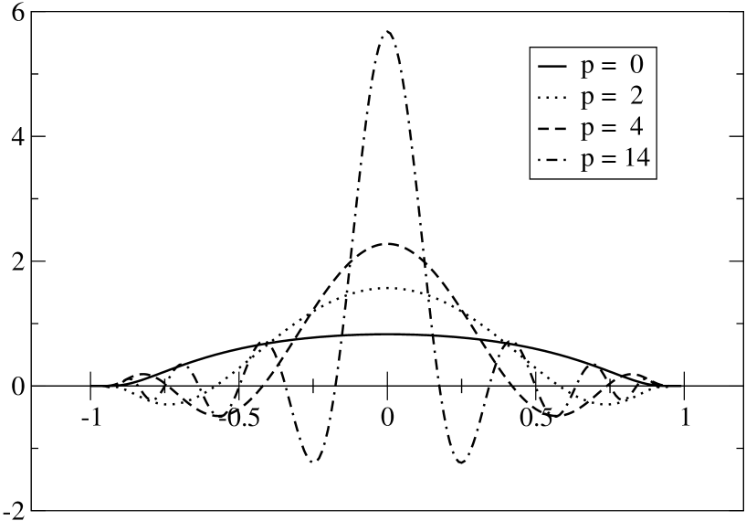
Figure 3: Shapes of the finite range smoothing function $f_{p}(x)$ for $p=0,2,4,14$. Note that $f_{0}(x)=w(x)$.

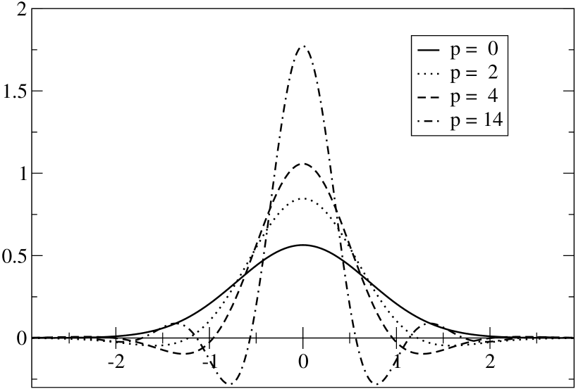
Figure 4: Shapes of the smoothing function $f_{p}(x)$ with Gaussian weight function for $p=0,2,4,14$. Note that the Gaussian weight function is $f_{0}(x)=w(x)$.

We present the coefficients $c_{i}$ for the $p\in\{0,2,4,6\}$ values in Table 1 for illustration purposes. In Fig. 3. we present the shape of the smoothing function $f_{p}(x)$ for a few p values and the finite range weight function in Eq.(25) $w(x)=f_{0}(x)$. In order to show the difference to the standard Gaussian case, we present the similar curves with the Gaussian weight function in Fig.4. For both weight functions for $p>0$ the curvature correction polynomials $h_{p}(x)$ have $p=2m$ zeroes:

$$h_{p}(x_{j}^{(p)})=0,\quad j=\pm 1,...,\pm m,\quad x_{-j}=-x_{j}~{}.$$ (29)

One can observe the positions of the roots $x_{j}^{(p)}$ of the Eq.(29) in Fig. 3 and Fig.4. For a fixed $p$ value it is convenient to arrange the positive roots of Eq.(29) so that they form a monotonous series:

$$0<x_{1}^{(p)}<x_{2}^{(p)}<...<x_{m}^{(p)}~{}.$$ (30)

In the smoothing function $f_{p}(x)$ in Eq.(10) the most important part of the smoothing is produced by the central region in $h_{p}(x)$: $x\in[-x_{1}^{(p)},x_{1}^{(p)}]$, determined by the first root $x_{1}^{(p)}$ . One can see in the figures that for $p>0$ values $x_{1}^{(p+2)}<x_{1}^{(p)}$ i.e. the value of $x_{1}^{(p)}$ decreases when $p$ increases.

The finite range smoothing has the advantage that the effect of a certain single particle energy $e_{i}$ vanishes beyond the interval $E\in[e_{i}-\gamma,e_{i}+\gamma]$. Therefore, the smoothed level density becomes exactly zero for energies lying below $(e_{1}-\gamma)$, while the Gaussian oscillates around zero. This oscillation character appears at any value of the smoothing parameter.

If we go to higher $E$-values, we can smooth the oscillatory character of the $\tilde{g}(E)$ if we use large enough $\gamma$ values in the smoothing function with Gaussian weight function. This is not the case however, if we smooth with finite range weight function, where some undulation in $\tilde{g}(E)$ remains even if we use large smoothing range parameters. Therefore, it can not be well approximated by a straight line as it was in the generalized Strutinski procedure.

This seems to be an important difference between the smoothed level densities calculated by using Gaussian or finite range smoothings.

We calculate the smoothed energy in Eq. (13) by using the finite range smoothing functions, for a range of $\gamma\in[\gamma_{min},\gamma_{max}]$ and $p\in\{p_{min},p_{min}+2,...,p_{max}\}$ values. This allows us to study the plateau curves. For $p=0$ the plateau curve is an monotonously increasing function, therefore, neither the plateau condition in Eq.(19) nor the local plateau condition can be applied. (There is no $\gamma$ value where the derivative is zero.) This result show the necessity of using curvature correction polynomials.

For $p>0$ plateau curves have minima (and maxima) where the plateau condition in Eq.(19) is fulfilled locally. However the plateau curves might have several minima and we have to find the proper one among those minima. A necessary condition of the smoothing is that the smoothed level density should not reflect the shell structure of the single particle levels. Therefore, in the smoothing procedure we have to start searching for the minimum of $\delta{E}(\gamma,p)$ from a ($p$-dependent) $\gamma_{min}$ value with which the shell structure has already disappeared.

The most important characteristics of the single particle spectrum is the largest gap between the occupied levels. Therefore, we have to determine the largest distance between the consecutive occupied levels of the $N$ particles (shell gap)

$$G=\max\Big{\{}(e_{i+1}-e_{i})\Big{\}}~{}.$$ (31)

This $G$ value is a more accurate measure of the shell structure of the single particle energies than the $\hbar\Omega_{0}$ in Eq.(18). In order to estimate a reasonable $\gamma_{min}$ value, we have to determine the effective width of the smoothing function with a given $p$. The effective width corresponds to the central peak of $h_{p}(x)$ in the interval $x\in[-x_{1}^{(p)},x_{1}^{(p)}]$. Since the effective range of the smoothing function decreases for increasing $p$, therefore, for larger $p$ value one should use larger $\gamma$ values for having the same smoothing effect. In order to compensate this effect, it is worthwhile to introduce a renormalized smoothing range as follows:

$$\Gamma_{p}=x_{1}^{(p)}\gamma_{p}~{},$$ (32)

in which the $p$ dependence of the smoothing is considerably reduced.

In order to smooth the fluctuations due to the major shells this $\Gamma_{p}$ range should be larger than the shell gap $\Gamma_{p}>G$. To achieve this we introduce a factor $F>1$, and calculate a minimal value for the renormalized range $\Gamma_{p,min}=FG$. (We observed that the optimal value for the factor $F$ is $F=1.5-2$ for light and $F=2.5-3.5$ for heavier nuclei.) Having fixed this minimum we search for the first minimum of $\delta{E}(\gamma,p)$ for

$$\gamma\geq\gamma_{p,min}=\frac{FG}{x_{1}^{(p)}}.$$ (33)

This criteria serves as a guide to select the proper minimum of the plateau curve $\delta{E}(\gamma_{p},p)$. For most nuclei the plateau curves have multiple minima at $\gamma_{p,1}<\gamma_{p,2}<,..,<\gamma_{p,l}$. The number of minima $l$ generally increases when $p$ increases. We observed that for $p=2$ we have at most two minima, i.e. $l=1$ or $l=2$ and one of them satisfies the following condition:

$$\Gamma_{2,l}=x_{1}^{(2)}\gamma_{2,l}\sim FG~{}.$$ (34)

For higher $p$ values the proper minimum should be close to this value since we reduced the $p$ dependence considerably by using the renormalized smoothing range. Therefore, we have to select the $k$-th minimum, for which $\Gamma_{p,k}=x_{1}^{(p)}\gamma_{p,k}\approx\Gamma_{2,l}$ . If we select the smoothing range according to this criteria then the variation of the corresponding $\delta{E}(\gamma_{p,k},p)$ values will be small.

VI Details of the numerical calculations

We used Saxon-Woods (SW) potential with spin-orbit term. For protons it was complemented by a Coulomb potential of uniformly charged sphere with diffuse edge. (To have this form is necessary for being able to calculate semi-classical results for comparison.) The parameters of the potentials were that of the so called universal potential given in Ref.[dud81] . The depth of the central potential for neutrons ($\tau=\nu$) $t_{3}=1/2$ or for protons ($\tau=\pi$) $t_{3}=-1/2$

$$V_{\tau}(Z,N)=-V\Big{[}1-2\kappa t_{3}\frac{N-Z}{A}\Big{]}~{},$$ (35)

where $\kappa=0.86$, $V=49.6$ MeV. The depth of the spin-orbit potential

$$V_{so}=-\frac{\lambda_{so}V_{\tau}}{4}\Big{(}\frac{\hbar}{2\mu c}\Big{)}^{2}~{},$$ (36)

with the reduced mass $\mu$ of the nucleon and $\lambda_{so}=35(36)$ for neutrons(protons). The diffuseness was $a=a_{so}=a_{C}=0.7$ fm the same for all potential terms. The radius parameters were $r_{0}=1.347$ fm, $r_{0}=r_{C}=1.275$ fm for neutrons and protons, respectively, while for the spin-orbit term $r_{so}=1.31(1.32)$ fm for neutrons(protons). These potential parameters might not be optimal for the individual nuclei but give a good general $N$, $Z$ dependence all over the nuclear chart at least for our purpose for testing our method.

The single particle energies $e_{i}$ of the single particle Hamiltonian were calculated by diagonalizing the matrix of the Hamiltonian in h.o. basis having twenty principal h.o. quanta and maximal orbital angular momentum nine. (An increase of the size of the basis did not change the results.) The same basis was used for diagonalizing the free Hamiltonian (without nuclear potential terms) to get the positive energies $e_{i}^{(0)}$ needed to include the effect of the continuum in the Green’s function method described in Ref.[Ve00] in detail. From the difference of the smoothed level densities of the spectra of the true and the free Hamiltonians the effect of the artificial nucleon gas cancels out and we get the same smoothed continuum level density as we could get by smoothing the continuum level density derived from the derivative of the scattering phase shifts [Ve00] .

In Fig. 5 we show the plateau curves for the ${}^{146}Gd$ nucleus with the finite range smoothing and the result of the Wigner–Kirkwood calculation as a reference. The range of the $p$ values used in the present work was taken to be the same as in Ref. [Ve98] in order to make comparison with those results possible. Using the new method with the finite range smoothing we are able to use the local plateau condition i.e. to choose the $\gamma_{p}$ values where the $\delta{E}(\gamma,p)$ curves have minimum for all the plateau curves shown. The shell correction values at the minima of the curves agree very well (within 500 keV) with the horizontal line representing the result of the semi-classical calculation. Since the $\sigma$ variation of the $\delta{E}(\gamma_{p},p)$ values in Eq. (24) is small the shell correction value calculated from the mean in Eq. (23) is well defined.

In Fig.6 we show an example for the double magic ${}^{132}Sn$ nucleus where the $\sigma$ variation is smaller that 200 keV and the deviation from the semi-classical value $\Delta$ is less than 1 MeV. This is the largest deviation from the cases listed in Table 2. One can observe in both Figs. 5 and 6, that the $\gamma_{p}$ values, where the minima of the $\delta{E}(\gamma_{p},p)$ appear are increasing with increasing $p$ values. This can be compensated to some extent if we use the renormalized smoothing range $\Gamma_{p}$ defined in Eq.(32).

The $\delta{E}(\gamma_{p},p)$ plateau curves are very similar for most nuclei we calculated if we select the values of the first $\gamma_{p}$ minima of the different $p$ curves beyond $\gamma_{p,min}$ in Eq.(33). We identify the shell correction with the mean values of the $\delta{E}(\gamma_{p},p)$ in Eq. (23) and its $\sigma$ variation with the uncertainty of the shell correction.

In Table 2 we show the shell corrections for neutrons and for a set of medium and heavy nuclei resulted by the new smoothing procedure $\delta E_{n}(FR)$, and that of the generalized Strutinski procedure $\delta E_{n}(G)$. Their $\sigma$ variations are in the third and in the fifth columns. In the last two columns we compare their values to that of the semi-classical procedure given in Ref.[Naz94] . The differences from $\delta E_{sc}$ are below $1$ MeV for the new procedure which is a bit better agreement than it is by using the generalized Strutinski procedure. The average of the differences are $0.6$ MeV and $0.8$ MeV for these two procedure, respectively.

In Table 3 we show the similar results for protons, where the average of the differences from the semi-classical results are $0.4$ MeV and $0.6$ MeV for the new procedure and for the generalized Strutinski procedure, respectively. So the new procedure can be applied for protons as well.

These differences are not large neither for neutrons nor for protons. The result of the new procedure is generally closer to the semi-classical result if we approach the drip lines. See e.g. the ${}^{78}Ni$, ${}^{122}Zr$, ${}^{124}Zr$ nuclei for neutrons and the ${}^{180}Pb$ nucleus for proton. Therefore, we believe that the finite range smoothing allows us to approach the drip line closer than we can approach it by using the infinite range Gaussian weight function.

The basic advantage of the new method is however, that the determination of the proper shell correction value is better defined. The values resulted by the new procedure are free from most of the uncertainties of the generalized Strutinski smoothing procedure. E.g. they do not depend on the position of the interval where the linearity of the smoothed level density is required.

The most important advantage of the new procedure is that it can be applied for light nuclei where, as we have discussed in Sec.IV. the generalized Strutinski procedure can not be applied.

The results of the new method for light nuclei are shown in Table 4 for neutrons and in Table 5 for protons. One can see that the agreement with the semi-classical values are as good it was for heavier nuclei. We received specially good agreement for oxygen isotopes even at the neutron drip line.

In Fig.7 we show the neutron plateau curves for the new double magic nucleus ${}^{24}O$ as functions of the renormalized smoothing range parameter $\Gamma_{p}$, for $p=6,8,...,14$. The semi-classical result is the dotted horizontal line. The minima of each curve are denoted by filled circles on the corresponding curves. One can see that the $\delta E_{n}(\Gamma_{p},p)$ values denoted by circles are between -0.9 and -2.3 MeV and their $\Gamma_{p}$ values are quite similar at $\Gamma_{p}\sim 8MeV$. The variation of the $\delta E_{n}(\Gamma_{p},p)$ values are $\sigma\sim 0.5MeV$ and their mean value coincide with the semi-classical value. This is certainly an accident but one can see that the $\Delta$ value is small for the other $O$ isotopes too. Observe also that the positions of the minima of the different $p$ curves in this figure scatter much less in $\Gamma$ ($\sim 15$ %) than the locations of the minima in Fig.6 where the smoothing range $\gamma$ was used ($\sim 90$ %) or in Fig.5 where the smoothing range $\gamma$ was used ($\sim 70$ %).

Therefore, we believe that the finite range smoothing allows us to approach the drip line closer than we can approach it by using the infinite range Gaussian weight function.

VII Conclusion

The new method uses a finite range smoothing function which makes it possible to localize the effect of a single particle state with energy $e_{i}$ to a finite energy range: $[e_{i}-\gamma,e_{i}+\gamma]$. This localization makes possible to extend the region of applicability of the method to closer to the end regions of the spectrum. This helps in calculating shell corrections for slightly bound nuclei lying closer to drip lines and also for lighter nuclei, where the shell gap is large, therefore, larger values of $\gamma$ values are needed to smooth the shell structure out. The new method works equally well for calculating neutron and proton shell corrections.

We introduced a renormalized smoothing range in which the $p$ dependence of the smoothing range was reduced considerably. Using this renormalized range the selection of the proper minimum of the plateau curves was easier.

Therefore, we recommend the use of the new procedure with finite range smoothing first of all for light nuclei, where the generalized Strutinski method can not be applied. We also recommend its use in regions being close to drip lines where the finite range smoothing seems to work somewhat better than the generalized Strutinski method.

VIII Acknowledgement

This work has been supported by the Hungarian OTKA fund No. K72357.

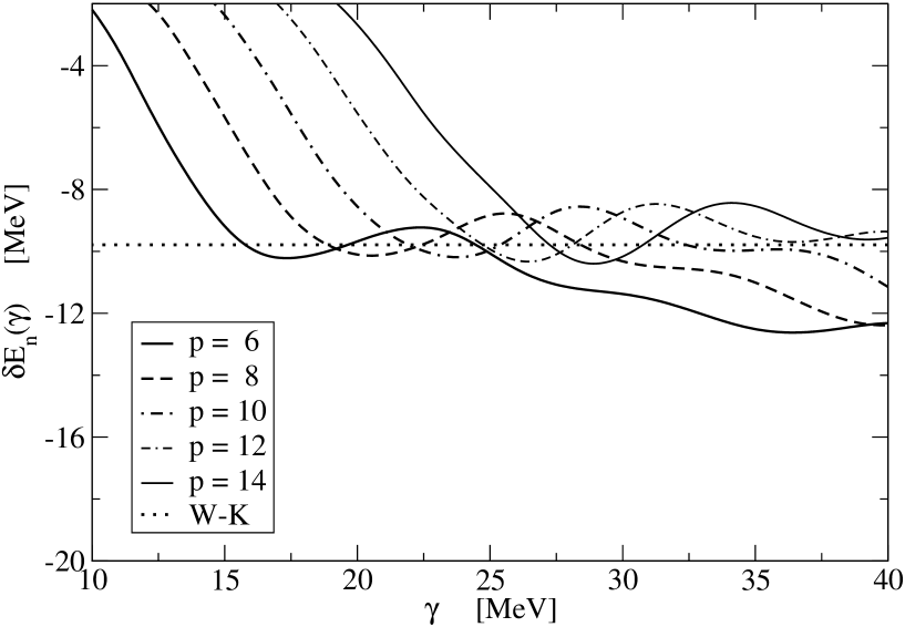
Figure 5: Neutron shell corrections $\delta E_{n}(\gamma,p)$ for the nucleus ${}^{146}Gd$ as a function of the smoothing range $\gamma$ calculated for $p=6,..,14$ by using the finite-range weight function for the smoothing functions $f_{p}$. Dotted horizontal line shows the value of the semi-classical value $\delta E_{sc}=E_{sc}-E_{sp}^{n}$.

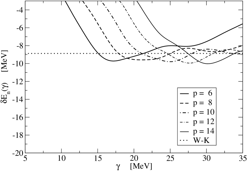
Figure 6: Neutron shell corrections $\delta E_{n}(\gamma,p)$ for the nucleus ${}^{132}Sn$ as a function of the smoothing range $\gamma$ calculated for a set of $p$-values by using the finite-range smoothing function $f_{p}$. Dotted horizontal line shows the value of the semi-classical value $\delta E_{sc}=E_{sc}-E_{sp}^{n}$.

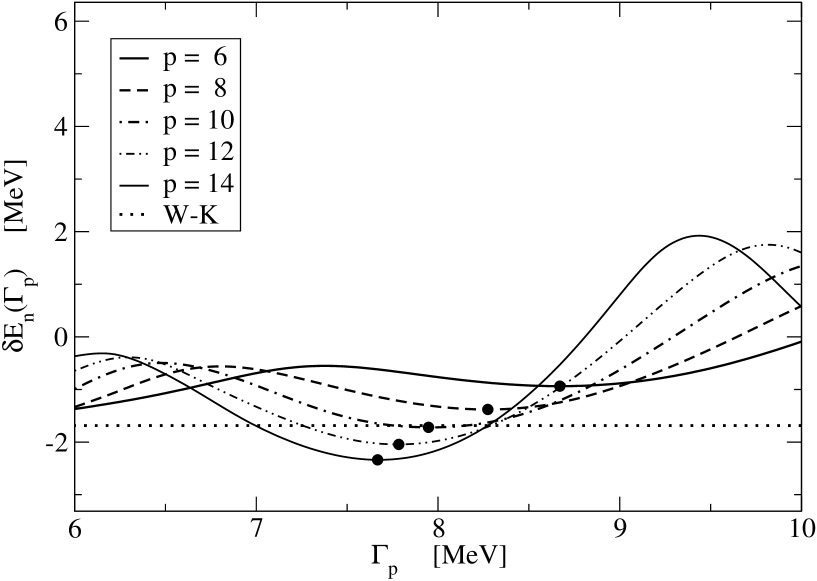
Figure 7: Neutron shell correction $\delta E_{n}(\Gamma_{p})$ for the nucleus ${}^{24}O$ as a function of the renormalized smoothing range $\Gamma_{p}$ calculated for a set of $p$-values by using the finite-range smoothing function $f_{p}$. Dotted horizontal line shows the semi-classical value: $\delta E_{sc}=E_{sc}-E_{sp}^{n}$.

$p$	$c_{0}$	$c_{2}$	$c_{4}$	$c_{6}$
$0$	$1$	$0$	$0$	$0$
$2$	$1.8934$	$-5.6506$	$0$	$0$
$4$	$2.7492$	$-20.62052$	$28.52324$	$0$
$6$	$3.5866$	$-48.45461$	$155.33082$	$-136.79695$

Table 1: Coefficients of the curvature correction polynomials for the lowest $p$ values corresponding to the finite-range weight function in Eq.(25)

Nucleus	$\delta E_{n}(FR)$	$\sigma$	$\delta E_{n}(G)$	$\sigma$	$\delta E_{sc}$	$\Delta_{FR}$	$\Delta_{G}$
$~{}^{68}Ni$	$0.16$	$0.12$	$0.50$	$0.07$	$0.81$	$0.65$	$0.31$
$~{}^{78}Ni$	$-3.59$	$0.07$	$-2.78$	$0.16$	$-4.21$	$0.62$	$1.43$
$~{}^{90}Zr$	$-7.42$	$0.06$	$-7.35$	$0.17$	$-6.82$	$0.60$	$0.53$
$~{}^{122}Zr$	$-5.92$	$0.11$	$-4.52$	$0.15$	$-6.33$	$0.41$	$1.81$
$~{}^{124}Zr$	$-4.12$	$0.12$	$-3.25$	$0.13$	$-4.35$	$0.23$	$1.10$
$~{}^{100}Sn$	$-8.16$	$0.20$	$-6.95$	$0.23$	$-7.50$	$0.66$	$0.55$
$~{}^{132}Sn$	$-9.85$	$0.14$	$-8.58$	$0.10$	$-8.87$	$0.98$	$0.29$
$~{}^{146}Gd$	$-10.26$	$0.07$	$-10.33$	$0.20$	$-9.79$	$0.47$	$0.54$

Table 2: Neutron shell corrections $\delta E_{n}$ and their variations $\sigma$ calculated using the finite range weight function $(FR)$ and the generalized Strutinski procedure $G$ in comparison with the semi-classical shell correction $\delta E_{sc}=E_{sc}-E_{sp}^{n}$ calculated for several nuclei. Their deviations from the semi-classical result $\Delta_{FR}=|\delta E_{sc}-\delta{E}_{n}(FR)|$,   $\Delta_{G}=|\delta E_{sc}-\delta{E}_{n}(G)|$ are also shown. All energies are in MeV units.

Nucleus	$\delta E_{p}(FR)$	$\sigma$	$\delta E_{p}(G)$	$\sigma$	$\delta E_{sc}$	$\Delta_{FR}$	$\Delta_{G}$
$~{}^{90}Zr$	$1.59$	$0.19$	$1.88$	$0.20$	$1.44$	$0.15$	$0.44$
$~{}^{100}Sn$	$-7.47$	$0.064$	$-7.42$	$0.14$	$-7.01$	$0.46$	$0.41$
$~{}^{132}Sn$	$-7.39$	$0.068$	$-6.04$	$0.12$	$-6.64$	$0.75$	$0.60$
$~{}^{146}Gd$	$4.89$	$0.10$	$5.28$	$0.24$	$4.52$	$0.37$	$0.76$
$~{}^{180}Pb$	$-8.94$	$0.15$	$-7.78$	$0.04$	$-8.62$	$0.32$	$0.84$
$~{}^{208}Pb$	$-7.57$	$0.07$	$-6.73$	$0.03$	$-7.29$	$0.28$	$0.56$

Table 3: Proton shell corrections $\delta E_{p}$ and their variations $\sigma$ calculated using the finite range weight function $(FR)$ and the generalized Strutinski procedure $G$ in comparison with the semi-classical shell correction $\delta E_{sc}=E_{sc}-E_{sp}^{n}$ calculated for several nuclei. Their deviations from the semi-classical result $\Delta_{FR}=|\delta E_{sc}-\delta{E}_{p}(FR)|$,   $\Delta_{G}=|\delta E_{sc}-\delta{E}_{p}(G)|$ are also shown. All energies are in MeV units.

Nucleus	$\delta E_{n}$	$\sigma$	$\delta E_{sc}$	$\Delta$
$~{}^{16}O$	$-1.63$	$0.04$	$-1.57$	$0.06$
$~{}^{18}O$	$2.67$	$0.04$	$3.01$	$0.34$
$~{}^{20}O$	$3.25$	$0.24$	$3.11$	$0.14$
$~{}^{22}O$	$0.12$	$0.53$	$0.09$	$0.03$
$~{}^{24}O$	$-1.68$	$0.49$	$-1.69$	$0.01$
$~{}^{20}Ne$	$3.07$	$0.56$	$3.01$	$0.06$
$~{}^{40}Ca$	$-1.77$	$0.35$	$-0.66$	$0.97$
$~{}^{48}Ca$	$-2.91$	$0.24$	$-2.59$	$0.32$

Table 4: Shell correction $\delta E_{n}$, the variation $\sigma$ in Eq.(24) and the semi-classical shell correction $\delta E_{sc}=E_{sc}-E_{sp}^{n}$ calculated for several nuclei. The deviations $\Delta=|E_{sc}-\tilde{E}|$ are also shown. All energies are in MeV units.

Nucleus	$\delta E_{p}$	$\sigma$	$\delta E_{sc}$	$\Delta$
$~{}^{16}O$	$-1.65$	$0.03$	$-1.44$	$0.21$
$~{}^{18}O$	$-1.65$	$0.10$	$-1.66$	$0.01$
$~{}^{20}O$	$-2.09$	$0.19$	$-1.90$	$0.19$
$~{}^{22}O$	$-2.30$	$0.15$	$-2.14$	$0.16$
$~{}^{24}O$	$-3.10$	$0.66$	$-2.36$	$0.74$
$~{}^{40}Ca$	$-1.62$	$0.12$	$-0.91$	$0.71$
$~{}^{48}Ca$	$-1.70$	$0.19$	$-1.44$	$0.26$
$~{}^{48}Ni$	$-0.80$	$0.36$	$-1.23$	$0.43$
$~{}^{56}Ni$	$-3.67$	$0.29$	$-3.45$	$0.22$

Table 5: Shell correction $\delta E_{p}$, the variation $\sigma$ in Eq.(24) and the semi-classical shell correction $\delta E_{sc}=E_{sc}-E_{sp}^{p}$ calculated for several nuclei. All energies are in MeV units.

References

- (1) R. Kanungo, et al., Phys. Rev. Lett. 102, 152501 (2009).
- (2) S. Goriely, F. Tondeur, and J. M. Pearson, At. Data Nucl. Data Tables 77, 311 (2001).
- (3) D. Lunney, J.M. Pearson and C. Thibault, Rev. Mod. Phys. 75, 1021 (2003).
- (4) M. Samyn, S. Goriely, P.-H. Heenen, J. M. Pearson, and F. Tondeur, Nucl. Phys A 700, 142 (2002).
- (5) S. Goriely, M. Samyn, P.-H. Heenen, J. M. Pearson, and F. Tondeur, Phys Rev C66, 024326 (2002).
- (6) V. M. Strutinski, Nucl. Phys. A 95, 420 (1967).
- (7) V. M. Strutinski, Nucl. Phys. A 122, 1 (1968).
- (8) A. Bhagwat, X. Vinas, M. Centelles, P. Schuck and R. Wyss, Phys. Rev. C81, 044321 (2010).
- (9) K. Pomorski, Phys. Rev. C70, 044306 (2004).
- (10) F. Tondeur, Nucl. Phys. A383, 32 (1982)
- (11) A. Diaz-Torres, Phys. Lett. B594, 69 (2004)
- (12) C.K. Ross and R.K. Bhaduri, Nucl. Phys. A188, 566 (1972).
- (13) W. Nazarewicz, T. R. Werner, and J. Dobaczewski, Phys. Rev. C50, 2860 (1994).
- (14) A.T. Kruppa, Phys. Lett. B431, 237 (1998).
- (15) T. Vertse, A. T. Kruppa, R. J. Liotta, W. Nazarewicz, N. Sandulescu, T. R. Werner, Phys. Rev. C57, 3089 (1998).
- (16) T. Vertse, A. T. Kruppa, W. Nazarewicz, Phys. Rev. C61, 064317 (2000).
- (17) M. Bender, P.-H. Heenen, and P.-G. Reinhard, Rev. Mod. Phys. 75, 121 (2003).
- (18) P. G. Reinhard, M. Bender, W. Nazarewicz, T. Vertse, Phys. Rev. C73, 014309 (2006).
- (19) G.G. Bunatian, V. M. Kolomietz, and V. M. Strutinsky, Nucl. Phys. A188, 225 (1972).
- (20) S. A. Moszkowski, Handbuch der Physics, Vol. XXXIX, p. 411. Springer-Verlag, Berlin, 1957. A 122, 1 (1968).
- (21) M. Brack and H.C. Pauli, Nucl. Phys. A207, 401 (1973).
- (22) R.K. Bhaduri and C.K. Ross, Phys. Rev. Lett. 27, 606 (1971).
- (23) B.K. Jennings, Nucl. Phys. A207, 538 (1973).
- (24) B.K. Jennings, R.K. Bhaduri, and M. Brack, Phys. Rev. Lett. A34, 228 (1975).
- (25) B.K. Jennings and R.K. Bhaduri, Nucl. Phys. A237, 149 (1975).
- (26) B.K. Jennings, R.K. Bhaduri, and M. Brack, Nucl. Phys. A253, 29 (1975).
- (27) M. Brack and R.K. Bhaduri, Semi-classical Physics (Addison-Wesley, Reading, Mass., 1997).
- (28) J. Dudek, Z. Szymański, and T. R. Werner, Phys. Rev. C23, 920 (1981).
- (29) M. Bolsterli, E.O. Fiset, J.R. Nix, and J.L. Norton, Phys. Rev. C5, 1050 (1972).