PLANAR DIRAC DIFFUSION

Abstract

We present the results of the planar diffusion of a Dirac particle by step and barrier potentials, when the incoming wave impinges at an arbitrary angle with the potential. Except for right-angle incidence this process is characterized by the appearance of spin flip terms. For the step potential, spin flip occurs for both transmitted and reflected waves. However, we find no spin flip in the transmitted barrier result. This is surprising because the barrier result may be derived directly from a two-step calculation. We demonstrate that the spin flip cancellation indeed occurs for each “particle” (wave packet) contribution.

03.65.Pm (pacs).

I. INTRODUCTION

In a previous paper[1], we investigated the one-dimensional phenomena of diffusion of a Dirac particle from step and barrier potentials. One of the first observations made in that work was the simplifying fact that spin flip did not occur for either potential. This result was not limited to the non relativistic limit where it might have been expected. It is however, as we shall show below an exceptional result.

We consider in this paper potentials and particle rays situated in a plane, the $y$-$z$ plane. The potentials are functions of only one variable, i.e. $V=V(z)$, while the incoming particle direction lies in the $y$-$z$ plane with $\theta$ the impact angle with the potential. The outgoing wave momenta, be they reflected, transmitted or those in the barrier region, must of course also lie in the $y$-$z$ plane.

In general, for arbitrary $\theta$, spin flip contributions occur for any given incoming polarization. Only when $\theta=0$, i.e. for right-angle impingement does spin flip completely disappear, and this applies both to the step and barrier potentials. This limit case reproduces exactly our previous one-dimensional results[1].

Our primary objective in this paper is to present the more general planar results, i.e. those for arbitrary $\theta$. In doing so, we observe that spin flip is rigourously absent for the transmitted wave in the case of the barrier potential. This is not a resonance phenomena, for even in the so called “particle” limit, in which infinite transmitted (and reflected) waves occur, no spin flip is found. This limit is that pertaining to an incoming wave packet which is small in $z$ compared to the barrier width ($L$). We shall calculate this particle limit by means of the two step method[2, 3] and explicitly verify the absence of spin flip in transmission. The sum of the infinite individual waves reproduces the plane wave results (maximum interference) including resonance phenomena.

Before passing in the next section to a detailed discussion of our planar diffusion, we wish to recall here that for the one-dimensional Dirac equation three forms of interaction occur with a potential, be it a step or barrier of height $V_{\mbox{\tiny$0$}}$, depending upon the energy of the incoming particle $E$. For $E>V_{\mbox{\tiny$0$}}+m$ diffusion ($\mathcal{D}$), for $V_{\mbox{\tiny$0$}}-m<E<V_{\mbox{\tiny$0$}}+m$ tunneling barrier ($\mathcal{T}$), and for $E<V_{\mbox{\tiny$0$}}-m$ Klein energy zone ($\mathcal{K}$). In the diffusion[1] and Klein[4, 5] cases oscillatory solutions exist everywhere. Whereas the tunneling case[6, 7] is characterized by real exponential solutions in the potential region. The interpretation of the Klein case conventionally involves pair production as an interpretation of the Klein paradox[8]. Only the diffusion case interests us in this paper although most (but not all) formulas can be analytically continued into the other energy zones.

II. GENERAL CONSIDERATIONS

The time independent Dirac planar ($y$-$z$) equation for potential “scattering” is easily reduced to a one-dimensional problem when the potential is only a function of one (say $z$) of the planar variables. Separation of variables results in

$$\Psi(\boldsymbol{r},t)=\psi(z)\,\exp[i(p_{\mbox{\tiny$2$}}y-Et)]\,\,,$$

where $p_{\mbox{\tiny$2$}}$ is the momentum component along the $y$-direction and remains so in all regions of the plane. In free space, $V=0$, $\psi(z)$ satisfies

$$-i\,\alpha_{\mbox{\tiny$3$}}\,\psi^{\prime}(z)+\alpha_{\mbox{\tiny$2$}}\,p_{\mbox{\tiny$2$}}\,\psi(z)+\beta\,m\,\psi(z)=E\,\psi(z)\,\,.$$ (1)

With $p_{\mbox{\tiny$3$}}$ the $z$-component of momentum, we have as one of the explicit solutions (polarized in the z-direction)

$$\psi(z)=[\,1,\,\,0,\,\,p_{\mbox{\tiny$3$}}/(E+m),\,\,ip_{\mbox{\tiny$2$}}/(E+m)\,]^{t}\,\,\exp[ip_{\mbox{\tiny$3$}}z]\,\,,$$

up to an overall normalization factor. We note that $p_{\mbox{\tiny$2$}}/p_{\mbox{\tiny$3$}}=\tan\theta$ and $E=\sqrt{p_{\mbox{\tiny$2$}}^{{}^{2}}+p_{\mbox{\tiny$3$}}^{{}^{2}}+m^{\mbox{\tiny$2$}}}$. Throughout this paper we consider the incoming particle (travelling from negative z) polarized as above, but our results will be indifferent to the specific choice of polarization and indeed will be expressed in terms of spin conserving and spin flip.

For the region in which $V(z)=V_{\mbox{\tiny$0$}}$, we must make the following modifications (translation)

$$E\rightarrow E-V_{\mbox{\tiny$0$}}\,\,\,,\,\,\,\,\,p_{\mbox{\tiny$2$}}\rightarrow p_{\mbox{\tiny$2$}}\,\,\,,\,\,\,\,\,p_{\mbox{\tiny$3$}}\rightarrow q_{\mbox{\tiny$3$}}\,\,,$$

with $(E-V_{\mbox{\tiny$0$}})^{{}^{2}}=p_{\mbox{\tiny$2$}}^{\mbox{\tiny$2$}}+q_{\mbox{\tiny$3$}}^{\mbox{\tiny$2$}}+m^{\mbox{\tiny$2$}}$. The existence of a non zero value for $p_{\mbox{\tiny$2$}}$ modifies our spinors when compared to our previous one-dimensional calculations, and hence our diffusion results[1]. It also complicates the kinematic conditions for being in one of the zones $\mathcal{D}$, $\mathcal{T}$ and $\mathcal{K}$. The simplest way to see this is to define a new mass $m_{*}$,

$$m_{*}=\sqrt{p_{\mbox{\tiny$2$}}^{\mbox{\tiny$2$}}+m^{\mbox{\tiny$2$}}}=\sqrt{E^{{}^{2}}\sin^{\mbox{\tiny$2$}}\theta+m^{\mbox{\tiny$2$}}\cos^{\mbox{\tiny$2$}}\theta}\,\,.$$ (2)

Then, the one-dimensional energy zones are simply generalized to

$$\begin{array}[]{cclcccl}(\mathcal{D})&~{}:{}{}{}{}{}&&&E&>&V_{\mbox{\tiny$0$}}+m_{*}\,\,,\\ (\mathcal{T})&~{}:{}{}{}{}{}&V_{\mbox{\tiny$0$}}-m_{*}&<&E&<&V_{\mbox{\tiny$0$}}+m_{*}\,\,,\\ (\mathcal{K})&~{}:{}{}{}{}{}&V_{\mbox{\tiny$0$}}-m_{*}&>&E&.&\end{array}$$

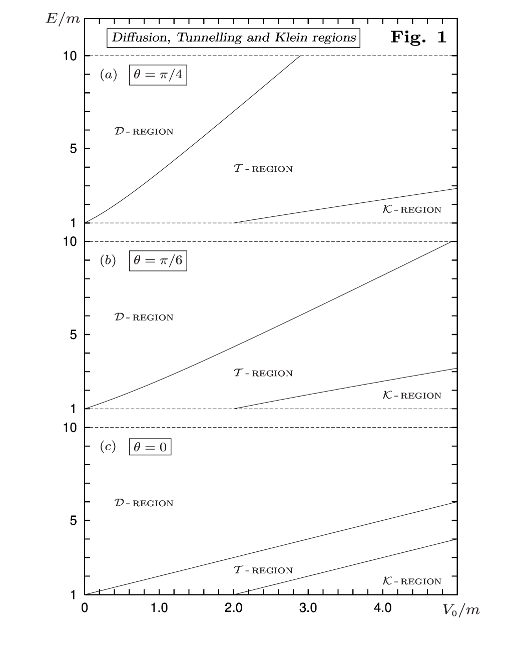
Figure 1: The separate kinematic zones for three choices of incoming angle as a function of potential height. Case (c) corresponds to the one-dimensional plot.

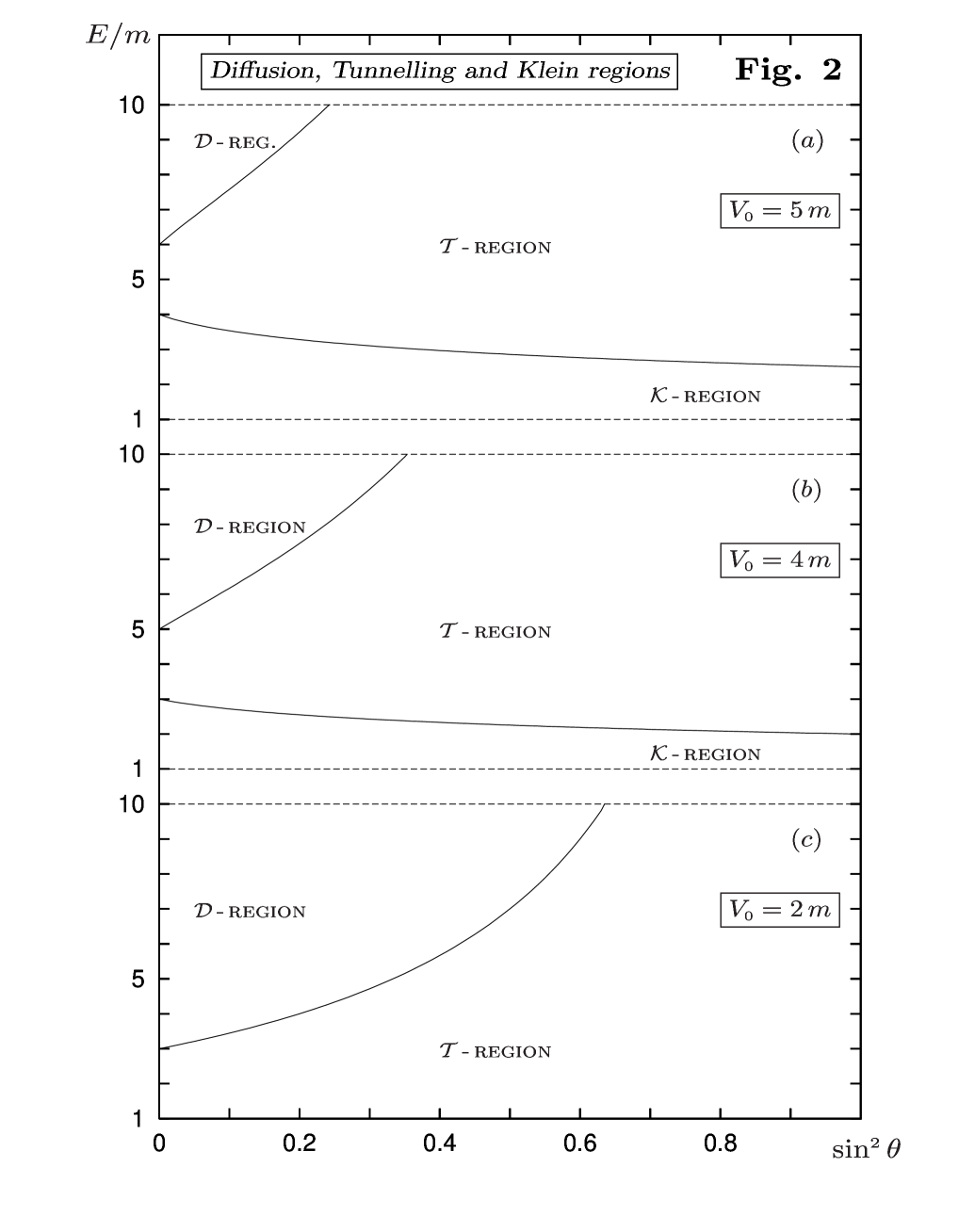
Figure 2: The angular dependence separated into kinematic zones for three choices of potential. Case (c) is the limit case (highest potential) for which there is no Klein zone.

In Figs. (1) and (2), we plot the separation of the various zones by fixing respectively the incident angle $\theta$ and the potential $V_{\mbox{\tiny$0$}}$. The Klein zone is absent for $V_{\mbox{\tiny$0$}}<2m$, see Fig. (2). The plots in Fig. (2) also show that for a given energy $E$, we may transit for high $E$ from $\mathcal{D}$ to $\mathcal{T}$ or for low $E$ from $\mathcal{K}$ to $\mathcal{T}$ by varying the incidence angle $\theta$. For $V_{\mbox{\tiny$0$}}-m<E<V_{\mbox{\tiny$0$}}+m$, only the $\mathcal{T}$ zone exists independent of $\theta$. We note that by varying $\theta$, we can never pass through all three zones. We also note that the one-dimensional kinematics are simply given by the energy points on the axis $\sin^{\mbox{\tiny$2$}}\theta=0$ in Fig. (2).

The Dirac equation, being of first order in the spatial derivatives, implies that continuity equations are applied only to the field. However, this provides four equations, one for each component of the spinors involved. The “small” components correspond in the non relativistic (NR) limit to the continuity of the spatial derivative of the NR field. The remaining doubling of continuity equations (compared to the Schrödinger equation) is exactly what is needed to determine both the spin conserving and spin flip contributions.

In the next section, we apply the continuity condition to the step at $z=0$ for waves coming from either direction (needed in the two-step procedure) and at $z=L$. Below, we sketch the side view for the step calculations of planar diffusion:

In these figures, we list the contributing reflection ($R$) and transmission ($T$) amplitudes. The $\pm$ subscript distinguish an up step from a down step while the tilde represents reflection and transmission for an incoming wave from the right. The prime terms correspond to spin flip amplitudes. In the next section, we also give the results of the continuity equations for the barrier.

III. PLANE WAVE RESULTS

Consider the step potential defined by

$$V(z)=\left\{\,0\,\,\,\mbox{for}\,\,z<0\,\,,\,\,\,V_{\mbox{\tiny$0$}}\,\,\,\mbox{for}\,\,z>0\,\right\}\,\,,$$

with $V_{\mbox{\tiny$0$}}>0$ and with an incoming plane wave from the left (see the step A) with a definite polarization (spin along the $z$-direction). The spinor continuity equations are

$$\left(\,\begin{array}[]{c}E+m\\ 0\\ p_{\mbox{\tiny$3$}}\\ i\,p_{\mbox{\tiny$2$}}\end{array}\,\right)\,\exp[\,ip_{\mbox{\tiny$3$}}z\,]+\left[\,R_{+}(0)\,\left(\,\begin{array}[]{c}E+m\\ 0\\ -p_{\mbox{\tiny$3$}}\\ ip_{\mbox{\tiny$2$}}\end{array}\,\right)+R^{\prime}_{+}(0)\,\left(\,\begin{array}[]{c}0\\ E+m\\ -ip_{\mbox{\tiny$2$}}\\ p_{\mbox{\tiny$3$}}\end{array}\,\right)\,\right]\,\exp[\,-\,ip_{\mbox{\tiny$3$}}z\,]$$ (15)

$$=\frac{E+m}{E-V_{\mbox{\tiny$0$}}+m}\,\,\left[\,T_{+}(0)\,\left(\,\begin{array}[]{c}E-V_{\mbox{\tiny$0$}}+m\\ 0\\ q_{\mbox{\tiny$3$}}\\ i\,q_{\mbox{\tiny$2$}}\end{array}\,\right)+T^{\prime}_{+}(0)\,\left(\,\begin{array}[]{c}0\\ E-V_{\mbox{\tiny$0$}}+m\\ -i\,q_{\mbox{\tiny$2$}}\\ -q_{\mbox{\tiny$3$}}\end{array}\,\right)\,\right]\,\exp[\,iq_{\mbox{\tiny$3$}}z\,]\,\,.$$ (24)

These matrix equations can be rewritten as

$$\left[\begin{array}[]{c}(E+m)\,[1+R_{+}(0)]\\ (E+m)\,R^{\prime}_{+}(0)\\ p_{\mbox{\tiny$3$}}[1-R_{+}(0)]-ip_{\mbox{\tiny$2$}}R^{\prime}_{+}(0)\\ ip_{\mbox{\tiny$2$}}[1+R_{+}(0)]+p_{\mbox{\tiny$3$}}R^{\prime}_{+}(0)\end{array}\right]=\,\frac{E+m}{E-V_{\mbox{\tiny$0$}}+m}\,\,\left[\begin{array}[]{c}(E-V_{\mbox{\tiny$0$}}+m)\,T_{+}(0)\\ (E-V_{\mbox{\tiny$0$}}+m)\,T^{\prime}_{+}(0)\\ q_{\mbox{\tiny$3$}}T_{+}(0)-iq_{\mbox{\tiny$2$}}T^{\prime}_{+}(0)\\ iq_{\mbox{\tiny$2$}}T_{+}(0)-q_{\mbox{\tiny$3$}}T^{\prime}_{+}(0)\end{array}\right]$$

Solution of which yields

$$R_{+}(0) = \frac{(p_{\mbox{\tiny$2$}}^{\mbox{\tiny$2$}}+m^{\mbox{\tiny$2$}}+mE)\,V_{\mbox{\tiny$0$}}}{(E+m)(p_{\mbox{\tiny$3$}}^{\mbox{\tiny$2$}}+p_{\mbox{\tiny$3$}}q_{\mbox{\tiny$3$}}-V_{\mbox{\tiny$0$}}E)}\,\,,$$

$$T_{+}(0) = \frac{p_{\mbox{\tiny$3$}}^{\mbox{\tiny$2$}}(E-V_{\mbox{\tiny$0$}}+m)+p_{\mbox{\tiny$3$}}q_{\mbox{\tiny$3$}}(E+m)}{(E+m)(p_{\mbox{\tiny$3$}}^{\mbox{\tiny$2$}}+p_{\mbox{\tiny$3$}}q_{\mbox{\tiny$3$}}-V_{\mbox{\tiny$0$}}E)}\,\,,$$

$$R^{\prime}_{+}(0) = i\,\frac{p_{\mbox{\tiny$2$}}p_{\mbox{\tiny$3$}}\,V_{\mbox{\tiny$0$}}}{(E+m)(p_{\mbox{\tiny$3$}}^{\mbox{\tiny$2$}}+p_{\mbox{\tiny$3$}}q_{\mbox{\tiny$3$}}-V_{\mbox{\tiny$0$}}E)}\,\,,$$

$$T^{\prime}_{+}(0) = R^{\prime}_{+}(0)\,\,.$$ (25)

Here, we observe that because the step is situated at $z=0$, the $R_{+}(0)$ and $T_{+}(0)$ amplitudes are real while the $R^{\prime}_{+}(0)$ and $T^{\prime}_{+}(0)$ are imaginary. All four amplitudes exist. If we change the incoming polarization (from spin up to spin down), we find exactly the same solutions, although from a different form of matrix equation. This is a general property and we shall henceforth not repeat this observation.

As a simple check of our results, we note that when $V_{\mbox{\tiny$0$}}\to 0$ only $T_{+}(0)=1$ survives as must be. We also observe that as $p_{\mbox{\tiny$2$}}\to 0$ ($\theta\to 0$) the spin flip terms vanish and this confirms our one-dimensional results. The other two step cases (B and C) can be calculated in the same way and yield the results

$$R_{-}(L) = -\,\frac{[p_{\mbox{\tiny$2$}}^{\mbox{\tiny$2$}}+m^{\mbox{\tiny$2$}}+m(E-V_{\mbox{\tiny$0$}})]\,V_{\mbox{\tiny$0$}}}{(E-V_{\mbox{\tiny$0$}}+m)(p_{\mbox{\tiny$3$}}^{\mbox{\tiny$2$}}+p_{\mbox{\tiny$3$}}q_{\mbox{\tiny$3$}}-V_{\mbox{\tiny$0$}}E)}\,\exp[2iq_{\mbox{\tiny$3$}}L]\,\,,$$

$$T_{-}(L) = \frac{q_{\mbox{\tiny$3$}}^{\mbox{\tiny$2$}}(E+m)+p_{\mbox{\tiny$3$}}q_{\mbox{\tiny$3$}}(E-V_{\mbox{\tiny$0$}}+m)}{(E-V_{\mbox{\tiny$0$}}+m)(p_{\mbox{\tiny$3$}}^{\mbox{\tiny$2$}}+p_{\mbox{\tiny$3$}}q_{\mbox{\tiny$3$}}-V_{\mbox{\tiny$0$}}E)}\,\exp[i(q_{\mbox{\tiny$3$}}-p_{\mbox{\tiny$3$}})L]\,\,,$$

$$R^{\prime}_{-}(L) = -\,i\,\frac{p_{\mbox{\tiny$2$}}q_{\mbox{\tiny$3$}}\,V_{\mbox{\tiny$0$}}}{(E-V_{\mbox{\tiny$0$}}+m)(p_{\mbox{\tiny$3$}}^{\mbox{\tiny$2$}}+p_{\mbox{\tiny$3$}}q_{\mbox{\tiny$3$}}-V_{\mbox{\tiny$0$}}E)}\,\exp[2iq_{\mbox{\tiny$3$}}L]\,\,,$$

$$T^{\prime}_{-}(L) = R^{\prime}_{-}(L)\,\exp[-\,i(q_{\mbox{\tiny$3$}}+p_{\mbox{\tiny$3$}})L]=R^{\prime}_{-}(0)\,\exp[i(q_{\mbox{\tiny$3$}}-p_{\mbox{\tiny$3$}})L]\,\,.$$ (26)

While for right impingement at $z=0$ we obtain,

$$\widetilde{R}_{-}(0)=R_{-}(0)\,\,\,,\,\,\,\,\,\widetilde{T}_{-}(0)=T_{-}(0)\,\,\,,\,\,\,\,\,\widetilde{R}^{\prime}_{-}(0)=-R^{\prime}_{-}(0)\,\,\,,\,\,\,\,\,\widetilde{T}^{\prime}_{-}(0)=\widetilde{R}^{\prime}_{-}(0)\,\,.$$ (27)

Passing now to the barrier, we define the reflection and transmission amplitudes respectively in regions I and III by $R$, $R^{\prime}$, $T$ and $T^{\prime}$, while for region II, that of the potential $V_{\mbox{\tiny$0$}}$, we use $A$, $A^{\prime}$, $B$ and $B^{\prime}$. These are not related in a simple manner to our previous step results. The connection will however be derived in the next section.

The expression for $\psi(z)$ within each region are given below. Region I $(z<0)$:

$$\left(\,\begin{array}[]{c}E+m\\ 0\\ p_{\mbox{\tiny$3$}}\\ i\,p_{\mbox{\tiny$2$}}\end{array}\,\right)\,\exp[\,ip_{\mbox{\tiny$3$}}z\,]+\left\{\,R\,\left(\,\begin{array}[]{c}E+m\\ 0\\ -p_{\mbox{\tiny$3$}}\\ ip_{\mbox{\tiny$2$}}\end{array}\,\right)+R^{\prime}\,\left(\,\begin{array}[]{c}0\\ E+m\\ -ip_{\mbox{\tiny$2$}}\\ p_{\mbox{\tiny$3$}}\end{array}\,\right)\,\right\}\,\exp[\,-\,ip_{\mbox{\tiny$3$}}z\,]\,\,.$$ (28)

Region II $(0<z<L)$:

$$\left\{\,A\,\left(\,\begin{array}[]{c}E-V_{\mbox{\tiny$0$}}+m\\ 0\\ q_{\mbox{\tiny$3$}}\\ i\,q_{\mbox{\tiny$2$}}\end{array}\,\right)+A^{\prime}\,\left(\,\begin{array}[]{c}0\\ E-V_{\mbox{\tiny$0$}}+m\\ -i\,q_{\mbox{\tiny$2$}}\\ -q_{\mbox{\tiny$3$}}\end{array}\,\right)\,\right\}\,\exp[\,iq_{\mbox{\tiny$3$}}z\,]\,\,+$$ (37)

$$\left\{\,B\,\left(\,\begin{array}[]{c}E-V_{\mbox{\tiny$0$}}+m\\ 0\\ -q_{\mbox{\tiny$3$}}\\ i\,q_{\mbox{\tiny$2$}}\end{array}\,\right)+B^{\prime}\,\left(\,\begin{array}[]{c}0\\ E-V_{\mbox{\tiny$0$}}+m\\ -i\,q_{\mbox{\tiny$2$}}\\ q_{\mbox{\tiny$3$}}\end{array}\,\right)\,\right\}\,\exp[\,-iq_{\mbox{\tiny$3$}}z\,]\,\,.$$ (46)

Region III $(z>L)$:

$$\left\{\,T\,\left(\,\begin{array}[]{c}E+m\\ 0\\ p_{\mbox{\tiny$3$}}\\ i\,p_{\mbox{\tiny$2$}}\end{array}\,\right)+T^{\prime}\,\left(\,\begin{array}[]{c}0\\ E+m\\ -ip_{\mbox{\tiny$2$}}\\ -p_{\mbox{\tiny$3$}}\end{array}\,\right)\,\right\}\,\exp[\,ip_{\mbox{\tiny$3$}}z\,]\,\,.$$ (47)

In the above expressions factors such as $1/(E+m)$ and $1/(E-V_{\mbox{\tiny$0$}}+m)$ have been absorbed into the amplitudes for simplification. After elimination of the intermediate $A$, $A^{\prime}$, $B$ and $B^{\prime}$ the coupled continuity equations yield the matrix equation

$$\left[\begin{array}[]{c}(E+m)\,(1+R)\\ (E+m)\,R^{\prime}\\ p_{\mbox{\tiny$3$}}(1-R)-ip_{\mbox{\tiny$2$}}R^{\prime}\\ ip_{\mbox{\tiny$2$}}(1+R)+p_{\mbox{\tiny$3$}}R^{\prime}\end{array}\right]=M\,\left[\begin{array}[]{c}(E+m)\,T\\ \ (E+m)\,T^{\prime}\\ p_{\mbox{\tiny$3$}}T-ip_{\mbox{\tiny$2$}}T^{\prime}\\ ip_{\mbox{\tiny$2$}}T-p_{\mbox{\tiny$3$}}T^{\prime}\end{array}\right]\,\exp[\,ip_{\mbox{\tiny$3$}}L]\,\,,$$

where

$$M=\frac{1}{q_{\mbox{\tiny$3$}}}\,\left[\begin{array}[]{cccc}q_{\mbox{\tiny$3$}}\cos(q_{\mbox{\tiny$3$}}L)&q_{\mbox{\tiny$2$}}\sin(q_{\mbox{\tiny$3$}}L)&-i(E-V_{\mbox{\tiny$0$}}+m)\sin(q_{\mbox{\tiny$3$}}L)&0\\ q_{\mbox{\tiny$2$}}\sin(q_{\mbox{\tiny$3$}}L)&q_{\mbox{\tiny$3$}}\cos(q_{\mbox{\tiny$3$}}L)&0&i(E-V_{\mbox{\tiny$0$}}+m)\sin(q_{\mbox{\tiny$3$}}L)\\ -i(E-V_{\mbox{\tiny$0$}}-m)\sin(q_{\mbox{\tiny$3$}}L)&0&q_{\mbox{\tiny$3$}}\cos(q_{\mbox{\tiny$3$}}L)&q_{\mbox{\tiny$2$}}\sin(q_{\mbox{\tiny$3$}}L)\\ 0&i(E-V_{\mbox{\tiny$0$}}-m)\sin(q_{\mbox{\tiny$3$}}L)&q_{\mbox{\tiny$2$}}\sin(q_{\mbox{\tiny$3$}}L)&q_{\mbox{\tiny$3$}}\cos(q_{\mbox{\tiny$3$}}L)\end{array}\right]\,\,.$$

The solution of these equations are

$$R = -\,i\,\left(m+\frac{p_{\mbox{\tiny$2$}}^{{}^{2}}}{E+m}\right)V_{\mbox{\tiny$0$}}\,\frac{\sin(q_{\mbox{\tiny$3$}}L)}{p_{\mbox{\tiny$3$}}q_{\mbox{\tiny$3$}}\mathcal{F}}\,\,,$$

$$R^{\prime} = \frac{p_{\mbox{\tiny$2$}}p_{\mbox{\tiny$3$}}}{E+m}\,V_{\mbox{\tiny$0$}}\,\frac{\sin(q_{\mbox{\tiny$3$}}L)}{p_{\mbox{\tiny$3$}}q_{\mbox{\tiny$3$}}\mathcal{F}}\,\,,$$

$$T = \frac{\exp(-ip_{\mbox{\tiny$3$}}L)}{\mathcal{F}}\,\,,$$

$$T^{\prime} = 0\,\,,$$ (48)

with

$$\mathcal{F}=\cos(q_{\mbox{\tiny$3$}}L)-\,i\,\frac{p_{\mbox{\tiny$3$}}^{{}^{2}}-EV_{\mbox{\tiny$0$}}}{p_{\mbox{\tiny$3$}}q_{\mbox{\tiny$3$}}}\,\sin(q_{\mbox{\tiny$3$}}L)\,\,.$$

These are the generalized barrier results for a plane wave. They contain the momentum $p_{\mbox{\tiny$2$}}$ indicating a dependence upon incident angle. For $p_{\mbox{\tiny$2$}}=0$, we reproduce the one-dimensional Dirac barrier results published in our previous paper[1]. Spin flip is indeed absent in this limit. However, the surprising feature of the general barrier results is that $T^{\prime}=0$ for all incident angles. This was not expected and seems to contrast with the fact that the equivalent terms $T^{\prime}_{\pm}$ are not identically null for the steps.

In the next section, we perform the two step calculation to redetermine the above expressions, in particular that for $T^{\prime}$. This will confirm the above results and demonstrate that $T^{\prime}=0$ is not a resonance phenomena. On the other hand typical resonance behavior is present in the above expressions. Whenever $\sin(q_{\mbox{\tiny$3$}}L)=0$, i.e. for $q_{\mbox{\tiny$3$}}L=n\pi$ (with $n$ a positive integer) both reflected amplitudes, $R$ and $R^{\prime}$, vanish and the transmitted probability $|T|^{{{}^{2}}}=1$. Plane waves are theoretical abstractions, the above results are in truth good approximations only for barrier widths much smaller than the incoming wave packets widths. In other words high values of $n$ corresponding to large $L$ will not exhibit resonance behavior[1].

IV. TWO STEP CALCULATION

In this section, we recalculate the barrier results using the step results. Specifically, this approach for the barrier is called the two step method and does not directly involve the continuity equations of the previous section. The method uses three step results. In addition to that for the step at $z=L$ impinged upon from the left, it also uses the step results at $z=0$ twice. Once for the initial incoming wave (impingement from the left) and then those for a wave reflected from the end of the barrier with consequent impingement at $z=0$ from the right.

This method of calculation can be used to reproduce the standard barrier results by simply adding the infinite contributions to transmission and reflection yielding the so called (plane) wave limit. By treating each contribution as incoherent with the others we obtain the particle limit. Probabilities are conserved in both limits although the total transmission/reflection probabilities are quite different. The wave limit for example is characterized by resonance phenomena, the particle limit is not. In addition to calculating the individual particle limit probabilities for transmission, it is one of our objectives to control if vanishing spin flip is a resonance phenomena or not.

The incoming wave is polarized. At $z=0$ it encounters the first of the two steps and two contributions proceed (are transmitted) to the right. These are indicated by the spin conserving $T_{+}(0)$ and the spin flip term $T^{\prime}_{+}(0)$. At the second (downward) step at $z=L$ each of these contributions produces two transmitted amplitudes. These four transmitted terms combine into two sums: the spin conserving amplitude,

$$A_{\mbox{\tiny T}}=T_{+}(0)T_{-}(L)+T^{\prime}_{+}(0)T^{\prime}_{-}(L)\,\,,$$ (49)

and a spin flip amplitude,

$$A^{\prime}_{\mbox{\tiny T}}=T_{+}(0)T^{\prime}_{-}(L)+T^{\prime}_{+}(0)T_{-}(L)\,\,.$$ (50)

Now, we can use the step results previously given to observe that

$$A_{\mbox{\tiny T}}=\frac{2\,p_{\mbox{\tiny$3$}}q_{\mbox{\tiny$3$}}}{p_{\mbox{\tiny$3$}}^{\mbox{\tiny$2$}}+p_{\mbox{\tiny$3$}}q_{\mbox{\tiny$3$}}-E\,V_{\mbox{\tiny$0$}}}\,\exp[i\,(q_{\mbox{\tiny$3$}}-p_{\mbox{\tiny$3$}})\,L]\,\,\,\,\,\,\,\mbox{and}\,\,\,\,\,\,\,A^{\prime}_{\mbox{\tiny T}}=0\,\,.$$ (51)

So the first particle spin flip contribution is null. This fact alone does not guarantee that subsequent spin flip contributions are null. For example, the second transmitted contributions contain in addition to the $T$ factors also two $R$ factors corresponding to an additional back and forth passage over the barrier,

$$A_{\mbox{\tiny R}} = R_{-}(L)\widetilde{R}_{-}(0)+R^{\prime}_{-}(L)\widetilde{R}^{\prime}_{-}(0)=\frac{(E^{{}^{2}}-p_{\mbox{\tiny$3$}}^{\mbox{\tiny$2$}})\,V_{\mbox{\tiny$0$}}^{{}^{2}}}{(p_{\mbox{\tiny$3$}}^{\mbox{\tiny$2$}}+p_{\mbox{\tiny$3$}}q_{\mbox{\tiny$3$}}-E\,V_{\mbox{\tiny$0$}})^{{}^{2}}}\,\exp[2\,i\,q_{\mbox{\tiny$3$}}\,L]\,\,,$$ (52)

$$A^{\prime}_{\mbox{\tiny R}} = R_{-}(L)\widetilde{R}^{\prime}_{-}(0)+R^{\prime}_{-}(L)\widetilde{R}_{-}(0)=0\,\,.$$ (53)

The overall second contribution to the spin flip is thus

$$A_{\mbox{\tiny T}}A^{\prime}_{\mbox{\tiny R}}+A^{\prime}_{\mbox{\tiny T}}A_{\mbox{\tiny R}}=0\,\,.$$

All higher spin flip contributions take the form of the the above second contribution multiplied by powers of the spin-conserving double reflection factor $A_{\mbox{\tiny R}}$. Thus, the vanishing of the second spin flip term does indeed imply the vanishing of all the spin flip contributions.

We now calculate the individual spin conserving contributions. The first contribution $A_{\mbox{\tiny T}}$ has already been given (49). The second contribution is

$$A_{\mbox{\tiny T}}A_{\mbox{\tiny R}}+A^{\prime}_{\mbox{\tiny T}}A^{\prime}_{\mbox{\tiny R}}=A_{\mbox{\tiny T}}A_{\mbox{\tiny R}}\,\,.$$

All higher (later emerging) contributions are now obvious. The $n$-th term reads,

$$A_{\mbox{\tiny T}}A^{{}^{n-1}}_{\mbox{\tiny R}}\,\,.$$

In the wave limit these contributions must be added coherently to give a single outgoing transmission amplitude. This may conveniently be written as,

$$\frac{A_{\mbox{\tiny T}}}{1-A_{\mbox{\tiny R}}}\,\,.$$ (54)

After inserting the specific step expressions of the previous section, we reproduce after a little algebra the plane wave result for the barrier transmission,

$$T=\frac{A_{\mbox{\tiny T}}}{1-A_{\mbox{\tiny R}}}=\frac{\exp(-ip_{\mbox{\tiny$3$}}L)}{\mathcal{F}}\,\,.$$ (55)

V. CONCLUSIONS

In the literature one normally encounters one dimensional potential analysis. However, when spin and relativity are relevant one-dimensional analysis may be too limited. For example the absence of spin flip terms for one-dimensional step and barrier diffusion is no longer valid for planar diffusion where an angle of incidence exists. The potentials are still considered functions of a single spatial variable ($z$ in this paper) but the incoming particle have two momentum components. This small modification produces significant differences, specifically the appearance, in general, of spin flip terms and consequent modifications in the non-flip amplitudes. We have demonstrated these facts in this paper. These effects are a direct consequence of the angular dependence of the Dirac spinors.

We have found one notable exception to the above, for which we have no simple explanation, although we believe one must surely exist. This exception is that in the case of the barrier potential there is no spin-flip transmission amplitude. There are always spin-flip terms for the step, be the step rising or dropping , except of course for the one dimensional limit when the potential is met head on. This makes the barrier result all the more unexpected, since we know that the barrier result may be derived from a double-step analysis which uses only the step results.

We have listed in the previous sections all relevant planar diffusion results for the step and barrier. We have also derived the transmission amplitude for the barrier in the ”particle” limit via the two-step method. This demonstrates that the absence of spin-flip for each individual outgoing wave packet, independent of the degree of coherence involved, i.e. it is not a resonance type phenomena.

As a side product, we have described the kinematics of dirac planar scattering and observed that by varying the incidence angle, for a given incoming energy we may transit through two kinematic zones, e.g. from diffusion to or from tunnelling, but never through all three kinematic zones $\mathcal{D}$, $\mathcal{T}$, $\mathcal{K}$. We have in the past referred to these zones as energy zones, but this is correct only for one-dimensional studies. They should instead be referred to as kinematic zones which depend upon both energy and angle of incidence. Energy alone, normally does not determine these zones. These kinematic zones are distinguished by quite distinct physics. In this paper, we have limited our attention to diffusion.

References

• [1] S. De Leo and P. Rotelli, Eur. Phys. J. C 46, 551 (2006).
• [2] A. Anderson, Am. J. Phys. 57, 230-235 (1989).
• [3] A. Bernardini, S. De Leo and P. Rotelli, Mod. Phys. Lett. A 19, 2717-2725 (2004).
• [4] P. Krekora, Q. Su, and R. Grobe, Phys. Rev. Lett. 92, 040406 (2004).
• [5] S. De Leo and P. Rotelli, Phys. Rev. A 73, 042107 (2006).
• [6] V.S. Olkhovsky, E. Recami and J. Jakiel, Phys. Rep. 398, 133 (2004).
• [7] S. De Leo and P. Rotelli, Eur. Phys. J. C 51, 241 (2007).
• [8] O. Klein, Z. Phys. 53, 157-165 (1929).
Refer to caption