Theoretical analysis for critical fluctuations of relaxation trajectory near a saddle-node bifurcation

Abstract

A Langevin equation whose deterministic part undergoes a saddle-node bifurcation is investigated theoretically. It is found that statistical properties of relaxation trajectories in this system exhibit divergent behaviors near a saddle-node bifurcation point in the weak-noise limit, while the final value of the deterministic solution changes discontinuously at the point. A systematic formulation for analyzing a path probability measure is constructed on the basis of a singular perturbation method. In this formulation, the critical nature turns out to originate from the neutrality of exiting time from a saddle-point. The theoretical calculation explains results of numerical simulations.

I introduction

To uncover the nature of fluctuations near a bifurcation point has provided a clue to understanding of singularities observed in a rich variety of phenomena. The most typical example of such studies is the Ginzburg-Landau theory for equilibrium critical phenomena GL . According to this theory, the description of fluctuations in the system that undergoes a pitchfork bifurcation is a starting point for characterizing the Ising universality class of the paramagnetic-ferromagnetic transition. The second example is a theory of collective synchronization in coupled oscillators kuramoto . In this phenomenon, the mechanism of the cooperative oscillation is explored by studying fluctuations near a Hopf bifurcation. The third example is related to a theory of directed percolation, whose universality class is characterized by a transcritical bifurcation with a multiplicative noise Munos . From a viewpoint of bifurcation theory, a pitchfork bifurcation, a Hopf bifurcation, and a transcritical bifurcation are local co-dimension one bifurcations Gucken . Now, the last one in this type of bifurcations is a saddle-node bifurcation.

Mathematically, a saddle-node bifurcation in a differential equation is defined as the appearance of a pair of saddle type fixed point and node type fixed point with respect to change in a system parameter. This bifurcation has been found in many models such as a mean field model of the spinodal transition binder , a model of driven colloidal particles reimann , bio-chemical network models bio3 ; spike ; Tyson ; Ohta_co , a dynamical model associated with a $k$-core percolation problem kcore , and a random-field Ising model rfohta . Theoretically, once it is found that a system undergoes a saddle-node bifurcation, its deterministic behavior near the bifurcation point is immediately derived, as seen in standard textbooks Gucken . As an example, a characteristic time scale exhibits divergent behavior proportional to $\epsilon^{-1/2}$, where $\epsilon$ represents the distance from the bifurcation point.

Now, in a manner similar to the other local co-dimension one bifurcations, it is expected that fluctuations near a saddle-node bifurcation exhibits a singular behavior. Thus far, the singular nature of the fluctuations has not been focused on except for some works 1dimlett ; Ohta_co ; kcore ; rfohta ; reimann ; kubokitahara ; spike , and its theoretical study is still immature compared with much progress in theories of fluctuations near the other bifurcations. However, as we already pointed out 1dimlett ; Ohta_co ; kcore ; rfohta , a stochastic model under a saddle-node bifurcation is regarded as the simplest one of systems that exhibit the coexistence of discontinuous transition and critical fluctuation. Such a coexistence has been observed in the dynamical heterogeneity in glassy systems chi4_allstar1 ; chi4_allstar2 ; silbert_mix ; Toninelli_b ; toninelli ; schwartz ; sellitto . Therefore, a theoretical method for describing fluctuations near a saddle-node bifurcation might be useful for studying wider systems including glassy systems (see Sec. V as a related discussion).

With this background, in the present paper, we analyze a Langevin equation for a quantity $\phi$ in which the deterministic part undergoes a saddle-node bifurcation. Especially, we investigate statistical properties of relaxation behavior near the bifurcation point with small noise intensity $T$. Note that $T$ is proportional to the inverse of the number of elements in cases of many-body systems with an infinite range interaction Ohta_co or defined on a random graph kcore ; rfohta . Then, the fluctuation intensity $\chi_{\rm\phi}(t)$ of relaxation trajectories exhibits a divergent behavior similar to those observed in the dynamical heterogeneity. The aim of this paper is to describe this divergent behavior theoretically.

The main idea in our theoretical analysis is to express a single trajectory in terms of a singular part and the others. Concretely, we focus on the exiting time $\theta$ from a saddle-point and find that $\theta$ exhibits the divergent behavior $\left\langle(\theta-\left\langle\theta\right\rangle)^{2}\right\rangle\simeq T^{-2/3}$ in the limit $T\to 0$ with $\epsilon=0$ fixed and $\left\langle(\theta-\left\langle\theta\right\rangle)^{2}\right\rangle\simeq\epsilon^{-5/2}$ in the limit $\epsilon\to 0$ with $T\ll 1$ fixed. In addition to these divergent behaviors, we derive a statistical distribution of $\theta$, by which $\chi_{\phi}(t)$ is calculated. This idea does not only make the calculation possible, but also provides us an insight for the nature of the divergent fluctuations near a saddle-node bifurcation. That is, the most important quantity that characterizes the fluctuations near a saddle-node bifurcation is the exiting time from the saddle-point.

This paper is organized as follows. In Sec. II, we present a model, and display numerical results on divergent behavior of $\chi_{\phi}(t)$. In Sec. III, on the basis of a simple phenomenological argument, we derive critical exponents characterizing the divergent behavior. We also present the basic idea of our theory. In Sec. IV, by employing a singular perturbation method, we construct a systematic perturbation theory so as to determine the statistical properties of the important quantity, $\theta$. Section V is devoted to concluding remarks.

II model

Let $\phi(t)$ be a time dependent one-component quantity. We study relaxation behavior described by a Langevin equation

$$\partial_{t}\phi=f_{\epsilon}(\phi)+\xi.$$ (1)

Here, $f_{\epsilon}(\phi)$ is assumed to be

$$f_{\epsilon}(\phi)=-\epsilon\phi-\phi(\phi-1)^{2},$$ (2)

where $\epsilon$ is a small parameter. $\xi$ in (1) represents Gaussian white noise that satisfies

$$\left\langle\xi(t)\xi(t^{\prime})\right\rangle=2T\delta(t-t^{\prime}),$$ (3)

where $T$ represents the noise intensity. A qualitative behavior of deterministic trajectories for the system with $T=0$ is understood from the form of a potential defined by $f_{\epsilon}=-\partial_{\phi}v_{\epsilon}$, where the potential $v_{\epsilon}(\phi)$ is written as

$$v_{\epsilon}(\phi)=\frac{\epsilon}{2}\phi^{2}+\frac{1}{2}\phi^{2}-\frac{2}{3}\phi^{3}+\frac{1}{4}\phi^{4}.$$ (4)

As displayed in Fig. 1, there is a unique stable fixed point $\phi=0$ when $\epsilon>0$, while there are two fixed points $\phi=0$ and $\phi=1$ when $\epsilon=0$. Since the latter is marginally stable, it is called a marginal saddle. Furthermore, when $\epsilon<0$, there are two stable fixed point and one unstable fixed point. This qualitative change of deterministic trajectories at $\epsilon=0$ is called saddle-node bifurcation. Throughout this paper, we assume the initial condition $\phi(0)=\phi_{0}>1$ and $\epsilon\geq 0$ so that the trajectories pass the marginal saddle at $\phi=1$.

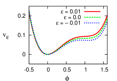
Figure 1: (color online). Potential $v_{\epsilon}(\phi)$ for a few values of $\epsilon$.

We denote a trajectory $\phi(t)$, $0\leq t\leq\infty$, by $[\phi]$. All the statistical quantities of trajectories are described by the path probability measure

$$P([\phi])=\frac{1}{Z_{\phi}}{\rm e}^{-\frac{{\cal F}([\phi])}{T}},$$ (5)

where $Z_{\phi}$ is the normalization factor which is independent of $[\phi]$, and ${\cal F}([\phi])$ is determined as

$${\cal F}([\phi])=\frac{1}{4}\int dt\left(\left((\partial_{t}\phi-f_{\epsilon}(\phi)\right)^{2}+2Tf_{\epsilon}^{\prime}(\phi)\right).$$ (6)

(See Appendix A for its derivation.) The last term in (6) corresponds to the Jacobian associated with the transformation from a noise sequence $[\xi]$ to the corresponding trajectory $[\phi]$.

II.1 Numerical simulations

Before entering the theoretical analysis of (1), we report results of numerical simulations. The Langevin equation was solved numerically with the Heun method heun with a time step $10^{-4}$, and the initial condition was fixed as $\phi(0)=\phi_{0}=1.2$. The expectation value $\left\langle A\right\rangle$ of a fluctuating quantity $A$ was estimated as the average of one-hundred data. By using ten independent samples of the estimated values, the value of $\left\langle A\right\rangle$ is conjectured with error-bars.

In Fig. 2, we display nine trajectories $\phi(t)$ for the system with $\epsilon=0$ and $T=10^{-6}$, where each trajectory is generated by a different noise sequence. The trajectories are clearly distinguished despite a rather small value of $T$. It is seen that a major difference among the trajectories is the exiting time from a region near $\phi=1$. Similar behaviors are observed for other small values of $\epsilon$ and $T$.

In order to clarify $(\epsilon,T)$ dependence of the relaxation behavior, we investigate $\left\langle\phi(t)\right\rangle$ for several values of $\epsilon$ and $T$. As is seen from Fig. 3, $\left\langle\phi(t)\right\rangle$ exhibits the two steps relaxation, and the plateau regime around $\phi\simeq 1$ becomes longer as $T$ is decreased with $\epsilon=0$ fixed (see Fig. 3), or as $\epsilon$ is decreased with $T=2^{-20}$ fixed (see the inset of Fig. 3). These qualitative behaviors are easily conjectured from the form of the potential $v_{\rm\epsilon}(\phi)$.

An impressive feature of the relaxation behavior is qualified by the fluctuation intensity of $\phi(t)$:

$$\chi_{\phi}(t)\equiv T^{-1}(\left\langle\phi^{2}(t)\right\rangle-\left\langle\phi(t)\right\rangle^{2}).$$ (7)

Note that $\chi_{\phi}(t)$ is independent of $T$ in the limit $T\to 0$ when fluctuations are not singular. As displayed in Fig. 4, each $\chi_{\phi}(t)$ for small $\epsilon$ and $T$ takes a maximum value at a time $t_{*}$. Furthermore, it is seen from these graphs that both the time $t_{*}$ and the amplitude $\chi_{\phi}(t_{*})$ increase as $T$ is decreased with $\epsilon=0$ fixed (see Fig. 4) or as $\epsilon$ is decreased with $T=2^{-20}$ fixed (see the inset of Fig. 4).

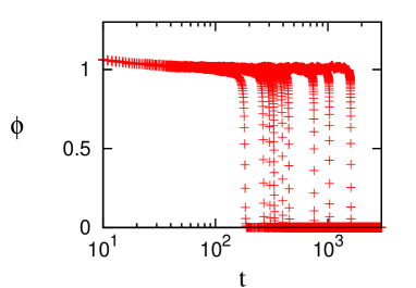
Figure 2: (color online). Trajectories $\phi(t)$ with $\epsilon=0$ and $T=2^{-20}$. The nine trajectories are generated by different noise sequences, respectively.

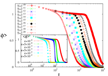
Figure 3: (color online). $\left\langle\phi(t)\right\rangle$ for several values of $T$. $\epsilon=0$. Inset: $\left\langle\phi(t)\right\rangle$ for several values of $\epsilon$. $T=2^{-20}$.

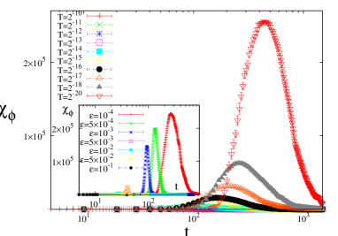
Figure 4: (color online). $\chi_{\phi}(t)$ for several values of $T$. $\epsilon=0$. Inset: $\chi_{\phi}(t)$ for several values of $\epsilon$. $T=2^{-20}$.

Now, we describe the divergent behaviors of $t_{*}$ and $\chi_{\phi}(t_{*})$ quantitatively. We first note that the behaviors are classified into two regimes, (i) $\epsilon\ll T^{2/3}\ll 1$ and (ii) $T^{2/3}\ll\epsilon\ll 1$. We observe

$$t_{*} \simeq T^{-1/3},$$ (8)

$$\chi_{\phi}(t_{*}) \simeq T^{-1},$$ (9)

in the regime (i), while

$$t_{*} \simeq \epsilon^{-1/2},$$ (10)

$$\chi_{\phi}(t_{*}) \simeq \epsilon^{-5/2},$$ (11)

in the regime (ii). The relations (8) and (9) are conjectured from the graphs in the mainframes of Figs. 5 and 6, respectively. Indeed, all the data of $t_{*}T^{1/3}$ and $\chi_{\rm\phi}(t_{*})T$ seem to coincide with each other in the regime $\epsilon T^{-2/3}\ll 1$ for different small values of $T$. The graphs in the insets of Figs. 5 and 6 also indicate the relations (10) and (11) in the limit $T\to 0$ with small $\epsilon$ fixed.

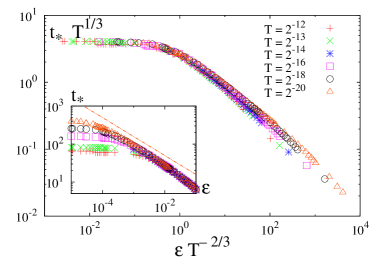
Figure 5: (color online). $t_{*}T^{1/3}$ as functions of $\epsilon T^{-2/3}$ for several values of $T$. Inset: $t_{*}$ as functions of $\epsilon$. The guide line represents a power-law function $t_{*}\simeq\epsilon^{-1/2}$.

Figure 6: (color online). $\chi_{\phi}(t_{*})T$ as functions of $\epsilon T^{-2/3}$ for several values of $T$. Inset: $\chi_{\phi}(t_{*})$ as functions of $\epsilon$. The guide line represents a power-law function $\chi_{\rm\phi}(t_{*})\simeq\epsilon^{-5/2}$.

The specific purpose of this paper is to provide a theoretical understanding of the divergent behaviors given by (8), (9), (10), and (11). Here, we note that $\left\langle\phi(t)\right\rangle$ exhibits the discontinuous behavior from $\epsilon=0$ to $\epsilon\to 0+$ with $T=0$ fixed or from $T=0$ to $T\to 0+$ with $\epsilon=0$ fixed. The coexistence of the discontinuous nature of $\left\langle\phi(t)\right\rangle$ and the critical nature of $\chi_{\phi}(t_{*})$ is a characteristic feature of stochastic dynamics near a saddle-node bifurcation. Such a coexistence, which is called a mixed order transition, has been observed in several systems in the context of dynamical heterogeneity chi4_allstar1 ; chi4_allstar2 ; silbert_mix ; Toninelli_b ; toninelli ; schwartz ; sellitto . See a related discussion in Sec. V.

III phenomenological analysis

In this section, we present a phenomenological argument for deriving the relations (8), (9), (10), and (11). This argument also provides an essential idea behind a systematic perturbation method which will be presented in Sec. IV.

We first note that there are two small parameters $\epsilon$ and $T$ in this problem. Despite of this fact, the discontinuous nature of $\left\langle\phi(t)\right\rangle$ causes difficulties in the theoretical analysis. Indeed, we need a special idea so as to develop a perturbation method. Let us recall the typical trajectories displayed in Fig. 2. All the trajectories are kinked in the time direction. Here, the kink position, which corresponds to the exiting time from a region around $\phi=1$, fluctuates more largely than the other parts of the trajectories. These observations lead to a natural idea that a kink-like trajectory is first identified as an unperturbed state.

We illustrate the idea more concretely. Let us consider two special solutions of $\partial_{t}\phi=f_{0}(\phi)$. The first is the special solution $\phi_{\rm sp}(t)$ under the conditions $\phi_{\rm sp}(t)\to 1$ as $t\to-\infty$, $\phi_{\rm sp}(t)\to 0$ as $t\to\infty$, and $\phi_{\rm sp}(0)=1/2$. $\phi_{\rm sp}(t)$ takes a kink-like form that connects the two fixed points. (See Fig. 7.) The second one is the special solution $\phi_{{\rm B}0}(t)$ under the conditions $\phi_{{\rm B}0}(0)=\phi_{0}$ and $\phi_{{\rm B}0}(t)\to 1$ as $t\to\infty$. $\phi_{{\rm B}0}(t)$ connects the initial value and the marginal saddle. (See Fig. 7.) Then, by introducing a time $\theta$ which corresponds to a kink position, we express trajectories as

$$\phi(t)=\phi_{\rm sp}(t-\theta)+(\phi_{{\rm B}0}(t)-1)+\varphi(t-\theta),$$ (12)

where $\varphi(t-\theta)$ represents deviation from the superposition of the two special solutions.

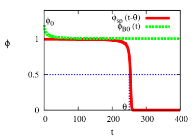
Figure 7: (color online). Functional forms of $\phi_{\rm sp}(t-\theta)$ and $\phi_{\rm B0}(t)$.

Now, fluctuations of $\phi(t)$ are expressed in terms of those of $\theta$ and $\varphi$. Then, it is reasonable to assume that $\varphi$ does not contribute largely to the divergent part of the fluctuation intensity of $\phi(t)$. With this assumption, $\left\langle\phi(t)\right\rangle$ and $\chi_{\phi}(t)$ are estimated as

$$\left\langle\phi(t)\right\rangle=\left\langle\phi_{\rm sp}(t-\theta)\right\rangle,$$ (13)

and

$$\chi_{\phi}(t)=\frac{1}{T}\left(\left\langle\phi_{\rm sp}(t-\theta)^{2}\right\rangle-\left\langle\phi_{\rm sp}(t-\theta)\right\rangle^{2}\right),$$ (14)

where the statistical average is taken over $\theta$ with a distribution function of $\theta$. On the basis of these expressions, we provide a phenomenological argument by which we can determine the exponents characterizing the divergent behavior of $t_{*}$ and $\chi_{\phi}(t_{*})$.

The argument is divided into three parts. In Sec. III.1, we first derive the scaling forms of $\left\langle\theta\right\rangle$ and $\left\langle(\theta-\left\langle\theta\right\rangle)^{2}\right\rangle$ in the two regimes, $T^{2/3}\ll\epsilon\ll 1$ and $\epsilon\ll T^{2/3}\ll 1$, respectively. Second, based on these expressions, we conjecture the distribution functions $P(\theta)$ for the two regimes. Finally, in Sec. III.2, by using $P(\theta)$, we calculate the critical exponents of $t_{*}$ and $\chi_{\phi}(t_{*})$, which were observed numerically in (8), (9), (10), and (11).

III.1 Statistical properties of $\theta$

The fluctuation intensity of $\theta$ is defined as

$$\chi_{\theta}\equiv\frac{1}{T}(\left\langle\theta^{2}\right\rangle-\left\langle\theta\right\rangle^{2}).$$ (15)

We then assume scaling relations

$$\left\langle\theta\right\rangle = T^{-\zeta^{\prime}/\nu_{*}}f_{1}(T^{-1/\nu_{*}}\epsilon),$$ (16)

$$\chi_{\theta} = T^{-\gamma^{\prime}/\nu_{*}}f_{2}(T^{-1/\nu_{*}}\epsilon),$$ (17)

for small $\epsilon$ and $T$, with new exponents $\zeta^{\prime}$, $\nu_{*}$, and $\gamma^{\prime}$. Here, the scaling functions $f_{1}(x)$ and $f_{2}(x)$ satisfy two conditions: (i) $f_{1}(0)$ and $f_{2}(0)$ are finite and (ii) $f_{1}(x)\simeq x^{-\zeta^{\prime}}$ and $f_{2}(x)\simeq x^{-\gamma^{\prime}}$ for $x\gg 1$. The latter condition implies that $\left\langle\theta\right\rangle$ and $\chi_{\theta}$ are independent of T in the regime $T^{1/\nu_{*}}\ll\epsilon\ll 1$, where $\theta$ is expected to obey a Gaussian distribution with variance proportional to $T$ (see (27)).

We shall determine the exponents $\zeta^{\prime}$, $\nu_{*}$, and $\gamma^{\prime}$ in (16) and (17). Since a characteristic time around the marginal saddle is expected to obey the same scaling relation as $\theta$, we investigate the local behavior near $\phi=1$. Concretely, we substitute $\phi=1+\varphi$ into (6) and ignore higher powers of $\varphi$ from an assumption that $|\varphi|$ is small. We then obtain the probability measure for $[\varphi]$ as

$$P\left([\varphi]\right)=\exp\left(-{\tilde{\cal F}}([\varphi])/T\right),$$ (18)

where

$$\tilde{\cal F}([\varphi])=\frac{1}{4}\int dt\left(\left((\partial_{t}\varphi+\epsilon+\varphi^{2}\right)^{2}-4T\varphi\right)+{\rm const}.$$ (19)

From this expression, when $T=0$, we immediately find that $\varphi$ has a scaling form $\varphi(t)=\epsilon^{1/2}\bar{\varphi}_{1}(\epsilon^{1/2}t)$. Since the characteristic time scale in this case diverges as $\epsilon^{-1/2}$, we find that $\zeta^{\prime}=1/2$. On the other hand, when $\epsilon=0$, we obtain another scaling form $\varphi(t)=T^{1/3}\bar{\varphi}_{2}(T^{1/3}t)$ which leads to $\zeta^{\prime}/\nu_{*}=1/3$. We thus derive $\nu_{*}=3/2$. From this result, we expect that a distribution function of $\theta$ is expressed as a $T$-independent function of $\theta T^{1/3}$ when $\epsilon=0$. This expectation leads to a relation $\gamma^{\prime}/\nu_{*}=2\zeta^{\prime}/\nu_{*}+1$, which yields $\gamma^{\prime}=5/2$. These results are summarized as

$$\left\langle\theta\right\rangle = T^{-1/3}f_{1}(\epsilon T^{-2/3}),$$ (20)

$$\chi_{\theta} = T^{-5/3}f_{2}(\epsilon T^{-2/3}),$$ (21)

which, in particular, involve the results

$$\left\langle\theta\right\rangle \simeq T^{-1/3},$$ (22)

$$\chi_{\theta} \simeq T^{-5/3},$$ (23)

in the regime $\epsilon\ll T^{2/3}\ll 1$, while

$$\left\langle\theta\right\rangle \simeq \epsilon^{-1/2},$$ (24)

$$\chi_{\theta} \simeq \epsilon^{-5/2},$$ (25)

in the regime $T^{2/3}\ll\epsilon\ll 1$. As shown in Figs. 8 and 9, numerical results are consistent with (20) and (21).

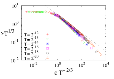
Figure 8: (color online). $\left\langle\theta\right\rangle T^{1/3}$ as functions of $\epsilon T^{-2/3}$. The guide line represents $\left\langle\theta\right\rangle=2\left(6^{1/4}\right)\epsilon^{-1/2}$, which is our theoretical result (131). The graphs for six different values of $T$ tend to converge to one curve as $T$ is decreased.

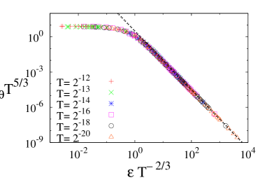
Figure 9: (color online). $\chi_{\rm\theta}T^{5/3}$ as functions of $\epsilon T^{-2/3}$. The guide line represents $\chi_{\rm\theta}=2\left(6^{1/4}\right)\epsilon^{-5/2}$, which is our theoretical result (132). The graphs for six different values of $T$ are on one curve.

Based on these results (22), (23), (24), and (25), we conjecture functional forms of $P(\theta)$ from which we will calculate $\chi_{\phi}(t)$.

First, we consider the regime $\epsilon\ll T^{2/3}\ll 1$. In order to simplify the argument, we focus on the case that $\epsilon=0$ and $T\ll 1$, as the representative in the regime $\epsilon\ll T^{2/3}\ll 1$. In this case, an exiting event from a region near $\phi=1$ occurs by effects of small noise. We then naturally expect that trajectories reach to $\phi=1/2$ randomly as a Poisson process except for a short time regime in which the behavior depends on initial conditions. That is, we conjecture that $\theta$ obeys the Poisson distribution when $\theta$ is much larger than some cut-off value $\theta_{\rm cut}$. Furthermore, from (22) and (23), the distribution function $P(\theta)$ is expressed as $P(\theta)={\tilde{P}}(\theta T^{1/3})$. These considerations lead to

$$P(\theta)=\frac{T^{1/3}{\rm e}^{-a\theta T^{1/3}}}{Z_{\theta}^{(1)}}$$ (26)

for the regime $\theta>\theta_{\rm cut}$. The positive constant $a$ and the normalization constant $Z_{\theta}^{(1)}$ are independent of $T$. We also assume that $\theta_{\rm cut}=O(T^{-1/3})$, which means $\int^{\infty}_{\theta_{\rm cut}}d\theta P(\theta)\not=1$ in the limit $T\to 0$. We thus introduce a $T$-independent parameter as $\tilde{\theta}_{\rm cut}=\theta_{\rm cut}T^{1/3}$. The expression (26) will be derived in Sec. IV.

Next, we consider the regime $T^{2/3}\ll\epsilon\ll 1$. When $\epsilon\neq 0$ and $T=0$, $P(\theta)$ is the delta function $\delta(\theta-\left\langle\theta\right\rangle)$, because there are no fluctuations. For sufficiently small $T$, the distribution function is smeared slightly, and this leads to a conjecture that $\theta$ obeys a Gaussian distribution

$$P(\theta)=\frac{1}{Z_{\theta}^{(2)}}{\rm e}^{-\frac{1}{T}\frac{\left(\theta-\left\langle\theta\right\rangle\right)^{2}}{2\chi_{\theta}}},$$ (27)

where $Z_{\theta}^{(2)}$ is a normalization constant. The expression (27) will be derived in Sec. IV.

III.2 Calculation of $\chi_{\phi}(t)$

On the basis of the results (26) and (27), we calculate the critical exponents of $t_{*}$ and $\chi_{\phi}(t_{*})$. Here, for convenience of calculation, we introduce the Fourier transform of $\phi_{\rm sp}(t)$ as

$$\phi_{\rm sp}(t)=\int\frac{d\omega}{2\pi}\tilde{\phi}_{\rm sp}(\omega){\rm e}^{i\omega t}.$$ (28)

Then, from the assumptions (13) and (14), we estimate

$$\left\langle\phi(t)\right\rangle = \int\frac{d\omega}{2\pi}\tilde{\phi}_{\rm sp}(\omega){\rm e}^{i\omega t}\left\langle{\rm e}^{-i\omega\theta}\right\rangle,$$ (29)

and

$$\left\langle\phi(t)^{2}\right\rangle = \int\frac{d\omega}{2\pi}\int\frac{d\omega^{\prime}}{2\pi}\tilde{\phi}_{\rm sp}(\omega)\tilde{\phi}_{\rm sp}(\omega^{\prime}){\rm e}^{i(\omega+\omega^{\prime})t}$$ (30)

$$\left\langle{\rm e}^{-i(\omega+\omega^{\prime})\theta}\right\rangle.$$

By substituting (29) and (30) into (7), we obtain

$$\chi_{\phi}(t) = \frac{1}{T}\int\frac{d\omega}{2\pi}\int\frac{d\omega^{\prime}}{2\pi}\tilde{\phi}_{\rm sp}(\omega)\tilde{\phi}_{\rm sp}(\omega^{\prime}){\rm e}^{i(\omega+\omega^{\prime})t}$$ (31)

$$\left(\left\langle{\rm e}^{-i(\omega+\omega^{\prime})\theta}\right\rangle-\left\langle{\rm e}^{-i\omega\theta}\right\rangle\left\langle{\rm e}^{-i\omega^{\prime}\theta}\right\rangle\right).$$

In the following paragraphs, we shall calculate $\chi_{\phi}(t)$ for the two regimes $T^{2/3}\ll\epsilon\ll 1$ and $\epsilon\ll T^{2/3}\ll 1$, respectively.

First, we consider the regime $\epsilon\ll T^{2/3}\ll 1$ with setting $\epsilon=0$. By using the distribution function (26), we have

$$\left\langle{\rm e}^{-i\omega\theta}\right\rangle = \int_{0}^{\theta_{\rm cut}}d\theta e^{-i\omega\theta}P(\theta)$$ (32)

$$+ \int_{\theta_{\rm cut}}^{\infty}d\theta\frac{T^{1/3}{\rm e}^{-a\theta T^{1/3}-i\omega\theta}}{Z_{\theta}^{(1)}}.$$

We assume that the first term of (32) is neglected when $T\ll 1$. Then, by performing the integration, we calculate

$$\left\langle{\rm e}^{-i\omega\theta}\right\rangle = \frac{T^{1/3}}{Z_{\theta}^{(1)}}\left[\frac{e^{-\theta_{\rm cut}T^{1/3}(a+i\omega T^{-1/3})}}{T^{1/3}\left(a+iT^{-1/3}\omega\right)}\right].$$ (33)

Similarly, we obtain

$$\left\langle{\rm e}^{-i(\omega+\omega^{\prime})\theta}\right\rangle = \frac{T^{1/3}}{Z_{\theta}^{(1)}}\left[\frac{e^{-\theta_{\rm cut}T^{1/3}(a+i\left(\omega+\omega^{\prime}\right)T^{-1/3})}}{T^{1/3}\left(a+iT^{-1/3}\left(\omega+\omega^{\prime}\right)\right)}\right].$$

Furthermore, since $\phi_{\rm sp}(t)$ shows a quick change from $\phi_{\rm sp}(t)=1$ to $\phi_{\rm sp}(t)=0$ around the kink position $t=\theta$, we approximate $\phi_{\rm sp}(t)$ as $\Theta(-t)$, where $\Theta(t)$ is the Heaviside step function. With this approximation, the Fourier transform of $\phi_{\rm sp}(t)$ becomes

$${\tilde{\phi}_{\rm sp}}(\omega)=\lim_{b\to 0+}\frac{-1}{i\omega-b}.$$ (35)

Here, we introduce a scaled time ${\tilde{t}}=tT^{1/3}$. We then substitute (33), (LABEL:theta_poisson2), and (35) into (31). The result is

$$\chi_{\phi}(\tilde{t}T^{-1/3})$$ (36)

$$= \frac{1}{T}\int\frac{d\omega}{2\pi}\int\frac{d\omega^{\prime}}{2\pi}\lim_{b\to 0+}\frac{1}{i\omega-b}\frac{1}{i\omega^{\prime}-b}{\rm e}^{i(\omega+\omega^{\prime})T^{-1/3}(\tilde{t}-\tilde{\theta}_{\rm cut})}$$

$$\left(\frac{1}{Z_{\theta}^{(1)}}\left[\frac{e^{-\tilde{\theta}_{\rm cut}a}}{\left(a+iT^{-1/3}\left(\omega+\omega^{\prime}\right)\right)}\right]\right.$$

$$-\left.\frac{1}{\left(Z_{\theta}^{(1)}\right)^{2}}\left[\frac{e^{-2\tilde{\theta}_{\rm cut}a}}{\left(a+iT^{-1/3}\omega\right)\left(a+iT^{-1/3}\omega^{\prime}\right)}\right]\right).$$

By the transformation of integrable variables, ${\tilde{\omega}}=\omega T^{-1/3}$ and ${\tilde{\omega}^{\prime}}=\omega^{\prime}T^{-1/3}$, $\chi_{\phi}(t)$ is expressed as a scaling form $\chi_{\phi}(t)=\tilde{\chi}_{\phi}(T^{1/3}t-\tilde{\theta}_{\rm cut})/T$. This implies that $t_{*}=O(T^{-1/3})$ and $\chi_{\phi}(t_{*})=O(T^{-1})$ in the limit $T\to 0$. Furthermore, we expect that these exponents are valid for $\epsilon$ and $T$ that satisfy $\epsilon\ll T^{2/3}\ll 1$. In this manner, we have obtained the results consistent with (8) and (9).

We next consider the regime $T^{2/3}\ll\epsilon\ll 1$ by using the distribution function (27). The Gaussian integration with respect to $\theta$ leads to

$$\left\langle{\rm e}^{-i\omega\theta}\right\rangle = {\rm e}^{-i\omega\left\langle\theta\right\rangle}{\rm e}^{-\frac{\chi_{\theta}\omega^{2}T}{2}},$$ (37)

and

$$\left\langle{\rm e}^{-i(\omega+\omega^{\prime})\theta}\right\rangle = {\rm e}^{-i(\omega+\omega^{\prime})\left\langle\theta\right\rangle}{\rm e}^{-\frac{\chi_{\theta}(\omega+\omega^{\prime})^{2}T}{2}}.$$ (38)

Then, by substituting (37) and (38) into (29) and (31), we obtain

$$\left\langle\phi(t)\right\rangle=\int\frac{d\omega}{2\pi}\tilde{\phi}_{\rm sp}(\omega){\rm e}^{i\omega(t-\left\langle\theta\right\rangle)}{\rm e}^{-\frac{\chi_{\theta}\omega^{2}T}{2}},$$ (39)

and

$$\chi_{\phi}(t) = \frac{1}{T}\int\frac{d\omega}{2\pi}\int\frac{d\omega^{\prime}}{2\pi}\tilde{\phi}_{\rm sp}(\omega)\tilde{\phi}_{\rm sp}(\omega^{\prime}){\rm e}^{i(\omega+\omega^{\prime})(t-\left\langle\theta\right\rangle)}$$ (40)

$$\left({\rm e}^{-\frac{\chi_{\theta}(\omega+\omega^{\prime})^{2}T}{2}}-{\rm e}^{-\frac{\chi_{\theta}(\omega^{2}+\omega^{\prime 2})T}{2}}\right).$$

From these, we derive

$$\chi_{\phi}(t) = \chi_{\theta}\sum_{k=1}^{\infty}\frac{1}{k!}\left(\left(\sqrt{\chi_{\theta}T}\right)^{k-1}\partial_{t}^{k}\left\langle\phi(t)\right\rangle\right)^{2}.$$ (41)

Here, let $\tau_{\rm w}=\sqrt{\chi_{\theta}T}$ be the width of the distribution of $\theta$. When $\tau_{\rm w}\ll 1$, the expressions (39) and (41) are further simplified. Indeed, we may estimate

$$\left\langle\phi(t)\right\rangle=\phi_{\rm sp}(t-\left\langle\theta\right\rangle),$$ (42)

and

$$\chi_{\phi}(t)=\chi_{\theta}(\partial_{t}\phi_{\rm sp}(t-\left\langle\theta\right\rangle))^{2}.$$ (43)

These results show that $\chi_{\phi}(t)$ takes a maximum at $t=t_{*}$, where $t_{*}\simeq\left\langle\theta\right\rangle\simeq\epsilon^{-1/2}$. Furthermore, we obtain $\chi_{\phi}(t_{*})\simeq\chi_{\theta}\simeq\epsilon^{-5/2}$. These results are consistent with (10) and (11). Note that they are valid in the regime $\tau_{\rm w}\ll 1$ which means $T^{2/5}\ll\epsilon\ll 1$. It seems that there is no power-law behavior in the regime $T^{2/3}\ll\epsilon\ll T^{2/5}$. In fact, Fig. 6 suggests that $\chi_{\phi}(t_{*})$ does not converge to one universal curve in the whole region.

To this point, we have explained that the singular behavior of $\chi_{\phi}(t)$ is determined by the statistical distribution of $\theta$. Our analysis shows that $\theta$ is the most important quantity for characterization of the divergent fluctuations near the saddle-node bifurcation. This claim is also conjectured from a fact that the statistical properties of $\theta$ are simpler than those of $\phi$. (Compare Figs. 5 and 6 with Figs. 8 and 9.) Thus, we have focused our theoretical analysis on the derivation of the statistical properties of $\theta$. Note that the scaling relations (22) and (24) were derived in Refs. kubokitahara ; binder , and arguments closely related to (23) and (25) were also presented in Refs. reimann ; spike . In particular, all the statistical properties of $\theta$ are described by the analysis of the backward Fokker-Planck equation Gardner . However, in the previous approaches, a perturbative calculation with small $\epsilon$ and $T$ seems quite complicated. In such cases, it would be almost impossible to analyze spatially extended systems. In order to improve the situation, in the next section, we develop a systematic perturbative calculation for the distribution function of $\theta$ within the path-integral formulation (5) with (6).

IV Analysis

Our theory basically relies on the idea mentioned in Sec. III. That is, we start with the expression (12) and derive the distribution function of the exiting time $\theta$. Formally, the derivation might be done by performing the integration of $P([\phi])$ with respect to $\varphi$ with $\theta$ fixed. However, as far as we attempt, it seems difficult to carry out this integration by a standard path integral method. One difficulty originates from the existence of a transient region before passing the marginal saddle. This contribution is described by the interaction of $\phi_{{\rm B}0}$ and $\theta$, and yields a non-trivial distribution of $\theta$ in the regime $\theta\ll\left\langle\theta\right\rangle$. The other difficulty arises in calculation of a perturbative expansion around the solution $\phi_{\rm sp}$. Since the solution approaches the marginal saddle in the limit $t\to-\infty$, the stability of the solution is marginal. In such a case, a naive perturbation induces a singularity. We thus need to reformulate the perturbation problem.

In order to overcome the two difficulties, in this paper, we employ a method of fictitious stochastic processes fictitious . Concretely, we introduce a variable $\phi(t,s)$ with a fictitious time $s$ and define a fictitious Langevin equation whose $s$-stationary distribution function is equal to the path probability measure given in (5). The Langevin equation is written as

$$\partial_{s}\phi(t,s)=-\frac{\delta{\cal F}([\phi])}{\delta\phi}+\sqrt{2T}\eta(t,s),$$ (44)

with

$$\left\langle\eta(t,s)\eta(t^{\prime},s^{\prime})\right\rangle=\delta(t-t^{\prime})\delta(s-s^{\prime}).$$ (45)

By substituting (6) into (44), we write explicitly

$$\partial_{s}{\phi} = \frac{1}{2}\partial_{t}^{2}\phi-F_{\epsilon,T}(\phi)+\sqrt{2T}\eta(t,s),$$ (46)

where

$$F_{\epsilon,T}(\phi) = \frac{f^{\prime}_{\epsilon}(\phi)f_{\epsilon}(\phi)}{2}+\frac{T}{2}f_{\epsilon}^{\prime\prime}(\phi)$$ (47)

$$= \frac{1}{2}\phi(3\phi-1)(\phi-1)^{3}+J_{T}(\phi)+G_{\epsilon}(\phi),$$

with

$$J_{T}(\phi) = -\frac{T}{2}(6\phi-4),$$

$$G_{\epsilon}(\phi) = \frac{1}{2}\epsilon^{2}\phi+\epsilon\phi(\phi-1)(2\phi-1).$$ (48)

By interpreting $t$ as a fictitious space coordinate, we regard (46) as a reaction-diffusion system with the boundary condition $\phi(0,s)=\phi_{0}$. Particularly, since the system is bistable, one may employ techniques treating kinks in such systems ohtakawasaki ; eiohta . As a result, as will be shown in subsequent sections, the interaction between $\phi_{{\rm B}0}$ and $\theta$ can be formulated as a perturbation and the problem arising from the marginal stability of $\phi_{\rm sp}$ can be treated in a proper manner. We note that interesting noise effects in kink dynamics in bistable systems were reported in Ref. polymer .

As discussed in Sec. II, the qualitatively different behaviors were observed depending on the regime either $\epsilon\ll T^{2/3}\ll 1$ or $T^{2/3}\ll\epsilon\ll 1$. Correspondingly, the perturbation theory is developed for each regime. Since the basic idea behind calculation details is in common to both the regimes, we provide the full account of the perturbation theory for the regime $\epsilon\ll T^{2/3}\ll 1$ in Sec. IV.1, IV.2, and IV.3. Then, we discuss briefly a perturbation theory for the regime $T^{2/3}\ll\epsilon\ll 1$ with pointing out the difference from the regime $\epsilon\ll T^{2/3}\ll 1$ in Sec. IV.4.

IV.1 Formulation

IV.1.1 Unperturbed system

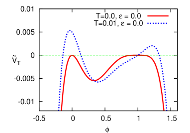
Figure 10: (color online). Potential $\tilde{V}_{T}(\phi)$ for $T=0$ and $T=0.01$.

Since we focus on the regime $\epsilon\ll T^{2/3}\ll 1$, one may choose the system with $\epsilon=0$ and $T=0$ as an unperturbed system. However, we cannot develop a perturbation theory with this choice. In order to explain the reason more explicitly, we define a potential function $\tilde{V}_{T}(\phi)$ by

$$F_{\epsilon=0,T}(\phi)=-\partial_{\phi}\tilde{V}_{T}(\phi),$$ (49)

where $\tilde{V}_{T}(1)=0$. This potential is calculated as

$$\tilde{V}_{T}(\phi)=-\frac{1}{4}\phi^{2}(\phi-1)^{4}+\frac{T}{2}(\phi-1)(3\phi-1).$$ (50)

In Fig. 10, the functional forms of $\tilde{V}_{T}(\phi)$ are displayed for $T=0$ and $T=0.01$. Here, the special solution $\phi_{\rm sp}(t)$ in (12) connects the two maxima of $\tilde{V}_{T=0}(\phi)$. However, since the curvature of the potential $\tilde{V}_{T=0}(\phi)$ at the maximal point $\phi=1$ is zero, a perturbative correction to the solution $\phi_{\rm sp}(t)$ exhibits a divergent behavior. (See an argument below (88).) In order to avoid the singularity, we must choose an unperturbed potential different from $\tilde{V}_{T=0}(\phi)$. Based on a fact that $\tilde{V}_{T}(\phi)$ has the two maxima at $\phi=\phi_{1}=-4T+O(T^{2})$ and $\phi=\phi_{2}=1+T^{1/3}+O(T^{2/3})$, where $\tilde{V}_{T}(\phi_{1})=T/2$ and $\tilde{V}_{T}(\phi_{2})=3T^{4/3}/4+O(T^{5/3})$, we define an unperturbed potential $V_{\rm u}$ by the decomposition

$$\tilde{V}_{T}(\phi)=V_{\rm u}(\phi)+\Delta(\phi),$$ (51)

where $\Delta(\phi)$ is chosen such that the two maximal values at $\phi=\phi_{1}$ and $\phi=\phi_{2}$ of $V_{u}(\phi)$ are identical; that is, $V_{\rm u}(\phi_{1})=V_{\rm u}(\phi_{2})=T/2$ and $V_{\rm u}^{\prime}(\phi_{1})=V_{\rm u}^{\prime}(\phi_{2})=0$, as shown in Fig. 11. Furthermore, in order to have a simple argument, we impose a condition that the curvature at each maximum of $V_{\rm u}$ is equal to that of the corresponding maximum of $\tilde{V}_{T}$ with ignoring contribution of $O(T^{4/3})$. These conditions are satisfied by setting $\Delta(\phi_{1})=0$, $\Delta(\phi_{2})=\tilde{V}_{T}(\phi_{2})-\tilde{V}_{T}(\phi_{1})=3T^{4/3}/4-T/2+O(T^{5/3})$, $\Delta^{\prime}(\phi_{1})=\Delta^{\prime}(\phi_{2})=0$, $\Delta^{\prime\prime}(\phi_{1})=O(T^{4/3})$, and $\Delta^{\prime\prime}(\phi_{2})=O(T^{5/3})$. As an example, one may choose

$$\Delta(\phi)=\left(\frac{3}{4}T^{4/3}-\frac{T}{2}+O(T^{5/3})\right)(12v_{\epsilon=0}(\phi)+O(T)).$$ (52)

By using the decomposition (51) and defining $F_{\rm u}\equiv-\partial_{\phi}V_{\rm u}$, we rewrite (46) as

$$\partial_{s}\phi = \frac{1}{2}\partial_{t}^{2}{\phi}-F_{\rm u}(\phi)-G_{\epsilon}(\phi)+\Delta^{\prime}(\phi)+\sqrt{2T}\eta.$$ (53)

In our formulation, we treat the last three terms as perturbations.

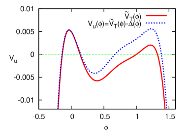
Figure 11: (color online). Unperturbative potential $V_{\rm u}(\phi)$, and ${\tilde{V}}_{T}(\phi)$ for $T=0.01$.

IV.1.2 Expression of solutions

Since we have replaced the unperturbative potential, we reconsider an expression of trajectories. We first define the special solution $\phi_{*}$ of the unperturbed equation

$$\frac{1}{2}\frac{d^{2}\phi_{*}}{dt^{2}}-F_{\rm u}(\phi_{*})=0$$ (54)

under the conditions $\phi_{*}(t)\to\phi_{2}$ when $t\to-\infty$ and $\phi_{*}(t)\to\phi_{1}$ when $t\to\infty$. We also impose $\phi_{*}(0)=1/2$ in order to determine $\phi_{*}$ uniquely. This solution corresponds to the kink solution in the real time direction and describes the relaxation behavior from $\phi=\phi_{2}(\simeq 1)$ to $\phi=\phi_{1}(\simeq 0)$. The functional form of $\phi_{*}$ can be obtained by the integration of

$$\partial_{t}\phi_{*}=-2\sqrt{V_{\rm u}(\phi_{1})-V_{\rm u}(\phi_{*})}.$$ (55)

In Fig. 12, we show $\phi_{*}(t)$ for $T=10^{-3}$ and $10^{-5}$.

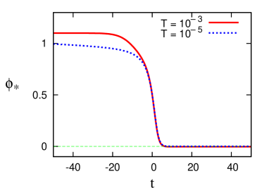
Figure 12: (color online). $\phi_{*}$ as functions of $t$.

Next, let $\phi_{\rm B}$ be the solution of

$$\frac{1}{2}\frac{\partial^{2}\phi_{\rm B}}{\partial t^{2}}-F_{\rm u}(\phi_{\rm B})=0$$ (56)

under the conditions that $\phi_{\rm B}(t)\to\phi_{2}$ as $t\to\infty$ and that $\phi_{\rm B}(0)=\phi_{0}$. This solution describes a typical behavior of $\phi$ near $t=0$ when $T$ is sufficiently small. By using these two solutions, we express the solution of (53) for a given $\eta$ as

$$\phi(t,s)=\phi_{*}(t-\theta(s))+(\phi_{\rm B}(t)-\phi_{2})+\rho(t-\theta(s),s),$$ (57)

where $\rho$ represents a possibly small deviation from the superposition of the two solutions.

IV.1.3 Linear stability analysis

Figure 13: (color online). $F^{\prime}_{\rm u}(\phi_{*}(u))$ as functions of $u$.

As a preliminary for a systematic perturbation theory, we perform the linear stability analysis of $\phi_{*}$. Hereafter, we set $u=t-\theta$. The stability of the solution $\phi_{*}$ is determined by eigenvalues of the linear operator $\hat{L}$ given by

$$\hat{L}\equiv\frac{1}{2}\frac{d^{2}}{du^{2}}-F^{\prime}_{u}(\phi_{*}(u)).$$ (58)

Let us consider the eigenvalue problem

$$\hat{L}\Phi(u)=-\lambda\Phi(u).$$ (59)

This problem is equivalent to an energy eigenvalue problem in one-dimensional quantum mechanics, where $F_{u}^{\prime}(\phi_{*}(u))$ and $\lambda$ correspond to the potential and an energy eigenvalue, respectively. The graphs of $F_{u}^{\prime}(\phi_{*}(u))$ are shown in Fig. 13. The asymptotic behaviors are calculated as $F_{u}^{\prime}(\phi_{*}(u))\to 1/2+O(T)$ as $u\to\infty$, and $F_{u}^{\prime}(\phi_{*}(u))\to 3T^{2/3}+O(T)$ as $u\to-\infty$.

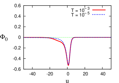
Figure 14: (color online). $\Phi_{0}$ as functions of $u$.

Since $\phi_{*}(t-\theta)$ for any $\theta$ is a solution of (54), we may take the derivative of (54) with respect to $\theta$. We then have

$$\hat{L}\partial_{u}\phi_{*}=0.$$ (60)

This implies that there exists the zero-eigenvalue, for which the normalized eigenfunction $\Phi_{0}(u)$ is determined as

$$\Phi_{0}(u) = \left(\partial_{u}\phi_{*}\right)/\sqrt{\Gamma},$$ (61)

where

$$\Gamma = \int_{-\infty}^{\infty}du(\partial_{u}\phi_{*}(u))^{2}.$$ (62)

Here, by using $\partial_{u}\phi_{*}=f_{\epsilon=0}(\phi_{*})+O(T)$, we obtain

$$\Gamma = \int_{1}^{0}d\phi f_{\epsilon=0}(\phi)+O(T)$$ (63)

$$= v_{\epsilon=0}(\phi)|_{0}^{1}+O(T)$$

$$= \frac{1}{12}+O(T).$$

The zero-eigenfunction $\Phi_{0}(u)$ corresponds to the Goldstone mode associated with a time translational symmetry. The functional form of $\Phi_{0}(u)$ is shown in Fig. 14. Since there is no node in the $u$ profile of $\Phi_{0}(u)$, the minimum eigenvalue must be zero as in quantum mechanics. Since the height of the potential in the limit $u\to-\infty$ is $O(T^{2/3})$, it is expected that there is no other discrete eigenvalue when $T$ is sufficiently small. Next, we consider continuous eigenvalues for $\lambda\geq\lambda_{\rm m}=\lim_{u\to\infty}F_{u}^{\prime}(\phi_{*}(u))=3T^{2/3}+O(T)$. The corresponding eigenfunctions are characterized by the asymptotic plane waves with the eigenvalues $\lambda=\lambda_{\rm m}+k_{\rm L}^{2}/2$ and $\lambda=(1+k_{\rm R}^{2})/2$, where $k_{\rm R}$ and $k_{\rm L}$ are non-zero real numbers representing wavenumbers of the asymptotic plane waves, in the limit $u\to-\infty$ and $u\to+\infty$ respectively.

We denote by $\Phi_{\lambda}(u)$ the eigenfunction corresponding to the eigenvalue $\lambda$. Since the eigenvalues greater than $1/2$ are degenerated, $\Phi_{\lambda}^{*}(u)\not=\Phi_{\lambda}(u)$ for $\lambda\geq 1/2$, where ^∗ represents the complex conjugate. Here, it is convenient to introduce $\Phi_{-\lambda}(u)$ as $\Phi_{-\lambda}(u)=\Phi_{\lambda}^{*}(u)$. Related to this introduction, we also define the index set $\Lambda=\{\lambda|\lambda\leq-1/2,\quad\lambda\geq\lambda_{\rm m}\}$. Then, we may choose the set of eigenfunctions so as to satisfy the orthogonality condition

$$\int_{-\infty}^{\infty}du\Phi_{\lambda^{\prime}}^{*}(u)\Phi_{\lambda}(u)=\delta(\lambda-\lambda^{\prime}),$$ (64)

and

$$\int_{-\infty}^{\infty}du\Phi_{0}(u)\Phi_{\lambda}(u)=0,$$ (65)

for any $\lambda,\lambda^{\prime}\in\Lambda$. Furthermore, we expect the completeness condition

$$\Phi_{0}(u)\Phi_{0}(u^{\prime})+\int_{\Lambda}d\lambda\Phi_{\lambda}^{*}(u)\Phi_{\lambda}(u^{\prime})=\delta(u-u^{\prime}).$$ (66)

By using these eigenfunctions, we expand $\rho(u,s)$ as

$$\rho(u,s)=\int_{\Lambda}d\lambda\psi_{\lambda}(s)\Phi_{\lambda}(u),$$ (67)

where the contribution of the zero eigenfunction is not taken into account in the expression (67) so that the expression (57) is uniquely determined.

IV.2 Perturbation theory

By substituting (57) into (53), we obtain

$$-\Omega\partial_{u}{\phi_{*}}+\partial_{s}\rho$$ (68)

$$= \hat{L}(\phi_{*})\rho-\frac{1}{2}F^{\prime\prime}_{\rm u}(\phi_{*})\rho^{2}$$

$$-G_{\epsilon}(\phi_{*})+\Delta^{\prime}(\phi_{*})$$

$$+\hat{L}(\phi_{*})(\phi_{\rm B}(t)-\phi_{2})+\sqrt{2T}\eta+\cdots,$$

where we set

$$\Omega=\partial_{s}\theta.$$ (69)

We consider a perturbation expansion of $\rho$ and $\Omega$ with respect to a small parameter. In the present problem, $G_{\epsilon}(\phi_{*})$, $\Delta^{\prime}(\phi_{*})$, $\hat{L}(\phi_{*})(\phi_{\rm B}(t)-\phi_{2})$, and $\sqrt{2T}\eta$ are treated as perturbations. In order to formulate the problem concretely, we introduce a formal expansion parameter $\mu$ in front of $G_{\epsilon}(\phi_{*})$, $\Delta^{\prime}(\phi_{*})$, $\hat{L}(\phi_{*})(\phi_{\rm B}(t)-\phi_{2})$, and $T$ in the noise term. We solve the equation (68) perturbatically under the assumption that $\rho$ and $\Omega$ can be expanded in $\mu$. Note that $\rho$=$\Omega$=0 when $\mu=0$. Concretely, due to the small noise term which is $O(\mu^{1/2})$, we assume

$$\Omega = \mu^{1/2}\Omega^{(1/2)}+\mu\Omega^{(1)}+\cdots,$$ (70)

$$\rho = \mu^{1/2}\rho^{(1/2)}+\mu\rho^{(1)}+\cdots.$$ (71)

As we will see below, all the terms of $\rho^{(i)}$ and $\Omega^{(i)}$ can be calculated in principle. Here, it should be noted that $\mu$ is not directly related to small parameters $\epsilon$ and $T$. Therefore, for example, if one wishes to derive the solution valid up to $O(T^{2})$, we do not have a quick answer to the question how many orders of expansion in $\mu$ are necessary. Although this aspect makes the analysis complicated, we will find that the formulation leads to a systematic expansion. These preliminaries presented in this section are standard in a singular perturbation method hohenberg ; kuramoto_p . With this setting up, we calculate $\rho^{(i)}$ and $\Omega^{(i)}$ in sequence.

IV.2.1 Lowest order result

We start with the calculation of $\Omega^{(1/2)}$ and $\rho^{(1/2)}$. We substitute the expansions (70) and (71) into (68), arrange terms according to powers of $\mu$, and pick up all the terms proportional to $O(\mu^{1/2})$. We then obtain

$$-\Omega^{(1/2)}\partial_{u}{\phi_{*}}+\partial_{s}\rho^{(1/2)}=\hat{L}(\phi_{*})\rho^{(1/2)}+\sqrt{2T}\eta.$$ (72)

We rewrite (72) as a linear equation for $\rho^{(1/2)}$ with the expression

$$\left(\partial_{s}-\hat{L}(\phi_{*})\right)\rho^{(1/2)}=B(\phi_{*},\eta).$$ (73)

Because $\hat{L}(\phi_{*})$ possesses the zero-eigenvalue, it is not the case that there exists a unique bounded $\rho^{(1/2)}$. That is, there exists no bounded solution or there are an infinitely number of solutions. In order to proceed the calculation further by obtaining $\rho^{(1/2)}$, we impose the solvability condition under which the latter case is chosen. The solvability condition in this case is written as

$$\int_{-\infty}^{\infty}du\Phi_{0}(u)B(\phi_{*},\eta)=0.$$ (74)

This yields

$$-\Gamma\Omega^{(1/2)}=\sqrt{2T\Gamma}\eta_{\theta},$$ (75)

where

$$\eta_{\theta}(s) = \int_{-\infty}^{\infty}du(\partial_{u}\phi_{*})\eta(u+\theta,s)/\sqrt{\Gamma}.$$ (76)

We note that (76) satisfies

$$\left\langle\eta_{\theta}(s)\eta_{\theta}(s^{\prime})\right\rangle=\delta(s-s^{\prime}).$$ (77)

Furthermore, under the solvability condition, one can determine statistical properties of $\rho^{(1/2)}$ from (73). In a manner similar to (67), we expand $\rho^{(1/2)}$ in terms of the eigenfunctions of $\hat{L}(\phi_{*})$. Then, for any non-zero eigenvalue $\lambda$, the coefficient $\psi_{\lambda}^{(1/2)}$ obeys a Langevin equation

$$\partial_{s}\psi_{\lambda}^{(1/2)}=-\lambda\psi_{\lambda}^{(1/2)}+\sqrt{2T}\eta_{\lambda},$$ (78)

with

$$\eta_{\lambda}(s)=\int_{-\infty}^{\infty}du\Phi_{\lambda}(u)\eta(u+\theta,s).$$ (79)

From this, we obtain $\left\langle\psi_{\lambda}^{(1/2)}\right\rangle_{\rm\theta}=0$ and

$$\left\langle\psi_{\lambda}^{(1/2)}\psi^{(1/2)}_{\lambda^{\prime}}{}^{*}\right\rangle_{\rm\theta}=\frac{T}{\lambda}\delta(\lambda-\lambda^{\prime}),$$ (80)

where $\left\langle\right\rangle_{\rm\theta}$ denotes an expectation value with $\theta$ fixed. The fluctuation intensity of $\rho^{(1/2)}$ is then calculated as

$$\left\langle(\rho^{(1/2)})^{2}\right\rangle_{\theta} = \int_{\Lambda}d\lambda\frac{T}{\lambda}|\Phi_{\lambda}(u)|^{2}$$ (81)

$$= -TG(u,u),$$

where $G(z,y)$ is the Green function defined as

$$G(z,y)=-\int_{\Lambda}d\lambda\frac{1}{\lambda}\Phi_{\lambda}(z)\Phi_{\lambda}^{*}(y).$$ (82)

Here, we note that $G(z,y)$ satisfies

$$\left(\frac{1}{2}\partial_{z}^{2}-F_{\rm u}^{\prime}(\phi_{*}(z))\right)G(z,y)=\delta(z-y)-\Phi_{0}(z)\Phi_{0}(y).$$

Let us estimate $G(u,u)$ in the limit $u\to\pm\infty$ by defining

$$m_{\pm}=\lim_{u\to\pm\infty}\sqrt{2F^{\prime}_{u}(\phi_{*}(u))}.$$ (84)

From the expression of $F_{\rm u}(\phi_{*}(u))$ determined by (47), (51), and (52), we calculate

$$m_{+} = 1+O(T),$$ (85)

$$m_{-} = \sqrt{6}T^{1/3}+O(T^{2/3}),$$ (86)

in the limit $T\to 0$. We then define a Green function $G_{\pm}(z,y)$ by

$$\left(\frac{1}{2}\partial_{z}^{2}-\frac{m_{\pm}^{2}}{2}\right)G_{\pm}(z,y)=\delta(z-y).$$ (87)

This Green function is written as

$$G_{\pm}(z,y)=-\frac{1}{m_{\pm}}{\rm e}^{-m_{\pm}|z-y|}.$$ (88)

We conjecture that $G(u,u)$ approaches $G_{\pm}(u,u)$ as $u\to\pm\infty$. Then, from (81), we find that $\left\langle(\rho^{(1/2)})^{2}\right\rangle_{\theta}\simeq O(T^{2/3})$ for $u\to-\infty$, and $\left\langle(\rho^{(1/2)})^{2}\right\rangle_{\theta}\simeq O(T)$ for $u\to\infty$.

Here, we address one remark. If $\phi_{\rm sp}(t)$ were chosen as the unperturbative solution, $m_{-}$ would become zero, and therefore $\rho^{(1/2)}(u\simeq-\infty)$ would exhibit unbounded Brownian motion as a function of $s$. This singularity originates from the marginal stability of $\phi_{\rm sp}$. This is why we choose $\phi_{*}$ instead of $\phi_{\rm sp}$ as the unperturbative solution, which was mentioned in Sec. IV.1.1.

IV.2.2 Next order calculation

In the lowest order description, the variable $\theta$ exhibits unbounded Brownian motion, and therefore it indicates a singular behavior. Now, in order to determine the exponents characterizing the singularity, we proceed to the next order calculation. We substitute (70) and (71) into (68) and pick up all the terms proportional to $O(\mu)$. We then obtain

$$-\Omega^{(1)}\partial_{u}{\phi_{*}}+\partial_{s}\rho^{(1)} = \hat{L}(\phi_{*})\rho^{(1)}-\frac{1}{2}F_{\rm u}^{\prime\prime}(\phi_{*})(\rho^{(1/2)})^{2}$$ (89)

$$-G_{\epsilon}(\phi_{*})+\Delta^{\prime}(\phi_{*})$$

$$+\hat{L}(\phi_{*})(\phi_{\rm B}(t)-\phi_{2}).$$

The solvability condition for the linear equation for $\rho^{(1)}$ yields

$$-\Gamma\Omega^{(1)} = \Psi_{1}+\Psi_{2}+\Psi_{3}+\Psi_{4},$$ (90)

where

$$\Psi_{1} = -\frac{1}{2}\int_{-\infty}^{\infty}du(\partial_{u}\phi_{*})F^{\prime\prime}_{u}(\phi_{*})(\rho^{(1/2)})^{2},$$ (91)

$$\Psi_{2} = \int_{-\infty}^{\infty}du(\partial_{u}\phi_{*})\Delta^{\prime}(\phi_{*}),$$ (92)

$$\Psi_{3} = \int_{-\infty}^{\infty}du(\partial_{u}\phi_{*})\hat{L}(\phi_{*})(\phi_{\rm B}(u+\theta)-\phi_{2}),$$ (93)

$$\Psi_{4} = -\int_{-\infty}^{\infty}du(\partial_{u}\phi_{*})G_{\epsilon}(\phi_{*}).$$ (94)

$\Psi_{2}$ is immediately obtained as

$$\Psi_{2} = \int_{\phi_{2}}^{\phi_{1}}d\phi\Delta^{\prime}(\phi)$$ (95)

$$= \frac{T}{2}-\frac{3}{4}T^{4/3}+O(T^{5/3}).$$

$\Psi_{4}$ is also calculated as

$$\Psi_{4} = \epsilon^{2}\left.\frac{1}{4}\phi^{2}\right|_{\phi_{1}}^{\phi_{2}}+\left.\frac{\epsilon}{2}\left(\phi^{2}\left(\phi-1\right)^{2}\right)\right|_{\phi_{1}}^{\phi_{2}}$$ (96)

$$= \epsilon^{2}\frac{1}{4}+\frac{1}{2}\epsilon T^{2/3}.$$

Because the calculation steps for $\Psi_{1}$ and $\Psi_{3}$ are much longer than $\Psi_{2}$ and $\Psi_{4}$, we shall present them in the subsequent sections.

IV.2.3 Calculation of $\Psi_{1}$

We calculate $\Psi_{1}$ defined in (91). First, $\left(\rho^{(1/2)}\right)^{2}$ in the right-hand side of (91) is replaced with $\left\langle\left(\rho^{(1/2)}\right)^{2}\right\rangle_{\rm\theta}$, because ${\rho^{(1/2)}}$ is determined by the linear Langevin equation (78). By performing the partial integration and using (58), the result is expressed as

$$\Psi_{1} = -\left.\frac{1}{2}F^{\prime}_{u}(\phi_{*})\left\langle\left(\rho^{(1/2)}\right)^{2}\right\rangle_{\rm\theta}\right|_{u=-\infty}^{u=\infty}$$ (97)

$$\left.+\frac{1}{4}\partial_{u}^{2}\left\langle(\rho^{(1/2)})^{2}\right\rangle_{\rm\theta}\right|_{u=-\infty}^{u=\infty}$$

$$-\frac{1}{2}\int_{-\infty}^{\infty}du\hat{L}\partial_{u}\left\langle(\rho^{(1/2)})^{2}\right\rangle_{\rm\theta}.$$

The third term of the right-hand side of (97) is further rewritten as

$$-\frac{1}{2}\int_{\Lambda}d\lambda\frac{T}{\lambda}\int_{-\infty}^{\infty}du\left(\frac{1}{2}\partial_{u}^{2}-F^{\prime}_{u}(\phi_{*})\right)$$ (98)

$$\times\left(\Phi_{\lambda}(u)\partial_{u}\Phi_{\lambda}(u)^{*}+\Phi_{\lambda}^{*}(u)\partial_{u}\Phi_{\lambda}(u)\right)$$

$$= -\frac{1}{2}\int_{\Lambda}d\lambda\frac{T}{\lambda}\left[-\lambda|\Phi_{\lambda}(u)|^{2}+\frac{1}{2}|\partial_{u}\Phi_{\lambda}(u)|^{2}\right.$$

$$\left.\left.+\frac{1}{2}\left(\Phi_{\lambda}(u)\partial_{u}^{2}\Phi_{\lambda}(u)^{*}+\Phi_{\lambda}^{*}(u)\partial_{u}^{2}\Phi_{\lambda}(u)\right)\right]\right|_{u=-\infty}^{u=\infty}.$$

By substituting (98) into the third term of (97) and using the eigenvalue equation again, we express $\Psi_{1}$ in terms of the difference of boundary values of a quantity $H$. That is, we write

$$\Psi_{1}=H(\infty)-H(-\infty),$$ (99)

where $H(u)$ is defined as

$$H(u) = -\frac{1}{2}\int_{\Lambda}d\lambda\frac{T}{\lambda}$$ (100)

$$\left[-\frac{1}{2}|\partial_{u}\Phi_{\lambda}(u)|^{2}+\frac{1}{2}\Phi_{\lambda}^{*}(u)\partial_{u}^{2}\Phi_{\lambda}(u)\right].$$

Next, we calculate $H(\pm\infty)$. In terms of the Green function given by (82), we express (100) as

$$H(u) = \frac{T}{4}\left.\left[\partial_{z}^{2}G(z,y)-\partial_{z}\partial_{y}G(z,y)\right]\right|_{z=y=u}.$$ (101)

Here, it is reasonable to assume that

$$H(\pm\infty) = \frac{T}{4}\left.\left[\partial_{z}^{2}G_{\pm}(z,y)-\partial_{z}\partial_{y}G_{\pm}(z,y)\right]\right|_{z=y=\pm\infty}.$$

We then obtain

$$\Psi_{1} = H(\infty)-H(-\infty)$$ (103)

$$= \frac{T}{4}\left(-2m_{+}+2m_{-}\right)$$

$$= -\frac{T}{2}\left(1-\sqrt{6}T^{1/3}+O(T^{2/3})\right).$$

IV.2.4 Calculation of $\Psi_{3}$

We calculate $\Psi_{3}$ defined in (93). First, note that the integral region in (93) is written in a formal manner. More precisely, since the $u$-integration should be defined in the bulk region of the special solution $\phi_{*}(u)$, the integral region is replaced with $[-\tau,\infty]$, where $-\tau$ corresponds to a matching point between the solutions $\phi_{\rm B}(u+\theta)$ and $\phi_{*}(u)$. Since the behaviors of $\phi_{\rm B}(u+\theta)$ and $\phi_{*}(u)$ are symmetric around $\phi\simeq 1$, we assume that the matching point is $\theta/2$ when $\theta\gg 1$. From this consideration, we set

$$\tau=\frac{\theta}{2}.$$ (104)

Note that $\tau$ becomes larger as the typical value of $\theta$ is larger. Indeed, $\tau\to\infty$ in the limit $T\to 0$. The integral region $[-\infty,\infty]$ in (93) should be read as a formal expression for $[-\tau,\infty]$ with the limit $T\to 0$.

Now, by performing the partial integration and by using the relation (60), we obtain

$$\Psi_{3} = \left.\frac{1}{2}\partial_{u}\phi_{*}(u)\cdot\partial_{u}(\phi_{\rm B}(u+\theta)-\phi_{2})\right|_{u=-\tau}^{u=\infty}$$ (105)

$$\left.-\frac{1}{2}\left(\partial_{u}^{2}\phi_{*}(u)\right)(\phi_{\rm B}(u+\theta)-\phi_{2})\right|_{u=-\tau}^{u=\infty}.$$

Since $\lim_{u\to\infty}\partial_{u}(\phi_{\rm B}-\phi_{2})=0$ and $\lim_{u\to\infty}(\phi_{\rm B}-\phi_{2})=0$, we write

$$\Psi_{3}=-\frac{1}{2}(K_{1}-K_{2}),$$ (106)

with

$$K_{1} = \left.(\partial_{u}\phi_{*})\partial_{u}(\phi_{\rm B}-\phi_{2})\right|_{u=-\tau},$$ (107)

$$K_{2} = \left.[\partial_{u}(\partial_{u}\phi_{*})](\phi_{\rm B}-\phi_{2})\right|_{u=-\tau}.$$ (108)

Let us evaluate $K_{1}$ and $K_{2}$. First, since the $T$ dependence in this contribution is not singular, we assume $T\to 0$ in this evaluation. Then, $\phi_{\rm B}$ and $\phi_{*}$ satisfy $\partial_{t}\phi=-\phi(\phi-1)^{2}$. We then derive the asymptotic form

$$\phi_{\rm B}(t)\simeq\phi_{2}+\frac{1}{t}$$ (109)

as $t\to\infty$, and

$$\phi_{*}(u)\simeq\phi_{2}+\frac{1}{u}$$ (110)

as $u\to-\infty$. By using these asymptotic forms, we calculate

$$K_{1} = \frac{16}{\theta^{4}},$$ (111)

$$K_{2} = -\frac{32}{\theta^{4}}.$$ (112)

We thus obtain

$$\Psi_{3}=-\frac{24}{\theta^{4}}.$$ (113)

IV.2.5 Result of $\Omega_{1}$

By substituting (95), (96), (103), and (113) into (90), we obtain the result of $\Omega_{1}$ as

$$-\Gamma\Omega_{1}=\epsilon^{2}\frac{1}{4}+\frac{1}{2}\epsilon T^{2/3}+\frac{2\sqrt{6}-3}{4}T^{4/3}-\frac{24}{\theta^{4}}.$$ (114)

We define a potential $U(\theta;T,\epsilon)$ so that (114) is expressed by

$$\Gamma\Omega_{1}=-\partial_{\theta}U,$$ (115)

where the potential is determined as

$$U(\theta;T,\epsilon)=\epsilon^{2}\frac{1}{4}\theta+\frac{1}{2}\epsilon T^{2/3}\theta+\frac{2\sqrt{6}-3}{4}T^{4/3}\theta+\frac{8}{\theta^{3}}.$$

(116)

It is worthwhile noting that $U(\theta;T,\epsilon)$ satisfies the scaling relation

$$U(\theta;T,\epsilon)=TU(\theta T^{1/3};1,\epsilon T^{-2/3}).$$ (117)

We then define ${\bar{\theta}}=\theta T^{1/3}$, ${\bar{\epsilon}}=\epsilon T^{-2/3}$, and ${\bar{U}}(\bar{\theta};\bar{\epsilon})=U(\bar{\theta};1,\bar{\epsilon})$. In Fig. 15, we plot $\bar{U}(\bar{\theta};\bar{\epsilon})$ as functions of $\bar{\theta}$ for a few values of $\bar{\epsilon}$. Here, the first, second, and third terms of (116) represent the driving force in the negative direction of $\theta$, while the last term of (116) is the repulsion from the boundary $\theta=0$. The most probable value of $\bar{\theta}$, which corresponds to the minimum of the potential, is determined by the balance of these two effects.

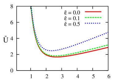
Figure 15: (color online). $\bar{U}$ as functions of $\bar{\theta}$ for a few values of $\bar{\epsilon}$.

IV.3 Distribution function of $\theta$

We combine (75) and (114). After setting $\mu=1$, we obtain

$$\Gamma\partial_{s}\theta=-\epsilon^{2}\frac{1}{4}-\frac{1}{2}\epsilon T^{2/3}-\frac{2\sqrt{6}-3}{4}T^{4/3}+\frac{24}{\theta^{4}}+\sqrt{2\Gamma T}\eta_{\theta},$$ (118)

where $\eta_{\theta}$ satisfies (77). Using the potential (116), we derive the $s$-stationary distribution function of $\theta$ as

$$P(\theta;T,\epsilon)=\frac{1}{Z_{\theta}}\exp\left(-\frac{U(\theta;T,\epsilon)}{T}\right),$$ (119)

where $Z_{\theta}$ is the normalization constant. It should be noted that the distribution function satisfies the scaling relation

$$P(\theta;T,\epsilon)=\bar{P}(\theta T^{1/3};\epsilon T^{-2/3}).$$ (120)

The expression (119) with (116) is the main result of our perturbative calculation.

Unfortunately, the distribution function (119) with (116) is not the precise expression even in the limit $\epsilon\ll T^{2/3}\ll 1$. There is a subtle reason. Recall that (118) is valid up to $O(\mu)$ in the formal expansion series. When we calculate higher order contributions in the equation for $\theta$, the coefficients in (118) are modified. For instance, $-\Gamma\Omega_{2}$ includes the contribution

$$I=-\frac{1}{2}\int_{-\infty}^{\infty}du(\partial_{u}\phi_{*}(u))F^{\prime\prime}_{u}(\phi_{*})\left\langle(\rho^{(1)})^{2}\right\rangle_{\rm\theta}.$$ (121)

By estimating this quantity, we have found that this term is $O(T^{4/3})+O(\epsilon^{2})+O(\epsilon T^{2/3})$. (See Appendix B.) The determination of the coefficients of these terms of $I$ is impossible without the numerical integration. Therefore, we did not derive the precise expression in the limit $\epsilon\ll T^{2/3}\ll 1$. Nevertheless, we present two positive remarks. First, terms of $O(T^{4/3})+O(\epsilon^{2})+O(\epsilon T^{2/3})$ do not appear beyond some order of expansion in $\mu$. Therefore, in principle, one may have the formula determining the coefficients of these terms. Second, the scaling relation (120) in the limit $\epsilon\ll T^{2/3}\ll 1$ seems valid up to all orders of expansion in $\mu$.

In order to check the validity of the scaling relation (120), we investigate the distribution function $P(\theta;T,\epsilon)$ for the case $\epsilon=0$ by numerical simulations of (1). In Fig. 16, we plotted $P(\theta;T,0)T^{-1/3}$ as functions of $\theta T^{1/3}$ for several values of $T$. One may find that four graphs for different values of $T$ are not completely collapsed on one curve in the region for small $\theta T^{1/3}$. However, since the two curves with $T=10^{-5}$ and $T=10^{-6}$ almost coincide with each other, we expect that one universal curve is obtained when $T$ is decreased further. We thus conjecture the scaling relation (120) in the limit $T\to 0$ is valid.

Furthermore, following our theory, we attempt to fit these numerical data by assuming the form

$$P(\theta;T,0)=\exp\left(-\frac{1}{T}\left[aT^{4/3}\theta+\frac{b}{\theta^{3}}\right]+c\right),$$ (122)

where $c$ is determined by the normalization condition when values of $a$ and $b$ are given. These values well-fitted to the numerical data are estimated as $a_{\rm fit}=0.36$ and $b_{\rm fit}=9$, which are compared with our theoretical values $a_{*}=(2\sqrt{6}-3)/4=0.4747\cdots$ and $b_{*}=8$. The slight difference between $(a_{\rm fit},b_{\rm fit})$ and $(a_{*},b_{*})$ comes from the contribution of higher order terms than $O(\mu)$. (As an example, the numerical estimation of $I$ in (121) provides $I\simeq 0.1T^{4/3}$, which might improve the difference between $a_{*}$ and $a_{\rm fit}$.)

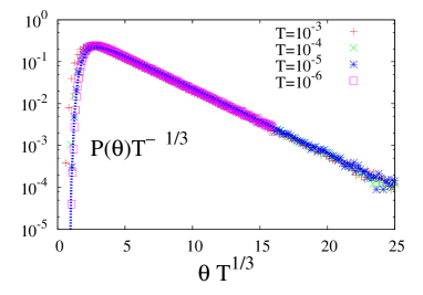
Figure 16: (color online). $P(\theta;T,0)T^{-1/3}$ as functions of $\theta T^{1/3}$ for several values of $T$. The dashed blue line represents the functional form (122) with $a=0.36$ and $b=9.0$.

IV.4 Results for the regime $T^{2/3}\ll\epsilon\ll 1$

The theoretical argument developed for the regime $\epsilon\ll T^{2/3}\ll 1$ cannot be applied to the regime $T^{2/3}\ll\epsilon\ll 1$, because a deviation $\rho(u)\simeq O(\epsilon T^{-1/3})$ becomes quite large there. (See (146) in Appendix B.) In particular, from a fact that the unperturbed potential $V_{\rm u}(\phi)$ goes back to the original potential $\tilde{V}_{T=0}$ in the extreme case $T=0$, it is obvious that we need to reformulate a perturbation theory.

The idea is natural and simple: we replace the unperturbative potential $V_{\rm u}(\phi)$ with a potential $W_{\rm u}(\phi)$ which is appropriate in this regime. Concretely, instead of (49) and (50), we define $\tilde{W}_{\epsilon}(\phi)$ by

$$F_{\epsilon,T=0}(\phi)=-\partial_{\phi}\tilde{W}_{\epsilon}(\phi),$$ (123)

where the functional form of $\tilde{W}_{\epsilon}(\phi)$ is given by

$$\tilde{W}_{\epsilon}(\phi)=-\frac{1}{4}\phi^{2}(\phi-1)^{4}-\frac{\phi^{2}}{4}\epsilon^{2}-\frac{\phi^{2}}{2}\left(\phi-1\right)^{2}\epsilon.$$ (124)

Here, $\tilde{W}_{\epsilon}(\phi)$ has two maximum points as displayed in Fig. 17.

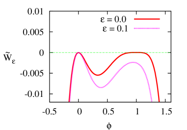
Figure 17: (color online). $\tilde{W}_{\epsilon}$ as functions of $\phi$. They possess two maxima at $\phi=0$ and $\phi=1-\epsilon/2$.

Then, in the manner similar to (51), we consider the decomposition

$$\tilde{W}_{\epsilon}(\phi)=W_{\rm u}(\phi)+\alpha(\phi),$$ (125)

where $\alpha(\phi)$ is chosen such that the two maximal values of the potential $W_{\rm u}(\phi)$ are identical. With this setting up, we study the equation

$$\partial_{s}\phi = \frac{1}{2}\partial_{t}^{2}{\phi}+\partial_{\phi}W_{\rm u}(\phi)-J_{T}(\phi)+\alpha_{\epsilon}^{\prime}(\phi)+\sqrt{2T}\eta.$$

After that, we repeat essentially the same procedures under the assumption that the last three terms are treated as perturbations. Note that the special solutions $\phi_{*}$ and $\phi_{\rm B}$ are redefined using $W_{\rm u}(\phi)$ instead of $V_{\rm u}(\phi)$. Then, in the regime $T^{2/3}\ll\epsilon\ll 1$, we derive the leading order expression

$$\Gamma\partial_{s}\theta=-\epsilon^{2}\frac{1}{4}+\frac{24}{\theta^{4}}+\sqrt{2\Gamma T}\eta_{\theta}.$$ (127)

Here, the complicated terms containing $\rho$ that appeared in the analysis in the regime $\epsilon\ll T^{2/3}\ll 1$ become higher order terms in the regime $T^{2/3}\ll\epsilon\ll 1$. Then, the $s$-stationary distribution function of $\theta$ is

$$P(\theta;T,\epsilon)=\frac{1}{Y}\exp\left(-\frac{1}{T}\left(\epsilon^{2}\frac{1}{4}\theta+\frac{8}{\theta^{3}}\right)\right),$$ (128)

where $Y$ is the normalization constant. Setting $\bar{\theta}=\epsilon^{1/2}\theta$ and $\bar{\epsilon}=\epsilon T^{-2/3}$, we rewrite $P(\theta;T,\epsilon)$ as $\bar{P}(\bar{\theta};\bar{\epsilon})$, where

$$\bar{P}(\bar{\theta};\bar{\epsilon})=\frac{1}{Y}\exp\left(-{\bar{\epsilon}}^{3/2}\left[\frac{1}{4}\bar{\theta}+\frac{8}{\bar{\theta}^{3}}\right]\right).$$ (129)

Since $\bar{\epsilon}\ll 1$, $\bar{P}(\bar{\theta};\bar{\epsilon})$ is further simplified to

$$\bar{P}(\bar{\theta};\bar{\epsilon})=\frac{1}{Y}\exp\left(-{\bar{\epsilon}}^{3/2}\left(\bar{\theta}-2(6^{1/4})\right)^{2}\frac{1}{4(6^{1/4})}\right).$$ (130)

This is equivalent to (27), where $\left\langle\theta\right\rangle$ and $\chi_{\rm\theta}$ are determined as

$$\left\langle\theta\right\rangle = 2(6^{1/4})\epsilon^{-1/2},$$ (131)

$$\chi_{\theta} = 2(6^{1/4})\epsilon^{-5/2}.$$ (132)

We expect that these expressions are exact in the limit $T^{2/3}\ll\epsilon\ll 1$. In Figs. 8 and 9, we display these theoretical results. They are in good agreement with the results of numerical simulations.

V Concluding remarks

In this paper, we have developed a theoretical framework for calculating statistical properties of critical fluctuations near a saddle-node bifurcation. The essential idea in our formulation is to choose an unperturbative state in accordance with the bifurcation structure. Since trajectories kinked in the time direction have much statistical weight near the bifurcation point, we express trajectories as $\phi(t)=\phi_{*}(t-\theta)+(\phi_{\rm B}(t)-\phi_{2})+\rho(t)$, where $\phi_{*}(t-\theta)$ represents a one-parameter family of classical solutions in the language of the path-integral expression. The parameter $\theta$ is regarded as a Goldstone mode associated with the time-translational symmetry. This expression naturally provides a divergent behavior, because the Goldstone mode is gapless or massless. Indeed, we have found that the fluctuation intensity of $\theta$ exhibits the divergence in the limit $\epsilon\to 0$ with small $T$ fixed and in the limit $T\to 0$ with $\epsilon=0$ fixed. The divergent behavior of $\chi_{\phi}(t)$ originates from critical fluctuations of $\theta$, and $\chi_{\phi}(t)$ becomes complicated due to a non-linear transformation to $\phi$ from $\theta$, as shown in Figs. 6 and 9.

Before ending the paper, we wish to explain how the results in this paper are related to understandings of other apparently different systems. First, our results suggest the following general story. When a saddle in a deterministic description becomes to be connected to an absorbing point at some parameter value, fluctuations of trajectories exhibit a critical divergence due to the existence of a Goldstone mode; and if the saddle is far from an absorbing point, the final value of the trajectory exhibits a discontinuity. Such cases might be related to a mixed order transition chi4_allstar1 ; chi4_allstar2 ; silbert_mix ; Toninelli_b ; toninelli ; schwartz ; sellitto . The elementary saddle-node bifurcation studied in this paper corresponds to the simplest one among them. As other types of bifurcation associated with a mixed order transition, we list up a saddle-connection bifurcation which arises in a model for a many-body colloidal system jstat ; epl , and a mode-coupling transition in a spherical $p$-spin glass model pspin_crisanti ; cugliandolo . Here, the important message of our paper is that one will be able to develop a calculation method for the statistical properties of critical fluctuations at a mixed order transition by applying the basic idea of our formulation to each system under investigation.

As an interesting and non-trivial, but still simple example of mixed order transition, we briefly discuss the mode-coupling transition of a spherical $p$-spin glass model with $p\geq 3$. The fluctuation property was studied by a mode-coupling equation supplemented with an external field franzparisi ; chi4_MCT or by the field theoretical analysis chi4_BB . Differently from these previous methods, we will be able to consider another theoretical framework for critical fluctuations along with the above-mentioned strategy. Concretely, we start with a useful expression of trajectories as we did. In the thermodynamic limit, the equation for the time-correlation function obeys a mode-coupling equation pspin_crisanti ; cugliandolo , and recently we have derived a global expression of the solution near the mode-coupling transition pspin , which is similar to (12). From this result, we may express a fluctuating correlator in terms of a Goldstone mode $\lambda$ associated with the dilation symmetry that arises in the slowest time scale. Thus, it is natural to describe critical fluctuations near the mode-coupling transition in terms of fluctuations of $\lambda$. The concrete calculation will be reported in future.

The results in this paper also provide some physical insights into the dynamics associated with a mixed order transition even if the calculation has never been performed yet. For example, let us consider a dynamical behavior of a super-cooled liquid cavagna . Within a framework of the mode-coupling theory, a mode-coupling transition occurs at some temperature or density Gotze . In some super-cooled liquids, the behavior associated with the transition has been observed approximately kob ; megen . The physical picture is well-understood: when the system is near the mode-coupling transition point, a particle cannot move freely; and only when the particle gets over surrounding particles, it can move. Such an event is called an unlocking event chi4_BB or a bond breakage event ryamamoto . As the mode-coupling transition is approached, the frequency of unlocking events becomes smaller and the events become correlated more and more in a spatially heterogeneous manner, which is called the dynamical heterogeneity. (See Refs. chi4_allstar1 ; chi4_allstar2 as reviews, and Refs. ediger ; durian ; shear ; dh_re_berthier as experimental studies, and Refs. ryamamoto ; dh_harrowell ; dh_parisi ; early1 ; dh_glotzer ; dh_glotzer2 ; dh_berthier ; chi4_lacevic ; silbert_mix ; sellitto as numerical observations, and Refs. schwartz ; franzparisi ; chi4_theory1 ; chi4_BB ; chi4_MCT ; garrahan ; WBG ; Toninelli_b ; toninelli ; theory_review as theoretical studies.)

From our point of view, we conjecture that an unlocking event near the mode-coupling transition might correspond to an exiting event from a marginal saddle in some local dynamics. Then, the results of our paper suggest that the most important characterization of the dynamical heterogeneity is space-time fluctuations of exiting time from a saddle-point. At present, it seems difficult to derive such local dynamics theoretically, but it is tempting to connect the idea of cooperative arrangement regions to a marginal saddle in some local dynamics. Since the distribution function of exiting time from cooperative arrangement regions exhibits an interesting behavior matsui , the theoretical derivation of the observation may be a good starting point for the consideration. The final goal in this direction is to obtain a simple expression determining space-time fluctuations of the Goldstone mode on the basis of a microscopic particle model. We will study it step by step toward this goal.

Related to the description of dynamical heterogeneity, we remark on a well-recognized conjecture that the mode-coupling transition described theoretically is nothing but a cross-over phenomenon in finite dimensional systems. In order to understand the nature of this cross-over, one needs to describe an activation process from “pseudo” meta-stable states which are not defined clearly, but might be connected to that defined in the mean-field approximation. Although, physically, the activation process corresponds to a nucleation of some domain, its mathematical expression is highly non-trivial. Here, when we apply our analysis to a finite dimensional system, in our viewpoint, the cross-over phenomenon is equivalent to the finite value of the expectation of the Goldstone mode. Thus, we have only to calculate an asymptotic tail of the effective potential for the Goldstone mode in the limit $t\to\infty$. Since the analysis of the super-cooled liquid is too difficult, we should begin with the study of a diffusively coupled model of local dynamics (1) with (2). (See Ref. 1dimlett as a report on a numerical experiment with $\epsilon=0$.) It would be possible to develop the mean-field analysis of the spatially extended system, but it seems difficult to treat spatial fluctuations accurately even for such a simple system. To develop a systematic theory beyond the mean field analysis is a challenging problem.

Finally, let us recall that our formulation is based on the fictitious time formalism. One may expect that the calculation can be done within a standard Martin-Siggia-Rose (MSR) formalism msr . Such a reformulation is particularly important when we study more complicated systems. In this context, it is worthwhile noting that the third term in (116) has been obtained in the MSR formulation with a semi-classical approximation fukui . Such calculation techniques in spatially extended systems will be developed in future.

Appendix A Path integral expression

We derive the path-integral expression (5) with (6) from the Langevin equation (1) with (3). In particular, we carefully discuss the derivation of the so-called Jacobian term.

Let $\Delta t$ be a sufficiently small time interval. We discretize (1) as

$$\phi_{n}-\phi_{n-1} = [f_{\epsilon}(\phi_{n-1})+f_{\epsilon}(\phi_{n})]\frac{\Delta t}{2}$$ (133)

$$+\xi_{n-1}\Delta t+O((\Delta t)^{2}),$$

with $n=1,2,\cdots,N$. Here, $\left(\xi_{n}\right)_{n=0}^{N-1}$ obeys the Gaussian distribution

$$P_{\xi}(\xi_{0},\xi_{1},\cdots,\xi_{N-1})=\left(\frac{\Delta t}{4\pi T}\right)^{N/2}\exp\left(-\frac{\Delta t}{4T}\sum_{n=0}^{N-1}\xi_{n}^{2}\right).$$

In the limit $\Delta t\to 0$, $\phi_{n}$ is expected to provide $\phi(n\Delta t)$ in the Langevin equation.

Let us fix $\phi_{0}$. Then, a sequence $(\xi_{0},\xi_{1},\cdots,\xi_{N-1})$ determines uniquely the sequence $(\phi_{1},\cdots,\phi_{N})$. Thus, the distribution function of the sequence $(\phi_{n})_{n=1}^{N}$ is expressed as

$$P(\phi_{1},\cdots,\phi_{N})=P_{\xi}(\xi_{0},\cdots,\xi_{N-1})\left|\frac{\partial(\xi_{0},\cdots,\xi_{N-1})}{\partial(\phi_{1},\cdots,\phi_{N})}\right|.$$

Here, the determinant of the Jacobian matrix is calculated as

$$\left|\frac{\partial(\xi_{0},\cdots,\xi_{N-1})}{\partial(\phi_{1},\cdots,\phi_{N})}\right|=\prod_{n=1}^{N}\left|1-\frac{1}{2}f_{\epsilon}^{\prime}(\phi_{n})\Delta t\right|\frac{1}{(\Delta t)^{N}}.$$ (136)

By using the relation

$$\prod_{n=1}^{N}\left|1-\frac{1}{2}f_{\epsilon}^{\prime}(\phi_{n})\Delta t\right|$$ (137)

$$= 1-\sum_{n=1}^{N}\frac{1}{2}f_{\epsilon}^{\prime}(\phi_{n})\Delta t+O((\Delta t)^{2})$$

$$= \exp\left(-\sum_{n=1}^{N}\frac{1}{2}f_{\epsilon}^{\prime}(\phi_{n})\Delta t+O((\Delta t)^{2})\right),$$

we obtain

$$P(\phi_{1},\cdots,\phi_{N})=\left(\frac{1}{4\pi T\Delta t}\right)^{N/2}$$

$$\exp\left(-\frac{\Delta t}{4T}\sum_{n=1}^{N}\left\{\right.\right.$$

$$\left.\left[\frac{\phi_{n}-\phi_{n-1}}{\Delta t}-(f_{\epsilon}(\phi_{n-1})+f_{\epsilon}(\phi_{n}))/2\right]^{2}\right.$$

$$\left.\left.+2Tf_{\epsilon}^{\prime}(\phi_{n})+O((\Delta t)^{1/2})\right\}\right).$$ (138)

By taking the limit $\Delta t\to 0$ and $N\to\infty$ with $N\Delta t$ fix, we write formally (5) with (6).

At the end of this appendix, we remark on a discretization method. One may notice that another discretized expression

$$\phi_{n}-\phi_{n-1}=f_{\epsilon}(\phi_{n-1})\Delta t+\xi_{n-1}\Delta t+O((\Delta t)^{3/2})$$ (139)

does not yield the Jacobian term, because in this case the determinant of the Jacobian matrix

$$\left|\frac{\partial(\xi_{0},\cdots,\xi_{N-1})}{\partial(\phi_{1},\cdots,\phi_{N})}\right|=\frac{1}{(\Delta t)^{N}}$$ (140)

does not depend on $\phi$. However, the discretization (139) provides

$$P(\phi_{1},\cdots,\phi_{N})=\frac{1}{(\Delta t)^{N}}\left(\frac{\Delta t}{4\pi T}\right)^{N/2}$$

$$\exp\left(-\frac{\Delta t}{4T}\sum_{n=1}^{N}\right.$$

$$\left.\left\{\left[\frac{\phi_{n}-\phi_{n-1}}{\Delta t}-f_{\epsilon}(\phi_{n-1})\right]^{2}+R\right\}\right),$$ (141)

where the term $R$ comes from the product of $\phi_{n}-\phi_{n-1}$ and the last term $O((\Delta t)^{3/2})$ in the right-hand side of (A7) when $\xi_{n-1}^{2}$ is evaluated. Explicitly, $R$ is equal to $O((\Delta t)^{3/2})(\phi_{n}-\phi_{n-1})/(\Delta t)^{2}$. We here note that $\phi_{n}-\phi_{n-1}\simeq O((\Delta t)^{1/2})$. This leads to $R=O((\Delta t)^{0})=O(1)$ in the limit $\Delta t\to 0$. Therefore, (141) is not useful in the limit $\Delta t\to 0$. With regard to the discretization problem, we remark that numerical simulations of the discretized form (139) yield (22) and (23), too. Here, one may confirm that (22) and (23) cannot be obtained without the Jacobian term in (6) within the analysis of the path integral expression. Therefore, this example provides an evidence for the claim that the path integral expression in the limit $\Delta t\to 0$ always contains the last term in (6).

Appendix B estimation of $I$

We estimate the integral $I$ given in (121). Before the estimation, we need to evaluate $\rho^{(1)}$. We multiply by $\Phi_{\lambda}^{*}(u)$ on both sides of (89) and integrate them over $-\infty\leq u\leq\infty$. We then consider the $s$-stationary state and extract the lowest order terms. By using (67), we derive

$$\lambda\left\langle\psi_{\lambda}^{(1)}\right\rangle_{\theta} = -\frac{1}{2}\int_{-\infty}^{\infty}du\Phi_{\lambda}^{*}(u)F_{\rm u}^{\prime\prime}(\phi_{*}(u))\left\langle\left(\rho^{(1/2)}\right)^{2}\right\rangle_{\theta}$$ (142)

$$-\int_{-\infty}^{\infty}du\Phi_{\lambda}^{*}(u)G_{\epsilon}(\phi_{*}(u)),$$

where the contribution from the fourth and fifth terms in the right hand side of (89) have been neglected, because they are estimated as higher order terms. From (67), (81), and (82), we obtain

$$\left\langle\rho^{(1)}(u)\right\rangle_{\theta} = -\frac{T}{2}\int_{-\infty}^{\infty}dvG(u,v)F_{\rm u}^{\prime\prime}(\phi_{*}(v))G(v,v)$$ (143)

$$+\int_{-\infty}^{\infty}dvG(u,v)G_{\epsilon}(\phi_{*}(v)).$$

Since the most singular behavior arises around $u\to-\infty$, we estimate $\left\langle\rho^{(1)}(u)\right\rangle$ in the limit $u\to-\infty$ by noting (88). The first term in (143) is estimated as $T\xi\times 1/m_{-}\times F^{\prime\prime}_{0}\times 1/m_{-}$, where $\xi$ is the length scale over which the integral is dominant. By using $\xi\sim 1/m_{-}\sim O(T^{-1/3})$ (see (86)), we estimate the first term of (143) as

$$-\frac{T}{2}\int_{-\infty}^{\infty}dvG(u,v)F_{\rm u}^{\prime\prime}(\phi_{*}(v))G(v,v)$$ (144)

$$\simeq O\left(T\times T^{-1/3}\times T^{-1/3}\times T^{1/3}\times T^{-1/3}\right)$$

$$\simeq O\left(T^{1/3}\right).$$

Similarly, the second term in (143) is estimated as

$$\int_{-\infty}^{\infty}dvG(u,v)G_{\epsilon}(\phi_{*}(v))$$ (145)

$$\simeq \xi\times 1/m_{-}\times G_{\epsilon}(\phi_{*}(u))$$

$$\simeq O\left(T^{-1/3}\times T^{-1/3}\times\epsilon T^{1/3}\right)$$

$$\simeq O\left(\epsilon T^{-1/3}\right).$$

Thus, we write

$$\left\langle\rho^{(1)}(u\to-\infty)\right\rangle_{\theta}=O(T^{1/3})+O(\epsilon T^{-1/3}).$$ (146)

From this result, the quantity $I$ in (121) is estimated as follows. First, (121) is rewritten as

$$I = -\frac{1}{2}\int_{-\phi_{2}}^{\phi_{1}}d\phi_{*}F^{\prime\prime}_{u}(\phi_{*})\left\langle\rho^{(1)}(u(\phi_{*}))\right\rangle^{2}_{\theta},$$ (147)

where $u(\phi_{*})$ is the inverse function of $\phi_{*}(u)$. In this integration, the most dominant contribution arises from the integral region $[-\phi_{2},1]$, and this contribution is estimated as

$$I \simeq O\left(T^{1/3}\times T^{1/3}\times(T^{1/3}+\epsilon T^{-1/3})^{2}\right)$$ (148)

$$\simeq O(T^{4/3})+O(\epsilon T^{2/3})+O(\epsilon^{2}).$$

References

- (1) N. Goldenfeld, Lectures on Phase Transitions and the Renormalization Group, (Addison-Wesley, New York, 1992).
- (2) Y. Kuramoto, Chemical Oscillations, Waves, and Turbulence, (Springer, Berlin, 1984).
- (3) M. A. Munoz, Advances in Condensed Matter and Statistical Physics, ed. E. Korutcheva and R. Cuerno, (Nova Science Publishers, New York, 2004), 37 (2004).
- (4) J. Guckenheimer and P. Holmes, Nonlinear Oscillations, Dynamical Systems and Bifurcations of Vector Fields (Springer-Verlag, New York, 1983).
- (5) K. Binder, Phys. Rev. B 8, 3423 (1973).
- (6) P. Reimann, C. Van den Broeck, H. Linke, P. Hänggi, J. M. Rubi, and A. Perez-Madrid, Phys. Rev. E 65, 031104 (2002).
- (7) J. J. Tyson, K. C. Chen, and B. Novak, Current Opinion in Cell Biology 15, 221 (2003).
- (8) B. Lindner, A. Longtin, and A. Bulsara, Neural Computation 15, 1761 (2003).
- (9) H. Ohta and S. Sasa, Phys. Rev. E 78, 065101(R) (2008).
- (10) P. B. Warren, Phys. Rev. E 80, 030903(R) (2009).
- (11) M. Iwata and S. Sasa, J. Phys. A: Math. Theor. 42, 075005 (2009).
- (12) H. Ohta and S Sasa, arXiv:0912.4790.
- (13) M. Iwata and S. Sasa, Phys. Rev. E 78, 055202(R) (2008).
- (14) R. Kubo, K. Matsuo, and K. Kitahara, J. Stat. Phys. 9, 51 (1973).
- (15) L. Berthier, G. Biroli, J. P. Bouchaud, W. Kob, K. Miyazaki, and D. R. Reichman, J. Chem. Phys. 126, 184503 (2007).
- (16) L. Berthier, G. Biroli, J. P. Bouchaud, W. Kob, K. Miyazaki, and D. R. Reichman, J. Chem. Phys. 126, 184504 (2007).
- (17) C. S. O’Hern, L. E. Silbert, A. J. Liu, and S. R. Nagel, Phys. Rev. E 68, 011306 (2003).
- (18) M. Sellitto, G. Biroli, and C. Toninelli, Europhys. Lett. 69, 496 (2005).
- (19) J. M. Schwarz, A. J. Liu, and L. Q. Chayes, Europhys. Lett. 73, 560 (2006).
- (20) C. Toninelli, G. Biroli, and D. S. Fisher, Phys. Rev. Lett. 96, 035702 (2006).
- (21) C. Toninelli and G. Biroli, J. Stat. Phys. 130, 83 (2008).
- (22) A. Greiner, W. Strittmatter, and J. Honerkamp, J. Stat. Phys 51, 95 (1988).
- (23) C. W. Gardiner, Handbook of Stochastic Methods: for Physics, Chemistry and the Natural Sciences (Springer Series in Synergetics) 3rd. ed., (Springer, Berlin, 2004).
- (24) G. Parisi and W. Yongshi, Sci. Sin. 24, 483 (1981).
- (25) K. Kawasaki and T. Ohta, Physica A 116, 573 (1982).
- (26) S. Ei and T. Ohta, Phys. Rev. E 50, 4672 (1994).
- (27) G. Costantini and F. Marchesoni, Phys. Rev. Lett. 87, 114102 (2001).
- (28) Y. Kuramoto, Prog. Theor. Phys. Suppl. 99, 244 (1989).
- (29) M. C. Cross and P. C. Hohenberg, Rev. Mod. Phys. 65, 851 (1993).
- (30) M. Iwata and S. Sasa, J. Stat. Mech. L10003 (2006).
- (31) M. Iwata and S. Sasa, Europhys. Lett. 77, 50008 (2007).
- (32) A. Crisanti, H. Horner, and H. J. Sommers, Z. Phys. B 92, 257 (1993).
- (33) L. F. Cugliandolo and J. Kurchan, Phys. Rev. Lett. 71, 173 (1993).
- (34) S. Franz and G. Parisi, J. Phys. Condens. Matter 12, 6335 (2000).
- (35) G. Biroli, J. P. Bouchaud, K. Miyazaki, and D. R. Reichman, Phys. Rev. Lett. 97, 195701 (2006).
- (36) G. Biroli and J. P. Bouchaud, Europhys. Lett. 67, 21 (2004).
- (37) M. Iwata and S. Sasa, J. Phys. A: Math. Theor. 42, 245001 (2009).
- (38) A. Cavagna, Physics Reports 476, 51 (2009).
- (39) W. Götze, Liquids, Freezing and Glass Transition, ed D. Levesque et al (Elsevier, New York, 1991).
- (40) W. Kob, Slow Relaxations and Nonequilibrium Dynamics in Condensed Matter (Les Houches 2002 Session LXXVII) , ed J. L. Barrat et al (Berlin: Springer, 2003), 199 (2003).
- (41) W. V. Megen and S. M. Underwood, Phys. Rev. Lett. 70, 2766 (1993).
- (42) R. Yamamoto and A. Onuki, Phys. Rev. E 58, 3515 (1998).
- (43) M. D. Ediger, Ann. Rev. Phys. Chem. 51, 99 (2000).
- (44) O. Dauchot, G. Marty, and G. Biroli, Phys. Rev. Lett. 95, 265701 (2005).
- (45) L. Berthier, G. Biroli, J. P. Bouchaud, L. Cipelletti, D. El Masri, D. L’Hôte, F. Ladieu, and M. Pierno, Science 310, 1797 (2005).
- (46) A. Abate and D. Durian, Phys. Rev. E 74, 031308 (2006).
- (47) S. Butler and P. Harrowell, J. Chem. Phys. 95, 4454 (1991).
- (48) M. Hurley and P. Harrowell, Phys. Rev. E 52, 1694 (1995).
- (49) G. Parisi, J. Phys. Chem. B 103, 4128 (1999).
- (50) C. Bennemann, C. Donati, J. Bashnagel, and S. C. Glotzer, Nature (London) 399, 246 (1999).
- (51) S. C. Glotzer, J. Non-Cryst. Solids 274, 342 (2000).
- (52) N. Lačević, F. W. Starr, T. B. Schrøder, and S. C. Glotzer, J. Chem. Phys. 119, 7372 (2003).
- (53) L. Berthier, Phys. Rev. E 69, 020201(R) (2004).
- (54) C. Donati, S. Franz, G. Parisi, and S. C. Glotzer, J. Non-Cryst. Solids 307, 215 (2002).
- (55) S. Whitelam, L. Berthier, and J. P. Garraham, Phys. Rev. Lett. 92, 185705 (2004).
- (56) C. Toninelli, M. Wyart, L. Berthier, G. Biroli, and J. P. Bouchaud, Phys. Rev. E 71, 041505 (2005).
- (57) A. C. Pan, J. P. Garrahan, and D. Chandler, Phys. Rev. E 72, 041106 (2005).
- (58) J. Matsui, private communication.
- (59) P. C. Martin, E. D. Siggia, and H. A. Rose, Phys. Rev. A 8, 423 (1973).
- (60) T. Fukui, private communication.