b-Jet Identification in the D0 Experiment

Abstract

Algorithms distinguishing jets originating from $b$ quarks from other jet flavors are important tools in the physics program of the D0 experiment at the Fermilab Tevatron $p\bar{p}$ collider. This article describes the methods that have been used to identify $b$-quark jets, exploiting in particular the long lifetimes of $b$-flavored hadrons, and the calibration of the performance of these algorithms based on collider data.

FERMILAB-PUB-10-037-E

1 Introduction

The bottom quark occupies a special place among the fundamental fermions: on the one hand, its mass (of the order of 5 GeV [1]) is substantially larger than that of the (next lightest) charm quark. On the other hand, it is light enough to be produced copiously at present-day high energy colliders.

In particular, unlike the top quark, the bottom quark is lighter than the $W$ boson, preventing decays to on-shell $W$ bosons. As a result, it lives long enough for hadronization to occur before its decay. The average lifetime of $b$-flavored hadrons (referred to as $b$ hadrons in the following) has been measured to be about 1.5 ps [1]: this is sufficiently long for $b$ hadrons, even of moderate momentum, to travel distances of the order of at least a mm. Combined with the relatively large mass of $b$ hadrons, the use of precise tracking information allows the detection of the presence of $b$ hadrons through their charged decay products. In addition, $b$ hadron decays often lead to the production of high momentum leptons; especially at hadron colliders, the observation of such leptons provides easy access to samples with enhanced $b$-jet content. The identification of jets originating from the hadronization of bottom quarks (referred to as $b$-jet identification or $b$-tagging in the following) in the D0 experiment is the subject of this publication.

1.1 The upgraded D0 detector

The D0 experiment is one of the two experiments operating at the Tevatron $p\bar{p}$ Collider at Fermilab. After a successful Tevatron Run I, which led to the discovery of the top quark [2, 3], the Tevatron was upgraded to provide both a higher center-of-mass energy (from 1.8 TeV to 1.96 TeV) and a significant increase in luminosity. Run II started in 2001, and the Tevatron delivered 1.6 fb^-1 of integrated luminosity to the experiments by March 2006, at which time another detector upgrade was commissioned. This publication refers to the Run II data taken before March 2006, commonly denoted as the Run IIa period.

To cope with the increased luminosity and decreased bunch spacing (from 3.6 $\mu$s to 396 ns) in Run II, the D0 detector also underwent a significant upgrade, described in detail elsewhere [4]. In particular, a 2 T central solenoid was installed to provide an axial magnetic field used to measure the momentum of charged particles. Correspondingly, the existing tracking detectors were removed and replaced with two new detectors, shown in Fig. 1:

• the central fiber tracker (CFT), consisting of about 77,000 axial and small-angle stereo scintillating fibers arranged in eight concentric layers, and covering the pseudorapidity region $|\eta|\lesssim 1.7$;

• and the silicon microstrip tracker (SMT) [5], a detector featuring 912 silicon strip sensor modules arranged in six barrel and sixteen disk structures, allowing tracking up to $|\eta|\lesssim 3$. Of particular interest is the innermost layer of SMT barrel sensors: its proximity to the beam line (at a radius of 2.7 cm) results in a relatively small uncertainty in the extrapolation of tracks to the beam line, and hence in good vertex reconstruction capabilities.

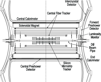
Figure 1: The Run IIa central tracking detectors.

The ability to identify efficiently the $b$ quarks in an event considerably broadens the range of physics topics that can be studied by the D0 experiment in Run II. While the analysis leading to the observation of the top quark by D0 in Run I employed only semimuonic decays $b\rightarrow\mu X$, the use of lifetime tagging allows for a more precise determination of the top quark properties (see e.g. [6]). The search for electroweak production of top quarks ($p\bar{p}\to tb+X,tqb+X$) relies heavily as well on the efficiency to identify $b$ jets and reject light and $c$ jets, as demonstrated in the recent observation of this production process [7]. The search for the standard model Higgs boson also depends on $b$-jet identification: a relatively light ($m_{H}\lesssim 135\mbox{ GeV}$) Higgs boson will decay predominantly to $b\bar{b}$ quark pairs. Finally, various regions of the minimal supersymmetric standard model parameter space lead to final states containing $b$ quarks (from gluino or stop quark decays), and efficient $b$ tagging greatly increases the sensitivity of the search for those final states.

This article is subdivided as follows. Section 2 describes the objects that serve as input to the $b$-tagging algorithms. Section 3 introduces the steps taken before applying the tagging algorithms proper. Sections 4, 5, and 6 describe the basic ways in which lifetime-correlated variables are extracted. Section 7 describes the combination of these variables in an artificial neural network to obtain an optimal tagging performance. Finally, Sections 8 and 9 detail how Tevatron data are used to calibrate the performance of the resulting tagging algorithm.

2 Object Reconstruction

Besides the charged particle tracks, which are reconstructed from hits (clustered energy deposits) in the CFT and SMT detectors, the input for lifetime identification of $b$-quark jets consists of two kinds of reconstructed objects:

• primary vertices, which are built from two or more charged particle tracks that originate from a common point in space;

• hadron jets, which are reconstructed primarily from their energy deposition in the calorimeter.

These objects are described below.

2.1 Primary vertex reconstruction

The knowledge of the $p\bar{p}$ interaction point or primary vertex of an interaction is important to provide the most precise reference point for the lifetime-based tagging algorithms described in subsequent sections. In addition, multiple interactions can occur during a single bunch crossing. It is therefore necessary to select the primary vertex associated to the interaction of interest. The reconstruction and identification of the primary vertex at D0 consists of the following steps: (i) track selection; (ii) vertex fitting using a Kalman filter algorithm to obtain a list of candidate vertices; (iii) a second vertex fitting iteration using an adaptive algorithm to reduce the effect of outlier tracks; and (iv) primary vertex selection.

In the first stage, tracks are selected if their momentum component in the plane perpendicular to the beam line, $p_{T}$, exceeds 0.5 GeV, and they have two or more hits in the SMT (counted as the number of hit ladders or disks) if the track is within the SMT geometric acceptance as measured in the $(\eta,z)$ plane. The selected tracks are then clustered along the $z$ direction in 2 cm regions to separate groups of tracks coming from different interactions, as evidenced by the tracks’ $z$ coordinates at their distance of closest approach to the beam line.

In the second stage, the tracks in each of the $z$ clusters are used to reconstruct a vertex. This is done in two passes. In the first pass, the selected tracks in each cluster are fitted to a common vertex. A Kalman filter vertex fitter is used for this step where tracks with the highest $\chi^{2}$ contribution to the vertex are removed in turn, until the total vertex $\chi^{2}$ per degree of freedom is less than 10. In the second pass, the track selection in each $z$ cluster is refined based on the track’s distance of closest approach in the transverse plane, $d$, to the vertex position computed in the first pass, as well on its uncertainty $\sigma_{d}$: only tracks with impact parameter significance $\mathcal{S}_{d}\equiv d/\sigma_{d}$ satisfying $|\mathcal{S}_{d}|<5$ are retained.

Once the outliers with respect to the beam position have been removed from the selected tracks, an adaptive vertex algorithm [8, 9] is used to fit the selected tracks to a common vertex in each cluster. This algorithm differs from the Kalman filter vertex fitter in that all tracks remaining after the Kalman filter selection procedure are allowed to contribute to the final vertex fit instead of rejecting those tracks whose $\chi^{2}$ contribution to the vertex fit exceeds a certain value. It is especially suited to reducing the contribution of distant tracks to the vertex fit, thus obtaining a better separation between primary and secondary vertices. The algorithm proceeds in three iterative stages: (i) the track candidates in a $z$-cluster are fitted using a Kalman filter; (ii) each track is weighted according to its $\chi^{2}$ contribution to the vertex found in the previous step, and if the weight is less than $10^{-6}$, the track is eliminated; and (iii) steps (i) and (ii) are repeated until either the weights converge (the maximum change in track weights between consecutive iterations is less than $10^{-3}$) or more than 100 iterations have been performed.

The weights are adapted in each iteration: a track $i$ associated with a small weight in one iteration will affect the weights of all other tracks in the next iteration because they are derived with respect to the new vertex position obtained with a down-weighted contribution from track $i$. The tracks are weighted in step ii) according to their $\chi^{2}$ contribution to the vertex by a sigmoidal function:

$$w_{i}=\frac{1}{1+e^{(\chi^{2}_{i}-\chi^{2}_{\mbox{\scriptsize cutoff}})/2T}}.$$ (1)

Here, $\chi^{2}_{i}$ is the $\chi^{2}$ contribution of track $i$ to the vertex; $\chi^{2}_{\mbox{\scriptsize cutoff}}$ is the $\chi^{2}$ value at which the weight function drops to 0.5; and $T$, like the temperature in the Fermi function in statistical thermodynamics, is a parameter that controls the sharpness of the function. Figure 2 shows the weight function used at D0 with $\chi^{2}_{\mbox{\scriptsize cutoff}}=4$ and $T=1$.

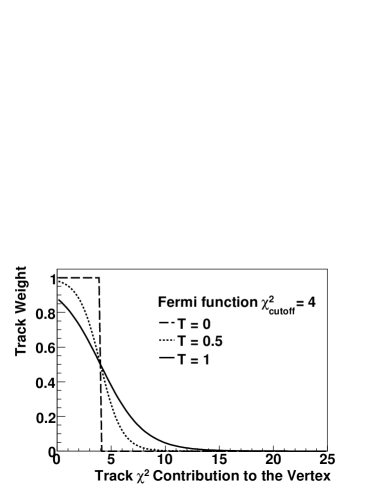
Figure 2: Weight given to tracks as a function of the $\chi^{2}$ distance to the vertex for different T parameters. In the adaptive fitting, all tracks contribute to the fit when $T>0$. The value used in the reconstruction algorithm is $T=1$.

Once all possible vertices in the event are accurately reconstructed, the fourth and final step consists of selecting which of the fitted vertices is the result of the hard scatter interaction. The hard scatter vertex is distinguished from soft-interaction vertices by the higher average $p_{T}$ of its tracks, as shown in Fig. 3. The probability $\mathcal{P}_{\mbox{\scriptsize MB}}^{\mbox{\scriptsize trk}}(p_{T})$ that the observed $p_{T}$ of a given track is compatible with the track originating from a soft interaction is computed as

$$\mathcal{P}_{\mbox{\scriptsize MB}}^{\mbox{\scriptsize trk}}(p_{T})=\frac{\int_{p_{T}}^{\infty}\mathcal{F}(p_{T}^{\prime})dp_{T}^{\prime}}{\int_{p_{T}^{\min}}^{\infty}\mathcal{F}(p_{T}^{\prime})dp_{T}^{\prime}}.$$ (2)

Here, $\mathcal{F}(p_{T})$ is the $p_{T}$ distribution of tracks attached to soft interaction vertices in $Z\rightarrow\mu^{+}\mu^{-}$ candidate events requesting that they be separated from the $Z\rightarrow\mu^{+}\mu^{-}$ interaction vertex by more than 10 cm. $\mathcal{F}(p_{T})$ is depicted in Fig. 3a. Only tracks with $p_{T}>p_{T}^{\min}=0.5\mbox{ GeV}$ are used in this calculation. For each reconstructed vertex, the probability that it is consistent with a minimum bias interaction is formed as

$$\mathcal{P}_{\mbox{\scriptsize MB}}^{\mbox{\scriptsize vtx}} = \Pi\cdot\sum_{j=0}^{N_{\mbox{\scriptsize trk}}-1}\frac{(-\ln\Pi)^{j}}{j!}\;\;\;\mbox{with}\;\;\;$$ (3)

$$\Pi = \prod_{i=1}^{N_{\mbox{\scriptsize trk}}}\mathcal{P}_{\mbox{\scriptsize MB}}^{\mbox{\scriptsize trk}}(p_{T,i})\;,$$

where $N_{\mbox{\scriptsize trk}}$ is the number of tracks attached to the vertex; a motivation for this expression is provided in Sec. 5. The selected primary vertex is the one with the lowest $\mathcal{P}_{\mbox{\scriptsize MB}}^{\mbox{\scriptsize vtx}}$; the resulting $\mathcal{P}_{\mbox{\scriptsize MB}}^{\mbox{\scriptsize vtx}}$ distribution is shown in Fig. 3b.

The reconstruction and identification efficiency in data is between 97% and 100% for primary vertices reconstructed up to $|z|$ = 100 cm, as measured on the $Z\rightarrow\mu^{+}\mu^{-}$ candidate event sample. For multijet events, the position resolution of the selected primary vertex in the transverse plane can be determined by subtracting the known beam width quadratically from the width of the observed vertex position distribution. This resolution improves with increasing track multiplicity and is better than the beam width (around 30 $\mu$m) for events with at least 10 tracks attached to the primary vertex.

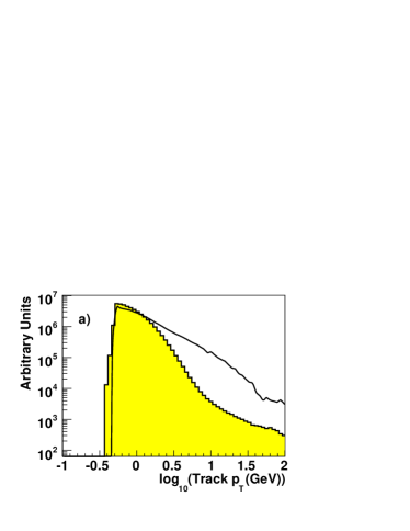
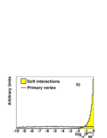
Figure 3: (a): The track $p_{T}$ spectrum for soft-interaction vertices in the D0 data selected as described in the text. For comparison, the corresponding distribution is also shown for the primary vertices in one data run selected on the basis of their $\mathcal{P}_{\mbox{\scriptsize MB}}^{\mbox{\scriptsize vtx}}$ values, as also described in the text. The soft-interaction vertex distribution is $\mathcal{F}(p_{T})$ in Eq. 2. (b): The $\mathcal{P}_{\mbox{\scriptsize MB}}^{\mbox{\scriptsize vtx}}$ distribution for soft-interaction vertices and multijet (hard scatter) primary vertices.

2.2 Jet reconstruction and calibration

The vast majority of data analyses in D0 make use of so-called cone jets, which collect all calorimeter energy deposits within a fixed angular distance $\mathcal{R}\equiv\sqrt{(\Delta y)^{2}+(\Delta\phi)^{2}}$ in ($y$,$\phi$) space. Specifically, the cone jet reconstruction algorithm used within D0 is the Run II cone jet algorithm [10]. This algorithm is insensitive to the presence of soft or collinear radiation off partons, thus allowing for detailed comparisons of jet distributions in the D0 data with theoretical predictions. The cone radii used in analyses in D0 are $\mathcal{R}=0.5$ and $\mathcal{R}=0.7$, but for most high $p_{T}$ physics the $\mathcal{R}=0.5$ cone jets are used. It is only these jets that are described in this article.

As the jets are reconstructed on the basis of calorimetric information, comparisons between the data and jets simulated using Monte Carlo (MC) methods require corrections for various effects:

• energy deposits not from the hard interaction (either from the remnant of the original $p\bar{p}$ system or from additional soft interactions or noise);

• the (energy dependent) calorimeter response to incident high-energy particles;

• the net energy flow through the jet cone because of the finite size of showers in the calorimeter and the bending of charged particle trajectories by the magnetic field.

The topic of the determination of the jet energy scale (JES) is described in a separate paper [11]. The resulting JES, by itself, does not yet account for neutrinos from decays of $b$- or $c$-flavored hadrons escaping undetected. While such additional corrections may be important for physics analyses, $b$ tagging is only sensitive to it because the tagging performance obtained in data (Sec. 8) is parametrized in terms of jet $p_{T}$ (and $\eta$) and applied to simulated jets. For this purpose, corrections for undetected neutrinos (and for the energy not deposited in the calorimeter, in the case of muons associated with jets) do not need to be applied, provided that data and simulated jets are treated identically.

3 Tagging Prerequisites

In order to evaluate the performance of the $b$-tagging algorithms described in the following sections, it is necessary to define properly the meaning of “$b$ jet”. Also, several steps are carried out before proceeding with the tagging proper. These steps are discussed below.

3.1 Flavor assignment in simulated events

The $b$-tagging algorithms used within the D0 experiment are jet based rather than event based. This choice makes sense especially for high-luminosity hadron colliders, where pile-up (overlapping electronics signals) from previous interactions, as well as multiple interactions in the same bunch crossing, may lead to other reconstructed tracks and jets in the event besides those of the “interesting” high-$p_{T}$ interaction.

However, this choice introduces an ambiguity for jets in simulated events: In order to estimate the performance of a $b$-tagging algorithm, it is first necessary to specify precisely how a jet’s flavor is determined. The following choice has been made:

• if at the particle level (i.e., after the hadronization of the partonic final state), a hadron containing a $b$ quark (denoted in the following as $b$ hadron) is found within a $\mathcal{R}=0.5$ radius of the jet direction, the jet is considered to be a $b$ jet;

• if no $b$ hadron is found, but a hadron containing a $c$ quark (henceforth denoted as a $c$ hadron) is found instead, the jet is considered to be a $c$ jet;

• if no $c$ hadron is found either, the jet is considered to be a light-flavor jet.

This choice is preferred over the association with a parton level $b$ or $c$ quark, as in the latter case, parton showering may lead to a large distance $\Delta\mathcal{R}$ between the original quark direction and that of the corresponding jet(s).

3.2 Taggability

The jet tagging algorithms described in the following sections are based entirely on tracking and vertexing of charged particles. Therefore, a very basic requirement is that there should be charged particle tracks associated with the (calorimeter) jet. Rather than incorporating such basic requirements in the tagging algorithms themselves, they are implemented as a separate step.

The reason for this is that the tagging algorithm’s performance must be evaluated on the data, as detailed in Sec. 8. It is parametrized in terms of the jet kinematics ($p_{T}$ and $|\eta|$). This parametrization presupposes that there are no further dependences. However, the interaction region at the D0 detector is quite long, $\sigma_{z}\approx 25$ cm, and the detector acceptance affects the track reconstruction efficiency dependence on $\eta$ differently for different values of the interaction point’s $z$ coordinate; hence the above parametrization is only possible once this $z$ dependence is accounted for.

The requirement for a jet to be taggable, i.e., for it to be considered for further application of the tagging algorithms, is that it should be within $\Delta\mathcal{R}=0.5$ from a so-called track jet. Track jets are reconstructed starting from tracks having at least one hit in the SMT, a distance to the selected primary vertex less than 2 mm in the transverse plane and less than 4 mm in the $z$ direction, and $p_{T}>0.5\mbox{ GeV}$. Starting with “seed” tracks having $p_{T}>1~{}\mbox{ GeV}$, the Snowmass jet algorithm [12] is used to cluster the tracks within cones of radius $\mathcal{R}=0.5$.

As an example, Fig. 4 shows the taggability for the sample used to determine the $b$-jet efficiency in Sec. 8. The taggability is determined as a function of both the jet kinematics ($p_{T}$ and $\eta$) and the $z$ coordinate of the selected primary vertex, as detailed above. In detail, the coordinate used in Fig. 4 is $z^{\prime}\equiv|z|\cdot\mbox{sign}(\eta\cdot z)$, as this variable makes optimal use of the geometrical correlations between $\eta$ and $z$. In different $z^{\prime}$ regions, as shown in Fig. 4a, only $|\eta|$ and $p_{T}$ are used as further independent variables. The taggability parametrization in each $z^{\prime}$ bin is two dimensional, even though only the projection onto $p_{T}$ is shown.

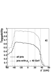
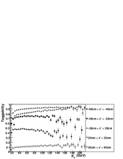
Figure 4: (a): taggability as a function of $z^{\prime}\equiv|z|\cdot\mbox{sign}(\eta\cdot z)$. The vertical lines denote the boundaries chosen for the parametrization in $p_{T}$ and $|\eta|$. (b): taggability as a function of jet $p_{T}$, in different bins of $z^{\prime}$. The curves for the two central bins are very similar and have been combined.

The tagging algorithms discussed in subsequent chapters are applied only to jets retained by the taggability criterion, and also the quoted performances do not account for the inefficiency incurred by this criterion.

3.3 $V^{0}$ rejection

By construction, the lifetime tagging algorithms assume that any measurable lifetime is indicative of heavy flavor jets. However, light strange hadrons also decay weakly, with long lifetimes. Particularly pernicious backgrounds arise from $K_{S}$ and $\Lambda$, as their lifetimes (90 ps and 263 ps, respectively) do not differ vastly from those of $b$ hadrons. In addition, $\gamma\rightarrow e^{+}e^{-}$ conversions may occur in the detector material at large distances from the beam line.

$K_{S}$ and $\Lambda$ candidates, commonly denoted as $V^{0}$s, are identified through two oppositely charged tracks satisfying the following criteria:

• The significance of the distance of closest approach (DCA) to the selected primary vertex in the transverse plane, $\mathcal{S}_{d}$ (see Sec. 2.1), of both tracks must satisfy $|\mathcal{S}_{d}|>3$.

• The tracks’ $z$ coordinates at the point of closest approach in the transverse plane must be displaced from the primary vertex less than 1 cm, to suppress misreconstructed tracks.

• The resulting $V^{0}$ candidate must have a distance of closest approach to the primary vertex of less than 200 $\mu$m. This requirement is intended to select only those $V^{0}$ candidates originating from the primary vertex, while candidates originating from heavy flavor decays may be taken into account during the tagging.

• The reconstructed mass should satisfy $472\mbox{ MeV}<m<516\mbox{ MeV}$ for $K_{S}$ candidates, and $1108\mbox{ MeV}<m<1122\mbox{ MeV}$ for $\Lambda$ candidates (in the latter case, the higher $p_{T}$ tracks are considered to be protons; the other tracks, or both tracks in the case of $K_{S}$ reconstruction, are assumed to be charged pions). The invariant mass distributions of reconstructed $K_{S}$ and $\Lambda$ candidates are shown in Fig. 5.

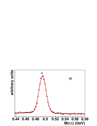
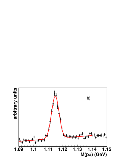
Figure 5: Reconstructed $K_{S}$ (a) and $\Lambda$ (b) mass peaks.

The $V^{0}$ finding efficiency depends on the transverse momentum of the $V^{0}$ decay products, as well as on the position of the decay vertex inside the tracker volume. As an example, Fig. 6 shows the $K_{S}$ finding efficiency as a function of the transverse position of the decay vertex for the cases when both or at least one of the decay pions have a transverse momentum greater than 1 GeV. This efficiency has been determined using simulated multijet events.

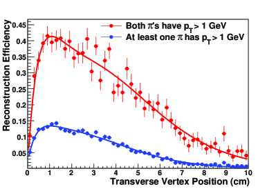
Figure 6: The $K_{S}\rightarrow\pi^{+}\pi^{-}$ finding efficiency as a function of the transverse position of the decay vertex as determined in simulated multijet events.

Photon conversions are most easily recognized by the fact that the opening angle between the electron and positron is negligibly small. In the plane perpendicular to the beam line, this is exploited by requiring that the tracks be less than 30 $\mu$m apart at the location where their trajectories are parallel to each other. In addition, they must again be oppositely charged, and their invariant mass is required to be less than 25 MeV. Since conversions happen inside material, the locations of their vertices reflect the distribution of material inside the detector, as illustrated by Fig. 7: the locations of the SMT barrel ladders and the disks are clearly visible in the distribution of the radial and $z$ coordinates, respectively, of reconstructed photon conversions.

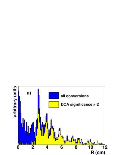
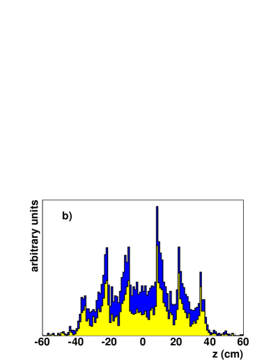
Figure 7: Reconstructed radial (a) and $z$ coordinate (b) of candidate conversion vertices. The peaks correspond to the radial positions of the SMT barrels and $z$ positions of the SMT disk structures, respectively.

4 The Secondary Vertex Tagger

The vast majority of $b$-hadron decays give rise to multiple charged particles emanating from the $b$-hadron’s decay point. The most intuitive tagging method is therefore to attempt to reconstruct this decay point explicitly and to require the presence of a displaced or secondary vertex. The requirement that a number of tracks all be extrapolated to the same point in three dimensions is expected to lead to an algorithm, the Secondary Vertex Tagger (SVT) [13], which is robust even in the presence of misreconstructed tracks.

After the identification and selection of the primary interaction vertex, the reconstruction of secondary vertices starts from the track jet associated with each (taggable) calorimeter jet (see Sec. 3.2). The tracks considered are those associated with the track jet, subject to additional selection criteria: they should have at least two SMT hits, transverse momentum exceeding $0.5\mbox{ GeV}$, transverse impact parameter with respect to the primary vertex $|d|<$ 1.5 mm, and a separation in the $z$ direction between the point of closest approach to the beam line and the primary vertex less than 4 mm. Subsequently, tracks associated with identified $V^{0}$ vertices (see Sec. 3.3) are removed from consideration. All remaining tracks are used in a so-called build-up vertex finding algorithm. In detail, the algorithm consists of the following steps:

1. Tracks within track jets with large transverse impact parameter significance, $|\mathcal{S}_{d}|>3$, are selected.

2. Vertices are reconstructed from all pairs of tracks using a Kalman vertex fitting technique [14], and are retained if the vertex fit yields a goodness-of-fit $\chi^{2}<\chi^{2}_{\max}=100$.

3. Additional tracks pointing to these seed vertices are added one by one, according to the resulting $\chi^{2}$ contribution to the vertex fit. The combination yielding the smallest increase in fit $\chi^{2}$ is retained.

4. This procedure is repeated until the increase in fit $\chi^{2}$ exceeds a set maximum, $\Delta\chi^{2}_{\max}=15$, or the total fit $\chi^{2}$ exceeds $\chi^{2}_{\max}$.

5. The resulting vertex is selected if in addition, the angle $\zeta$ between the reconstructed momentum of the displaced vertex (computed as the sum of the constituent tracks’ momenta) and the direction from the primary to the displaced vertex (in the transverse plane) satisfies $\cos\zeta>0.9$, and the vertex decay length in the transverse direction $L_{xy}<2.6$ cm.

6. Many displaced vertex candidates may result, with individual tracks possibly contributing to multiple candidates. Duplicate displaced vertex candidates are removed until no two candidates are associated with identical sets of tracks.

7. Secondary vertices are associated with the nearest calorimeter jets if $\Delta\mathcal{R}(\mbox{vertex},\mbox{jet})<0.5$. Here, the vertex direction is computed as the difference of the secondary and primary vertex positions.

Figure 8 shows distributions that characterize the properties of $b$-jet and light-flavor secondary vertices reconstructed in $t\bar{t}$ events simulated using the Alpgen [15] event generator: the multiplicity of vertices found in a track jet ($N_{\mbox{\scriptsize vtx}}$), the number of tracks associated with the vertex ($N_{\mbox{\scriptsize trk}}$), the mass of the vertex ($m_{\mbox{\scriptsize vtx}}$) calculated as the invariant mass of all track four-momentum vectors assuming that all particles are pions, and the largest decay length significance, $\mathcal{S}_{xy}\equiv L_{xy}/\sigma(L_{xy})$, where $\sigma(L_{xy})$ represents the uncertainty on $L_{xy}$.

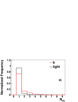
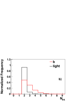
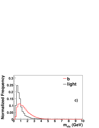
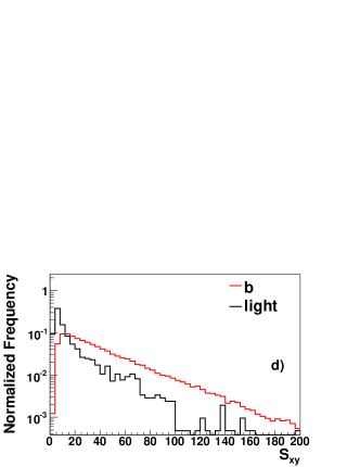
Figure 8: Properties of the secondary vertices for tagged $b$ and light jets in $t\bar{t}$ MC: multiplicity of vertices found in a track jet (a), the number of tracks associated with the vertex (b), the mass of the vertex (c), and the decay length significance (d).

A calorimeter jet is tagged as a $b$ jet if it has at least one secondary vertex with decay length significance greater than a nominal value. In order to characterize the performance of this tagging algorithm, various versions have been studied, differing in the requirements used in the selection procedure.

The algorithm as described above is referred to as the Loose algorithm. In Sec. 7.1.1 a high-efficiency version, labeled SuperLoose, with a correspondingly high tagging rate for light-flavor jets is also used. The high efficiency is obtained by placing no requirement on the impact parameter significance of the tracks used to reconstruct the secondary vertices.

5 The Jet Lifetime Probability Tagger

The impact parameters of all tracks associated with a calorimeter jet can be combined into a single variable, the Jet Lifetime Probability (JLIP) $\mathcal{P}_{\mbox{\scriptsize JLIP}}$ [16, 17, 18], which can be interpreted as the confidence level that all tracks in a jet originate from the (selected) primary interaction point. Jets from light quark fragmentation are expected to present a uniform $\mathcal{P}_{\mbox{\scriptsize JLIP}}$ distribution between 0 and 1, whereas jets from $c$ and $b$ quarks will exhibit a peak at a very low $\mathcal{P}_{\mbox{\scriptsize JLIP}}$ value. It is thus easy to select $b$-quark jets by requiring this probability not to exceed a given threshold, the value of which depends on the signal efficiency and background rejection desired for a given physics analysis.

Using the impact parameters of reconstructed tracks allows control of their resolution by using data, minimizing the need for simulated samples. For this purpose, the impact parameter is signed by using the coordinates of the track at the point of closest approach to the fitted primary vertex, ${\vec{d}}$, and the jet momentum vector, ${\vec{}p_{T}}$(jet). In the plane transverse to the beam axis, the distance of closest approach to the primary vertex ($d=|{\vec{d}}|$) is given the same sign as the scalar product ${\vec{d}}\cdot{\vec{}p_{T}}$(jet). The signed $d$ distribution for tracks from light quark fragmentation is almost symmetric, whereas the distribution for tracks from $b$-hadron decay exhibits a long tail at positive values. Therefore, provided that the sign of ${\vec{d}}\cdot{\vec{}p_{T}}$(jet) is correctly determined, the negative part of the $d$ distribution allows the $d$ resolution function to be parametrized.

5.1 Calibration of the impact parameter resolution

In order to tune the impact parameter uncertainty, $\sigma_{d}$, computed from the track fit, the following variable is introduced: $p_{\mbox{\scriptsize scat}}=p(\sin\theta)^{3/2}$, where $p$ is the particle momentum and $\theta$ its polar angle relative to the beam axis. In the plane transverse to the beam axis, the smearing due to multiple scattering is inversely proportional to $p_{T}=p\sin\theta$ and proportional to the square root of the distance traveled by the track. Assuming the detector material to be distributed along cylinders aligned with the beam, this distance is also inversely proportional to $\sin\theta$. The $d$ distributions are then computed in sixteen different $p_{\mbox{\scriptsize scat}}$ intervals.

In order to parametrize the $d$ resolution, five track categories are considered:

• at most six CFT hits (each doublet layer may give rise to one hit) and at least one SMT hit in the innermost layer, for tracks with $|\eta|>1.6$;

• at least seven CFT hits and 1, 2, 3, or 4 SMT superlayer hits (the eight SMT barrel layers are grouped into four superlayers; the two neighboring layers constituting one superlayer provide full azimuthal acceptance).

The first category includes forward tracks outside the full CFT acceptance, the latter are central tracks with different numbers of SMT hits.

The calibration is performed starting from the impact parameter significance $\mathcal{S}_{d}=d/\sigma_{d}$, with the sign of $d$ determined as described above. In each $p_{\mbox{\scriptsize scat}}$ interval and for each category, the $\mathcal{S}_{d}$ distribution is fitted using a Gaussian function to describe the $d$ resolution. The fitted pull values (the variance of the Gaussian) are presented in Fig. 9 for multijet data. The same calibration procedure is carried out for simulated QCD events, and the corresponding results are also shown in Fig.  9. The superimposed curves are empirical parametrizations of the data and the simulation. The pull values are found to go up to 1.2 in data, while they are closer to 1 in the simulation.

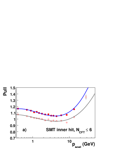
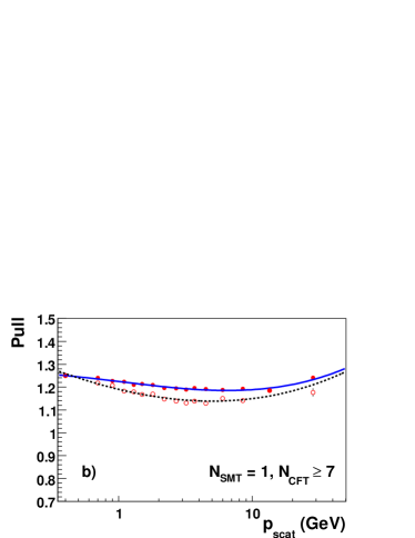
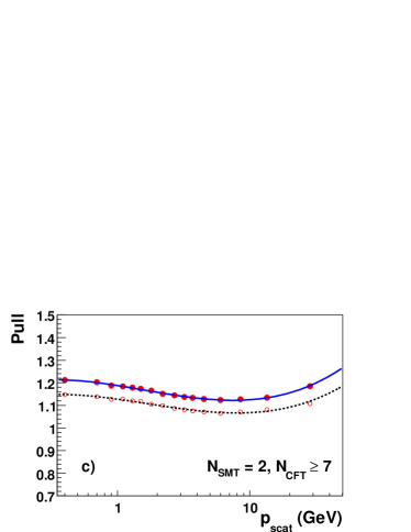
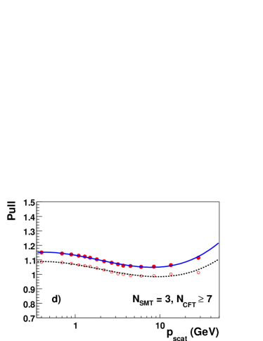
Figure 9: Fitted pull values of the track impact parameters as a function of $p_{\mbox{\scriptsize scat}}=p(\sin\theta)^{3/2}$, for different track categories. The superimposed solid (dashed) curves are empirical parametrizations of the data (QCD MC).

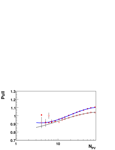
Figure 10: Fitted pull values of the track impact parameters, corrected here for their $p_{\mbox{\scriptsize scat}}$ and category dependence, as a function of the number of tracks attached to the primary vertex, combining all track categories. The superimposed solid (dashed) curves are empirical parametrizations of the data (QCD MC).

As the impact parameter resolution may be sensitive to the primary vertex resolution, the $d$ significance is also fitted separately for events with different numbers of tracks, $N_{\mbox{\scriptsize PV}}$, attached to the primary vertex. As shown in Fig. 10 for multijet data and simulated QCD events, the pull value increases significantly with $N_{\mbox{\scriptsize PV}}$ (here the $p_{\mbox{\scriptsize scat}}$ and category dependence of the pull value is already corrected for).

Then for each track, the impact parameter uncertainty and associated significance are corrected according to the track’s measured $p_{\mbox{\scriptsize scat}}$ value, category $i$ and number of tracks $N_{\mbox{\scriptsize PV}}$ attached to the primary vertex:

$$\sigma_{d}^{\mbox{\scriptsize corr}} = \mbox{pull}(p_{\mbox{\scriptsize scat}},i,N_{\mbox{\scriptsize PV}})\cdot\sigma_{d}$$ (4)

$$\mathcal{S}_{d}^{\mbox{\scriptsize corr}} = \mathcal{S}/\mbox{pull}(p_{\mbox{\scriptsize scat}},i,N_{\mbox{\scriptsize PV}})\;$$

The corrected $\sigma_{d}^{\mbox{\scriptsize corr}}$ resolutions are shown in Fig. 11 for multijet data and simulated QCD events. In the approximation of small angles [1], they can be parametrized as

$$\sigma^{\mbox{\scriptsize corr}}_{d}=\frac{a}{p\;(\sin\theta)^{3/2}}\oplus b,$$ (5)

where $a$ describes multiple scattering effects, and $b$ is the asymptotic resolution (which is sensitive to the primary vertex resolution, detector alignment, SMT intrinsic resolution, etc.); the symbol $\oplus$ denotes their summing in quadrature. This parametrization is superimposed in Fig. 11.

The impact parameter resolution is observed to be better in the simulation than in data. For forward tracks with fewer than 7 CFT hits and with $p_{\mbox{\scriptsize scat}}>10\mbox{ GeV}$, the multiple-scattering small angles approximation is no longer valid. This can lead to misreconstructed track momenta, and consequently the measured $d$ resolution is larger than its asymptotic fitted value (see Fig. 11a). The parametrization is also imperfect at the lowest $p_{\mbox{\scriptsize scat}}$ values, although the reason for this has not been ascertained.

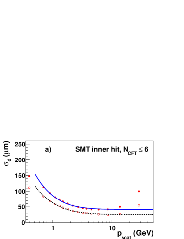
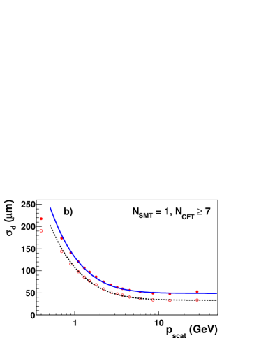
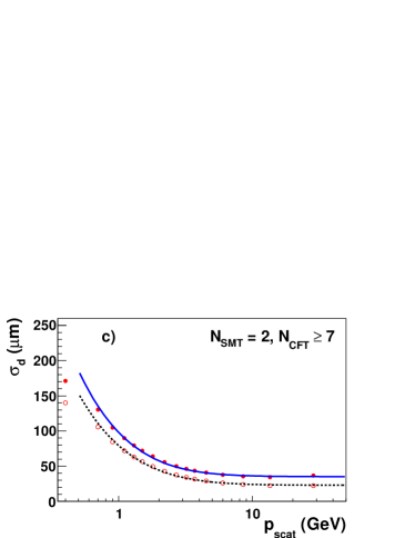
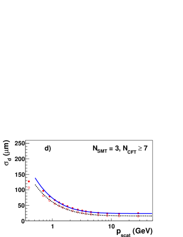
Figure 11: Corrected track impact parameter resolution as a function of $p_{\mbox{\scriptsize scat}}$, for different track categories. The solid (dashed) curve is a fit to the data (QCD MC).

5.2 Lifetime probability

The data are used to calibrate the impact parameter significance. For multijet data or QCD MC, the negative part of the $d$ significance distribution, denoted impact parameter resolution function $\mathcal{R}(\mathcal{S}_{d}^{\mbox{\scriptsize corr}})$, is parametrized as the sum of four Gaussian functions, as illustrated in Fig. 12. After removing tracks originating from $V^{0}$ candidates (see Sec. 3), the track categories used in the previous section are extended to take into account the number of SMT and CFT hits, $|\eta|$, fit $\chi^{2}$, and $p_{T}$ values of the tracks, as listed in Table 1. The category ranges are adjusted to describe as much as possible geometric and tracking effects. This further refinement results in 29 track categories.

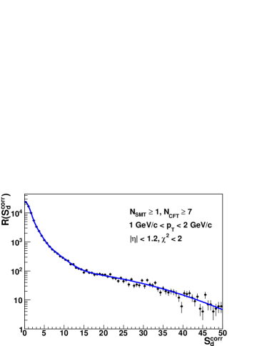
Figure 12: The impact parameter resolution functions, shown here for one of the 29 track categories described in Table 1, are parametrized as a sum of four Gaussian functions.

SMT hits	CFT hits	$|\eta|$	fit $\chi^{2}$	$p_{T}$ ( GeV)
$\geq 1$ inner layer hit	$\leq 6$	1.6–2, $>2$	$>0$	$>1$
1 superlayer	$\geq 7$	$<1.2$	0–2, $>2$	$>1$
”	”	$>1.2$	$>0$	$>1$
2, 3, 4 superlayers	$\geq 7$	$<1.2$	0–2	1–2, 2–4, $>4$
”	”	”	2–4, $>4$	$>1$
”	”	1.2–1.6	0–2, $>2$	$>1$
”	”	$>1.6$	$>0$	$>1$

Table 1: Track categories used for the parametrization of the impact parameter resolution functions. The “$\geq 1$ inner layer hit” line denotes the requirement of at least one hit in the innermost SMT superlayer.

For tracks with positive $d$, the parametrized resolution function is then converted into a probability for this track to originate from the primary interaction point

$$\mathcal{P}_{\mbox{\scriptsize trk}}(\mathcal{S}_{d}^{\mbox{\scriptsize corr}})=\frac{\int_{-\infty}^{-|\mathcal{S}_{d}^{\mbox{\scriptsize corr}}|}\mathcal{R}(s)ds}{\int_{-\infty}^{0}\mathcal{R}(s)ds}\;.$$ (6)

The corresponding track probabilities are shown in Fig. 13 for multijet data and simulated jets of different flavors, and for positive and negative $d$ values. Tracks with negative $d$ values in multijet data and in simulated light quark jets are used to define the $d$ resolution functions, thus ensuring uniform $\mathcal{P}_{\mbox{\scriptsize trk}}(\mathcal{S}_{d}^{\mbox{\scriptsize corr}}<0)$ probability distributions. For positive $d$, a significant peak at low $\mathcal{P}_{\mbox{\scriptsize trk}}(\mathcal{S}_{d}^{\mbox{\scriptsize corr}}>0)$ probability is present in simulated $c$ and $b$ jets. In multijet data, a peak is also observed at low values which is partly due to the presence of $V^{0}$s (which are not all removed, see Sec. 3.3), but also to tracks from charm and $b$-hadron decays. Note that for simulated $c$ and $b$ jets, a slight peak remains at negative $d$ due to a flip of the $d$ sign, mainly due to tracks very close to the jet axis direction (see also Sec. 6). In addition, a small dip is observed at low $\mathcal{P}_{\mbox{\scriptsize trk}}(\mathcal{S}_{d}^{\mbox{\scriptsize corr}}<0)$. This dip is due to the fact that, like for the data, the resolution function for the simulated sample has been derived without removal of the heavy flavor component.

Finally, the selected $N_{\mbox{\scriptsize trk}}$ tracks with positive $d$ significance are used to compute the jet probability $\mathcal{P}_{\mbox{\scriptsize JLIP}}$ as

$$\mathcal{P}_{\mbox{\scriptsize JLIP}}\equiv\mathcal{P}^{+}_{\mbox{\scriptsize JLIP}} = \Pi\times\sum_{j=0}^{N_{\mbox{\scriptsize trk}}-1}\frac{(-\ln\Pi)^{j}}{j!}$$ (7)

$$\mbox{with}\;\;\;\Pi = \prod_{i=1}^{N_{\mbox{\scriptsize trk}}}\mathcal{P}_{\mbox{\scriptsize trk}}(\mathcal{S}^{\mbox{\scriptsize corr}}_{d,i})\;.$$

For tracks with negative $d$, a jet probability $\mathcal{P}^{-}_{\mbox{\scriptsize JLIP}}$ can be computed analogously.

By construction, if the $\mathcal{P}_{\mbox{\scriptsize trk}}$ are uniformly distributed and uncorrelated, $\mathcal{P}_{\mbox{\scriptsize JLIP}}$ will also be uniformly distributed, independent of $N_{\mbox{\scriptsize trk}}$ [19]. Therefore, apart from wrongly assigned negative $d$ in the case of tracks originating from the decay of long-lived particles, and from any correlations that are induced by the common primary vertex (which is reconstructed from the tracks under consideration, among others), the resulting $\mathcal{P}_{\mbox{\scriptsize JLIP}}$ distribution is indeed expected to be uniform for negative $d$ tracks in multijet data. These distributions are shown in Fig. 14 for multijet data and simulated jets of different flavors, and for positive and negative $d$ values. Applying this tagging algorithm simply entails requiring that a jet’s $\mathcal{P}_{\mbox{\scriptsize JLIP}}$ value does not exceed some given maximum value.

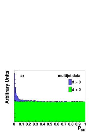
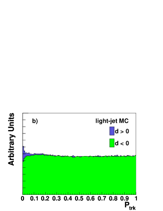
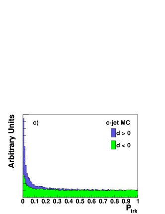
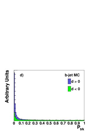
Figure 13: Track probability ($\mathcal{P}_{\mbox{\scriptsize trk}}$, see Eq. 6) distribution in multijet data (a) and QCD MC simulation of light-flavor (b), $c$ (c), and $b$ (d) jets, for positive (dark histograms) and negative (light histograms) $d$ values.

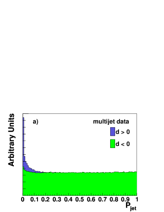
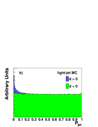
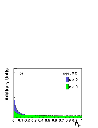
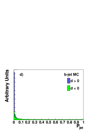
Figure 14: Jet probability ($\mathcal{P}_{\mbox{\scriptsize JLIP}}$) distribution in multijet data (a) and QCD MC simulation of light-flavor (b), $c$ (c), and $b$ (d) jets, for positive (dark histograms) and negative (light histograms) $d$ values.

6 The Counting Signed Impact Parameter Tagger

In this method [20], as in Sec. 5, there is no attempt to use reconstructed secondary vertices. Instead, the signed impact parameter significance $S_{d}$ is calculated for all good tracks located within a $\mathcal{R}=0.5$ cone around the jet axis. For the present purpose, the definition of a good track is as follows:

• the track should be associated with the hard interaction (the difference between the $z$ coordinates of the DCA point and the primary vertex should be less than 1 cm);

• the track DCA must not be too large, $|d|<2$ mm;

• the track transverse momentum should satisfy $p_{T}>1\mbox{ GeV}$;

• the track fit should be of good quality: its $\chi^{2}$ per degree of freedom $\chi^{2}_{\mbox{\scriptsize dof}}$ should satisfy $\chi^{2}_{\mbox{\scriptsize dof}}<9$;

• tracks with $\chi^{2}_{\mbox{\scriptsize dof}}<3$ are required to have at least 2 SMT hits;

• tracks with $3\leq\chi^{2}_{\mbox{\scriptsize dof}}<9$ are required to have either 4 SMT hits and at least 13 CFT hits, or at least 5 SMT hits and either 0 or at least 11 CFT hits.

The effect of the last criterion is to impose more stringent quality requirements on tracks having $|\eta|\approx 1.5$. This is done as this region suffers from a higher fake track rate, leading to track candidates with a small but non-zero number of CFT hits. Finally, tracks originating from a $V^{0}$ candidate, as detailed in Sec. 3, are also excluded.

A jet is considered to be tagged by the Counting Signed Impact Parameter (CSIP) tagger if there are at least two good tracks with $\mathcal{S}_{d}/a>3$ or at least three good tracks with $\mathcal{S}_{d}/a>2$, where $a$ is a scaling parameter. The choice of $a$ determines the operating point ($b$-tagging efficiency and mistag rate) of the algorithm. Alternatively, if a jet has at least two good tracks with positive $\mathcal{S}_{d}$, then the minimum value of $a$ at which there are at least two good tracks with $\mathcal{S}_{d}/a>3$ or at least three good tracks with $\mathcal{S}_{d}/a>2$ can be used as a continuous output variable of the tagger. Here, $a$ is set to 1.2, as suggested by optimization studies using simulated data.

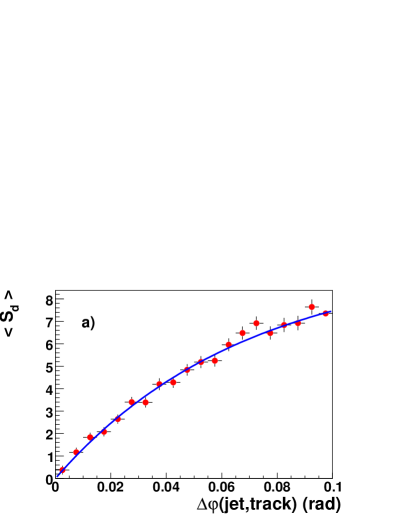
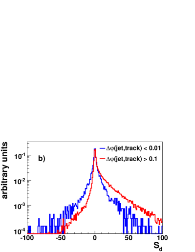
Figure 15: Mean signed impact parameter significance $\mathcal{S}_{d}$ (averaged over all tracks in all $b$-jets in simulated events) as a function of the azimuthal angle between the track and $b$-jet directions $\Delta\varphi$ (a) and $\mathcal{S}_{d}$ distributions for tracks at low and high $\Delta\varphi$ (b).

In the actual implementation of the algorithm, there is an additional condition related to the fact that the sign of $\mathcal{S}_{d}$ cannot be determined accurately for tracks that are very close to the jet axis, as illustrated by Fig. 15. The criterion of closeness is empirically chosen as the difference in the azimuthal angle between the track and jet directions, $\Delta\varphi$, being less than $\Delta\varphi_{0}=$ 20 mrad. This value has been optimized by comparing algorithm performance for various values of $\Delta\varphi_{0}$. Four categories of tracks are counted separately:

• tracks with $\mathcal{S}_{d}/a>3$, $|\Delta\varphi|>\Delta\varphi_{0}$ (“$3\sigma$-strong” tracks, their total number to be denoted as $N_{3s}$),

• tracks with $2<\mathcal{S}_{d}/a<3$, $|\Delta\varphi|>\Delta\varphi_{0}$ (“$2\sigma$-strong” tracks, $N_{2s}$),

• tracks with $|\mathcal{S}_{d}/a|>3$, $|\Delta\varphi|<\Delta\varphi_{0}$ (“$3\sigma$-weak” tracks, $N_{3w}$),

• tracks with $2<|\mathcal{S}_{d}/a|<3$, $|\Delta\varphi|<\Delta\varphi_{0}$ (“$2\sigma$-weak” tracks, $N_{2w}$).

If CSIP is used as a stand-alone algorithm, the jet is considered tagged if $N_{2s}+N_{3s}+N_{2w}+N_{3w}\geq 3$ and $N_{2s}+N_{3s}\geq 1$, or $N_{3s}+N_{3w}\geq 2$ and $N_{3s}\geq 1$. In other words, in addition to the original tagging condition (at least two good tracks with $\mathcal{S}_{d}/a>3$ or at least three good tracks with $\mathcal{S}_{d}/a>2$), at least one of the tagging tracks is required to be strong. In the present implementation, the four numbers ($N_{3s}$, $N_{2s}$, $N_{3w}$, $N_{2w}$) are packed in a single variable which is used in the combined algorithm, as explained in Sec. 7.

7 The Neural Network Tagger

Artificial neural networks (see e.g. [21]) are modeled after the synaptic processes in the brain, and have proved to be a versatile machine learning approach to the general problem of separating samples of events characterized by many event variables. In particular, the potential of neural networks to exploit the correlations between variables, and the possibility to train the network to recognize such correlations, make their use in high energy physics attractive.

The neural network (NN) tagger attempts to discriminate between $b$ jets and other jet flavors by combining input variables from the SVT, JLIP, and CSIP tagging algorithms [22]. The NN implementation chosen is the TMultiLayerPerceptron from the root [23] framework.

7.1 Optimization

The following NN parameters were optimized: input variables (number and type), NN structure, number of training epochs, and jet selection criteria. The choice of input variables is crucial for the performance of the NN and so was optimized first.

The NN parameters were optimized by minimizing the light-flavor tagging efficiency or fake rate for fixed benchmark $b$-tagging efficiencies. The optimization plots were produced from a high $p_{T}$ Alpgen $t\bar{t}$ sample and cross checked with a Pythia [24] $b\bar{b}$ sample to ensure there was no sample, $p_{T}$, or MC generator dependence in the optimization.

The NN was trained on simulated multijet light-flavor and $b\bar{b}$ samples. To avoid overtraining, i.e., a focus on features that are too event specific, the signal sample of 270 000 $b\bar{b}$ events and the background sample of 470 000 light-flavor events were each split in half, with one half used as the training sample and the other half to evaluate the network’s performance. It was verified that for the parameter settings as described below, no overtraining occurs.

7.1.1 Input variables

Initially, a large number of lifetime-related variables were investigated (e.g. variables for different SVT versions, or various combinations of the numbers of tracks in the different CSIP track categories). After a first assessment of their performance, nine input variables were selected for the final input variable optimization due to their good discrimination between $b$ jets and light-flavor jets. Six of the variables are based on the secondary vertices reconstructed using the SVT algorithm. The remaining three summarize information from the JLIP and CSIP algorithms. The input variables are:

SVT $\mathcal{S}_{xy}$:

the decay length significance (the decay length in the transverse plane divided by its uncertainty) of the secondary vertex with respect to the primary vertex.

SVT $\chi^{2}_{\mbox{\scriptsize dof}}$:

the $\chi^{2}$ per degree of freedom of the secondary vertex fit.

SVT $N_{\mbox{\scriptsize trk}}$:

the number of tracks used to reconstruct the secondary vertex.

SVT $m_{\mbox{\scriptsize vtx}}$:

the mass of the secondary vertex.

SVT $N_{\mbox{\scriptsize vtx}}$:

the number of secondary vertices reconstructed in the jet.

SVT $\Delta\mathcal{R}$:

the distance in ($\eta$,$\phi$) space between the jet axis and the difference between the secondary and primary vertex positions.

JLIP $\mathcal{P}_{\mbox{\scriptsize JLIP}}$:

the “jet lifetime probability” computed in Sec. 5.

JLIP $\mathcal{P}_{\mbox{\scriptsize RedJLIP}}$:

JLIP $\mathcal{P}_{\mbox{\scriptsize JLIP}}$ re-calculated with the track with the highest significance removed from the calculation.

CSIP $\mathcal{N}_{\mbox{\scriptsize CSIP}}$:

a combined variable based on the number of tracks with an impact parameter significance greater than an optimized value. This variable is discussed in more detail below.

Since more than one secondary vertex can be found for each jet, vertex variables are ranked in order of the most powerful discriminator, the decay length significance ($\mathcal{S}_{xy}$). The secondary vertex with the largest $\mathcal{S}_{xy}$ in a jet is used to provide the input variables. If no secondary vertex is found, the SVT values are set to 0, apart from the SVT $\chi^{2}_{\mbox{\scriptsize dof}}$ which is set to 75 corresponding to the upper bound of $\chi^{2}_{\mbox{\scriptsize dof}}$ values.

The standard, Loose, implementation of the SVT algorithm requires a displaced vertex constructed from significantly displaced tracks. While such an approach helps to isolate a pure sample of heavy flavor decays, it typically results in a low efficiency. In the context of an NN optimization, this is undesirable as any vertex-related information is only available if a displaced vertex is found. For this reason, the SuperLoose SVT algorithm described in Sec. 4 is used: even if the vertex candidates it finds are a less pure sample, it finds significantly more displaced vertices and they provide additional discrimination between $b$ jets and other flavors. Figure 16 shows the efficiency, as a function of jet $p_{T}$, for both algorithm choices for light-flavor and $b$ jets. The NN tagger is found to perform best if information from both the SuperLoose and the Loose SVT algorithms is used: the $N_{\mbox{\scriptsize trk}}$ variable is taken from the latter, and all other SVT variables from the former.

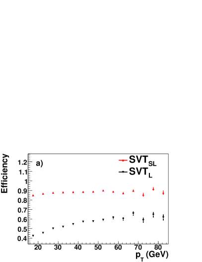
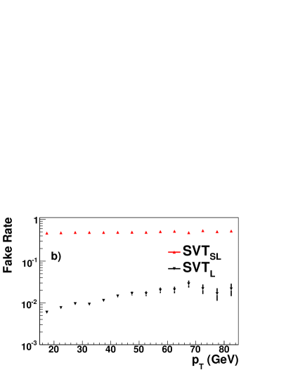
Figure 16: Efficiencies of the SuperLoose (SVT_SL, up triangles) and Loose (SVT_L, down triangles) SVT taggers for $b\bar{b}$ (a) and light-flavor (b) MC jets.

The CSIP $\mathcal{N}_{\mbox{\scriptsize CSIP}}$ variable is based on the four CSIP variables $N_{3s}$, $N_{2s}$, $N_{3w}$, and $N_{2w}$ described in Sec. 6. Neural networks tend to perform best when provided with continuous values. Since the CSIP variables have small integer values which are not very good as inputs, they are combined in one variable which brings the advantage of reducing the number of input variables, hence simplifying the NN:

$$\mathcal{N}_{\mbox{\scriptsize CSIP}}=6\times N_{3s}+4\times N_{2s}+3\times N_{3w}+2\times N_{2w}.$$ (8)

The weights were determined in an empirical manner to give optimum performance for this variable alone.

First, the input variables were optimized. At this stage, the other NN parameters were set to the following values: NN structure $N$:2$N$:1, where $N$ is the number of input variables; 500 training epochs; and selection criteria SVT_SL $\mathcal{S}_{xy}>2$ or CSIP $\mathcal{N}_{\mbox{\scriptsize CSIP}}>8$ or JLIP $\mathcal{P}_{\mbox{\scriptsize JLIP}}<0.02$. (The subscript $SL$ serves to clarify that this variable is obtained from the SuperLoose SVT algorithm, as described above.)

The input variables were optimized by first identifying the two most powerful input variables by testing every possible combination in a two-input NN, resulting in the choice of $\mathcal{S}_{xy}$ and $\mathcal{N}_{\mbox{\scriptsize CSIP}}$ as initial variables. Starting with an initial NN with these $n=2$ variables and a list of $m$ variables, the remaining variables were then ranked in order of power using the following procedure:

1. each of the $m$ variables to be tested was added individually to the initial $n$ variable NN, resulting in $m$ NNs with $n+1$ variables each;

2. the variable whose addition yielded the largest improvement in NN performance was identified. This variable was added permanently to the $n$ variable NN;

3. the above steps were repeated, testing each of the remaining $m-1$ variables with the new $n+1$ variable NN.

The fake rate of each NN at a 70% $b$-jet efficiency benchmark scenario was used to select the optimal variable. As a cross check, the procedure was repeated for signal efficiencies ranging from 50% to 75% in 5% steps. The same set of variables was found to give the greatest reduction in fake rate in each case. As an example, two benchmark scenarios are shown in Fig. 17.

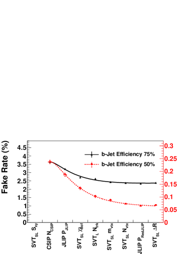
Figure 17: Fake rate for fixed signal efficiencies of $75\%$ (up triangles, left axis) and $50\%$ (down triangles, right axis) as a function of additional NN variables. The NN variables were added to the NN in order of performance. The lines are intended to guide the eye only. The errors are statistical only.

The NNs with seven to nine variables have the best performance. Therefore the seven variable NN is chosen as the optimal solution, keeping the NN as simple as reasonably possible. The final selected variables, ranked in order of performance, are SVT_SL $S_{xy}$, CSIP $\mathcal{N}_{\mbox{\scriptsize CSIP}}$, JLIP $\mathcal{P}_{\mbox{\scriptsize JLIP}}$, SVT_SL $\chi^{2}_{\mbox{\scriptsize dof}}$, SVT_L $N_{\mbox{\scriptsize trk}}$, SVT_SL $m_{\mbox{\scriptsize vtx}}$, and SVT_SL $N_{\mbox{\scriptsize vtx}}$. The distributions of these variables in simulated QCD samples are shown in Fig. 18.

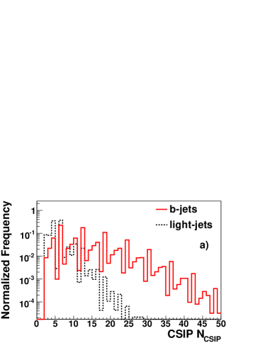
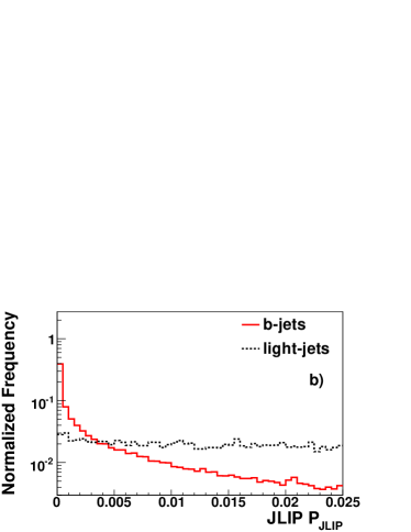
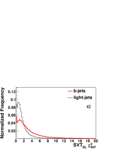
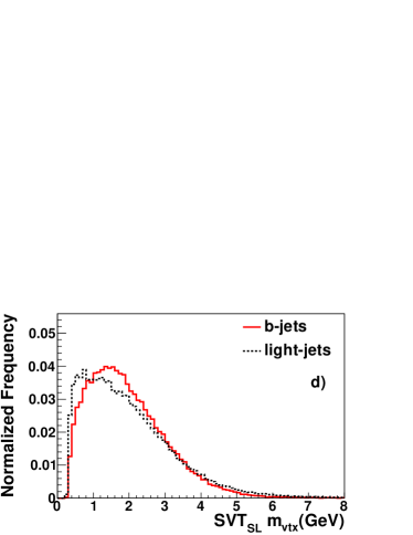
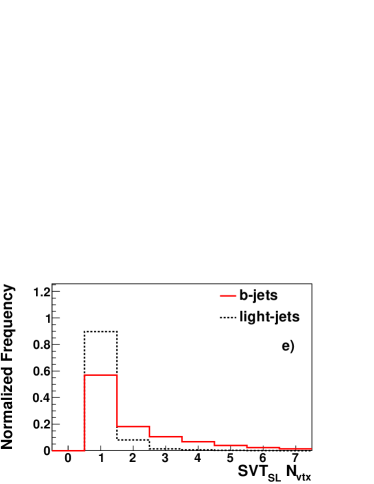
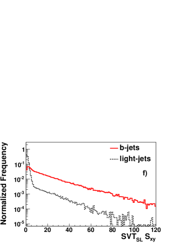
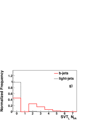
Figure 18: The NN variables CSIP $\mathcal{N}_{\mbox{\scriptsize CSIP}}$ (a), JLIP $\mathcal{P}_{\mbox{\scriptsize JLIP}}$ (b), SVT_SL $\chi^{2}_{\mbox{\scriptsize dof}}$ (c), $m_{\mbox{\scriptsize vtx}}$ (d), $N_{\mbox{\scriptsize vtx}}$ (e), $S_{xy}$ (f), and SVT_L $N_{\mbox{\scriptsize trk}}$ (g) for QCD $b\bar{b}$ MC (continuous lines), and light jet QCD MC (dashed lines). All histograms are normalized to unit area.

7.1.2 Number of training epochs and neural network structure

The number of training epochs was varied from 50 up to 2000. For each of the benchmark scenarios the majority of the minimization is reached by $\approx 400$ epochs, with only small further improvement thereafter.

The number of hidden layers was set to one, as one layer should be sufficient to model any continuous function [25] and this minimizes CPU usage. The number of hidden nodes was optimized by varying their number from seven through thirty-four. Twenty-four was chosen as the optimal number of hidden nodes.

7.1.3 Input selection criteria

Another important attribute of the NN is the selection of the jets which are used to train the NN. A selection too loose can cause a loss of performance as the NN training is dominated by signal and background jets which could have been separated with a simple requirement, causing a loss of resolution. A selection which is too tight will cause a significant loss of $b$ jets and therefore limit the maximum possible efficiency.

The input selection criteria were optimized by considering each variable in turn, starting with the most important variable, SVT_SL $\mathcal{S}_{xy}$, then JLIP $\mathcal{P}_{\mbox{\scriptsize JLIP}}$, and finally CSIP $\mathcal{N}_{\mbox{\scriptsize CSIP}}$ (at this stage, a requirement on JLIP $\mathcal{P}_{\mbox{\scriptsize JLIP}}$ performs better than one on CSIP $\mathcal{N}_{\mbox{\scriptsize CSIP}}$). The optimal values were chosen as SVT_SL $\mathcal{S}_{xy}>$ 2.5, JLIP $\mathcal{P}_{\mbox{\scriptsize JLIP}}<~{}0.02$, and CSIP $\mathcal{N}_{\mbox{\scriptsize CSIP}}>~{}8$. The results for SVT_SL $\mathcal{S}_{xy}$ are shown in Fig. 19 (in this case, the requirement is fixed at an $\mathcal{S}_{xy}$ value of 2.5 since for the loosest operating points, the performance degrades for even larger $\mathcal{S}_{xy}$ values).

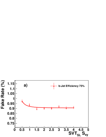
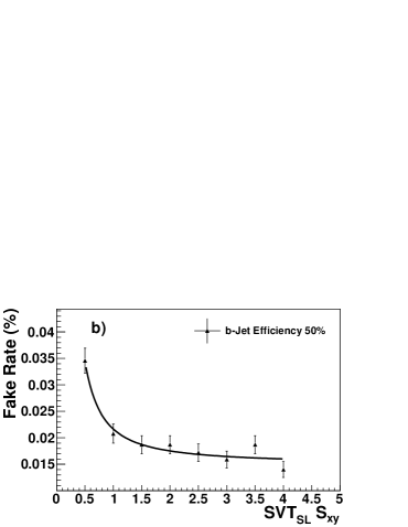
Figure 19: Fake rate for fixed signal efficiencies of $75\%$ (a) and $50\%$ (b) as a function of the SVT_SL $\mathcal{S}_{xy}$ requirement on the input jets. The lines are intended to guide the eye only.

7.1.4 Optimized NN parameters

The optimized parameter values for the NN tagger are summarized in Table 2.

Parameter	Value
NN structure	7 input nodes:24 hidden nodes:1 output node
Input variables	(1) SVTSL $\mathcal{S}_{xy}$ (2) CSIP $\mathcal{N}_{\mbox{\scriptsize CSIP}}$ (3) JLIP $\mathcal{P}_{\mbox{\scriptsize JLIP}}$ (4) SVTSL $\chi^{2}_{\mbox{\scriptsize dof}}$
(performance ranked)	(5) SVTL $N_{\mbox{\scriptsize trk}}$ (6) SVTSL $m_{\mbox{\scriptsize vtx}}$ (7) SVTSL $N_{\mbox{\scriptsize vtx}}$
Input selection criteria	SVTSL $\mathcal{S}_{xy}>$ 2.5 or JLIP $\mathcal{P}_{\mbox{\scriptsize JLIP}}<~{}0.02$ or CSIP $\mathcal{N}_{\mbox{\scriptsize CSIP}}>~{}8$
(failure results in NN output of 0)
Number of training epochs	400

Table 2: Optimized NN parameters.

7.2 Performance

The output from the optimized NN $b$ tagger on $b\bar{b}$ and light-flavor simulated jets is shown in Fig. 20. There is a significant separation between the signal and background samples. It should be noted that the light-flavor jets in the distribution have all passed the loose tagging input selection criteria listed in Table 2.

The advantage of combining the input variables from several taggers in an NN is shown in Fig. 21, which compares the NN $b$-tagging performance to the JLIP, SVT and CSIP taggers. There is a substantial improvement, with relative efficiency increases of $\approx$ 20 – 50% for a fake rate of $0.2\%$ and $\approx 15\%$ for a fake rate of $4\%$. The fake rate is reduced by a factor of between two or three for fixed signal efficiencies.

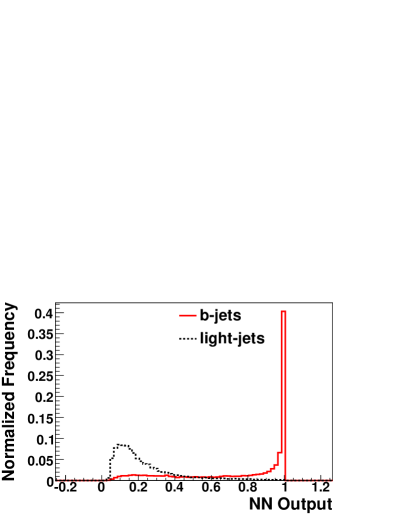
Figure 20: The NN output for light-flavor (dashed line) and $b$ (continuous line) jets (with $p_{T}>15\mbox{ GeV}$ and $|\eta|<2.5$) in simulated QCD events. Both distributions are normalized to unity.

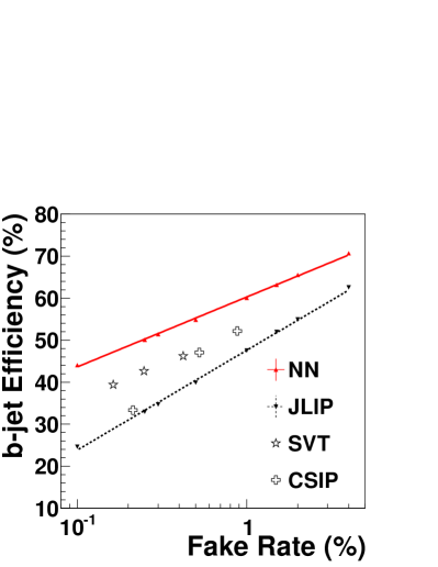
Figure 21: Performance of the NN (up triangles, continuous line), JLIP (down triangles, dotted line), CSIP (hollow crosses) and Loose SVT (hollow stars) taggers computed on simulated $Z\rightarrow b\bar{b}$ and $Z\rightarrow q\bar{q}$ jet samples. Due to the discrete nature of the CSIP and SVT taggers’ outputs a continuous performance curve is not shown.

The NN tagger performance in data is evaluated in the following sections for twelve operating points, corresponding to NN output discriminant threshold values ranging from 0.1 to 0.925. For illustrative purposes, detailed results will be provided for threshold values of 0.325 and 0.775, referred to as L2 and Tight, respectively.

8 Efficiency Estimation

The performance of the tagging algorithm cannot simply be inferred from simulated samples. Several effects cause differences between the data and these simulated samples:

• Simulated hit resolutions, both in the CFT and in the SMT, have been tuned to reproduce those in the data. However, the tuning cannot be expected to be perfect as the observed resolutions in the data are also affected by poorly understood geometrical effects which are not modeled in the simulation.

• A small but non-negligible fraction of the detector elements, in particular in the SMT, are disabled from time to time.

These effects lead to different effective resolutions and efficiencies in data and simulated samples. A calibration is therefore required. This section describes the estimation of the $b$- and $c$-jet tagging efficiencies, both of which are dominated by genuine heavy flavor decays. Jets originating from $u$, $d$, or $s$ quarks or from gluons are jointly referred to as light ($l$) jets. The light-jet tag rate estimation is described in Sec. 9.

8.1 MC and data samples

The data used in the performance measurements were collected from July 2002 to February 2006 and correspond to an integrated luminosity of $\approx 1~{}\mbox{fb}^{-1}$. The tagging efficiency in simulated events is measured using several processes simulated using the pythia ($Z\rightarrow b\bar{b}$, $Z\rightarrow c\bar{c}$, $Z\rightarrow q\bar{q}$, QCD) and alpgen (inclusive $t\bar{t}$) event generators. Large samples of simulated $b$ and $c$ jets are created by combining the appropriate flavor jets from the individual samples.

8.2 The SystemD method

The SystemD method [26] was developed to determine identification efficiencies using almost exclusively the data. Simulated samples are used only to estimate correction factors. The method involves several, essentially uncorrelated, identification criteria which are applied to the same data sample. Combining these criteria allows the definition of a system of equations which can be solved to extract the efficiency of each criterion.

The data sample is assumed to be composed of a signal and $n$ backgrounds. Denoting by $f_{0}$ the fraction of signal events, and by $f_{i=1\ldots n}$ the fraction of each considered background, these fractions must satisfy:

$$\sum_{i=0}^{n}f_{i}=1.$$ (9)

Subsequently, $m$ uncorrelated identification criteria are considered with different selection efficiencies $\varepsilon_{i=0\ldots n}^{k=1\ldots m}$ for the signal and backgrounds. Only a fraction $Q^{k}$ of the total number of events will pass the $k$-th identification criterion. Then a new set of equations can be added for each selection:

$$\sum_{i=0}^{n}\varepsilon_{i}^{k}f_{i}=Q^{k}.$$ (10)

If the selection criteria are uncorrelated, the total efficiency $\varepsilon_{i=0\ldots n}^{k_{1},\ldots,k_{r}}$ ($r\leq m$) of applying several of them successively can be factorized in terms of the individual efficiencies $\varepsilon_{i}^{k}$:

$$\varepsilon_{i}^{k_{1},\ldots,k_{r}}=\prod_{v=1}^{r}\varepsilon_{i}^{k_{v}}.$$ (11)

A generalization of Eq. (10) can then be obtained for a combination of several criteria:

$$Q^{k_{1},\ldots,k_{r}}=\sum_{i=0}^{n}\Big{(}\prod_{v=1}^{r}\varepsilon_{i}^{k_{v}}\Big{)}f_{i}.$$ (12)

The signal and background fractions are $n+1$ unknown parameters and each identification criterion introduces $n+1$ new unknowns in the form of selection efficiencies. The number of equations of the form of Eq. (12) depends on the number of combinations of the $m$ criteria, leading to a total of $\sum_{r=0}^{m}{r\choose m}=2^{m}$ equations. To obtain a system of equations which can be solved, $n$ and $m$ must satisfy

$$(1+m)\times(1+n)\leq 2^{m}.$$ (13)

The simplest non-trivial solutions are

• $m=3$, $n=1$: 8 equations with 8 unknowns;

• $m=4$, $n=2$: 16 equations with 15 unknowns.

These systems of equations are nonlinear and have several solutions. Only the simplest case of 8 equations will be considered in the following. This system has two solutions, which differ by the interchange of efficiencies assigned to the signal and background samples. As will be detailed in Sec. 8.3.3, further a priori knowledge of at least one of the unknown parameters is required to resolve the ambiguity. The input parameters are the fractions of events, $Q_{i}^{k_{0},..,k_{r}}$, which are determined directly from the data. There is therefore no input from simulated events. Solving the system gives access to the signal and background fractions and to the various efficiencies.

8.3 Application to $b$-tagging efficiency measurements

The SystemD method is used here in order to extract the $b$-tagging efficiencies of the NN tagger. The method is applied to a data jet sample that is expected to have a significantly higher heavy flavor content than generic QCD events, but is not biased by lifetime requirements and provides large statistics. In detail, taggable jets are selected based on the following additional criteria:

• the jet must have $p_{T}>15\mbox{ GeV}$ and $|\eta|<2.5$;

• the jet must contain a muon with $p_{T}^{\mu}>4\mbox{ GeV}$, within a distance $\Delta\mathcal{R}=0.5$ from the jet axis.

The lifetime composition of the resulting sample could be biased by trigger requirements applying impact parameter or secondary vertex requirements. To avoid such biases, events are required to have passed at least one lifetime-unbiased trigger. These requirements result in a sample of 141$\times 10^{6}$ events.

This sample contains a mixture of $b$, $c$, and light-flavor jets. The first two are mostly due to semimuonic decays of $b$ and $c$ hadrons; muons in light-flavor jets arise mainly from in-flight decays of $\pi^{\pm}$ and $K^{\pm}$ mesons. To apply the SystemD method as described above, with $m=3$ criteria and $n=1$ backgrounds, however, only a single source of background can be dealt with. The $c$ and light-flavor backgrounds are therefore combined and denoted as “cl”. An important consequence of this combination is the fact that the use of the SystemD method only allows the efficiency to be determined for a specific mixture of $c$ and light-flavor jets; it is therefore not useful to extract efficiencies for the separate background sources.

8.3.1 SystemD selection criteria

The three identification criteria used are:

1. The NN tagger operating point under study.

2. A requirement on the transverse momentum of the muon relative to the direction obtained by adding the muon and jet momenta, $p_{T}^{\mbox{\scriptsize rel}}$. This criterion is chosen because the high $p_{T}^{\mbox{\scriptsize rel}}$ values in $b$-hadron decays are due to the high mass of the $b$ quark, and as such are in principle expected to be independent of the lifetime criterion.

3. The requirement that the event contain another jet satisfying $\mathcal{P}_{\mbox{\scriptsize JLIP}}<0.005$, referred to below as away-side tag. As $b$ quarks are usually produced in pairs, this selection criterion allows an increase in the fraction of $b$ jets without being applied directly to the muon jet itself, and hence no correlation with the two other criteria is a priori expected.

8.3.2 Correction factors

In practice, correlations between these selection criteria are not altogether absent, and they need to be accounted for. As insufficient information is available in the data to estimate these correlations, they are evaluated on the simulated samples instead. Even though this approach entails some dependence on MC, the dependence can be expressed in terms of correction factors, as detailed below, and the efficiencies themselves are determined on the data only.

The first correlation studied is that between the NN tagger and the $p_{T}^{\mbox{\scriptsize rel}}$ requirement. The $p_{T}^{\mbox{\scriptsize rel}}$ distribution of the data sample is shown in Fig. 22 for all taggable jets. The data are fitted as the sum of MC distributions for each quark flavor, with a free normalization for each flavor. Reasonable agreement is obtained. Although such a fitting procedure could in principle be used to estimate $b$-jet tagging efficiencies, it relies on more assumptions than the SystemD method and is therefore not used for this purpose.

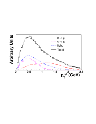
Figure 22: $p_{T}^{\mbox{\scriptsize rel}}$ distribution of muons in taggable jets. The superimposed histograms represent the contribution of simulated $b\rightarrow\mu X$ (dashed), $c\rightarrow\mu X$ (dotted), light quark jets (dash-dotted), and their sum (solid histogram). The template fit employed the method described in Ref. [27].

The requirement $p_{T}^{\mbox{\scriptsize rel}}>0.5\mbox{ GeV}$ is chosen in order to have a similar efficiency for $c$- and light-quark jets, so that the application of this requirement affects the flavor composition of the background jets only modestly. Correction factors $\kappa_{b}$ and $\kappa_{cl}$ are determined for signal and background jets by dividing the efficiency for jets satisfying both criteria by the product of the efficiencies for jets satisfying the individual criteria. They are shown in Figs. 23 and 24 for the L2 and Tight operating points, respectively.

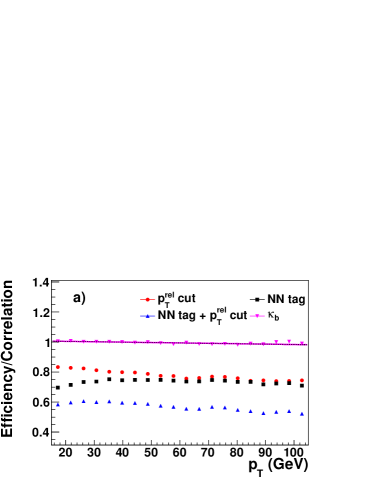
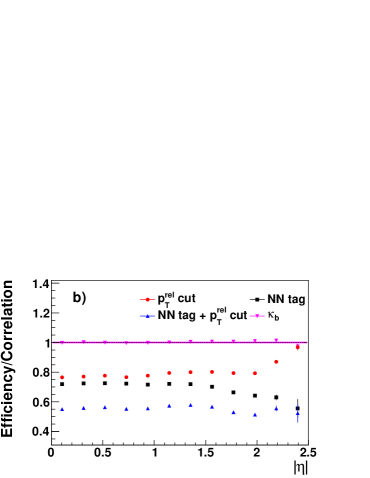
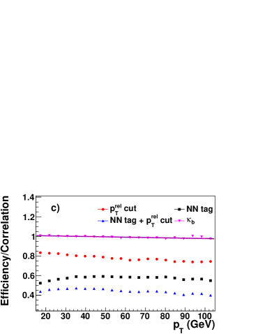
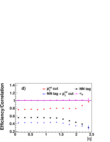
Figure 23: (a): the efficiency of the $p_{T}^{\mbox{\scriptsize rel}}$ requirement (circles), the L2 NN tagger (squares), the AND of the NN tag and $p_{T}^{\mbox{\scriptsize rel}}$ requirement (up triangles), and the correlation factor $\kappa_{b}$ (down triangles and fit), measured in the $b\rightarrow\mu X$ MC sample in the jet $p_{T}$ projection. (b): same in the $|\eta|$ projection. (c) and (d): same for the Tight NN tagger in the jet $p_{T}$ and $|\eta|$ projection, respectively. The fit uncertainties are too small to be visible in this figure.

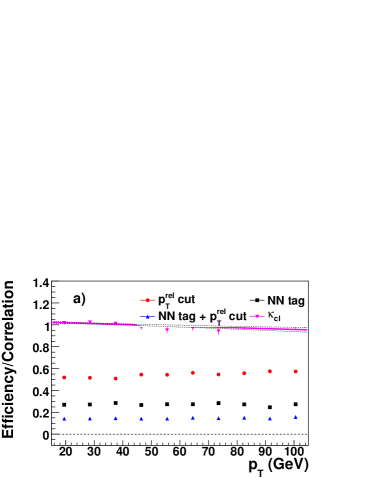
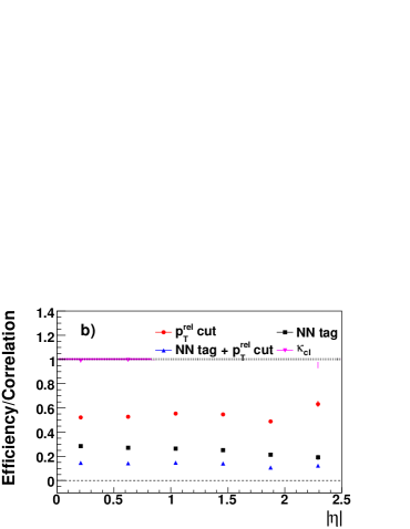
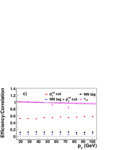
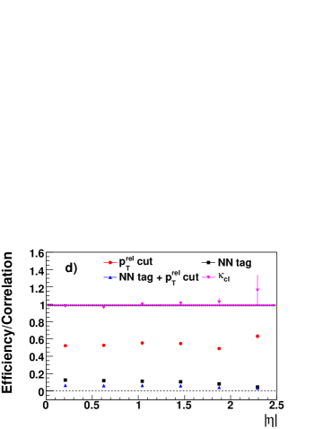
Figure 24: (a): the efficiency of the $p_{T}^{\mbox{\scriptsize rel}}$ requirement (circles), the L2 NN tagger (squares), the AND of the NN tag and $p_{T}^{\mbox{\scriptsize rel}}$ requirement (up triangles), and the correlation factor $\kappa_{cl}$ (down triangles and fit), measured in the $cl\rightarrow\mu X$ MC sample in the jet $p_{T}$ projection. (b): same in the $|\eta|$ projection. (c) and (d): same for the Tight NN tagger in the jet $p_{T}$ and $|\eta|$ projection, respectively. The dotted lines represent the fit uncertainties.

As indicated above, the application of the away side tag is not a priori expected to be correlated with the other two criteria. This hypothesis has been verified explicitly in the simulation for the correlation with the $p_{T}^{\mbox{\scriptsize rel}}$ requirement. The lifetime tagging requirements applied to both jets, however, could be correlated by the fact that they involve the same primary vertex. The corresponding correction factors are evaluated in the same way as $\kappa_{b}$ and $\kappa_{cl}$. They are denoted $\beta$ for $b$ jets and $\alpha$ for background jets.

In addition to increasing the $b$-jet fraction of the data sample, the application of the away-side tag modifies the flavor composition of the background sample, as the charm tagging efficiency is expected to be significantly higher than that for light-flavor jets. This causes a dependence of $\alpha$ on the physics assumptions made in the MC event generators (in which charm and light-flavor QCD samples are added weighted by their respective production cross sections to yield a sample of $cl$ jets). Fortunately, it turns out that the uncertainty on $\alpha$ affects the $b$-tagging efficiency only marginally. The factors $\alpha$ and $\beta$ are shown in Figs. 25 and 26, respectively, for the L2 and Tight operating points.

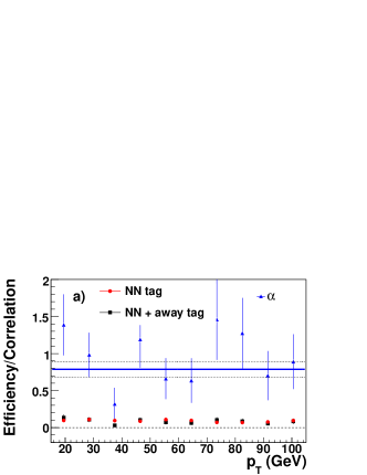
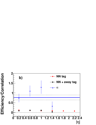
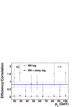
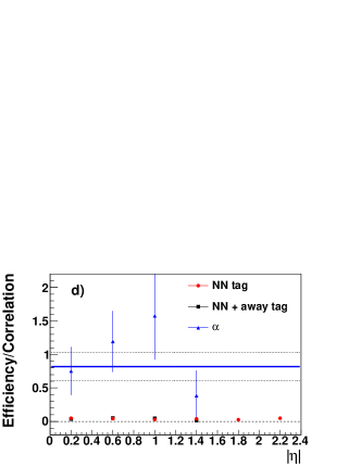
Figure 25: (a): the L2 NN tagging efficiency (circles), the tagging efficiency after an away-tag requirement (squares), and their ratio, $\alpha$ (up triangles and fit) in the $cl\rightarrow\mu X$ MC sample as a function of jet $p_{T}$. (b): same as a function of $|\eta|$. (c) and (d): same for the Tight NN tagger as a function of jet $p_{T}$ and $|\eta|$, respectively. The fit uncertainty on $\alpha$ is represented by the dotted lines.

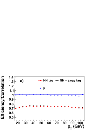
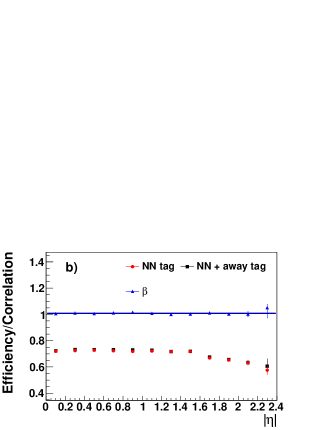
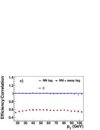
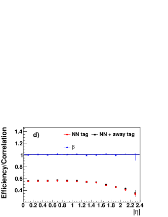
Figure 26: (a): the L2 NN tagging efficiency (circles), the tagging efficiency after an away-tag requirement (squares), and their ratio, $\beta$ (up triangles and fit) in the $b\rightarrow\mu X$ MC sample as a function of jet $p_{T}$. (b): same as a function of $|\eta|$. (c) and (d): same for the Tight NN tagger as a function of jet $p_{T}$ and $|\eta|$, respectively. The fit uncertainty on $\beta$ is too small to be visible in this figure.

8.3.3 SystemD equations

Denoting the criteria used in SystemD as $l$ for the lifetime tagging criterion, $m$ for the $p_{T}^{\mbox{\scriptsize rel}}$ requirement, and $b$ for the away-side tag, with the notation for the correction factors as above, and with $f_{0}$ and $f_{1}$ of Eq. 9 renamed to $f_{b}$ and $f_{cl}$, respectively, the final system to solve is therefore:

$$\begin{array}[]{lclcl}f_{b}&+&f_{cl}&=&1\\ f_{b}\varepsilon_{b}^{l}&+&f_{cl}\varepsilon_{cl}^{l}&=&Q^{l}\\ f_{b}\varepsilon_{b}^{m}&+&f_{cl}\varepsilon_{cl}^{m}&=&Q^{m}\\ f_{b}\varepsilon_{b}^{b}&+&f_{cl}\varepsilon_{cl}^{b}&=&Q^{b}\\ f_{b}\kappa_{b}\varepsilon_{b}^{l}\varepsilon_{b}^{m}&+&f_{cl}\kappa_{cl}\varepsilon_{cl}^{l}\varepsilon_{cl}^{m}&=&Q^{l,m}\\ f_{b}\varepsilon_{b}^{m}\varepsilon_{b}^{b}&+&f_{cl}\varepsilon_{cl}^{m}\varepsilon_{cl}^{b}&=&Q^{m,b}\\ f_{b}\beta\varepsilon_{b}^{b}\varepsilon_{b}^{l}&+&f_{cl}\alpha\varepsilon_{cl}^{b}\varepsilon_{cl}^{l}&=&Q^{b,l}\\ f_{b}\kappa_{b}\beta\varepsilon_{b}^{l}\varepsilon_{b}^{m}\varepsilon_{b}^{b}&+&f_{cl}\kappa_{cl}\alpha\varepsilon_{cl}^{l}\varepsilon_{cl}^{m}\varepsilon_{cl}^{b}&=&Q^{l,m,b}\end{array}$$ (14)

As already mentioned in Sec. 8.2, the SystemD method leads to a set of nonlinear equations, and two possible solutions exist for the quantity of interest, the $b$-tagging efficiency. The ambiguity between these two solutions is resolved using the a priori knowledge that the efficiency of each selection criterion for $b$ jets should be higher than for background jets: $\varepsilon_{b}^{l,m,b}>\varepsilon_{cl}^{l,m,b}$.

8.4 Further corrections

The $b$-tagging efficiency obtained with the SystemD method is valid for jets with a semimuonic decay of the $b$ hadron. To obtain the efficiency for inclusive jets not biased by the requirement of such a decay, a correction is determined using a sample of simulated $b$ jets with $b$ hadrons decaying inclusively or as $b\rightarrow\mu X$. The final efficiency is then defined as

$$\varepsilon^{\mbox{\scriptsize data}}_{b}=\frac{\varepsilon^{\mbox{\scriptsize data}}_{b\rightarrow\mu X}\cdot\varepsilon^{\mbox{\scriptsize MC}}_{b}}{\varepsilon^{\mbox{\scriptsize MC}}_{b\rightarrow\mu X}}=\mbox{SF}_{b}\cdot\varepsilon^{\mbox{\scriptsize MC}}_{b}\;,$$ (15)

where $\mbox{SF}_{b}=\varepsilon^{\mbox{\scriptsize data}}_{b\rightarrow\mu X}/\varepsilon^{\mbox{\scriptsize MC}}_{b\rightarrow\mu X}$ is the data-to-simulation efficiency scale factor, and $\varepsilon^{\mbox{\scriptsize data}}_{b\rightarrow\mu X}$ is identical to the quantity denoted as $\varepsilon^{t}_{b}$ in Eq. 14. The tagging efficiency for $c$-quark jets is not measured in data. It is assumed that the data-to-simulation scale factor is identical for $b$ and $c$ jets. The $c$-jet tagging efficiency is then derived from the simulation as

$$\varepsilon^{\mbox{\scriptsize data}}_{c}=\mbox{SF}_{b}\cdot\varepsilon^{\mbox{\scriptsize MC}}_{c}.$$ (16)

8.5 Tagging efficiency parametrization

The tagging efficiencies are parametrized in terms of the $p_{T}$ and $\eta$ of the jets. As the use of the SystemD method requires high statistics to obtain stable solutions, it is not possible to extract a proper 2D parametrization. Instead, it is assumed that the dependence on these variables can be factorized:

$$\varepsilon(p_{T},\eta)=\frac{1}{\varepsilon_{\mbox{\scriptsize all}}}\cdot\varepsilon(p_{T})\cdot\varepsilon(|\eta|),$$ (17)

where $\varepsilon_{\mbox{\scriptsize all}}$ is the efficiency for the entire sample, and

$$\varepsilon(p_{T}) = \frac{c}{1+ae^{-bp_{T}}},$$ (18)

$$\varepsilon(|\eta|) = d+e|\eta|+f|\eta|^{2}+g|\eta|^{3}+h|\eta|^{4},$$

where $a$ – $h$ are fit parameters.

The data $b$-jet NN tagging efficiency calculated using the SystemD method is shown in Fig. 27, along with the simulated semimuonic $b$-jet efficiency and $\mbox{SF}_{b}$. The inclusive $b$-jet efficiencies, $\varepsilon_{b}$, measured in data and in simulated events are shown in Fig. 28. The corresponding plots for $c$ jets are shown in Fig. 29.

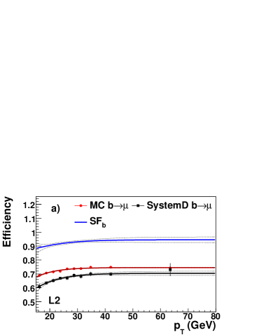
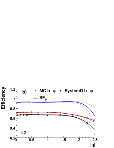
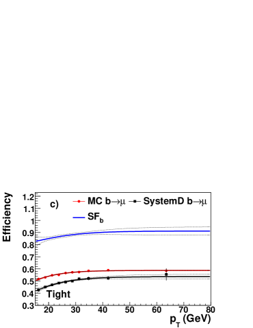
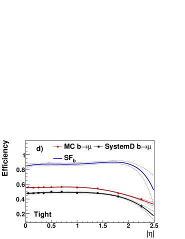
Figure 27: (a): the L2 NN tagger scale factors (line) and the data (squares) and MC (circles) semimuonic $b$-jet efficiencies as a function of jet $p_{T}$. (b): same as a function of jet $|\eta|$. (c) and (d): same for the Tight NN tagger, as a function of jet $p_{T}$ and $|\eta|$, respectively. The functions used for the parametrization are outlined in the text and the dotted curves represent the $\pm 1\sigma$ statistical uncertainty.

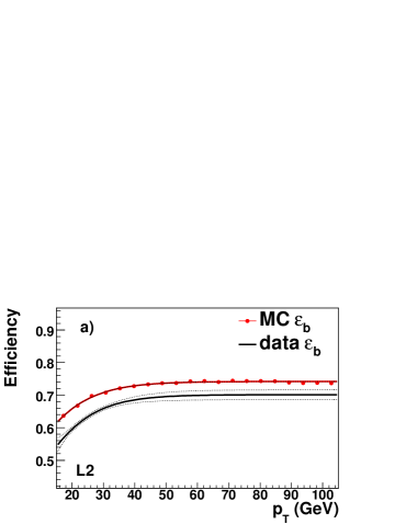
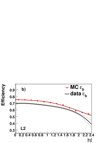
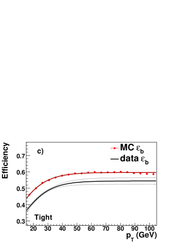
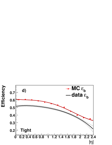
Figure 28: (a): the L2 NN tagger inclusive $b$-jet efficiency in both data (line) and MC (circles) as a function of jet $p_{T}$. (b): same as a function of jet $|\eta|$. (c) and (d): same for the Tight NN tagger, as a function of jet $p_{T}$ and $|\eta|$, respectively. The dotted lines represent the fit uncertainty, which is almost entirely inherited from the uncertainty on the scale factor. The functions used for the parametrization are outlined in the text.

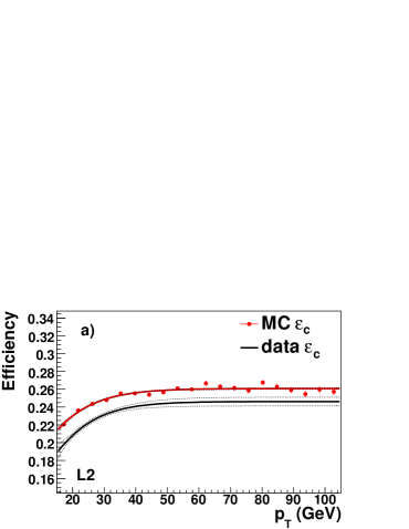
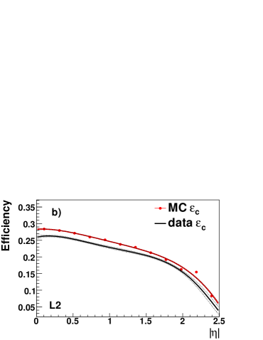
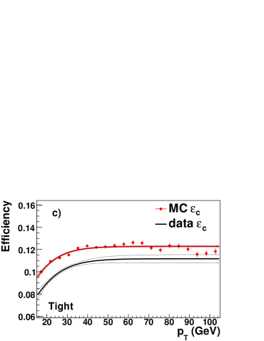
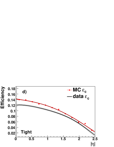
Figure 29: (a): the L2 NN tagger inclusive $c$-jet efficiency in both data (line) and MC (circles) as a function of jet $p_{T}$. (b): same as a function of jet $|\eta|$. (c) and (d): same for the Tight NN tagger, as a function of jet $p_{T}$ and $|\eta|$, respectively. The dotted lines represent the fit uncertainty, which is almost entirely inherited from the uncertainty on the scale factor. The functions used for the parametrization are outlined in the text.

8.6 Systematic uncertainties

Uncertainties on the resulting efficiencies arise from the following sources: the SystemD calculations (due to uncertainties on the correction factors as well as limited data statistics), the dependence of the efficiencies on the simulated samples, and possible imperfections in their chosen parametrization including the assumption of factorization in Eq. 17. These uncertainties are discussed below.

8.6.1 SystemD uncertainties

The correction factors $\alpha$, $\beta$, $\kappa_{b}$ and $\kappa_{cl}$ (Sec. 8.3) are evaluated using simulated events, and have non-zero statistical uncertainties. The effect of these is evaluated by repeating the SystemD computations with the parametrization of each individual factor shifted by its statistical uncertainty, while all other correction factors are fixed to their nominal values; the resulting changes in the computed efficiency are interpreted as systematic uncertainties. The effect of the choice of minimum $p_{T}^{\mbox{\scriptsize rel}}$ requirement in the SystemD calculations is evaluated by varying it between 0.3 GeV and 0.7 GeV. The total relative systematic uncertainty associated with the SystemD correction factors is estimated by adding the individual contributions in quadrature, and varies between 1.3% and 1.7% for the different operating points. As an illustration, the results of this procedure when solving SystemD for the entire sample are summarized in Table 3 for the NN L2 and Tight operating points.

For each bin in $\eta$ and $p_{T}$, the SystemD systematic uncertainty for that bin is added in quadrature with the statistical uncertainty resulting from the SystemD fit. This yields an overall uncertainty, referred to as “statistical uncertainty” below, with which the efficiency is known for each bin, and which is used in the fitting of the parametrized curves in $p_{T}$ and $|\eta|$.

The relative combined statistical and systematic uncertainties as a function of $p_{T}$ and $|\eta|$ are calculated by evaluating

$$\Delta\varepsilon^{+}(p_{T},|\eta|)=\frac{\varepsilon^{+1\sigma}(p_{T})\cdot\varepsilon^{+1\sigma}(|\eta|)}{\varepsilon^{+1\sigma}_{\mbox{\scriptsize all}}}-\frac{\varepsilon(p_{T})\cdot\varepsilon(|\eta|)}{\varepsilon_{\mbox{\scriptsize all}}},$$ (19)

where the $+1\sigma$ quantities are the fluctuations upward by one standard deviation of the quantities introduced in Eq. 17. This is also repeated with the downward fluctuations, and the larger deviation is assigned as the uncertainty.

	L2	Tight
Efficiency	65.9%	47.6%
$\alpha$	0.0%	0.0%
$\beta$	0.2%	0.6%
$\kappa_{b}$	0.7%	1.2%
$\kappa_{cl}$	0.3%	0.2%
$p_{T}^{\mbox{\scriptsize rel}}$	1.0%	0.7%
SystemD Total	1.3%	1.5%

Table 3: NN tagger efficiencies for the complete data sample, and relative systematic uncertainties originating from the SystemD method. The total systematic uncertainty is determined by adding the individual uncertainties in quadrature.

8.6.2 Efficiency parametrization and sample dependence uncertainty

Both the parametrization and MC sample dependence systematic uncertainties, which result from the use of efficiencies derived from generic combined samples of simulated $b$, $c$, and muonic $b$ jets, are quantified in one measurement. This is done by comparing the relative difference between the actual and predicted numbers of tags in various bins in $p_{T}$ and $\eta$, and for each of the simulated samples used to construct the efficiencies. This effectively constitutes a closure test, and a total uncertainty is determined from the spread of the relative differences.

In detail, the relative differences are calculated as a function of $p_{T}$ in three $|\eta|$ ranges denoted CC ($|\eta|<1$), ICR ($1<|\eta|<1.8$), and EC ($|\eta|>1.8$). The relative differences are histogrammed weighted by the number of actual tags in the region. The RMS widths of the resulting distributions are used to quantify the total uncertainty on each of the efficiencies. The relative uncertainty determined by this method ranges from 1.2% for the loosest operating point to 3.5% for the tightest operating point for the inclusive $b$-jet efficiency, and from 2.4% to 4.0% for the inclusive $c$-jet efficiency.

8.6.3 Total systematic uncertainty

Total systematic uncertainties are assigned to all bins of $p_{T}$ and $\eta$ for $\varepsilon_{b}$, $\varepsilon_{c}$, and SF_b. They are calculated as detailed below and are shown in Table 4 for the L2 and Tight NN operating points.

SF_b:

The closure test uncertainty for the $b\rightarrow\mu X$ efficiency.

$\varepsilon_{b}$:

The SF systematic uncertainty added in quadrature with the closure test uncertainty for the $b$-jet efficiency.

$\varepsilon_{c}$:

The SF systematic uncertainty added in quadrature with the closure test uncertainty for the $c$-jet efficiency.

The systematic uncertainties for $\varepsilon_{b}$ range from $\pm 1.9\%$ to $\pm 4.8\%$, for $\varepsilon_{c}$ from $\pm 2.8\%$ to $\pm 5.2\%$, and for $\mbox{SF}_{b}$ from $\pm 1.4\%$ to $\pm 3.4\%$ for the loosest to tightest working points.

Uncertainty	L2	Tight
MC $b\rightarrow\mu X$	2.4%	3.5%
MC $b$	1.8%	2.8%
MC $c$	2.9%	3.9%
SFb	2.4%	3.5%
$\varepsilon_{b}$	3.0%	4.5%
$\varepsilon_{c}$	3.8%	5.2%

Table 4: Total relative systematic uncertainties on the MC sample parametrizations, and their effect on $\varepsilon_{b}$, $\varepsilon_{c}$, and $\mbox{SF}_{b}$.

The total uncertainties are computed by adding in quadrature the systematic and the statistical uncertainties (which include the SystemD systematic uncertainties, as detailed in Sec. 8.6.1). They are shown for $\mbox{SF}_{b}$, $\varepsilon_{b}$, and $\varepsilon_{c}$ in Fig. 30 for the L2 and Tight operating points. The relative uncertainty increases rapidly at high $\eta$ due to limited statistics in that region and because the value of the scale factor drops rapidly for $|\eta|>2$.

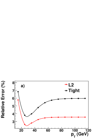
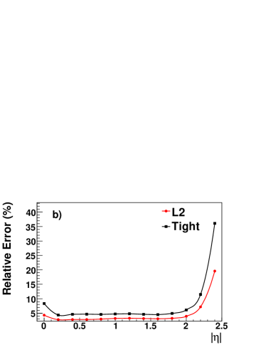
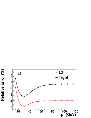
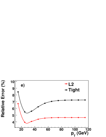
Figure 30: The total relative uncertainty (combined systematic and statistical) for the Scale Factor ($\mbox{SF}_{b}$) (a, b), $\varepsilon_{b}$ (c, d) and $\varepsilon_{c}$ (e, f) as a function of $p_{T}$ (a, c, e) when $\eta=1.2$, and $\eta$ (b, d, f) when $p_{T}=45\mbox{ GeV}$.

9 Fake Rate Determination

The determination of the light-flavor mistag rate (where “light” stands for $uds$-quark or gluon jets) or fake rate relies on the notion that in the absence of long-lived particles such as $V^{0}$s (see Sec. 3.3), reconstructed high-impact parameter tracks or displaced vertices reconstructed in light-flavor jets result from resolution and misreconstruction effects. These effects are expected to lead to tracks with negative impact parameters (see Sec. 5 for the impact parameter sign convention used) and displaced vertices with negative decay lengths as often as to positive impact parameters and decay lengths. Barring incorrectly assigned negative impact parameter signs (which may occur whenever a jet and a track are nearly aligned in azimuth, and which is important for long-lived particles), using such negative impact parameter tracks and negative decay length vertices should provide a reasonable estimate of the fake rate.

9.1 Data sample

To minimize the impact of incorrectly attributed impact parameter signs, the fake rate is determined in an inclusive jet sample with low heavy flavor content. Two samples are used for this purpose:

• A sample consisting of events selected by requiring at least one electron candidate with $p_{T}>4\mbox{ GeV}$ and with low missing transverse energy, $\hbox to0.0pt{\hbox to7.95831pt{\hfil/\hfil}\hss}E_{T}<10\mbox{ GeV}$, and referred to below as the EM sample. As in Sec. 8.3, at least one trigger without lifetime bias is required. Most of the electron candidates are jets that deposit a large fraction of their energy in the EM section of the calorimeter. This may reduce the heavy flavor content of the sample, as the fraction of a jet’s energy deposited through electromagnetic processes depends on the jet flavor. This bias is removed by only considering jets whose distance to the nearest identified EM cluster is $\Delta\mathcal{R}>0.4$. After these requirements, the EM sample contains 106 million taggable jets.

• An inclusive jet sample (referred to in the following as the QCD sample) consisting of all events collected using jet triggers. It contains 154 million taggable jets. For consistency, jets in the vicinity of identified EM clusters are not considered in this sample either. Since trigger requirements should not bias such jets in this sample, the effect of this removal should be small and will be evaluated below.

These two samples are combined (referred to as the COMB sample) for most studies; their comparison allows a systematic uncertainty associated with the choice of a particular sample to be estimated. The $p_{T}$ and $\eta$ distributions in these samples, after the taggability requirement, are compared in Figure 31. The main difference is an increased high-$p_{T}$ content in the QCD sample due to trigger effects.

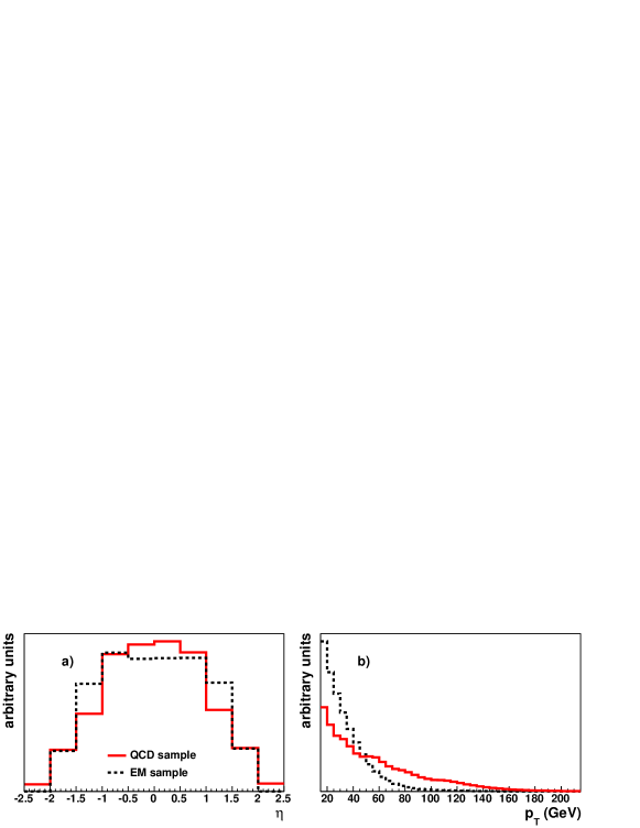
Figure 31: Jet $\eta$ (a) and $p_{T}$ (b) distributions in the QCD and EM data samples.

9.2 Negative tag rate

The use of negative impact parameter tracks and negative decay length displaced vertices is rather straightforward: the algorithms providing the NN input variables listed in Sec. 7.1.1 need only minor modifications in order to provide “negative” equivalents of these variables, called Negative Tag (NT) results. The NN output is then recomputed using the NT values rather than the original ones, and the fraction of jets tagged in this modified fashion represents the negative tag rate. The NN input NT results are computed as follows:

CSIP:

The $\mathcal{N}_{\mbox{\scriptsize CSIP}}$ variable is recalculated using tracks with negative instead of positive impact parameter significance to obtain the “strong classifier” numbers of tracks $N_{3s}$ and $N_{2s}$ (see Sec. 6).

JLIP:

The Jet Lifetime Probability $\mathcal{P}_{\mbox{\scriptsize JLIP}}$ is recomputed using only tracks with negative rather than positive impact parameter significance.

SVT:

In this case, no additional computation is necessary. Instead of the highest (positive) decay length significance, the most negative decay length significance displaced vertices (for both the SuperLoose and Loose algorithm versions discussed in Sec. 4) are used to supply the SVT-related NN variables.

Like the $b$-jet efficiency, the fake rate and negative tag rate are parametrized as functions of a jet’s kinematical ($p_{T}$, $|\eta|$) variables. However, in contrast to the efficiency, the data shows that the dependence of the NT rate on jet $p_{T}$ and $|\eta|$ cannot be factorized into a dependence on $p_{T}$ multiplied by a dependence on $|\eta|$. Instead, it is parametrized as a function of jet $p_{T}$ in three regions: $0<|\eta|<1.0$ (CC), $1.0<|\eta|<1.8$ (ICR), and $1.8<|\eta|<2.5$ (EC). In each region, the $p_{T}$ dependence is parametrized using a quadratic polynomial. The negative tag rate parametrizations in the three $|\eta|$ regions are shown in Fig. 32 for the L2 and Tight operating points.

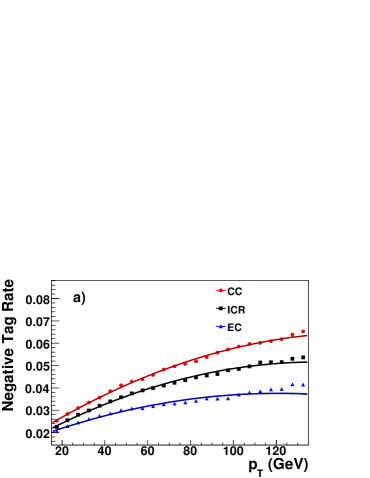
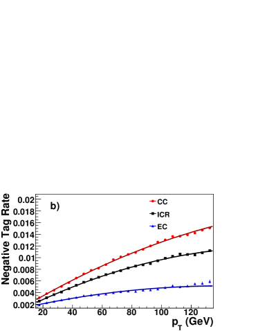
Figure 32: The NT rate parametrization for the COMB sample in the CC (circles), ICR (squares), and EC (triangles) for the L2 (a) and Tight (b) operating points. The negative tag rate is parametrized with a second order polynomial. The fit uncertainty is too small to be visible in this figure.

9.3 Corrections

The NT rate is not a perfect approximation of the fake rate. Corrections for the following effects are applied:

• The presence of heavy flavor jets increases the NT rate, primarily due to tracks that originate from the decay of long-lived particles and are (mistakenly) assigned a negative impact parameter sign. As no method is available to estimate this effect on data, QCD events simulated using the Pythia event generator are used instead. This results in a correction factor $F_{\mbox{\scriptsize hf}}=\varepsilon^{\mbox{\scriptsize NT}}_{\mbox{\scriptsize QCD,light}}/\varepsilon^{\mbox{\scriptsize NT}}_{\mbox{\scriptsize QCD,all}}$, i.e., the ratio of NT rates with and without the presence of heavy flavor jets in these simulated events.

• The $V^{0}$ removal algorithm (see Sec. 3.3) is not fully efficient, so that some contribution from long-lived particles and photon conversions remains. Most of the resulting tracks will correctly be assigned positive impact parameters, and the NT rate is affected less by their presence than the fake rate. This effect is estimated using the same simulated QCD events as for the $F_{\mbox{\scriptsize hf}}$ factor, leading to a correction factor $F_{\mbox{\scriptsize lf}}=\varepsilon^{\mbox{\scriptsize PT}}_{\mbox{\scriptsize QCD,light}}/\varepsilon^{\mbox{\scriptsize NT}}_{\mbox{\scriptsize QCD,light}}$, i.e., the ratio of the positive- and negative-tag rates in the simulated light-flavor events.

Finally, the fake rate $\varepsilon_{\mbox{\scriptsize light}}$ is estimated as the NT rate measured in data, $\varepsilon^{\mbox{\scriptsize NT}}_{\mbox{\scriptsize data}}$, corrected for the above effects:

$$\varepsilon_{\mbox{\scriptsize light}}=\varepsilon^{\mbox{\scriptsize NT}}_{\mbox{\scriptsize data}}\cdot F_{\mbox{\scriptsize hf}}\cdot F_{\mbox{\scriptsize lf}}.$$ (20)

The jet $p_{T}$ dependences of $F_{\mbox{\scriptsize hf}}$ and $F_{\mbox{\scriptsize lf}}$ are shown in Fig. 33 for the L2 and Tight operating points. The estimated light quark tagging efficiencies $\varepsilon_{\mbox{\scriptsize light}}$ for the L2 and Tight operating points are shown in Fig. 34. Both the negative and positive tag rates for light-flavor jets increase with increasing jet $p_{T}$, for two reasons: (i) the multiplicity of long-lived particles and their average decay length increase; and (ii) jets become more collimated, with the resulting higher hit density leading to a larger number of wrongly reconstructed high-impact parameter tracks.

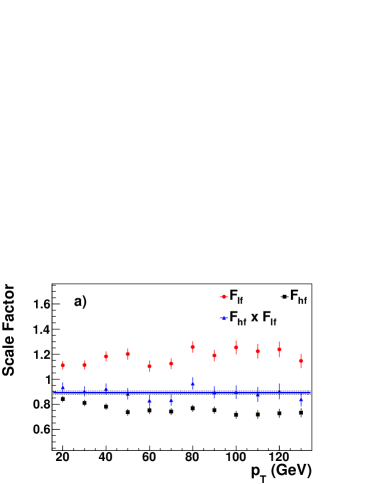
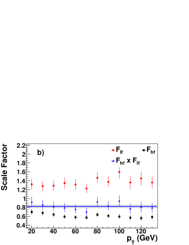
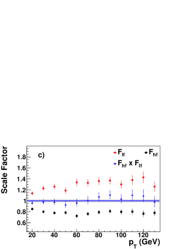
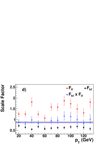
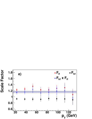
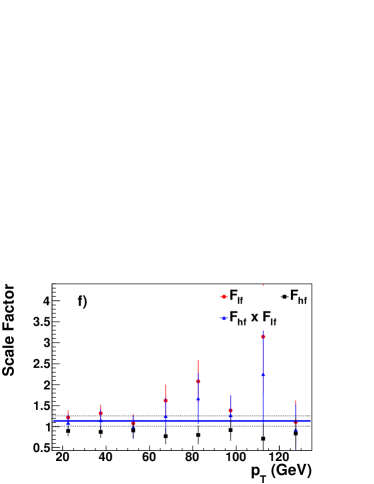
Figure 33: The light jet asymmetry correction, $F_{\mbox{\scriptsize lf}}$ (circles), heavy flavor correction, $F_{\mbox{\scriptsize hf}}$ (squares), and total negative tag correction (triangles) in the CC (a, b), ICR (c, d) and EC regions (e, f) for the L2 (a, c, e) and Tight (b, d, f) operating points. The solid and dotted lines indicate the fit of the total correction factor and its uncertainty, respectively.

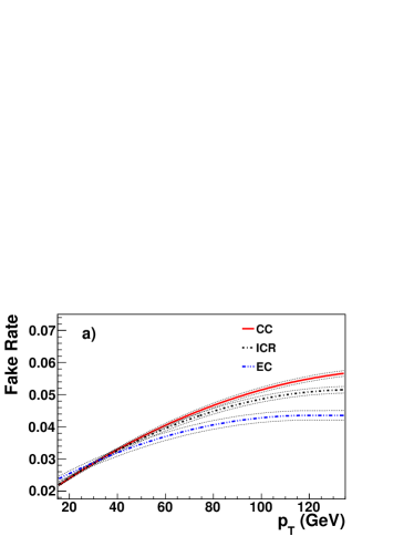
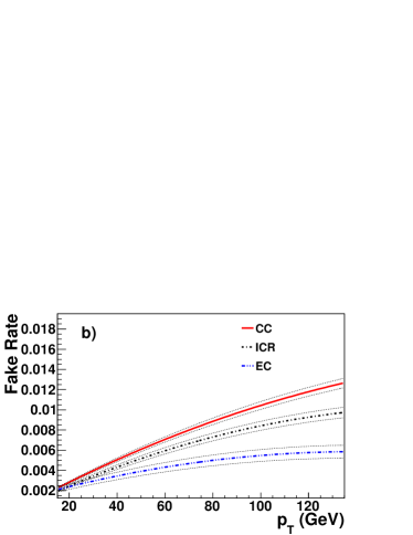
Figure 34: The estimated light quark tagging efficiency parametrized in the CC (continuous line), ICR (dot-dashed line) and EC (dot-dot-dashed line) for the L2 (a) and Tight (b) operating points. The dotted black lines represent the fit uncertainty.

9.4 Systematic uncertainties

The use of a particular sample (in this case, the combination of the QCD and EM multijet samples) to provide a “universal” estimate of the NT rate needs to be validated. To this end, the ratio of the NT rates as measured in the separate QCD and EM samples is determined as a function of the kinematical variables and is shown in Fig. 35 for the L2 and Tight operating points.

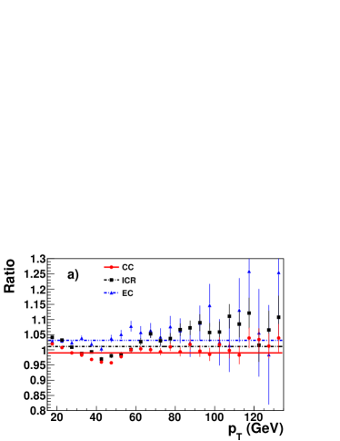
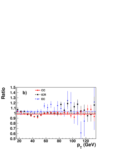
Figure 35: The ratio of the EM and QCD negative tag rates for the L2 (a) and Tight (b) operating points in the CC (circles, continuous line), ICR (squares, dot-dashed line), and EC regions (triangles, dot-dot-dashed line).

A corresponding systematic uncertainty is calculated from a constant fit to the EM/QCD NT rate ratio. Half the difference between the fit value and unity is taken as the systematic uncertainty, or if the ratio is consistent with unity within the fit uncertainty scaled by $\sqrt{\chi^{2}/N_{\mathrm{dof}}}$, this scaled fit uncertainty is taken as the uncertainty. The relative uncertainty ranges from 0.2% to 1.3% in the CC, 0.3% to 0.7% in the ICR and 1.2% to 3.1% in the EC from the loosest to tightest operating points.

In addition, the effect of removing jets in the vicinity of EM clusters in the QCD sample needs to be taken into account. The NT rate in the QCD sample with the jets removed is slightly lower than in the full QCD sample. The effect is small, ranging from 0.2% for the loosest to 1% for the tightest operating point, and does not depend on jet $p_{T}$. A systematic uncertainty is assigned in the same way as that for the difference between the EM and QCD samples, and ranges from 0.1% to 0.6% in the CC, 0.1% to 0.3% in the ICR, and 0.1% to 0.7% in the EC from the loosest to tightest operating points.

To test the parametrization of the NT rate in the three $|\eta|$ regions a comparison is made between the number of tags found by the tagger and its prediction from the parametrized NT rate. A systematic uncertainty is again calculated from a constant fit to the ratio of the actual and predicted number of tags, following the same procedure as the EM/QCD sample comparison. The systematic uncertainty ranges from 0.1% to 0.3% in the CC/ICR and from 0.1% to 0.7% in the EC from the loosest to tightest operating points.

The $F_{\mbox{\scriptsize hf}}$ correction factor depends on the assumed $b$- and $c$-fractions in the multijet data sample. In turn, these depend on the cross sections for QCD heavy flavor production. To estimate the uncertainty on $F_{\mbox{\scriptsize hf}}$, the fraction of $b$ ($c$) jets is varied from its default value of 2.6% (4.6%) by 50% (relative). Given that the individual $b$- and $c$-production mechanisms are very similar, these fractions are varied coherently. The total uncertainties from varying the fraction of $b$ ($c$) jets ranges from 2.8% (1.6%) for the loosest to 19.5% (4.7%) for the tightest operating point in the CC/ICR and from 1.0% (0.7%) to 6.7% (3.5%) in the EC regions.

The total uncertainty on the fake tag rate is given by adding in quadrature the systematic contributions (as discussed above) for the appropriate region to the statistical uncertainty, estimated as the difference between the fake tag rate central value and one standard deviation fit curves. The dominant contribution is the systematic one. The combined relative systematic uncertainty ranges from 5.9% (for the loosest operating point) to 23.1% (for the tightest operating point) in the CC region, from 4.8% to 24.2% in the ICR region, and from 2.2% to 10.0% in the EC region. A more detailed breakdown of the systematic uncertainties is shown in Tables 5 and 6 for the L2 and Tight operating points, respectively.

Region	CC	ICR	EC
Parametrization	0.1%	0.1%	0.1%
EM/QCD	0.5%	0.5%	1.6%
EM veto	0.2%	0.1%	0.1%
$c$ fraction	3.7%	3.3%	1.3%
$b$ fraction	7.3%	6.4%	2.2%
Total	11.0%	9.7%	3.8%

Table 5: Fake tag rate relative systematic uncertainties for the L2 NN operating point.

Region	CC	ICR	EC
Parametrization	0.1%	0.2%	0.4%
EM/QCD	1.0%	0.5%	1.6%
EM veto	0.5%	0.2%	0.5%
$c$ fraction	4.5%	4.5%	1.4%
$b$ fraction	14.3%	13.8%	4.2%
Total	18.8%	18.3%	5.9%

Table 6: Fake tag rate relative systematic uncertainties for the Tight NN operating point.

10 Summary and Conclusion

Several techniques to identify $b$ jets exploiting the long lifetime of $b$ hadrons have been discussed in this article. Compared to the use of individual $b$-jet tagging algorithms, the combination of their results in an artificial neural network leads to a considerable improvement in performance.

This performance needs to be calibrated using the actual collider data, as the simulation cannot be expected to reproduce the performance of the detector in all aspects relevant to $b$-jet tagging. The calibration methods described employ QCD jet samples, and therefore can make use of ample statistics at low jet $p_{T}$.

• Starting from the further requirement of a muon-jet association, the SystemD method allows the determination of the $b$-jet tagging efficiency, with minimal input from simulation, even in the presence of an a priori unknown background.

• The determination of the light-flavor mistag rate makes use of the fact that without such a muon requirement, the sample consists almost entirely of light-flavor jets. This method is limited by the knowledge on the remaining heavy-flavor content.

The resulting performance as measured using data, including full statistical and systematic uncertainties, is shown in Fig. 36 for all jets and for jets with $|\eta|<1.1$ and $p_{T}>30\mbox{ GeV}$.

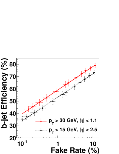
Figure 36: Data performance profile of the NN tagger as applicable to the kinematics of $Z\rightarrow b\bar{b}$ and $Z\rightarrow q\bar{q}$ events for all jets (dashed line) and for jets with $|\eta|<1.1$ and $p_{T}>30\mbox{ GeV}$ (solid line). The vertical error bars on the plot represent the total uncertainty (statistical and systematic uncertainties added in quadrature) on the performance measurements.

These tagging algorithms and calibration methods have been used in many publications of D0 Run IIa analyses. They are being refined to make use of a new layer of silicon sensors installed at even smaller distance from the beam line [28], as well as cope with the higher instantaneous luminosities common in the Run IIb data taking period that started in June 2006. The calibration methods are not specific to D0 and could be used at other experiments.

References

- [1] C. Amsler, et al., Phys. Lett. B 667 (2008) 1.
- [2] F. Abe, et al., Phys. Rev. Lett. 74 (1995) 2626.
- [3] S. Abachi, et al., Phys. Rev. Lett. 74 (1995) 2632.
- [4] V. Abazov, et al., Nucl. Instrum. Meth. A 565 (2006) 463.
- [5] S. Ahmed, et al., to be submitted to Nucl. Instrum. Meth. A.
- [6] V. Abazov, et al., Phys. Rev. Lett. 100 (2008) 192003.
- [7] V. M. Abazov, et al., Phys. Rev. Lett. 103 (2009) 092001.
- [8] R. Frühwirth, P. Kubinec, W. Mitaroff, M. Regler, Comput. Phys. Comm. 96 (1996) 189.
- [9] J. D’Hondt, P. Vanlaer, R. Frühwirth, W. Waltenberger, IEEE Trans. Nucl. Sci. 51 (2004) 2037.
- [10] G. Blazey, et al., Run II Jet Physics, in: U. Baur, R. Ellis, D. Zeppenfeld (Eds.), QCD and Weak Boson Physics in Run II, Fermilab, 1999, FERMILAB-CONF-00-092-E. arXiv:hep-ex/0005012.
- [11] D0 Collaboration, to be submitted to Phys. Rev. D.
- [12] E. Berger (Ed.), Research directions for the decade. Proceedings, 1990 Summer Study on High-Energy Physics, Snowmass, USA, June 25 - July 13, 1990, Singapore: World Scientific (1992).
- [13] A. Schwartzman, Ph.D. thesis, Universidad de Buenos Aires, FERMILAB-THESIS-2004-21 (2004).
- [14] R. Frühwirth, Nucl. Instrum. Meth. A 262 (1987) 444.
- [15] M. Mangano, et al., J. High Energy Phys. 0307 (2003) 001.
- [16] S. Greder, Ph.D. thesis, Institut de Recherches Subatomiques, Strasbourg, France, FERMILAB-THESIS-2004-28 (2004).
- [17] D. Buskulic, et al., Phys. Lett. B 313 (1993) 535.
- [18] G. Borisov, C. Mariotti, Nucl. Instrum. Meth. A 372 (1996) 181.
- [19] D. Knuth, The Art of Computer Programming, Vol. 2, Addison-Wesley, 1969.
- [20] A. Khanov, Ph.D. thesis, University of Rochester, Rochester, New York, FERMILAB-THESIS-2004-15 (2004).
- [21] C. Bishop, Neural Networks for Pattern Recognition, Oxford University Press, 1996.
- [22] T. Scanlon, Ph.D. thesis, Imperial College London, London, UK, FERMILAB-THESIS-2006-43 (2006).
- [23] http://www.root.cern.ch/. The training method chosen is the Broyden-Fletcher-Goldfarb-Shanno (BFGS) method.
- [24] T. Sjöstrand, et al., Comput. Phys. Comm. 135 (2001) 238.
- [25] K. Hornik, et al., Neural Networks 2 (1989) 359.
- [26] B. Clément, Ph.D. thesis, Institut de Recherches Subatomiques, Strasbourg, France, FERMILAB-THESIS-2006-06 (2006).
- [27] R. Barlow, C. Beeston, Comput. Phys. Comm. 77 (1993) 219.
- [28] R. Angstadt, et al., The Layer 0 Inner Silicon Detector of the D0 Experiment, submitted to Nucl. Instrum. Meth. A, arXiv:0911.2522 [physics.ins-det].