Sparse Channel Separation using Random Probes

Abstract

This paper considers the problem of estimating the channel response (or Green’s function) between multiple source-receiver pairs. Typically, the channel responses are estimated one-at-a-time: a single source sends out a known probe signal, the receiver measures the probe signal convolved with the channel response, and the responses are recovered using deconvolution. In this paper, we show that if the channel responses are sparse and the probe signals are random, then we can significantly reduce the total amount of time required to probe the channels by activating all of the sources simultaneously. With all sources activated simultaneously, the receiver measures a superposition of all the channel responses convolved with the respective probe signals. Separating this cumulative response into individual channel responses can be posed as a linear inverse problem.

We show that channel response separation is possible (and stable) even when the probing signals are relatively short in spite of the corresponding linear system of equations becoming severely underdetermined. We derive a theoretical lower bound on the length of the source signals that guarantees that this separation is possible with high probability. The bound is derived by putting the problem in the context of finding a sparse solution to an underdetermined system of equations, and then using mathematical tools from the theory of compressive sensing. Finally, we discuss some practical applications of these results, which include forward modeling for seismic imaging, channel equalization in multiple-input multiple-output communication, and increasing the field-of-view in an imaging system by using coded apertures.

1 Introduction

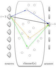
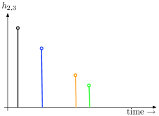
(a) (b)

Figure 1: (a) Multiple sources on left, multiple receivers on the right. The black arrow denotes the direct arrival from source $2$ to receiver $3$. The colored arrows denote the indirect arrivals caused by the different reflectors (denoted by small circles). (b) Channel response $h_{2,3}$ between source $2$ and receiver $3$.

This paper gives a theoretical treatment to the problem of channel estimation in multiple-input multiple-output (MIMO) systems. The general scenario is illustrated in Figure 1: A set of $p$ sources emit different probe signals, which then travel through different channels and are observed by $q$ receivers. We will assume that the channel between each source/receiver pair is linear and time-invariant; if source $i$ sends probe signal $\phi_{i}$, then receiver $j$ observes the convolution $\phi_{i}\star h_{i,j}$ of the probe signal with the corresponding channel response $h_{i,j}$. The goal is to estimate all of the channel responses, and to do so using the smallest total amount of probing time.

We will focus on the discrete version of this problem. We assume that each channel response $h_{i,j}$ has length $n$. If a single source $i$ emits a probe sequence $\{\phi_{i}(1),\phi_{i}(2),\ldots,\phi_{i}(m)\}$ of length $m$, receiver $j$ observes the linear convolution

$$y^{\mathrm{lin}}_{i,j}=\phi_{i}\star h_{i,j}=\begin{bmatrix}\phi_{i}(1)&0&\ldots&0\\ \phi_{i}(2)&\phi_{i}(1)&\ldots&0\\ \vdots&&&\\ \phi_{i}(n)&\phi_{i}(n-1)&\ldots&\phi_{i}(1)\\ \vdots&&&\\ \phi_{i}(m)&\phi_{i}(m-1)&\ldots&\phi_{i}(m-n+1)\\ 0&\phi_{i}(m)&\ldots&\phi_{i}(m-n+2)\\ \vdots&&&\\ 0&0&\ldots&\phi_{i}(m)\end{bmatrix}\begin{bmatrix}h_{i,j}(1)\\ h_{i,j}(2)\\ \vdots\\ h_{i,j}(n)\end{bmatrix}=:\Phi^{\mathrm{lin}}_{i}h_{i,j}.$$ (1.1)

Recovering $h_{i,j}$ from $y^{\mathrm{lin}}_{i,j}$ is a classical deconvolution problem. The inverse problem can be made very well conditioned if $\phi_{i}$ is chosen carefully; if not, then the inversion can be regularized using some type of prior information about the channel.

We will measure the cost of the channel estimation by the amount of time we spend probing the channel, which we can see is proportional to $n+m-1=O(n+m)$, the number of rows in the linear system in (1.1). From a single source, we can estimate the response to all of the receivers by emitting a single probing sequence and solving (1.1) at each receiver $j$. If there are multiple sources, then typically the sources are activated one-at-a-time. In this case, the total activation time required to estimate all of the $h_{i,j}$ becomes $O(p(n+m))$. In theory, $m$ could be made as small as we like in this situation, giving us a lower bound on the cost of $O(np)$.

In this paper, we propose and rigorously analyze an alternative strategy for estimating the channels between each source-receiver pair. Our strategy will reduce the total amount of time spent on probing the channels by activating all of the sources simultaneously. (This approach was first proposed in the context of seismic imaging in a related conference paper [28].) Now, of course, the sources will interfere with one another, and the receiver will observe a combination of each source convolved with its respective channel. With all $p$ sources active, the observations at receiver $j$ can be written as the following system of equations

$$y^{\mathrm{lin}}_{j}=\sum_{i=1}^{p}y^{\mathrm{lin}}_{i,j}=\begin{bmatrix}\Phi^{\mathrm{lin}}_{1}&\Phi^{\mathrm{lin}}_{2}&\cdots&\Phi^{\mathrm{lin}}_{p}\end{bmatrix}\begin{bmatrix}h_{1,j}\\ h_{2,j}\\ \vdots\\ h_{p,j}\end{bmatrix}=:\Phi^{\mathrm{lin}}h_{j}.$$ (1.2)

The $\Phi^{\mathrm{lin}}$ in (1.2) is the $(m+n-1)\times np$ matrix formed by concatenating the source convolution matrices $\Phi^{\mathrm{lin}}_{i}$ row-wise; the $h_{j}$ is the unknown $np$-vector consisting of the $p$ channel responses for the path between each source and receiver $j$. With all of the sources activated simultaneously, the total cost of the acquisition is $O(n+m)$, but now the channel responses are interfering with one another. The question now is how long (quantified by $m$) the probing sequences must be to reliably “untangle” the individual $h_{i,j}$ from $\Phi^{\mathrm{lin}}h_{j}$. If the probing sequences are chosen carefully and in concert with one another, the system in (1.2) will be invertible for $m\approx np$, again making the total activation time $O(np)$. If we are interested in recovering all possible channels without making any assumptions about their structure, we of course cannot have $m<np$.

We will show that if the combined channel response $h_{j}$ is sparse, then the probing sequences can be significantly shorter than $np$ if they are random. This problem, along with the tools we will deploy to solve it, is closely related to recent work in the field of compressive sensing (CS). The theory of CS basically states that vectors $x_{0}$ with $s$ non-zero components can be recovered from an underdetermined set of linear measurements $y=\Phi x_{0}$ if the the matrix $\Phi$ is sufficiently diverse (the precise technical conditions are reviewed in detail in Section 2). The essential contribution of this paper is to show that when the sequences $\{\phi_{i}(t)\}_{t}$ consist of independent and identically distributed Gaussian random variables, the matrix $\Phi^{\mathrm{lin}}$ in (1.2) meets this criterion for pulse lengths $m$ that are within a poly-logarithmic factor of the sparsity $s$. In particular, Theorems 3.1 and 3.3 combined with Proposition 2.1 shows that if the total number of significant components in $h_{j}$ is $s$, then it can be recovered from $y^{\mathrm{lin}}$ for

$$m~{}\lesssim~{}s\cdot\log^{5}(np),$$

reducing the total time the sources are activated to $O(n+s\log^{5}(np))$. When the channels are sparse, that is $s\ll np$, then the cost of acquiring all of the channels is not much more than acquiring a single channel independently. While having the sources activated simultaneously introduces “cross-talk” between the different channels, the use of different random codes by each source coupled with the sparse structure of the channels allows us to separate the cross-talk into its constituent components.

In the remainder of this section, we will discuss some applications of the channel separation problem and review recent related work. Section 2 provides an overview of sparse recovery from underdetermined linear measurements. Section 3 carefully states our main theorems, which provide a sufficient lower bound on the length of the probing signals (in relation to the number of sources, the length of the channels, and their sparsity) that allows us to robustly recover $h_{j}$ from $y^{\mathrm{lin}}$ using any number of sparse recovery algorithms. Proof of these theorems is given in Sections 4 and 5. The proofs rely heavily on estimates for random sums of rank-1 matrices, which are overviewed in the Appendix.

1.1 Applications

For further motivation, we discuss three specific scenarios in which this multichannel separation problem arises.

Seismic exploration and forward modeling. Subsurface images of the earth are formed by activating different points on the surface with acoustic sources, then measuring the response at a number of receivers locations. From these recorded responses, a 3D subsurface model of the earth (consisting of the local velocity of the propagating elastic waves) can be reconstructed using what is known as full waveform inversion (FWI). Dense samplings for the positions of the acoustic sources lead to higher resolution reconstructions, but also longer field acquisitions and more computationally intensive inversion.

The theoretical results in this paper suggest that these expenses can mitigated by activating the sources simultaneously using different random patterns. In the field, this reduces the amount of time required for the acquisition. Although the sources will interfere with one another, the individual responses can be separated afterwards by taking advantage of the sparsity of each of the channel responses. The source waveforms will have to be longer than if each of the $p$ sources were activated individually, but the net activation time across all sources is much smaller than $p$ individual channel probes.

Sparse channel separation can also reduce the amount of computation required for the inversion. The most expensive step in wavefront inversion is testing a candidate model to see how well it fits the measurements that have been collected. This so-called forward modeling simulation consists of solving an extremely large PDE. The cost of this simulation is proportional to the length of the source signals (i.e. the number of time steps required), but does not depend at all on the number of sources that are active at one time — running a simulation with a single source active costs takes just as long per time step as with many sources active. If we simulate each of the $p$ sources individually, we will need to run each simulation for $O(n)$ time for a total cost of $O(np)$ time steps (and the cost of each time step can be extremely high). If we simulate the sources simultaneously, then the number of time steps in the simulation can be $O(n+s\log^{5}(np))$. Given the results of the simulation with simultaneous active sources, we will of course have to recover the individual channel responses using some type of sparse recovery algorithm (solving the optimization program in (2.4) below, for example). But the computations required for this recovery are minor in comparison to the forward modeling simulation, especially given recent progress in optimization algorithms [15, 19, 39, 2] and the fact that the system $\Phi^{\mathrm{lin}}$ can be applied quickly using FFTs.

Source separation for seismic exploration is explored in further detail in the companion publications [28, 29].

Channel estimation in MIMO communications. When information is transmitted wirelessly, it is often the case that reflections cause there to be multiple paths from the source to the receiver. Instead of the transmitted waveform, the receiver observes a convolution of this waveform with a channel response — if the number of reflectors is small, this response is sparse. To compensate for this multipath effect, the channel is periodically estimated by having the source emit a known probing sequence that the receiver can subsequently deconvolve. If there are multiple transmitters and multiple receivers, we can save time by probing all of the channel pairs simultaneously, and separating the individual responses using sparse recovery. This approach is particularly useful when the channel is changing rapidly, a common problem in underwater acoustic communications [9].

Coded aperture imaging. In [26, 25, 24], an imaging architecture is introduced to increase the field-of-view (FOV) of a camera using coded apertures. A coded aperture is a series of small openings (apertures) whose net effect is to convolve a target image with a sequence (code) determined by the pattern in which these openings appear. Coded apertures offer a way around the classical trade-off between aperture size and image brightness; the multiple apertures overlay many copies of the image at slightly different shifts, making the image incident on the detector array “bright” and easily recovered (via deconvolution) if the aperture code is chosen carefully (e.g. the MURA patterns in [17]).

The essential idea from [24] to increase the FOV without sacrificing resolution is illustrated in Figure 2: the image is broken into $p$ subimages, each of which we would like to recover to a resolution of $n$ pixels. Rather than measuring each subimage directly, which would require a detector array of size $m=np$, we pass each image through its own coded aperture of size $m$ and these coded subimages are combined onto a detector array of size $m$. The task at hand, then, is to recover the full $np$ pixel image from these $m$ measurements.

This problem also conforms to our multichannel framework — in this case, we have $p$ sources and one receiver. Here, the known “probe signals” are the coded aperture patterns and the unknown channels $h_{i,1}$ are the different subimages. The main results of this paper say that if the entire image is approximately $s$ sparse, than the size $m$ of the detector array needs only to be only on the order of $s$ (within a log factor) rather than the full resolution $np$. If the images we are reconstructing are consecutive frames in a video sequence, the image sparsity can come from looking at the differences between consecutive frames.

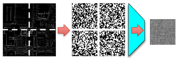
Figure 2: Sketch of the architecture proposed in [24] for increasing the field of view of a camera. The image is broken into $p$ subimages, each subimage passes through a different coded aperture, and the coded subimages are combined on the detector array. The effect of the coded aperture is to convolve the subimage with an associated code, and so (1.2) models the process mathematically.

1.2 Relationship to previous work

We have cast the multichannel separation problem as recovering a sparse vector from an underdetermined, random system of equations. This general problem has been studied extensively over the past five years under the name of compressive sensing (CS). The essential results from this field state that if we observe $y=\Phi x_{0}$, where $x_{0}$ is $s$-sparse and $\Phi$ is an $m\times N$ matrix that obeys a technical condition called the restricted isometry property (see (2.3) below), then $x_{0}$ can be recovered from $y$ even when $m\ll N$, and this recovery is stable in the presence of measurement noise, and robust against modeling error (i.e. it is effective even when $x_{0}$ is not perfectly sparse) [7, 6, 13]. Random matrices that obey this property for $m$ within a logarithmic factor of $s$ include matrices with independent entries [7, 1], matrices that have been subsampled from orthobases consisting of vectors whose energy is almost evenly distributed between their entries [33], as well as other matrices with more structured randomness [37, 31]. These measurement systems provide efficient encodings for $x_{0}$ because the number of measurements we need to make is roughly proportional to the number active elements. The results from Section 3 tell us that matrices formed by concatenating a series of $p$ random convolutions are another such efficient encoding (with $N=np$).

Early work on signal processing algorithms using sparse models for channel estimation can be found in [11] and [16]. In [20], estimation of a single channel using a pulse consisting of a sequence of independent Gaussian random variables is explored; the mathematical results of [20] are framed in the language of CS, and the key recovery condition (the restricted isometry property in (2.3) below) is established for pulse lengths of $O(n+s^{2}\log n)$. The paper [30] show that the recovery conditions can be improved to $O(n+s\log^{3}n)$ when the observations are noiseless and the channel is exactly $s$-sparse. Using convolution with a random pulse to perform compressive sensing was also considered in the context of imaging in [31] and as a way to handle streaming data in [38]. Results for super-resolved radar imaging using ideas from CS can be found in [21]. In this paper, the undetermined system arises not because we are subsampling a signal after it has been convolved with a pulse, but by combining the convolutions from multiple channels into one observed sequence.

Multichannel separation also bears some resemblance to the problem of finding the sparsest decomposition in a union of bases [14, 18, 5, 36]; this resemblance becomes even more pronounced when we recast the problem using circular convolution (see Section 3.1) and take $m=n$. We can think of each convolution matrix as a different basis, and search for a way to write the measurements as a superposition of a small number of vectors chosen from these bases. In contrast to previous work on this problem, the bases here are random and not quite orthogonal (the related paper [32] considers an alternative way to generate the random pulses so that each of the convolution matrices is exactly orthogonal).

2 Sparse recovery from underdetermined measurements

In the previous section, we set up multiple channel estimation as a linear inverse problem. Classically, these types of problems are solved using least-squares; the stability of the solution is almost completely characterized through the eigenvalues of $\Phi^{*}\Phi$. If for all $x\in\mathbb{R}^{np}$ we have

$$(1-\delta)\|x\|^{2}_{2}~{}\leq~{}\|\Phi x\|^{2}_{2}~{}\leq~{}(1+\delta)\|x\|^{2}_{2}$$ (2.1)

for some small $0\leq\delta<1$, then recovering $x$ from $\Phi x$ is well-posed and stable in the presence of noise. Of course, $m<np$, then the system will be underdetermined, $\Phi$ has a nonzero nullspace, and the lower-bound in (2.1) cannot hold. It appears that to simultaneously estimate all of the channel responses, the length $m$ of the probe sequence must exceed $np$.

Recent results from compressive sensing have told us that if the vector we are trying to recover is sparse, then a much weaker condition on $\Phi$ is sufficient for well-posed, stable recovery. In particular, if (2.1) holds for all $2s$-sparse vectors $x$, rather than all $x\in\mathbb{R}^{np}$, then we will be able to recover $h_{j}$ from $r_{j}=\Phi h_{j}$ about as well as if we had observed the $s$ largest (most important) entries in $h_{j}$ directly.

We can make this precise in the following manner. Denote by $B^{\Gamma}_{2}$ the set of all vectors $x\in\mathbb{R}^{np}$ that are nonzero only on the set $\Gamma\subset\{1,\ldots,np\}$ and have unit $\ell_{2}$ norm. For a square matrix $A$, we define the $\|\cdot\|_{s}$ norm as

$$\|A\|_{s}=\sup_{\begin{subarray}{c}|\Gamma|\leq s\\ x,y\in B^{\Gamma}_{2}\end{subarray}}|y^{*}Ax|,$$ (2.2)

where the supremum is taken over all $s$-sparse vectors with unit energy. (We use $*$ for the transpose of a real-valued vector or matrix, or conjugate-transpose for a complex-valued vector or matrix.) It is easy to see that if

$$\|I-\Phi^{*}\Phi\|_{s}\leq\delta_{s}$$

then

$$(1-\delta_{s})\|x\|^{2}_{2}~{}\leq~{}\|\Phi x\|^{2}_{2}~{}\leq~{}(1+\delta_{s})\|x\|^{2}_{2}\quad\text{for all $s$-sparse $x$}.$$ (2.3)

Establishing (2.3), which has gone by the names uniform uncertainty principle and restricted isometry property in the CS literature, is the key for stable sparse recovery [7, 6, 8, 27, 3]. The following proposition gives us a concrete algorithm for recovering a sparse vector from measurements made by a matrix that satisfies (2.3).

Proposition 2.1 ([6])

Let $x_{0}$ be an $s$-sparse vector, and $\Phi$ be a matrix that obeys (2.3) with $\delta_{C_{1}s}\leq C_{2}$, where $C_{1}\geq 1$ and $0<C_{2}<1$ are constants. Given noisy observations $y=\Phi x_{0}+e$, where $e$ is an error vector with norm at most $\|e\|_{2}\leq\epsilon$, the solution $\tilde{x_{0}}$ to the optimization program

$$\min_{x}~{}\|x\|_{1}\quad\text{subject to}\quad\|\Phi x-y\|_{2}\leq\epsilon$$ (2.4)

will obey

$$\|\tilde{x}_{0}-x_{0}\|_{2}~{}\leq~{}C_{3}\epsilon,$$

where $C_{3}$ is a known universal constant. In addition, if $x_{0}$ is a general non-sparse vector, then the solution to (2.4) obeys

$$\|\tilde{x}_{0}-x_{0}\|_{2}~{}\leq~{}C_{4}\left(\epsilon+s^{-1/2}\|x_{0}-x_{0,s}\|_{1}\right),$$

where $x_{0,s}$ is the best $s$-sparse approximation to $x_{0}$; the nonzero components in $x_{0,s}$ are the $s$ largest components of $x_{0}$.

The constants in the theorem above are known to be small. For example, in [4] it is shown that we need $C_{1}=2$ and $C_{2}\leq\sqrt{2}-1$, and with $C_{2}=1/4$, we have $C_{4}\leq 6$. Similar stability results hold for recovery procedures other than $\ell_{1}$ minimziation. In particular, in [27] and [3], it is shown that particular types of iterative thresholding algorithms can achieve essentially the same performance after a very reasonable number of iterations.

The main result of this paper, codified in Theorems 3.1 and 3.3 below, is that the $\Phi$ which arises in the multichannel separation problem will obey the restricted isometry property (2.3) for $s$ almost proportional (within a $\log$ factor) to $m$.

3 A multichannel separation theorem

3.1 From linear to circular convolution

Rather than analyze the spectral properties of $\Phi^{\mathrm{lin}}$ in (1.2) directly, we will replace it with a slightly modified version whose components are submatrices of large circular matrices, and thus can be diagonalized in the Fourier domain, which simplifies the analysis considerably. To do this, we simply “pre-process” the measurements by adding some of them together to create a slightly shorter observation vector.

To start, consider the single source measurements $y^{\mathrm{lin}}_{i,j}$ in equation (1.1), with the pulse length $m$ exceeding the length of the channel $n$. Suppose that we add the first $n-1$ measurements to the last $n-1$ measurements to form

$$y_{i,j} =\begin{bmatrix}y^{\mathrm{lin}}_{i,j}(n)\\ \vdots\\ y^{\mathrm{lin}}_{i,j}(m)\\ y^{\mathrm{lin}}_{i,j}(m+1)+y^{\mathrm{lin}}_{i,j}(1)\\ \vdots\\ y^{\mathrm{lin}}_{i,j}(m+n-1)+y^{\mathrm{lin}}_{i,j}(n-1)\end{bmatrix}$$

$$=\begin{bmatrix}\phi_{i}(n)&\phi_{i}(n-1)&\ldots&\phi_{i}(1)\\ \vdots&&&\\ \phi_{i}(m)&\phi_{i}(m-1)&\ldots&\phi_{i}(m-n+1)\\ \phi_{i}(1)&\phi_{i}(m)&\ldots&\phi_{i}(m-n+2)\\ \vdots&&&\\ \phi_{i}(n-1)&\phi_{i}(n-2)&\ldots&\phi_{i}(m)\end{bmatrix}\begin{bmatrix}h_{i,j}(1)\\ h_{i,j}(2)\\ \vdots\\ h_{i,j}(n)\end{bmatrix}$$

$$=:\Phi_{i}h_{i,j}$$

The matrix $\Phi_{i}$ consists of the first $n$ columns of an $m\times m$ circulant matrix with

$$r_{i}^{*}=[\phi_{i}(n)~{}\cdots~{}\phi_{i}(1)~{}\phi_{i}(m)~{}\cdots~{}\phi_{i}(n+1)],$$

as the first row. As such, we can use the discrete Fourier transform to diagonalize $\Phi_{i}$. Let $F$ be the $m\times m$ normalized discrete Fourier matrix with entries

$$F(\omega,t)=\frac{1}{\sqrt{m}}e^{-\mathrm{j}2\pi(\omega-1)(t-1)/m},$$

and let $F_{(1:n)}$ denote the $m\times n$ matrix consisting of the first $n$ columns of $F$. Then

$$\Phi_{i}=F^{*}G_{i}F_{(1:n)},\quad\text{with}\quad G_{i}=\operatorname{diag}(\{g_{i}(\omega)\}_{\omega=1}^{m}).$$ (3.1)

The vector $g_{i}(\omega)$ is the (re-normalized) Fourier transform of $r_{i}$:

$$g_{i}=m\cdot Fr_{i}.$$

When all the sources are active simultaneously, we can perform the same manipulations on the composite linear system (1.2), combining the first $n-1$ entries in $y^{\mathrm{lin}}_{j}$ with the last $n-1$ to yield

$$y_{j}=\begin{bmatrix}\Phi_{1}&\Phi_{2}&\cdots&\Phi_{p}\end{bmatrix}\begin{bmatrix}h_{1,j}\\ h_{2,j}\\ \vdots\\ h_{p,j}\end{bmatrix}=:\Phi h_{j}.$$ (3.2)

As in (3.1), we can write $\Phi$ as

$$\Phi=F^{*}\begin{bmatrix}G_{1}F_{(1:n)}&G_{2}F_{(1:n)}&\cdots&G_{p}F_{(1:n)}\end{bmatrix}.$$ (3.3)

We assume that each source emits an independent random waveform. That is, we take the probe samples $\{\phi_{i}(t)\}_{i,t}$ to be iid Gaussian random variables with zero mean and variance $m^{-1}$ (so each probing waveform $\phi_{i}$ has unit energy in expectation). Since the $\phi_{i}(t)$ are iid Gaussian, the corresponding Fourier transforms $g_{i}(\omega)$ are sequences of conjugate symmetric complex-valued Gaussian random variables:

$$g_{i}(\omega)\sim\begin{cases}\mathrm{Normal}(0,1)&\omega=0,m/2+1\\ \mathrm{Normal}(0,1/\sqrt{2})+\mathrm{j}\cdot\mathrm{Normal}(0,1/\sqrt{2})&\omega=2,\ldots,m/2\end{cases}$$

and $g_{i}(\omega)=g_{i}(n-\omega+2)^{*}$ for $\omega=n/2+2,\ldots,n$.

3.2 Recovery theorems

Our main theorem shows that the random matrix $\Phi$, generated from the random sequences $\{g_{i}(\omega)\}$ as in (3.2), is an approximate restricted isometry in expectation for $m\gtrsim s\log^{5}(np)$.

Theorem 3.1

Let $\Phi$ be as in (3.3). There exists constants $C_{5}$ and $C_{6}$ such that

$$\operatorname{E}\|I-\Phi^{*}\Phi\|_{s}~{}\leq~{}\sqrt{\frac{C_{5}\cdot s\cdot\log^{2}s\log^{2}(mp)\log(np)}{m}},$$ (3.4)

when

$$m\geq C_{6}\cdot s\cdot\log^{2}s\log^{2}(mp)\log(np).$$

It is straightforward to turn Theorem 3.1 into a direct statement about the restricted isometry constants.

Corollary 3.2

There is a constant $C_{7}$ such that

$$\operatorname{E}\|I-\Phi^{*}\Phi\|_{s}~{}\leq~{}\delta_{s}$$

when

$$m\geq C_{7}\delta_{s}^{-2}\cdot s\cdot\log^{5}(np),$$ (3.5)

for any $0<\delta_{s}\leq 1$, provided that $m\leq np$.

To see how (3.5) follows from (3.4), notice that for $m\leq np$ and $s\leq np$, we have

$$\log(mp)~{}=~{}\log m+\log p~{}\leq~{}2\log(np)$$

and so

$$\sqrt{\frac{C_{5}\cdot s\cdot\log^{2}s\log^{2}(mp)\log(np)}{m}}~{}\leq~{}\sqrt{\frac{4C_{5}\cdot s\cdot\log^{5}(np)}{m}},$$

and we can choose $m$ as in (3.5).

Theorem 3.1 gives us a lower bound on the length of a pulse sufficient to endow, in expectation, $\Phi$ with certain restricted isometry constants. The following theorem gives us a lower bound for the length of the pulses that guarantees that $\Phi$ has certain isometry constants with high probability.

Theorem 3.3

Let $\Phi$ and $\delta_{s}$ be as in Theorem 3.1. There exists constants $C_{8}$ and $C_{9}$ such that

$$\operatorname{P}\left\{\|I-\Phi^{*}\Phi\|_{s}>\delta_{s}\right\}~{}\leq~{}C_{8}(np)^{-1}$$

when

$$m\geq C_{9}\cdot\delta_{s}^{-2}\cdot s\cdot\log^{6}(np).$$ (3.6)

It is worth mentioning that we chose a probability of failure of $\sim(np)^{-1}$ mostly out of convenience. In fact, the probability can be made arbitrarily small by adjusting the constant $C_{9}$; we could achieve a failure rate of $(np)^{-\alpha}$ for any $\alpha>1$ by making the constant in (3.6) $C_{9}\alpha$.

The essential consequence of the next theorem is that for pulse lengths (3.6), we can simultaneously estimate the channel responses from all sources to receiver $j$, which are concatenated in the vector $h_{j}$, from either concatenated circular convolution observations $\Phi h_{j}$ or concatenated linear convolution observations $\Phi^{\mathrm{lin}}h_{j}$. As linear convolution observations are more typical, we state our channel separation corollary in terms of $\Phi^{\mathrm{lin}}$.

Corollary 3.4

Suppose we observe

$$y^{\mathrm{lin}}_{j}=\Phi^{\mathrm{lin}}h_{j}+e,$$

where $y^{\mathrm{lin}},\Phi^{\mathrm{lin}}$, and $h_{j}$ are as in (1.2) and $e$ is an unknown vector of measurement errors with $\|e\|_{2}\leq\epsilon$. Take $C_{1},C_{2},$ and $C_{4}$ as in Proposition 2.1, and take $m$ as in Theorem 3.3 so that $\delta_{C_{1}s}\leq C_{2}$, where $\delta_{C_{1}s}$ is the isometry constant for the concatenated circulant matrix $\Phi$ generated from $\Phi^{\mathrm{lin}}$ as in (3.2). Then the solution $\tilde{h}_{j}$ to

$$\min_{h}~{}\|h\|_{1}\quad\text{subject to}\quad\|\Phi^{\mathrm{lin}}h-y^{\mathrm{lin}}_{j}\|_{2}\leq\epsilon.$$

is a close approximation to $h_{j}$ in that

$$\|\tilde{h}_{j}-h_{k}\|_{2}~{}\leq~{}C_{4}\left(\sqrt{2}\epsilon+s^{-1/2}\|h_{j}-h_{j,s}\|_{1}\right),$$ (3.7)

where $h_{j,s}$ is the best $s$-term approximation to $h_{j}$.

Proof Theorem 3.3 coupled with Proposition 2.1 give us robust reconstruction for observations made through the concatenated circulant system $\Phi$. To establish the Proposition, we will make a concrete connection between the solutions to the linear and circular convolution inverse problems.

First, we consider the case where there is no noise and $h_{j}$ is perfectly $s$-sparse. Given the circular observations $y=\Phi h_{j}$, we could solve (2.4) with $\epsilon=0$, making the constraints $\Phi x=y$. With $m$ as in (3.5), the solution $\tilde{h}_{j}$ will be exactly $h_{j}$ with high probability. Stated differently, there is no vector in the nullspace of $\Phi$ that can be added to $h_{j}$ that lowers the $\ell_{1}$ norm. Since $\operatorname{Null}(\Phi^{\mathrm{lin}})\subset\operatorname{Null}(\Phi)$, we could also solve (2.4) with $y^{\mathrm{lin}}$ and $\Phi^{\mathrm{lin}}$ in place of $y$ and $\Phi$ and recover the signal exactly.

To make the connection when there is noise, we use the following proposition, which is contained in [6, 4], but is slightly stronger than Proposition 2.1.

Proposition 3.5

Under the conditions of Proposition 2.1, if $d$ is any vector that satisfies $\|x_{0}+d\|_{1}\leq\|x_{0}\|_{1}$ and $\|\Phi d\|_{2}\leq 2\epsilon$ (both of which must be true for $d=\tilde{x}_{0}-x_{0}$), then

$$\|d\|_{2}~{}\leq~{}C\cdot\left(\epsilon+s^{-1/2}\|x_{0}-x_{0,s}\|_{1}\right).$$

Now suppose we solve (2.4) with observations $y^{\mathrm{lin}}_{j}$ and matrix $\Phi^{\mathrm{lin}}$, denoting the solution $\tilde{h}^{\mathrm{lin}}_{j}$ and set $d=\tilde{h}^{\mathrm{lin}}_{j}-h_{j}$. Since $h_{j}$ is feasible, we will have both $\|h_{j}+d\|_{1}\leq\|h_{j}\|_{1}$ and $\|\Phi^{\mathrm{lin}}d\|_{2}\leq 2\epsilon$. We can write $\Phi=A\Phi^{\mathrm{lin}}$, where $A$ combines the first and last $n-1$ elements of a vector. Since the maximum singular value of $A$ is $\sqrt{2}$, we also have

$$\|\Phi d\|_{2}=\|A\Phi^{\mathrm{lin}}d\|_{2}\leq\sqrt{2}\|\Phi^{\mathrm{lin}}d\|_{2}\leq 2\sqrt{2}\epsilon.$$

Thus the solution $\tilde{h}^{\mathrm{lin}}_{j}$ is as accurate as solving (2.4) with the circulant observations $y_{j}$ and matrix $\Phi$ with $\epsilon$ increased by a factor of $\sqrt{2}$. Thus $\tilde{h}_{j}$ will obey (3.7).

 

4 Proof of Theorem 3.1

The essential tool for establishing (3.4) is a variation (Lemma A.2) of a lemma due to Rudelson and Vershynin (Lemma A.1). Most of our efforts will go towards manipulating $I-\Phi^{*}\Phi$ to put it in a form where we can apply Lemma A.2. The basic flow of the proof is to divide $I-\Phi^{*}\Phi$ into several parts, each of which can be written as a sum of independent rank-1 matrices, and then apply the bounds in the Appendix to each part. This process is not difficult, but it is somewhat laborious. To aid the exposition, we have divided the proof into steps, each one of which accomplishes a particular task.

We will not track the constants. We will use $C$ to denote a constant that is independent of all the variables of interest ($s,n,m,p$); the particular value of $C$ may change between instantiations. We will give a constant a label in the subscript if we want to refer to it later.

To start, we set $Z=I-\Phi^{*}\Phi$.

1. Write $Z$ as a sum of rank-1 matrices. Recall from (3.3) that we can write the multichannel convolution matrix $\Phi$ as

   $$\Phi=F^{*}\begin{bmatrix}G_{1}F_{(1:n)}&G_{2}F_{(1:n)}&\cdots&G_{p}F_{(1:n)}\end{bmatrix}$$

   where the $G_{k}$ are diagonal matrices consisting of the re-normalized Fourier transforms of the sources. We can write $\Phi^{*}\Phi$ in matrix form as

   $$\Phi^{*}\Phi =\begin{bmatrix}F^{*}_{(1:n)}G_{1}^{*}\\ F^{*}_{(1:n)}G_{2}^{*}\\ \vdots\\ F^{*}_{(1:n)}G_{p}^{*}\end{bmatrix}FF^{*}\begin{bmatrix}G_{1}F_{(1:n)}&G_{2}F_{(1:n)}&\cdots&G_{p}F_{(1:n)}\end{bmatrix}$$

   $$=\begin{bmatrix}F^{*}_{(1:n)}&&&\\ &F^{*}_{(1:n)}&&\\ &&\ddots&\\ &&&F^{*}_{(1:n)}\end{bmatrix}\begin{bmatrix}G_{1}^{*}G_{1}&G_{1}^{*}G_{2}&\cdots&G_{1}^{*}G_{p}\\ G_{2}^{*}G_{1}&G_{2}^{*}G_{2}&\cdots&G_{2}^{*}G_{p}\\ \vdots&\vdots&&\vdots\\ G_{p}^{*}G_{1}&G_{p}^{*}G_{2}&\cdots&G_{p}^{*}G_{p}\end{bmatrix}\begin{bmatrix}F_{(1:n)}&&&\\ &F_{(1:n)}&&\\ &&\ddots&\\ &&&F_{(1:n)}\end{bmatrix},$$

   where we have used the fact that $FF^{*}=I$. We can compact this expression by introducing $f_{k,\omega}\in\mathbb{C}^{np}$ as the vector which has column $\omega$ of $F^{*}_{(1:n)}$ in entries $(k-1)n+1,\ldots,kn$ and is zero elsewhere. Then we can rewrite $\Phi^{*}\Phi$ as

   $$\Phi^{*}\Phi=\sum_{k=1}^{p}\sum_{j=1}^{p}\sum_{\omega=1}^{m}g_{k}(\omega)^{*}g_{j}(\omega)f_{k,\omega}f_{j,\omega}^{*}.$$ (4.1)

   Since

   $$\sum_{k=1}^{p}\sum_{\omega=1}^{m}f_{k,\omega}f_{k,\omega}^{*}=I.$$ (4.2)

   we can now write $Z=I-\Phi^{*}\Phi$ as

   $$Z =\sum_{k=1}^{p}\sum_{\omega=1}^{m}(1-|g_{k}(\omega)|^{2})f_{k,\omega}f_{k,\omega}^{*}+\sum_{j\not=k}\sum_{\omega=1}^{m}g_{k}(\omega)^{*}g_{j}(\omega)f_{k,\omega}f_{j,\omega}^{*}$$ (4.3)

   $$:=H_{1}+H_{2}.$$

   Noting that $\operatorname{E}\|Z\|_{s}\leq\operatorname{E}\|H_{1}\|_{s}+\operatorname{E}\|H_{2}\|_{s}$, we will proceed by bounding each of $\operatorname{E}\|H_{1}\|_{s}$ and $\operatorname{E}\|H_{2}\|_{2}$ in turn.

2. Bound $\operatorname{E}\|H_{1}\|_{s}$. We start by making the random variables in the expression for $H_{1}$ symmetric. Let $H_{1}^{\prime}$ be an independent copy of $H_{1}$ created from an independent Gaussian sequence $\{g^{\prime}_{k}(\omega)\}_{k,\omega}$, and set

   $$Y=H_{1}-H_{1}^{\prime}=\sum_{k=1}^{p}\sum_{\omega=1}^{m}(|g^{\prime}_{k}(\omega)|^{2}-|g_{k}(\omega)|^{2})f_{k,\omega}f_{k,\omega}^{*}.$$ (4.4)

   Our strategy is to control $\|Y\|_{s}$ and use that fact $\operatorname{E}\|H_{1}\|_{s}\leq\operatorname{E}\|Y\|_{s}$, since

   $$\operatorname{E}\|H_{1}\|_{s} =\operatorname{E}\|H_{1}-\operatorname{E}H_{1}^{\prime}\|_{s} H_{1}^{\prime}$$ ( is zero mean)

   $$=\operatorname{E}\left\|\operatorname{E}[H_{1}-H_{1}^{\prime}|H_{1}]\right\|_{s} \operatorname{E}[H_{1}^{\prime}|H_{1}]=E[H_{1}^{\prime}]$$ (independence, )

   $$\leq\operatorname{E}\left[\operatorname{E}\left\|H_{1}-H_{1}^{\prime}\right\|_{s}|H_{1}\right]$$ (Jensen’s inequality)

   $$=\operatorname{E}\|H_{1}-H_{1}^{\prime}\|_{s}$$ (iterated expectation).

   Next, we randomize the sum in (4.4). $Y$ has the same distribution as

   $$Y^{\prime}=\sum_{k=1}^{p}\sum_{\omega=1}^{m}\epsilon_{k}(\omega)(|g^{\prime}_{k}(\omega)|^{2}-|g_{k}(\omega)|^{2})f_{k,\omega}f_{k,\omega}^{*},$$ (4.5)

   where $\{\epsilon_{k}(\omega)\}_{k,\omega}$ is an independent Rademacher sequence — the $\epsilon_{k}(\omega)$ are iid and take values of $\pm 1$ with equal probability. Note that

   $$\operatorname{E}\|Y\|_{s}=\operatorname{E}\|Y^{\prime}\|_{s}=\operatorname{E}\left[\operatorname{E}\left[\|Y^{\prime}\|_{s}~{}|~{}\{g_{k}(\omega)\},\{g^{\prime}_{k}(\omega)\}\right]\right].$$

   Third, apply Lemma A.1 with $v_{k,\omega}=|~{}|g^{\prime}_{k}(\omega)|^{2}-|g_{k}(\omega)|^{2}~{}|^{1/2}f_{k,\omega}$. We define the random variable $B$ as

   $$B:=\max_{k,\omega}\max\left\{|g_{k}(\omega)|,|g^{\prime}_{k}(\omega)|\right\}~{}\geq~{}\max_{k,\omega}|~{}|g_{k}(\omega)|^{2}-|g^{\prime}_{k}(\omega)|^{2}~{}|^{1/2},$$ (4.6)

   and note that

   $$\|v_{k,\omega}\|_{\infty}~{}\leq~{}\max_{k,\omega}|~{}|g_{k}(\omega)|^{2}-|g^{\prime}_{k}(\omega)|^{2}~{}|^{1/2}\cdot\|f_{k,\omega}\|_{\infty}~{}\leq~{}B/\sqrt{m}.$$

   With the $\{g_{k}(\omega)\},\{g^{\prime}_{k}(\omega)\}$ fixed, Lemma A.1 (with $M=B/\sqrt{m}$) tells us that

   $$\operatorname{E}\left[\|Y^{\prime}\|_{s}~{}|~{}\{g_{k}(\omega)\},\{g^{\prime}_{k}(\omega)\}\right] \leq\sqrt{\frac{C\cdot s\cdot L(s,n,m,p)}{m}}\cdot B\cdot\left\|\sum_{k=1}^{p}\sum_{\omega=1}^{m}(|g^{\prime}_{k}(\omega)|^{2}-|g_{k}(\omega)|^{2})f_{k,\omega}f_{k,\omega}^{*}\right\|_{s}^{1/2},$$

   where $L(s,n,m,p)=\log^{2}(s)\log(np)\log(mp)$ — to make things more compact, we will abbreviate this with $L$, and remember that the quantity depends on the sparsity, length of the channel, length of the pulse, and number of channels. Then by the Cauchy-Schwarz inequality

   $$\operatorname{E}\|Y\|_{s} \leq\sqrt{\frac{C\cdot s\cdot L}{m}}\cdot(E[B^{2}])^{1/2}\cdot\left(\operatorname{E}\left\|\sum_{k=1}^{p}\sum_{\omega=1}^{m}(|g^{\prime}_{k}(\omega)|^{2}-|g_{k}(\omega)|^{2})f_{k,\omega}f_{k,\omega}^{*}\right\|_{s}\right)^{1/2}.$$ (4.7)

   We can estimate $\operatorname{E}[B^{2}]$ as follows. $B^{2}$ is the maximum of the $|g_{k}(\omega)|^{2},|g^{\prime}_{k}(\omega)|^{2}$, which are chi-squared random variables of degree 2 (when $2\leq\omega\leq m/2$) or 1 (when $\omega=1,m/2+1$). In either case, $\operatorname{E}[|g_{k}(\omega)|^{2}]=1$, and

   $$\operatorname{P}\left\{|g_{k}(\omega)|^{2}~{}>~{}u\right\}~{}\leq~{}e^{-u},$$

   and since there are $(m/2+1)\cdot p\cdot 2=(m+2)p$ unique magnitudes among the $|g_{k}(\omega)|^{2},|g^{\prime}_{k}(\omega)|^{2}$,

   $$\operatorname{P}\left\{B^{2}~{}>~{}u\right\}~{}\leq~{}\min\left(1,(m+2)p\cdot e^{-u}\right).$$ (4.8)

   Since $B^{2}$ is a positive random variable

   $$\operatorname{E}[B^{2}] =\int_{0}^{\infty}\operatorname{P}\{B^{2}>u\}~{}du$$ (4.9)

   $$\leq\log((m+2)p)+(m+2)p\int_{\log((m+2)p)}^{\infty}e^{-u}~{}du$$

   $$=\log((m+2)p)+1.$$

   Combining this with the fact that

   $$\operatorname{E}\left\|\sum_{k=1}^{p}\sum_{\omega=1}^{m}\left(|g^{\prime}_{k}(\omega)|^{2}-|g_{k}(\omega)|^{2}\right)f_{k,\omega}f_{k,\omega}^{*}\right\|_{s}~{}\leq~{}2\operatorname{E}\left\|\sum_{k=1}^{p}\sum_{\omega=1}^{m}|g_{k}(\omega)|^{2}f_{k,\omega}f_{k,\omega}^{*}\right\|_{s},$$

   the bound in (4.7) becomes

   $$\operatorname{E}\|Y\|_{s} \leq\sqrt{\frac{C\cdot s\cdot L\log(mp)}{m}}\cdot\left(\operatorname{E}\left\|\sum_{k}\sum_{\omega}|g_{k}(\omega)|^{2}f_{k,\omega}f_{k,\omega}^{*}\right\|_{s}\right)^{1/2}.$$

   Using (4.2) and the fact that $\operatorname{E}\|I\|_{s}=1$ yields

   $$\operatorname{E}\|Y\|_{s} \leq\sqrt{\frac{C\cdot s\cdot L\log(mp)}{m}}\cdot\left(\operatorname{E}\left\|\sum_{k}\sum_{\omega}(1-|g_{k}(\omega)|^{2})f_{k,\omega}f_{k,\omega}^{*}\right\|_{s}+1\right)^{1/2}$$ (4.10)

   $$=\sqrt{\frac{C\cdot s\cdot L\log(mp)}{m}}\cdot\left(\operatorname{E}\|H_{1}\|_{s}+1\right)^{1/2}$$

   $$\leq\sqrt{\frac{C\cdot s\cdot L\log(mp)}{m}}\cdot\left(\operatorname{E}\|Y\|_{s}+1\right)^{1/2}$$

   Invoking Lemma B.1 with $\beta=\operatorname{E}\|Y\|_{s}$, $\alpha=\sqrt{CsL\log(mp)/m}$, and $c=0$, we see that there exist constants $C_{10},C_{11}$ such that when

   $$m\geq C_{10}\cdot s\cdot L\log(mp)$$

   we will have

   $$\operatorname{E}\|H_{1}\|_{s}\leq\operatorname{E}\|Y\|_{s}\leq C_{11}\cdot\sqrt{\frac{s\cdot L\log(mp)}{m}}.$$ (4.11)

3. Decouple $H_{2}$. Set

   $$H_{2}^{\prime}=\sum_{j\not=k}\sum_{\omega=1}^{m}g_{k}(\omega)^{*}g^{\prime}_{j}(\omega)f_{k,\omega}f_{j,\omega}^{*},$$ (4.12)

   where $\{g^{\prime}_{k}(\omega)\}$ is an independent sequence of random variables with the same distribution as $\{g_{k}(\omega)\}$. We can now control $\|H_{2}\|_{s}$ by controlling $\|H_{2}^{\prime}\|_{s}$, because

   $$\operatorname{E}\|H_{2}\|_{s}~{}\leq~{}C_{12}\operatorname{E}\|H_{2}^{\prime}\|_{s}.$$ (4.13)

   For proof of (4.13), see [12, Section 3.1], which also provides a precise value for the constant $C_{12}$.

4. Add back the diagonal. Write

   $$H_{2}^{\prime} =\sum_{j=1}^{p}\sum_{k=1}^{p}\sum_{\omega=1}^{m}g_{k}(\omega)^{*}g^{\prime}_{j}(\omega)f_{k,\omega}f_{j,\omega}^{*}-\sum_{k=1}^{p}\sum_{\omega=1}^{m}g_{k}(\omega)^{*}g^{\prime}_{k}(\omega)f_{k,\omega}f_{k,\omega}^{*}$$ (4.14)

   $$:=H_{3}+H_{4}$$

5. Bound $\operatorname{E}\|H_{4}\|_{s}$. Denoting the angle of the complex number $g_{k}(\omega)^{*}g^{\prime}_{k}(\omega)$ as $\theta_{k}(\omega)$, $H_{4}$ has the same distribution as

   $$H^{\prime}_{4}=\sum_{k}\sum_{\omega}\epsilon_{k}(\omega)u_{k,\omega}v_{k,\omega}^{*},\quad u_{k,\omega}=e^{\mathrm{j}\theta_{k}(\omega)/2}|g_{k}(\omega)|f_{k,\omega},\quad v_{k,\omega}=e^{-\mathrm{j}\theta_{k}(\omega)/2}|g^{\prime}_{k}(\omega)|f_{k,\omega}$$ (4.15)

   where $\{\epsilon_{k}(\omega)\}$ is an independent Rademacher sequence. With $B$ as in (4.6), it follows that

   $$\|u_{k,\omega}\|_{\infty}\leq B/\sqrt{m}\quad\text{and}\quad\|v_{k,\omega}\|_{\infty}\leq B/\sqrt{m}.$$

   With the $\{g_{k}(\omega),g^{\prime}_{k}(\omega)\}$ fixed, we apply Lemma A.2 to get:

   $$\operatorname{E}[~{}\|H_{4}^{\prime}\|_{s}~{}|~{}\{g_{k}(\omega)\},\{g^{\prime}_{k}(\omega)\}] \leq\sqrt{\frac{C\cdot s\cdot L}{m}}\cdot B\cdot$$

   $$\quad\left(\left\|\sum_{k=1}^{p}\sum_{\omega=1}^{m}|g_{k}(\omega)|^{2}f_{k,\omega}f_{k,\omega}^{*}\right\|_{s}^{1/2}+\left\|\sum_{k=1}^{p}\sum_{\omega=1}^{m}|g^{\prime}_{k}(\omega)|^{2}f_{k,\omega}f_{k,\omega}^{*}\right\|_{s}^{1/2}\right).$$

   As in (4.7), we use the law of iterated expectation and the Cauchy-Schwarz inequality to remove the conditioning:

   $$\operatorname{E}\|H_{4}^{\prime}\|_{s} \leq\sqrt{\frac{C\cdot s\cdot L}{m}}\cdot(\operatorname{E}[B^{2}])^{1/2}\cdot$$

   $$\quad\left(\operatorname{E}\left[\left(\left\|\sum_{k=1}^{p}\sum_{\omega=1}^{m}|g_{k}(\omega)|^{2}f_{k,\omega}f_{k,\omega}^{*}\right\|_{s}^{1/2}+\left\|\sum_{k=1}^{p}\sum_{\omega=1}^{m}|g^{\prime}_{k}(\omega)|^{2}f_{k,\omega}f_{k,\omega}^{*}\right\|_{s}^{1/2}\right)^{2}\right]\right)^{1/2}.$$

   The $\{g_{k}(\omega)\}$ and $\{g^{\prime}_{k}(\omega)\}$ are identically distributed, and so using Jensen’s inequality:

   $$\operatorname{E}\|H_{4}^{\prime}\|_{s}~{}\leq~{}\sqrt{\frac{C\cdot s\cdot L}{m}}\cdot(\operatorname{E}[B^{2}])^{1/2}\cdot\left(\operatorname{E}\left\|\sum_{k=1}^{p}\sum_{\omega=1}^{m}|g_{k}(\omega)|^{2}f_{k,\omega}f_{k,\omega}^{*}\right\|_{s}\right)^{1/2}.$$

   Using the bound in (4.10) in Step E2, we have

   $$\operatorname{E}\left(\left\|\sum_{k=1}^{p}\sum_{\omega=1}^{m}|g_{k}(\omega)|^{2}f_{k,\omega}f_{k,\omega}^{*}\right\|_{s}^{1/2}\right) \leq\left(\operatorname{E}\left\|\sum_{k=1}^{p}\sum_{\omega=1}^{m}(1-|g_{k}(\omega)|^{2})f_{k,\omega}f_{k,\omega}^{*}\right\|_{s}+1\right)^{1/2}$$

   $$=\left(\operatorname{E}\|H_{1}\|_{s}+1\right)^{1/2}.$$

   Similar to (4.11) (but with different constants) we see that $m\geq C\cdot s\cdot L\log(mp)$ implies $\operatorname{E}\|H_{1}\|_{s}\leq 1$. As we reasoned in (4.9) above, we will also have $\operatorname{E}[B^{2}]\leq\log((m+2)p)+1$, and so there are constants $C_{13},C_{14}$ such that

   $$\operatorname{E}\|H_{4}\|_{s}\leq C_{14}\cdot\sqrt{\frac{s\cdot L\log(mp)}{m}}$$ (4.16)

   when

   $$m\geq C_{13}\cdot s\cdot L\log(mp).$$

6. Bound $\operatorname{E}\|H_{3}\|_{s}$. $H_{3}$ has the same distribution as

   $$H_{3}^{\prime} =\sum_{j=1}^{p}\sum_{k=1}^{p}\sum_{\omega=1}^{m}\epsilon_{\omega}g_{k}(\omega)^{*}g^{\prime}_{j}(\omega)f_{k,\omega}f_{j,\omega}^{*}$$

   $$=\sum_{\omega=1}^{m}\epsilon_{\omega}\left(\sum_{k=1}^{p}g_{k}(\omega)^{*}f_{k,\omega}\right)\left(\sum_{j=1}^{p}g^{\prime}_{j}(\omega)f_{j,\omega}^{*}\right)$$

   $$=\sum_{\omega=1}^{m}\epsilon_{\omega}u_{\omega}v_{\omega}^{*},$$

   where

   $$u_{\omega}=\sum_{k=1}^{p}g_{k}(\omega)^{*}f_{k,\omega}\quad\text{and}\quad v_{\omega}=\sum_{j=1}^{p}{g^{\prime}_{j}(\omega)}^{*}f_{j,\omega}.$$ (4.17)

   The $f_{k,\omega}$ have disjoint support for different values of $k$, so $\|u_{\omega}\|_{\infty},\|v_{\omega}\|_{\infty}\leq B/\sqrt{m}$ where $B$ is defined as in (4.6). Also note that

   $$\sum_{\omega=1}^{m}u_{\omega}u_{\omega}^{*}=\sum_{\omega=1}^{m}\sum_{k=1}^{p}\sum_{j=1}^{p}g_{k}(\omega)^{*}g_{j}(\omega)f_{k,\omega}f_{j,\omega}^{*},$$

   and so recalling (4.1), we see that $\sum_{\omega=1}^{m}u_{\omega}u_{\omega}^{*}$ and $\sum_{\omega=1}^{m}v_{\omega}v_{\omega}^{*}$ are independent realizations of $\Phi^{*}\Phi$. Lemma A.2 and Cauchy-Schwarz tell us that

   $$\operatorname{E}\|H_{3}\|_{s}=\operatorname{E}\|H_{3}^{\prime}\|_{s} \leq\sqrt{\frac{C\cdot s\cdot L^{\prime}}{m}}\cdot(\operatorname{E}[B^{2}])^{1/2}\cdot(\operatorname{E}\|\Phi^{*}\Phi\|_{s})^{1/2}$$

   $$\leq C_{15}\cdot\sqrt{\frac{s\cdot L^{\prime}\log(mp)}{m}}\cdot(\operatorname{E}\|Z\|_{s}+1)^{1/2},$$ (4.18)

   where $L^{\prime}:=L^{\prime}(s,n,m,p):=\log^{2}s\log m\log np$. Since $L^{\prime}(s,n,m,p)<L(s,n,m,p)$, we can replace $L^{\prime}$ with $L$ above.

7. Collect the results. To summarize, we have shown that

   $$\operatorname{E}\|Z\|_{s} \leq\operatorname{E}\|H_{1}\|_{s}+\operatorname{E}\|H_{2}\|_{s}$$ (from (4.3) in Step E1)

   $$\leq\operatorname{E}\|H_{1}\|_{s}+C_{12}\operatorname{E}\|H_{2}^{\prime}\|_{s}$$ (from (4.13) in Step E3)

   $$\leq\operatorname{E}\|H_{1}\|_{s}+C_{12}C_{15}\operatorname{E}\|H_{3}\|_{s}+C_{12}C_{14}\operatorname{E}\|H_{4}\|_{s} \quad\text{(from \eqref{eq:H3H4} in Step~{}\ref{step:Eadddiag})}.$$

   For $m\geq\max(C_{10},C_{13})\cdot s\cdot L\log(mp)$, we also have the bounds

   $$\operatorname{E}\|H_{1}\|_{s} \leq C_{11}\sqrt{\frac{sL\log(mp)}{m}}$$ (from (4.11) in Step E2)

   $$\operatorname{E}\|H_{4}\|_{s} \leq C_{14}\sqrt{\frac{sL\log(mp)}{m}}$$ (from (4.16) in Step E5)

   $$\operatorname{E}\|H_{3}\|_{s} \leq C_{15}\sqrt{\frac{sL\log(mp)}{m}}\cdot(E\|Z\|_{s}+1)^{1/2} \quad\text{(from \eqref{eq:EH3s} in Step~{}\ref{step:EH3s})}.$$

   Thus

   $$\operatorname{E}\|Z\|_{s}\leq C\sqrt{\frac{sL\log(mp)}{m}}\cdot(2+\sqrt{E\|Z\|_{s}+1}).$$

   Using Lemma B.1, we see that there is indeed a constant $C_{6}$ such that when $m\geq C_{6}\cdot sL\log(mp)$, we will have

   $$\operatorname{E}\|I-\Phi^{*}\Phi\|_{s}=\operatorname{E}\|Z\|_{s}\leq\sqrt{\frac{C\cdot s\cdot L\log(mp)}{m}}.$$ (4.19)

5 Proof of Theorem 3.3

We begin with a brief overview of the steps we will use to establish Theorem 3.3. We will use the same decomposition of $Z$ as in Section 4; dividing $Z$ into $Z=H_{1}+H_{2}$, decoupling $H_{2}$ to get $H_{2}^{\prime}$, then dividing $H_{2}^{\prime}$ into $H_{2}^{\prime}=H_{3}+H_{4}$. The essential idea is that we have estimated the means of $\|H_{1}\|_{s}$, $\|H_{3}\|_{s}$, and $\|H_{4}\|_{s}$ in the previous section; we will use these estimates and the concentration inequality in Lemma A.4 to derive a tail bound for for each of these components in turn.

The main nuisance is that while we can write $H_{1}$, $H_{3}$, and $H_{4}$ as sums of independent random rank-1 matrices, the norms of these matrices are not bounded (as Gaussian random variables are not bounded). To handle this, we define the random variable $B$ as in Section 4

$$B=\max_{k,\omega}\max\{|g_{k}(\omega)|,|g^{\prime}_{k}(\omega)|\},$$

and then derive an estimate for $\|Z\|_{s}$ conditioned on the event

$$\mathcal{M}=\left\{B^{2}~{}\leq~{}M\right\},$$

where we will choose $M$ so that $\mathcal{M}$ likely to occur: $1/2\ll P\{\mathcal{M}\}<1$. We will use $\operatorname{E}_{\mathcal{M}}$ and $\operatorname{P}_{\mathcal{M}}$ to denote expectation and probability conditioned on the event $\mathcal{M}$ occurring.

We start by decomposing the tail bound as

$$\operatorname{P}\{\|Z\|_{s}>\delta\}~{}\leq~{}\operatorname{P}\{\|H_{1}\|_{s}>\delta/2\}+\operatorname{P}\{\|H_{2}\|_{s}>\delta/2\}.$$

Step P1 below bounds $\operatorname{P}\{\|H_{1}\|_{s}>\delta/2\}$. Step P2 decouples the sum for $H_{2}$ to get

$$\operatorname{P}\{\|H_{2}\|_{s}>\delta/2\}~{}\leq~{}C\operatorname{P}\{\|H_{2}^{\prime}\|_{s}>\delta/2C\}.$$

Steps P3 and P4 then condition on $\mathcal{M}$,

$$C\operatorname{P}\{\|H_{2}^{\prime}\|_{s}>\delta/2C\}~{}\leq~{}C\left(\operatorname{P}_{\mathcal{M}}\{\|H_{2}^{\prime}\|_{s}>\delta/2C\}+\operatorname{P}\{\mathcal{M}^{c}\}\right),$$

divide $H_{2}^{\prime}$ into $H_{2}^{\prime}=H_{3}+H_{4}$,

$$\operatorname{P}_{\mathcal{M}}\{\|H_{2}^{\prime}\|_{s}>\delta/2C\}~{}\leq~{}\operatorname{P}_{\mathcal{M}}\{\|H_{3}\|_{s}>\delta/4C\}+\operatorname{P}_{\mathcal{M}}\{\|H_{4}\|_{s}>\delta/4C\},$$

and then bound $\operatorname{P}_{\mathcal{M}}\{\|H_{3}\|_{s}>\delta/4C\}$ and $\operatorname{P}_{\mathcal{M}}\{\|H_{4}\|_{s}>\delta/4C\}$ in turn. These individual results are unified to finally establish the theorem in Step P5.

We will control each probability with a parameter $\gamma$, which can be selected as $0<\gamma<1/2$, and derive a bound for $m$ so that the total probability of failure is $O(\gamma)$.

1. Tail bound for $\|H_{1}\|_{s}$. Recall the definitions of $Y=H_{1}-H_{1}^{\prime}$ and $Y^{\prime}$, which has the same distribution as $Y$, from (4.4) and (4.5). We can develop a tail bound for $\|H_{1}\|_{s}$ from a tail bound for $\|Y\|_{s}$ (or $\|Y^{\prime}\|_{s}$) by following [23, Section 6.1]. For any $a,\lambda>0$

   $$\operatorname{P}\left\{\|H_{1}^{\prime}\|_{s}<a\right\}\operatorname{P}\left\{\|H_{1}\|_{s}>a+\lambda\right\}~{}\leq~{}\operatorname{P}\left\{\|Y\|_{s}>\lambda\right\}.$$

   In particular, if we take $a=2\operatorname{E}\|H_{1}\|_{s}=2\operatorname{E}\|H_{1}^{\prime}\|_{s}$, we will have $\operatorname{P}\{\|H_{1}^{\prime}\|_{s}\leq a\}\geq 1/2$, since the median of a positive random variable is no more than twice its mean, and so

   $$\operatorname{P}\left\{\|H_{1}\|_{s}>2\operatorname{E}\|H_{1}\|_{s}+\lambda\right\}~{}\leq~{}2\operatorname{P}\left\{\|Y\|_{s}>\lambda\right\}~{}=~{}2\operatorname{P}\left\{\|Y^{\prime}\|_{s}>\lambda\right\}.$$

   To bound the right hand side, we first condition on $\mathcal{M}$:

   $$\operatorname{P}\left\{\|Y^{\prime}\|_{s}>\lambda\right\}~{}\leq~{}\operatorname{P}_{\mathcal{M}}\left\{\|Y^{\prime}\|_{s}>\lambda\right\}+\operatorname{P}\{\mathcal{M}^{c}\}.$$

   Conditioned on $\mathcal{M}$, each term in the sum that comprises $Y^{\prime}$ has bounded norm, and so we can apply Lemma A.4 with $V_{k,\omega}=|~{}|g^{\prime}_{k}(\omega)|^{2}-g_{k}(\omega)|^{2}~{}|f_{k,\omega}f_{k,\omega}^{*}$, noting that

   $$\|V_{k,\omega}\|_{s}\leq M\cdot\|f_{k,\omega}f_{k,\omega}^{*}\|_{s}=M\cdot s/m.$$

   This yields

   $$\operatorname{P}_{\mathcal{M}}\left\{\|Y^{\prime}\|_{s}>C\left(u\operatorname{E}_{\mathcal{M}}\|Y^{\prime}\|_{s}+t\frac{Ms}{m}\right)\right\}\leq e^{-u^{2}}+e^{-t}.$$

   From (4.11), we know that

   $$\operatorname{E}_{\mathcal{M}}\|Y^{\prime}\|_{s}~{}\leq~{}\frac{\operatorname{E}\|Y^{\prime}\|_{s}}{\operatorname{P}\{\mathcal{M}\}}~{}\leq~{}C\sqrt{\frac{sLM}{m}}$$

   when $m\geq C\cdot sL\log(mp)$. Plugging this into the expression for the tail bound gives us

   $$\operatorname{P}_{\mathcal{M}}\left\{\|Y^{\prime}\|_{s}>C\left(u\sqrt{\frac{sLM}{m}}+t\frac{sM}{m}\right)\right\}\leq e^{-u^{2}}+e^{-t}.$$

   Take $u=\sqrt{\log 1/\gamma},~{}t=\log 1/\gamma$ to get

   $$\operatorname{P}_{\mathcal{M}}\left\{\|Y^{\prime}\|_{s}>\lambda\right\}\leq 2\gamma,\qquad\lambda=C\left(\sqrt{\frac{sLM\log(1/\gamma)}{m}}+\log(1/\gamma)\frac{sM}{m}\right).$$ (5.1)

   With this value of $\lambda$, we can use the bound (4.11) for $\operatorname{E}\|H_{1}\|_{s}$ to get

   $$2\operatorname{E}\|H_{1}\|_{s}+\lambda~{}\leq~{}C\left(\sqrt{\frac{sL\log(mp)}{m}}+\sqrt{\frac{sLM\log(1/\gamma)}{m}}+\log(1/\gamma)\frac{sM}{m}\right).$$

   Since we are choosing $m$ to make all three terms above less than $1$, the middle term will dominate. We see that there is a constant $C_{16}$ such that

   $$m~{}\geq~{}C_{16}\cdot\delta_{s}^{-2}\cdot s\cdot LM\log(1/\gamma),$$

   implies

   $$2\operatorname{E}\|H_{1}\|_{s}+\lambda~{}\leq~{}\delta_{s}/2,$$

   and hence

   $$\operatorname{P}\left\{\|H_{1}\|_{s}>\delta_{s}/2\right\}~{}\leq~{}4\gamma+2\operatorname{P}\{\mathcal{M}^{c}\}.$$ (5.2)

2. Decouple $H_{2}$. In Step E3, we saw that we could decouple $H_{2}$ and add back the diagonal, giving us the decomposition (4.14). We can also derive a tail bound for $\|H_{2}\|_{s}$ using the fact that

   $$\operatorname{P}\{\|H_{2}\|_{s}\geq\lambda\}~{}\leq~{}C_{17}\cdot\operatorname{P}\{\|H_{2}^{\prime}\|_{s}\geq\lambda/C_{17}\}$$

   for a universal constant $C_{17}$, where $H_{2}^{\prime}$ is the “decoupled” version of $H_{2}$ given by (4.12) (for proof of this and an explicit value for $C_{17}$, see [12, Section 3.4]). We will decompose $H_{2}^{\prime}=H_{3}+H_{4}$ as in (4.14) and proceed by finding tail bounds for $\|H_{3}\|_{s}$ and $\|H_{4}\|_{s}$ conditioned on $\mathcal{M}$.

3. Conditional tail bound for $\|H_{4}\|_{s}$. We start with the tail bound for $\|H_{4}\|_{s}$. Recall that $H_{4}$ has the same distribution as $H_{4}^{\prime}$ in (4.15). Using (4.16) from Step E5, we can bound the conditional mean

   $$\operatorname{E}_{\mathcal{M}}\|H^{\prime}_{4}\|_{s}~{}\leq~{}\frac{\operatorname{E}\|H^{\prime}_{4}\|_{s}}{\operatorname{P}\{\mathcal{M}\}}~{}\leq~{}C\sqrt{\frac{sL\log(mp)}{m}}.$$

   Recall that we can write $H_{4}^{\prime}$ as a random sum of rank-1 matrices as shown in (4.15). Conditioned on $\mathcal{M}$,

   $$\|u_{k,\omega}v_{k,\omega}^{*}\|_{s}~{}\leq~{}M\|f_{k,\omega}f_{k,\omega}^{*}\|_{s}=M\cdot s/m.$$

   We now apply the concentration inequality (A.7) as before with $u=\sqrt{\log(C_{17}/\gamma)}$ and $t=\log(C_{17}/\gamma)$:

   $$\operatorname{P}_{\mathcal{M}}\left\{\|H_{4}^{\prime}\|_{s}>C\left(\sqrt{\frac{s\cdot LM\log(C_{17}/\gamma)}{m}}+\frac{s\cdot M\log(C_{17}/\gamma)}{m}\right)\right\}\leq 2\gamma/C_{17}.$$

   Since we are making both terms on the right-hand-side inside the probability brackets less than one, the first one will dominate. Thus there exists a constant $C_{18}$ so that

   $$m~{}\geq~{}C_{18}\cdot\delta_{s}^{-2}\cdot s\cdot LM\log(1/\gamma).$$

   implies

   $$\operatorname{P}_{\mathcal{M}}\left\{\|H^{\prime}_{4}\|_{s}>\delta_{s}/4C_{17}\right\}~{}\leq~{}2\gamma/C_{17},$$

   and finally

   $$\operatorname{P}_{\mathcal{M}}\left\{\|H_{4}\|_{s}>\delta_{s}/4C_{17}\right\}~{}\leq~{}2\gamma/C_{17},$$ (5.3)

   since $H_{4}$ and $H_{4}^{\prime}$ have the same distribution.

4. Conditional tail bound for $\|H_{3}\|_{s}$. As in Step E6, $H_{3}$ has the same distribution as

   $$H^{\prime}_{3}=\sum_{\omega=1}^{m}\epsilon_{\omega}u_{\omega}v_{\omega}^{*},$$

   with $u_{\omega},v_{\omega}$ as in (4.17). In (4.18) in Step E6, we showed that

   $$\operatorname{E}\|H^{\prime}_{3}\|_{s}~{}\leq~{}C\sqrt{\frac{sL\log(mp)}{m}}\left(\operatorname{E}\|Z\|_{s}+1\right)^{1/2},$$

   and in (4.19), we showed that $\operatorname{E}\|Z\|_{s}<1$ for $m\geq CsL\log(mp)$. So for this range of $m$, we have $\operatorname{E}\|H^{\prime}_{3}\|_{s}\leq Cm^{-1/2}(sL\log(mp))^{1/2}$ and so

   $$\operatorname{E}_{\mathcal{M}}\|H_{3}^{\prime}\|_{s}~{}\leq~{}\frac{\operatorname{E}\|H_{3}^{\prime}\|_{s}}{\operatorname{P}\{\mathcal{M}\}}~{}\leq~{}C\sqrt{\frac{s\cdot L\log(mp)}{m}}.$$

   Conditioned on $\mathcal{M}$,

   $$\|u_{\omega}v_{\omega}^{*}\|_{s}~{}\leq~{}\sup_{\begin{subarray}{c}|\Gamma|\leq s\\ y\in B^{\Gamma}_{2}\end{subarray}}|y^{*}u_{\omega}|\cdot\sup_{\begin{subarray}{c}|\Gamma|\leq s\\ x\in B^{\Gamma}_{2}\end{subarray}}|x^{*}v_{\omega}|~{}\leq~{}M\cdot s/m.$$

   We apply the concentration inequality (A.7) with $u=\sqrt{\log(C_{17}/\gamma)}$ and $t=\log(C_{17}/\gamma)$, yielding

   $$\operatorname{P}_{\mathcal{M}}\left\{\|H_{3}\|_{s}>C\left(\sqrt{\frac{s\cdot L\log(mp)\log(C_{17}/\gamma)}{m}}+\frac{s\cdot M\log(C_{17}/\gamma)}{m}\right)\right\}~{}\leq~{}2\gamma/C_{17}.$$

   Below we will see that we can take $M\sim\log(mp/\gamma)$; this means that there exists a constant $C_{19}$ such that

   $$m~{}\geq~{}C_{19}\cdot\delta_{s}^{-2}\cdot s\cdot LM\log(1/\gamma)$$

   implies

   $$\operatorname{P}_{\mathcal{M}}\left\{\|H_{3}\|_{s}>\delta_{s}/4C_{17}\right\}~{}\leq~{}2\gamma/C_{17}.$$ (5.4)

5. Collect the tail bounds.

   We have shown that

   $$\operatorname{P}\left\{\|Z\|_{s}>\delta_{s}\right\} \leq\operatorname{P}\left\{\|H_{1}\|_{s}>\delta_{s}/2\right\}+\operatorname{P}\left\{\|H_{2}\|_{s}>\delta_{s}/2\right\}$$

   $$\leq\operatorname{P}\left\{\|H_{1}\|_{s}>\delta_{s}/2\right\}+C_{17}\operatorname{P}\left\{\|H_{2}^{\prime}\|_{s}>\delta_{s}/2C_{17}\right\}$$

   $$\leq\operatorname{P}\left\{\|H_{1}\|_{s}>\delta_{s}/2\right\}+C_{17}\operatorname{P}_{\mathcal{M}}\left\{\|H_{2}^{\prime}\|_{s}>\delta_{s}/2C_{17}\right\}+C_{17}\operatorname{P}\{\mathcal{M}^{c}\}$$

   $$\leq\operatorname{P}\left\{\|H_{1}\|_{s}>\delta_{s}/2\right\}+C_{17}\operatorname{P}_{\mathcal{M}}\left\{\|H_{3}\|_{s}>\delta_{s}/4C_{17}\right\}+$$

   $$\qquad C_{17}\operatorname{P}_{\mathcal{M}}\left\{\|H_{4}\|_{s}>\delta_{s}/4C_{17}\right\}+C_{17}\operatorname{P}\{\mathcal{M}^{c}\}$$

   Combining the results from Steps P1,P3, and P4, we see that for any $0<\gamma<1/2$, there is a constant $C_{20}$ such that when

   $$m\geq C_{20}\cdot\delta_{s}^{-2}\cdot s\cdot LM\log(1/\gamma)$$

   we will have all of the following

   $$\operatorname{P}\left\{\|H_{1}\|_{s}>\delta_{s}/2\right\} \leq 4\gamma+2\operatorname{P}\{\mathcal{M}^{c}\},$$ (from (5.2) in Step P1)

   $$C_{17}\operatorname{P}_{\mathcal{M}}\left\{\|H_{4}\|_{s}>\delta_{s}/4C_{17}\right\} \leq 2\gamma,$$ (from (5.3) in Step P3)

   $$C_{17}\operatorname{P}_{\mathcal{M}}\left\{\|H_{3}\|_{s}>\delta_{s}/4C_{17}\right\} \leq 2\gamma,$$ (from (5.4) in Step P4).

   It remains to fix $M$. As $\operatorname{P}\{B^{2}>M\}\leq\min(1,~{}(m+2)p\cdot e^{-M})$ — recall (4.8) — choosing

   $$M=\log(C_{17}(m+2)p/\gamma)\quad\Rightarrow\quad C_{17}\operatorname{P}\{\mathcal{M}^{c}\}\leq\gamma.$$

   With this choice of $M$ (and assuming that $C_{17}\geq 2$),

   $$\operatorname{P}\left\{\|Z\|_{s}>\delta_{s}\right\}~{}\leq~{}10\gamma$$ (5.5)

   when

   $$m\geq C\cdot\delta_{s}^{-2}\cdot s\cdot L\log(mp/\gamma)\log(1/\gamma).$$ (5.6)

   We establish the theorem by taking $\gamma=C(np)^{-1}$ and noting that

   $$L\log(mp/\gamma)\log(1/\gamma)~{}\leq~{}\log^{6}(np)$$

   and so taking $m$ as in (3.6) will guarantee (5.6) and hence (5.5).

Appendix A Random Matrices

A.1 Random sums of rank-1 matrices

The theoretical results in this paper depend crucially on our ability to estimate the size of the $\|\cdot\|_{s}$ norm of random matrices that can be written as the sum of independent rank-1 matrices:

$$\left\|\sum_{i=1}^{m}\epsilon_{i}u_{i}v_{i}^{*}\right\|_{s},$$ (A.1)

where the $u_{i}$ and $v_{i}$ are vectors in $\mathbb{C}^{n}$ and the $\{\epsilon_{i}\}$ are iid Bernoulli random variables taking the values $\pm 1$ with equal probability. Taking $U,V$ as the $n\times m$ matrices with the $v_{i},u_{i}$ as columns, and letting $\Sigma$ be the diagonal matrix with $\Sigma_{ii}=\epsilon_{i}$, (A.1) can be written more compactly as $\|U\Sigma V^{*}\|_{s}$.

In [33], Rudelson and Vershynin provided a bound for the expectation of (A.1) when $U=V$. The following is Lemma 3.8 in [33]:

Lemma A.1

Let the vectors $v_{i}$ and the matrices $V$ and $\Sigma$ be defined as above, and suppose that $\|v_{i}\|_{\infty}\leq M$. Then for some constant $C$,

$$\operatorname{E}\left\|V\Sigma V^{*}\right\|_{s}~{}\leq~{}C\cdot M\cdot s^{1/2}\cdot\log s\sqrt{\log m\log n}\cdot\left\|VV^{*}\right\|_{s}^{1/2}.$$ (A.2)

The following is the analogous result for the more general case when $U\not=V$:

Lemma A.2

Let $V,\Sigma$ be as in Lemma A.1, and let $U$ be another $n\times m$ matrix whose maximum entry is less than $M$. Then for some constant $C$,

$$\operatorname{E}\|U\Sigma V^{*}\|_{s}~{}\leq~{}C\cdot M\cdot s^{1/2}\cdot\log s\sqrt{\log m\log n}\cdot\left(\|VV^{*}\|_{s}^{1/2}+\|UU^{*}\|_{s}^{1/2}\right).$$

Proof As in [33], we can bound $\|U\Sigma V^{*}\|_{s}$ by the supremum of a Gaussian random process. Letting $\{g_{i}\}$ be a sequence of iid Gaussian random variables with zero mean and unit variance, we have

$$\operatorname{E}\|U\Sigma V^{*}\| =\operatorname{E}\sup_{\begin{subarray}{c}|\Gamma|\leq s\\ x_{a},x_{b}\in B^{\Gamma}_{2}\end{subarray}}\left|\sum_{i=1}^{m}\epsilon_{i}\langle x_{a},u_{i}\rangle\langle v_{i},x_{b}\rangle\right|$$

$$\leq C\operatorname{E}\sup_{\begin{subarray}{c}|\Gamma|\leq s\\ x_{a},x_{b}\in B^{\Gamma}_{2}\end{subarray}}\left|\sum_{i=1}^{m}g_{i}\langle x_{a},u_{i}\rangle\langle v_{i},x_{b}\rangle\right|.$$ (A.3)

We now apply the Dudley inequality (see, for example, [35, Chapter 2]), which states that for a Gaussian process $G(x)$ indexed by a set $x\in T$, the expected maximum value of $G$ over $T$ obeys

$$\operatorname{E}\sup_{x\in T}|G(x)|~{}\leq~{}C\int_{0}^{\infty}\log^{1/2}N(T,\delta,t)dt.$$ (A.4)

Above, $N(T,\delta,t)$ is the $t$-covering number for $T$ under the metric $\delta(x,y)=(\operatorname{E}[|G(x)-G(y)|^{2}])^{1/2}$. The process in (A.3) is indexed by two vectors $x_{a},x_{b}$, so here

$$G(x_{a},x_{b})=\sum_{i}g_{i}\langle x_{a},u_{i}\rangle\langle v_{i},x_{b}\rangle,\quad\text{and}\quad T=\bigcup_{|\Gamma|\leq s}B_{2}^{\Gamma}\otimes B_{2}^{\Gamma},$$

with the metric $\delta$ given by

$$\delta\left((x_{a},x_{b}),(y_{a},y_{b})\right)=\left(\sum_{i=1}^{m}\left(\langle x_{a},u_{i}\rangle\langle v_{i},x_{b}\rangle-\langle y_{a},u_{i}\rangle\langle v_{i},y_{b}\rangle\right)^{2}\right)^{1/2}.$$

We can bound this distance using

$$\delta\left((x_{a},x_{b}),(y_{a},y_{b})\right) =\frac{1}{2}\left(\sum_{i=1}^{m}\left(\langle x_{a}+y_{a},u_{i}\rangle\langle v_{i},x_{b}-y_{b}\rangle+\langle x_{a}-y_{a},u_{i}\rangle\langle v_{i},x_{b}+y_{b}\rangle\right)^{2}\right)^{1/2}$$

$$\leq\frac{1}{2}\cdot\max_{i}\left(|\langle u_{i},x_{a}-y_{a}\rangle|,~{}|\langle v_{i},x_{b}-y_{b}\rangle|\right)\left(\sum_{i=1}^{m}\left(|\langle x_{a}+y_{a},u_{i}\rangle|+|\langle x_{b}+y_{b},v_{i}\rangle|\right)^{2}\right)^{1/2}$$

$$\leq R\cdot\max_{i}\left(|\langle u_{i},x_{a}-y_{a}\rangle|,~{}|\langle v_{i},x_{b}-y_{b}\rangle|\right),$$

where

$$R^{2} =\frac{1}{4}\sup_{(x_{a},x_{b})\in T}\sum_{i=1}^{m}\left(|\langle x_{a}+y_{a},u_{i}\rangle|+|\langle x_{b}+y_{b},v_{i}\rangle|\right)^{2}$$

$$\leq\frac{1}{4}\sup_{(x_{a},x_{b})\in T}\left(\sum_{i=1}^{m}|\langle x_{a}+y_{a},u_{i}\rangle|^{2}+\sum_{i=1}^{m}|\langle x_{a}+y_{a},v_{i}\rangle|^{2}+2\sum_{i=1}^{m}|\langle x_{a}+y_{a},u_{i}\rangle|\cdot|\langle x_{b}+y_{b},v_{i}\rangle|\right)$$

$$\leq\|UU^{*}\|_{s}+\|VV^{*}\|_{s}+\frac{1}{2}\sup_{(x_{a},x_{b})\in T}\sum_{i=1}^{m}|\langle x_{a}+y_{a},u_{i}\rangle|\cdot|\langle x_{b}+y_{b},v_{i}\rangle|$$

$$\leq\|UU^{*}\|_{s}+\|VV^{*}\|_{s}+\frac{1}{2}\sup_{(x_{a},x_{b})\in T}\left(\sum_{i=1}^{m}|\langle x_{a}+y_{a},u_{i}\rangle|^{2}\right)^{1/2}\cdot\left(\sum_{i=1}^{m}|\langle x_{b}+y_{b},v_{i}\rangle|^{2}\right)^{1/2}$$

$$\leq\|UU^{*}\|_{s}+\|VV^{*}\|_{s}+2\|UU^{*}\|_{s}^{1/2}\|VV^{*}\|_{s}^{1/2}$$

$$=\left(\|UU^{*}\|_{s}^{1/2}+\|VV^{*}\|_{s}^{1/2}\right)^{2}=:R^{\prime 2}.$$

Defining the norms

$$\|x\|_{U}=\max_{i}|\langle x,u_{i}\rangle|\quad\text{and}\quad\|x\|_{V}=\max_{i}|\langle x,v_{i}\rangle|,$$

our bound on the metric becomes

$$\delta\left((x_{a},x_{b}),(y_{a},y_{b})\right)\leq R^{\prime}\max\left(\|x_{a}-y_{a}\|_{U},\|x_{b}-y_{b}\|_{V}\right).$$

Now let

$$T^{\prime}=\bigcup_{|\Gamma|\leq s}B^{\Gamma}_{2}$$ (A.5)

and note that $T\subset T^{\prime}\otimes T^{\prime}$, and so $N(T,\delta,t)\leq N(T^{\prime}\otimes T^{\prime},\delta,t)$. If $\mathcal{C}_{1}$ is a $t$-cover for $T^{\prime}$ under the metric $\|\cdot\|_{U}$ and $\mathcal{C}_{2}$ is a $t$-cover for $T^{\prime}$ under the metric $\|\cdot\|_{V}$, then $\mathcal{C}_{1}\otimes\mathcal{C}_{2}$ is a $t$ cover for $T^{\prime}\otimes T^{\prime}$ under the metric $\max(\|\cdot\|_{U},\|\cdot\|_{V})$. Hence

$$N(T,\delta,t)~{}\leq~{}N(T^{\prime},R^{\prime}\|\cdot\|_{U},t)\cdot N(T^{\prime},R^{\prime}\|\cdot\|_{V},t)$$

and

$$\int_{0}^{\infty}\log^{1/2}N(T,\delta,t)dt~{}\leq~{}R^{\prime}\int_{0}^{\infty}\log^{1/2}N(T^{\prime},\|\cdot\|_{U},t)dt~{}+~{}R^{\prime}\int_{0}^{\infty}\log^{1/2}N(T^{\prime},\|\cdot\|_{V},t)dt.$$ (A.6)

We can now apply estimates for the covering numbers in (A.6) that were developed in [33], where the following is shown.

Proposition A.3

Let $x_{1},\ldots,x_{m}$ be vectors in $\mathbb{C}^{n}$ with $\|x_{i}\|_{\infty}\leq M$, and define the norm $\|x\|_{X}=\max_{i}|\langle x,x_{i}\rangle|$. For $T^{\prime}$ as in (A.5),

$$\int_{0}^{\infty}\log^{1/2}N(T^{\prime},\|\cdot\|_{X},t)dt\leq C\cdot M\sqrt{s}\cdot\log s\log^{1/2}m\log^{1/2}n$$

for some constant $C$.

Combining this proposition with (A.6) yields

$$\operatorname{E}\|U\Sigma V^{*}\|_{s}\leq C\cdot R^{\prime}\cdot M\cdot\sqrt{s}\cdot\log s\log^{1/2}m\log^{1/2}n,$$

establishing the lemma.  

A.2 A concentration inequality

The following is a specialized version of [23, Th. 6.17], and appears in the following form in [37, Prop. 19].

Lemma A.4

Let $V_{1},\ldots,V_{m}$ be a sequence of square matrices with $\|V_{i}\|_{s}\leq M$, and let $\{\epsilon_{i}\}$ be a Rademacher seqeunce. Set $V=\sum_{i}\epsilon_{i}V_{i}$. Then for all $u,t\geq 1$

$$\operatorname{P}\left\{\|V\|_{s}~{}\geq~{}C(u\operatorname{E}\|V\|_{s}+tM)\right\}~{}\leq~{}e^{-u^{2}}+e^{-t}.$$ (A.7)

Appendix B A simple inequality

Lemma B.1

Fix $\alpha\leq 1$ and $c\geq 0$. If

$$\beta\leq\alpha\left(c+\sqrt{\beta+1}\right)\quad\text{for}~{}\beta\geq 0,$$ (B.1)

then

$$\beta\leq\alpha\left(c+1/2+\sqrt{c+5/4}\right)\quad\text{for}~{}\beta\geq 0.$$

Proof Let $x=(\beta+1)^{1/2}$; note that $x$ is a monotonic function of $\beta$. Then (B.1) becomes

$$x^{2}-1\leq\alpha(c+x)\quad\Rightarrow\quad x^{2}-\alpha x-(\alpha c+1)\leq 0.$$

The polynomial on the left is strictly increasing when $x\geq\alpha/2$. Since $\alpha\leq 1$ and $x\geq 1$ for $\beta\geq 0$, it is strictly increasing over the entire domain of interest. Thus

$$x^{2}-\alpha x-(\alpha c+1)\leq 0\quad\Rightarrow\quad x\leq\frac{\alpha+\sqrt{\alpha^{2}+4(\alpha c+1)}}{2}.$$

Substituting $(\beta+1)^{1/2}$ back in for $x$, this means

$$\beta+1\leq\frac{\alpha^{2}}{4}+\frac{\alpha\sqrt{\alpha^{2}+4(\alpha c+1)}}{2}+\frac{\alpha^{2}+4(\alpha c+1)}{4},$$

and so

$$\beta \leq\alpha\left(c+\frac{\alpha}{2}+\frac{\sqrt{\alpha^{2}+4(\alpha c+1)}}{2}\right)$$

$$\leq\alpha\left(c+1/2+\sqrt{c+5/4}\right)$$

when $\alpha<1$.

References

• [1] R. G. Baraniuk, M. Davenport, R. DeVore, and M. Wakin. A simple proof of the restricted isometry property for random matrices. Constructive Approximation, 28(3):253–263, 2008.
• [2] S. Becker, J. Bobin, and E. Candès. NESTA: A fast and accurate first-order method for sparse recovery. Submitted manuscript, 2009.
• [3] T. Blumensath and M. Davies. Iterative hard thresholding for compressed sensing. Submitted manuscript, 2008.
• [4] E. Candès. The restricted isometry property and its implications for compressed sensing. C. R. Acad. Sci. Paris, Ser. I, 346:589–592, 2008.
• [5] E. Candès and J. Romberg. Quantitative robust uncertainty principles and optimally sparse decompositions. Foundations of Comput. Math., 6(2):227–254, 2006.
• [6] E. Candès, J. Romberg, and T. Tao. Stable signal recovery from incomplete and inaccurate measurements. Comm. on Pure and Applied Math., 59(8):1207–1223, 2006.
• [7] E. Candès and T. Tao. Near-optimal signal recovery from random projections: Universal encoding strategies? IEEE Trans. Inform. Theory, 52(12):5406–5245, December 2006.
• [8] E. Candès and T. Tao. The Dantzig selector: statistical estimation when $p$ is much smaller than $n$. Annals of Stat., 35(6):2313–2351, 2007.
• [9] J. Catipovic. Performance limitations in underwater acoustic telemetry. IEEE J. Ocean Eng., 15:205–216, 1990.
• [10] Jon F. Claerbout and Francis Muir. Robust modeling with erratic data. Geophysics, 38(5):826–844, 1973.
• [11] S. F. Cotter and B. D. Rao. Sparse channel estimation via matching pursuit with application to equalization. IEEE Trans. Communications, 50(3):374–377, 2002.
• [12] V. H. de la Peña and E. Giné. Decoupling: From Dependence to Independence. Springer, 1999.
• [13] D. L. Donoho. Compressed sensing. IEEE Trans. Inform. Theory, 52(4):1289–1306, April 2006.
• [14] D. L. Donoho and X. Huo. Uncertainty principles and ideal atomic decomposition. IEEE Trans. Inform. Theory, 47(7):2845–2862, 2001.
• [15] M. A. T. Figueiredo, R. D. Nowak, and S. J. Wright. Gradient projection for sparse reconstruction: application to compressed sensing and other inverse problems. IEEE J. Selected Topics in Sig. Proc., 1(4):586–597, 2007.
• [16] J. J. Fuchs. Multipath time-delay detection and estimation. IEEE Trans. Sig. Proc., 47:237–243, 1999.
• [17] S. R. Gottesman and E. E. Fenimore. New family of binary arrays for coded aperture imaging. Appl. Opt., 28, 1989.
• [18] R. Gribonval and M. Nielsen. Sparse representations in unions of bases. IEEE Trans. Inform. Theory, 49:3320–3325, 2003.
• [19] E. Hale, W. Yin, and Y. Zhang. Fixed-point continuation for $\ell_{1}$ minimization: Methodology and convergence. SIAM J. Optim., 19(3):1107–1130, 2008.
• [20] J. Haupt, W. Bajwa, G. Raz, and R. Nowak. Toeplitz compressed sensing matrices with applications to sparse channel estimation. Submitted to IEEE Trans. Inform. Theory, August 2008.
• [21] M. A. Herman and T. Strohmer. High-resolution radar via compressed sensing. IEEE Trans. Sig. Proc., 57(6):2275–2284, June 2009.
• [22] F. J. Herrmann and G. Hennenfent. Non-parametric seismic data recovery with curvelet frames. Geophysical Journal International, 173:233–248, 2008.
• [23] M. Ledoux and M. Talagrand. Probability in Banach Spaces, volume 23 of Ergebnisse der Mathematik und ihrer Grenzgegiete. Springer-Verlag, 1991.
• [24] R. F. Marcia, Z. T. Harmany, and R. M. Willett. Compressive coded aperture imaging. In Proc. SPIE Conference on Computational Imaging VII, pages 72460G–1–13, January 2009.
• [25] R. F. Marcia, C. Kim, C. Eldeniz, J. Kim, D. J. Brady, and R. M. Willett. Superimposed video disambiguation for increased field of view. Opt. Express, 16(21):16352–16363, 2008.
• [26] R. F. Marcia, C. Kim, J. Kim, D. Brday, and R. M. Willett. Fast disambiguation of superimposed images for increased field of view. In Proc. IEEE Int. Conf. Image Proc., pages 2620–2623, 2008.
• [27] D. Needell and J. Tropp. COSAMP: Iterative signal recovery from incomplete and inaccurate measurements. Appl. and Comp. Harmonic Analysis, 26(3):301–321, May 2009.
• [28] R. Neelamani, C. E. Krohn, J. R. Krebs, M. Deffenbaugh, J. E. Anderson, and J. Romberg. Efficient seismic forward modeling using simultaneous random sources and sparsity. In Proc. Soc. Explor. Geophysics, Las Vegas, Nevada, November 2008.
• [29] R. Neelamani, C. E. Krohn, J. R. Krebs, J. Romberg, M. Deffenbaugh, and J. E. Anderson. Efficient seismic forward modeling using simultaneous random sources and sparsity. Submitted to Geophysics, December 2009.
• [30] H. Rauhut. Circulant and Toeplitz matrices in compressed sensing. In Rémi Gribonval, editor, SPARS’09 - Signal Processing with Adaptive Sparse Structured Representations, Saint Malo France, 2009. Inria Rennes - Bretagne Atlantique.
• [31] J. Romberg. Compressive sensing by random convolution. SIAM J. Imaging Sci., 2(4):1098–1128, 2009.
• [32] J. Romberg. Multiple channel estimation using spectrally random probes. In Proc. SPIE Conference on Wavelets XIII, volume 7446, pages 744606–1–6, San Diego, CA, August 2009.
• [33] M. Rudelson and R. Vershynin. On sparse reconstruction from Fourier and Gaussian measurements. Comm. on Pure and Applied Math., 61(8):1025–1045, 2008.
• [34] John A Scales, P Docherty, and A Gersztenkorn. Regularisation of nonlinear inverse problems: imaging the near-surface weathering layer. Inverse Problems, 6:115–131, 1990.
• [35] M. Talagrand. The Generic Chaining: Upper and Lower Bounds on Stochastic Processes. Springer, 2005.
• [36] J. A. Tropp. On the conditioning of random subdictionaries. Appl. and Comp. Harmonic Analysis, 25:1–24, 2008.
• [37] J. A. Tropp, J. N. Laska, M. F. Duarte, J. Romberg, and R. G. Baraniuk. Beyond Nyquist: efficient sampling of sparse bandlimited signals. IEEE Trans. Inform. Theory, 56(1), January 2010.
• [38] J. A. Tropp, M. B. Wakin, M. F. Duarte, D. Baron, and R. G. Baraniuk. Random filters for compressive sampling and reconstruction. In Proc. IEEE Int. Conf. Acoust. Speech Sig. Proc., volume 3, pages III–872–875, Toulouse, France, May 2006.
• [39] W. Yin, S. Osher, J. Darbon, and D. Goldfarb. Bregman iterative algorithms for compressed sesning and related problems. SIAM J. Imaging Sciences, 1(1):143–168, 2008.