Ellipsoidal primary of the RS CVn binary $\zeta$ And

Abstract

Aims. We have obtained high-resolution spectroscopy, optical interferometry, and long-term broad band photometry of the ellipsoidal primary of the RS CVn-type binary system $\zeta$ And. These observations are used to obtain fundamental stellar parameters and to study surface structures and their temporal evolution.

Methods. Surface temperature maps of the stellar surface were obtained from high-resolution spectra with Doppler imaging techniques. These spectra were also used to investigate the chromospheric activity using the H$\alpha$ line and to correlate it with the photospheric activity. The possible cyclicity in the spot activity was investigated from the long-term broad band photometry. Optical interferometry was obtained during the same time period as the high-resolution spectra. These observations were used to derive the size and fundamental parameters of $\zeta$ And.

Results. Based on the optical interferometry the apparent limb darkened diameter of $\zeta$ And is $2.55\pm 0.09$ mas using a uniform disk fit. The expected $\sim$4% maximum difference between the long and short axes of the ellipsoidal stellar surface cannot be confirmed from the current data which have 4% errors. The Hipparcos distance and the limb-darkened diameter obtained with a uniform disk fit give stellar radius of $15.9\pm 0.8{\rm R}_{\odot}$, and combined with bolometric luminosity, it implies an effective temperature of $4665\pm 140$ K. The temperature maps obtained from Doppler imaging show a strong belt of equatorial spots and hints of a cool polar cap. The equatorial spots show a concentration around the phase 0.75, i.e., 0.25 in phase from the secondary, and another concentration spans the phases 0.0–0.4. This spot configuration is reminiscent of the one seen in the earlier published temperature maps of $\zeta$ And. Investigation of the H$\alpha$ line reveals both prominences and cool clouds in the chromosphere. These features do not seem to have a clearly preferred location in the binary reference frame, nor are they strongly associated with the cool photospheric spots. The investigation of the long-term photometry spanning 12 years shows hints of a spot activity cycle, which is also implied by the Doppler images, but the cycle length cannot be reliably determined from the current data.

1 Introduction

Because of the enhanced dynamo action in stars with thick, turbulent outer-convection zones, rapidly rotating cool stars, both evolved and young, exhibit significantly stronger magnetic activity than is seen in the Sun. This activity means that the spots are also much larger than the spots observed in the Sun. The largest starspot recovered with Doppler imaging is on the active RS CVn-type binary HD 12545 which, in January 1998, had a spot that extended approximately 12$\times$20 solar radii (Strassmeier str99 (1999)). The lifetime of the large starspots/spot groups can also be much longer than that of the sunspots, even years instead of weeks for sunspots (e.g., Rice & Strassmeier rice_str (1996); Hussain hussain (2002)). The most typical dynamo signature is the presence of an activity cycle. Cyclic changes in the level of magnetic activity are well documented for the Sun, as well as for many solar-type stars (see, e.g., Oláh et al. cycles (2009)). It is also interesting that, according to theoretical calculations, cyclic variations in the stellar magnetic activity can only be produced when differential rotation is present (Rüdiger et al. ruediger (2003)).

In this work $ζ$~Andromedae, a long-period (17.8 day), single-lined spectroscopic RS CVn binary (Campbell campbell (1911); Cannon cannon (1915)), is investigated in detail. In this system the primary is of spectral type K1 III, and the unseen companion possibly of type F (Strassmeier et al. strass93 (1993)). The primary fills approximately 80% of its Roche lobe, so it has a non-spherical shape. The estimated ellipticity gives a $\sim$4% difference between the long and short axes of the ellipsoid (Kővári et al. kovari07 (2007), from here on Paper 1). The mean angular diameter of $\zeta$ And has been derived to $2.72\pm 0.036$ mas using spectro-photometry (Cohen et al. cohen (1999))

An earlier detailed Doppler imaging study (Paper 1) revealed that the spots on the surface of $\zeta$ And have a temperature contrast of approximately 1000 K and that they occur on a wide latitude range from the equator to an asymmetric polar cap. The strength of the features changed with time, with the polar cap dominating the beginning of the two-month observing period in 1996/97, while the activity during the second half was dominated by medium-to-high latitude features. Also, the investigation revealed a weak solar-type differential rotation.

Here, results from Doppler imaging, optical interferometry, and long-term photometry of $\zeta$ And are presented. We discuss the reduction of the interferometric data and the obtained fundamental stellar parameters. The high-resolution spectra are used with Doppler-imaging techniques to obtain a surface temperature map. This surface map is compared to the earlier published temperature maps and also with the chromospheric activity based on observations of the H$\alpha$ line. Finally, the long-term broad band photometry is used to study the temporal evolution of the spottedness, hence the possible spot cycles.

2 Observations

Simultaneous observations were carried out at the European Southern Observatory with UVES (UV-Visual Echelle Spectrograph; Dekker et al. UVES (2000)) mounted on the 8-m Kueyen telescope of the VLT, and the AMBER (Astronomical Multi BEam combineR; Petrov et al. AMBER (2007)) instrument of the VLT Interferometer (VLTI). Additionally broad and intermediate band photometry in $V$, $Ic$ and $y$ bands were obtained with the automatic photoelectric telescopes Wolfgang and Amadeus in Arizona, USA (Strassmeier et al. kgs_APT (1997); Granzer et al. granz_APT (2001)). For all the photometric observations HD 5516 was used as the comparison star.

All the observations were phased using the same ephemeris as in Paper 1,

$${\rm HJD}=2\leavevmode\nobreak\ 449\leavevmode\nobreak\ 997.223\pm 0.017+17.769426\pm 0.000040\times E,$$

referring to the time of the conjunction.

2.1 Optical interferometry

1

Table 1: Log of the VLTI/AMBER observations.

Date	Time	Target	Purpose	FINITO	AM	Seeing	$\tau_{0}$
Sep.	UTC					[$\arcsec$]	[msec]
15	4:24-4:30	$\theta$ Psc	Calibrator	on	1.17	0.66	3.1
15	4:47-4:51	$\theta$ Psc	Calibrator	off	1.17	0.66	3.0
15	5:04-5:07	$\mu$ Peg	Check star	on	1.63	0.65	3.1
15	5:12-5:16	$\mu$ Peg	Check star	off	1.65	0.62	3.2
15	5:24-5:27	41 Psc	Calibrator	on	1.19	0.67	2.9
15	5:32-5:35	41 Psc	Calibrator	off	1.19	0.69	2.8
15	5:45-5:49	$\mu$ Peg	Check star	on	1.79	0.62	3.1
15	5:55-5:58	$\mu$ Peg	Check star	off	1.85	0.54	3.6
15	6:03-6:06	$\mu$ Peg	Check star	on	1.90	0.69	2.8
15	6:14-6:17	$\theta$ Psc	Calibrator	on	1.30	0.71	2.7
15	6:22-6:25	$\theta$ Psc	Calibrator	off	1.33	0.62	3.1
15	6:46-6:49	$\zeta$ And	Science target	on	1.58	0.71	2.9
15	6:53-6:57	$\zeta$ And	Science target	off	1.60	0.79	2.6
15	7:02-7:06	41 Psc	Calibrator	on	1.32	0.71	2.9
15	7:13-7:22	$\zeta$ And	Science target	on	1.66	0.65	3.2
15	7:29-7:33	HD 7087	Calibrator	on	1.53	0.80	3.2
15	7:38-7:41	HD 7087	Calibrator	off	1.55	0.82	3.2
15	7:53-7:56	$\zeta$ And	Science target	on	1.84	0.97	2.2
15	8:05-8:08	HD 15694	Calibrator	on	1.13	0.73	2.9
17	5:11-5:14	$\theta$ Psc	Calibrator	on	1.19	0.91	2.4
17	5:42-5:46	$\mu$ Peg	Check star	on	1.82	1.02	2.1
17	6:08-6:15	41 Psc	Calibrator	on	1.22	1.09	2.0
17	6:36-6:40	$\mu$ Peg	Check star	on	2.30	0.97	2.5
17	6:56-6:57	$\zeta$ And	Science target	on	1.62	0.85	2.6
17	7:09-7:13	HD 7087	Calibrator	on	1.50	0.86	2.5
17	7:25-7:27	$\zeta$ And	Science target	on	1.74	0.86	2.5
17	7:41-7:44	HD 15694	Calibrator	on	1.12	0.91	2.4
17	7:57-8:00	$\zeta$ And	Science target	on	1.92	0.73	2.9
19	3:47-3:53	$\theta$ Psc	Calibrator	on	1.18	0.74	1.9
19	5:13-5:16	$\mu$ Peg	Check star	on	1.72	0.78	1.8
19	5:28-5:31	$\theta$ Psc	Calibrator	on	1.23	0.75	1.8
19	5:46-5:49	$\mu$ Peg	Check star	on	1.90	1.06	1.3
19	6:01-6:04	41 Psc	Calibrator	on	1.22	0.97	1.4
19	6:19-6:21	$\mu$ Peg	Check star	on	2.18	0.89	1.3
19	6:54-6:57	$\zeta$ And	Science target	on	1.64	0.81	1.7
19	7:19-7:22	HD 7087	Calibrator	on	1.54	1.18	1.2
19	7:52-7:55	$\zeta$ And	Science target	on	1.95	1.55	0.9
19	8:18-8:22	HD 15694	Calibrator	on	1.16	1.64	0.9

The AMBER observations were obtained during the second part of the nights starting on September 14, 16, and 18, 2008, corresponding to orbital phases $\phi=0.05$ (secondary in front), $\phi=0.15$ (intermediate case), and $\phi=0.27$ (secondary to the side), respectively. The details of the observations are listed in Table 1, only available online. During the night starting September 18 the coherence time was very short, so the data quality is lower than during the other half nights. For all the observations, AMBER was used in the low-resolution mode at $J$, $H$, and $K$ passbands, giving a resolving power ($\lambda/\Delta\lambda$) of $\sim 35$ and recording data between about 1.1-2.5 $\mu$m. Only the $H$ and $K$ band data ($\sim$ 1.5-2.5 $\mu$m) were used for the data analysis. The $J$ band data were of poor quality owing to vanishing detected flux. The fringe tracker FINITO (Le Bouquin et al. FINITO (2008)) was used for most observations. During the night starting September 14, data were also taken without the use of FINITO in order to confirm the calibration of the visibility. The Auxiliary Telescopes (ATs) were placed at the stations A0, K0, and G1, giving ground-baseline lengths of 128m (A0-K0) and 90m (A0-G1 and K0-G1). The A0-G1 and K0-G1 baselines have the same ground length, but differ in position angle by 90 $\deg$.

In addition to $\zeta$ And, a circular check star was observed every night. For this $μ$~Peg was chosen because it is at a similar position on the sky as $\zeta$ And and it is expected to have a similar angular diameter ($\Theta_{\mathrm{LD}}$=2.50 $\pm$ 0.04 mas; Nordgren et al. nordgren (2001); Mozurkewich et al. mozurkewich (2003)). Observations of $\zeta$ And and $\mu$ Peg were interleaved with observations of the interferometric calibration stars $\theta$ Psc (K1 III, $K$=1.86, $\Theta_{\mathrm{LD}}$=2.00 $\pm$ 0.02 mas), 41 Psc (K3 III, $K$=2.43, $\Theta_{\mathrm{LD}}$=1.81 $\pm$ 0.02 mas), HD 7087 (G9 III, $K$=2.48, $\Theta_{\mathrm{LD}}$=1.59 $\pm$ 0.02 mas), and HD 15694 (K3 III, $K$=2.48, $\Theta_{\mathrm{LD}}$=1.77 $\pm$ 0.02 mas). The angular diameters for $\theta$ Psc and 41 Psc are from Bordé et al. (borde (2002)) and those for HD 7087 and HD 15694 are from Mérand et al. (merand (2006)).

2.2 Spectroscopy

The UVES observations of $\zeta$ And were carried out during 10 nights between September 13, 2008 and October 1, 2009. The red arm in the standard wavelength setting of 600 nm was used with the imageslicer #3. This instrument setup gives a spectral resolution ($\lambda/\Delta\lambda$) of 110 000 and a wavelength coverage of 5000-7000 Å. Each observation consists of three exposures of 8 seconds that were later combined to one very high signal-to-noise ratio (S/N) spectrum. The S/N of combined observations was between 586 and 914 around 6400 Å. The data were reduced using the UVES pipeline. A summary of the spectroscopic observations is given in the on-line Table 2.

2

Table 2: The high-resolution spectroscopy with UVES at VLT.

Date	HJD	phase	S/N
	2450000+
13.09.2008	4722.81672	0.940	866
15.09.2008	4724.70463	0.046	650
17.09.2008	4726.71012	0.159	586
18.09.2008	4727.68700	0.214	628
19.09.2008	4728.73866	0.273	762
21.09.2008	4730.72025	0.384	693
23.09.2008	4732.72873	0.497	914
25.09.2008	4734.65166	0.606	785
27.09.2008	4736.69360	0.721	612
01.10.2008	4740.75333	0.949	802

3 Reduction and analysis of the interferometric data

3.1 Data reduction

Raw visibility and closure phase values were computed using the latest version of the amdlib data reduction package (version 2.2) and the yorick interface, both provided by the Jean-Marie Mariotti Center (JMMC). The data reduction principles are described in Tatulli et al. (tatulli (2007)).

Absolute wavelength calibration was performed by correlating the raw spectra with a model of the atmospheric transmission, resulting in a correction of $\Delta\lambda/\lambda=-0.043$ in the K-band with respect to the original wavelength table (cf. Wittkowski et al. witt08 (2008)). For each observation mentioned in Table 1, only some of the individual frames were selected for further analysis. Only those frames were used that had a flux ratio under 3 between the telescopes of the concerned baseline and that had an estimated absolute piston of less than 4 $\mu$m. Finally, out of these only the 30% of the frames with the highest fringe signal-to-noise ratio were kept. The selected frames were averaged.

The resulting differential phase and visibility values were significantly affected by chromatic piston effects caused by the dispersion of the air (cf. Millour et al. millour (2008); Le Bouquin et al. lebouquin (2009)). This effect was relatively strong for our data because of the combination of long baselines and large airmasses. We used the measured differential phase to estimate the amount of chromatic piston $\delta$ using $\delta=1/2\pi\,\,d\phi/d\sigma$, where $\phi$ is the differential phase and $\sigma$ the wavenumber. The loss of the squared visibility amplitude $\rho$ was estimated using formula (1) of Millour et al. (millour (2008)). The averaged visibility data were compensated using the estimated $\rho$. Millour et al. note that $\delta$ is the absolute piston value relative to the white light fringe. The absolute piston also includes the frame-by-frame piston that is estimated by the regular AMBER data reduction. This quantity is determined with respect to the pixel-to-visibility matrix (P2VM) reference, which can have an offset to the white light fringe. We selected frames with an estimated piston of less than 4 $\mu$m, and verified that the piston of our P2VM measurements is less than 2 $\mu$m in the $H$ band and less than 4 $\mu$m in the $K$ band. In total, we assumed an error of the piston estimate of 5 $\mu$m and propagated it to the final visibility amplitude. We also used an alternative compensation of the loss of the squared visibility amplitude $\rho$ that was based on a parametrization of the calibrator star data as a function of optical path difference, i.e., an estimate that does not depend on the measured differential phase of the science target. We obtained results well within the adopted error.

As a final data reduction step, the squared visibility amplitudes were calibrated for the interferometric transfer function, which was estimated using an average of the computed transfer functions based on the closest calibration star measurement before that of each science target and the closest thereafter. The final error of the calibrated data includes the statistical error of the frames, the error in the correction for chromatic piston, and the standard deviation of the two transfer function measurements.

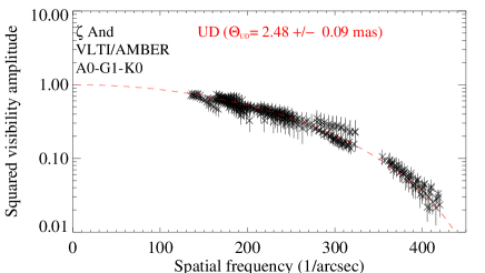
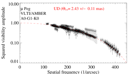
Figure 1: VLTI/AMBER visibility data of $\zeta$ And (top) and of the check star $\mu$ Peg (bottom), compared to uniform disk models.

3.2 Analysis of interferometric data

Table 3: Uniform disk fit results for the VLTI/AMBER data.

Day	FINITO	$\zeta$ And	$\mu$ Peg
14	ON	2.48 $\pm$ 0.06 mas	2.43 $\pm$ 0.07 mas
14	OFF	2.40 $\pm$ 0.21 mas	2.43 $\pm$ 0.06 mas
16	ON	2.53 $\pm$ 0.11 mas	2.42 $\pm$ 0.19 mas
18	ON	2.58 $\pm$ 0.12 mas	2.62 $\pm$ 0.16 mas
$\theta_{\mathrm{UD}}$	all data	2.48 $\pm$ 0.09 mas	2.43 $\pm$ 0.11 mas
$\theta_{\mathrm{LD}}$	all data	2.55 $\pm$ 0.09 mas	2.49 $\pm$ 0.11 mas

Figure 1 shows the resulting visibility data of $\zeta$ And and of the check star $\mu$ Peg obtained from all three observing nights and compared to models of a uniform disk (UD). Because of the relative large errors in the observations, no differences were seen in the measurements from different baselines. Thus all the baselines were used together in the analysis. Table 3 lists the resulting uniform disk diameters of $\zeta$ And and $\mu$ Peg for each of the nights separately, as well as for all three observing nights. When using the data from all the nights together, the diameter is estimated from the data obtained during the nights starting on September 14 and 16, but the error is from all the data, i.e., including the data from the night starting on September 18. This is done because the data quality is significantly lower on the night starting on September 18 than during the two other observing nights.

During the night of September 14, we obtained data with and without the use of the fringe tracker FINITO. The results for these two data sets agree well within the errors for both targets, and we do not see any systematic calibration effects that are caused by the use of FINITO. Deviations between observed visibility values and the UD model are mostly caused by residuals of the compensation of the chromatic piston effect, which was most noticeable on the baseline A0-G1, and by systematic calibration uncertainties due to varying atmospheric conditions. Within the obtained errors of the UD diameter of about 4%, we do not see indications of any elliptical intensity distribution of $\zeta$ And. However, the ellipticity of $\sim$4% expected for the night of September 18 is consistent with our data.

Correction factors between UD diameter and limb-darkened (LD) disk diameters were computed using ATLAS 9 model atmospheres (Kurucz kurucz (1993)). For the spectral types of our target stars $\zeta$ And and $\mu$ Peg and the wavelength range used for our observations, we obtain values for $\theta_{\mathrm{UD}}/\theta_{\mathrm{LD}}$ of 0.974 and 0.976, respectively. The resulting LD diameters are $\theta_{\mathrm{LD}}=2.55\pm 0.09$ mas and $\theta_{\mathrm{LD}}=2.49\pm 0.11$ mas, respectively. Cohen et al. (cohen (1999)) give a diameter of $2.72\pm 0.036$ mas for $\zeta$ And, based on spectro-photometry. This diameter is significantly larger, but the error smaller, than what was obtained in this work. Still, the spectro-photometric observations could be affected by the significant magnetic activity exhibited by $\zeta$ And. The LD diameter of $\mu$ Peg obtained here is consistent with the earlier interferometric measurements of $\theta_{\mathrm{LD}}=2.53\pm 0.09$ mas obtained with the NPOI and $\theta_{\mathrm{LD}}=2.49\pm 0.04$ mas obtained with the Mark III interferometers (Nordgren et al. nordgren (2001) and Mozurkewich et al. mozurkewich (2003)), increasing the confidence in the results presented here.

4 Fundamental parameters

4.1 Radius

The limb darkened diameter of $\zeta$ And, obtained from the interferometric observations, is $2.55\pm 0.09$ mas. Together with the Hipparcos parallax of $17.24\pm 0.26$ mas (van Leeuwen hip (2007)) this can be used to determine the stellar radius with the following formula: $R=\Theta_{\rm LD}\frac{C}{2\pi_{\rm p}}$, where $\Theta_{\rm LD}$ is the limb-darkened angular diameter in radians, $\pi_{\rm p}$ the parallax in arcseconds, and $C$ the conversion from parsecs to meters. For $\zeta$ And this gives stellar radius of $R=15.9\pm 0.8{\rm R}_{\odot}$, which is consistent with the 16.0 R_⊙ estimated in Paper 1.

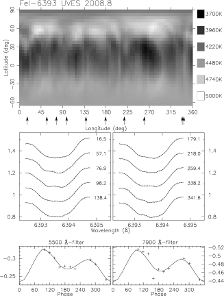
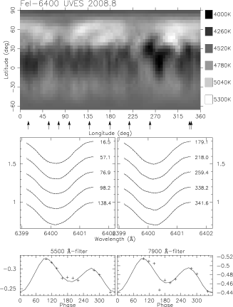
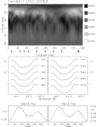
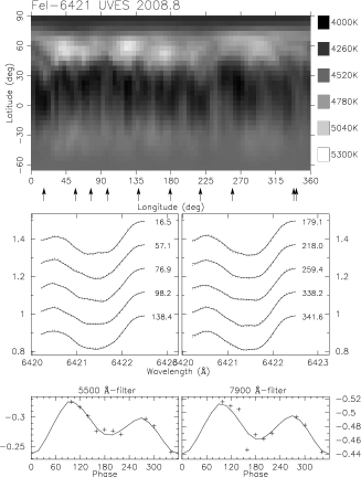
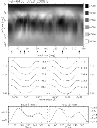
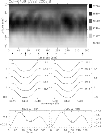
Figure 2: Doppler imaging results of $\zeta$ And obtained with the TempMap_ϵ code. In each plot the temperature map for an individual spectral line is shown with the observed spectra and photometry, including the corresponding fits to the data. In the middle panels, under the continuous line fits, the tiny vertical dashes are the 1-$\sigma$ error bars of the spectroscopic observations.

4.2 Effective temperature

The effective temperature of a star can be calculated from the interferometric diameter determination when combined with a bolometric flux measurement using the formula

$$T_{\rm eff}=\left(\frac{4f_{\rm bol}}{\sigma\Theta_{\rm LD}^{2}}\right)^{1/4},$$ (1)

where $f_{\rm bol}$ is the bolometric flux and $\sigma$ is the Stefan-Boltzmann constant.

The bolometric flux of $\zeta$ And was estimated using measurements on all the available photometric passbands and the getCal tool of the NASA Exoplanet Science Institute’s interferometric observation planning tool suite. The bolometric flux of $f_{\rm bol}=9.863\pm 0.54\times 10^{-10}$ W/m² was obtained. Inserting this value to Eq. 1, together with the limb-darkened angular diameter, gives $T_{\rm eff}$ of $4665\pm 140$ K. This value is very close to, and the same within errors, as the $T_{\rm eff}\approx 4600$ K used for Doppler imaging in Paper 1 and the current work.

5 Doppler imaging

For Doppler imaging we used the code TempMap, which was originally written by Rice et al. (rice89 (1989)). The code performs a full LTE spectrum synthesis by solving the equation of transfer through a set of ATLAS-9 (Kurucz kurucz (1993)) model atmospheres at all aspect angles and for a given set of chemical abundances. Simultaneous inversions of the spectral lines, as well as of the two photometric bandpasses, are then carried out using a maximum-entropy regularization. For the non-spherical $\zeta$ And, a new version of the code was applied: TempMap_ϵ (see Paper 1 and the references therein) takes the distorted geometry of the evolved component in a close binary into account through the distortion parameter $\epsilon$. The elliptical distortion is approximated by a rotation ellipsoid, elongated towards the secondary star: $\epsilon=\sqrt{1-\left(\frac{b}{a}\right)^{2}}$ where $a$ and $b$ are the long and the short axes of the ellipsoid, respectively. The appropriate value of $\epsilon$ for $\zeta$ And, 0.27, as well as the overall system and stellar parameters, were adopted from Paper 1 (Table 2 therein).

The 30 available UVES spectra (three exposures per night) covered 18 days, i.e., one full rotation cycle, thus allowing one Doppler reconstruction. The three nightly observations were averaged, since they were taken within approximately 120 sec. Thus, for further investigation we used the ten averaged spectra with an enhanced S/N value of $\sim$600 or more (see Table 2 for more details on observations).

Doppler imaging was performed for the well-known mapping lines within the 6392–6440 Å spectral range. Doppler maps for Fe i 6393, 6400, 6411, 6421, 6430, and Ca i 6439 are shown in Fig 2. The individual maps revealed similar spot distributions, i.e., mainly cool spots at low latitudes with temperature contrasts of 600–900 K with respect to the unspotted surface of 4600 K. Cool polar features are also recovered, however, with significantly weaker contrast ranging from $\sim$100 K (Fe i 6400) to a maximum of $\sim$700 K (cf. the Fe i 6430 map). Numerous bright features also appear in the iron maps; however, as they occur near dominant cool spots they can be artifacts, so-called “rebound” features (see, e.g., Rice rice (2002)).

Despite the small difference between the temperature contrasts of the respective maps and the spurious bright features, the resulting six Doppler maps are in very good agreement. This similarity is more conspicuous in Fig 3, where the average of the six individual maps is plotted. Averaging did not blur the overall structure. The most prominent feature is the belt of cool spots at the equatorial region, with the strongest concentration of spots located at the phase $\phi=$0.75 and at another cool region ranging between phases $\phi=0.0-0.4$. Also a weak polar feature can be detected. This result is reminiscent of the result in Paper 1, where low-latitude dominant features also tended to concentrate at quadrature positions of opposite hemispheres for both observing seasons.

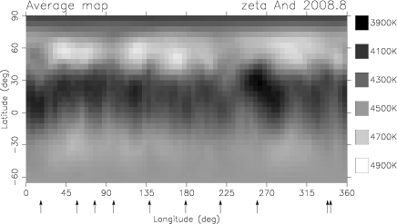
Figure 3: Average map produced from all the maps shown in Fig. 2.

6 Discussion

6.1 Comparison between spherical and ellipsoidal surface geometry in the inversion

Another Doppler imaging code, INVERS7PD, which was written by N. Piskunov (see, e.g., Piskunov et al. pisk90 (1990)) and modified by T. Hackman (Hackman et al. hack (2001)), was also used to obtain a temperature map of $\zeta$ And. In this inversion spherical geometry and only the Fe i 6400 Å line were used. The observations are compared to a grid of local line profiles calculated with the SPECTRUM spectral synthesis code (Gray & Corbally SPECTRUM (1994)) and Kurucz model atmospheres (Kurucz kurucz (1993)). In the calculations, 10 limb angles and nine temperatures between 3500 K and 5500 K were used. Photometry was not used as a constraint in this inversion as the ellipticity effect seen in the light curves cannot be properly taken into account when using spherical geometry.

The result of this inversion is shown in Fig. 4. The main spot structures and the temperature range are similar to the ones in the map obtained with TempMap_ϵ from the Fe i 6400 Å line. The cool spots concentrate on the equatorial region and especially on the quadrature points. The main spot is seen at the phase $\phi$=0.75 in the equatorial region, and there is also a prominent spot at the phase $\phi$=0.25 at higher latitudes. This is missing from the map obtained using TempMap_ϵ, so it is most likely an artifact caused by using spherical geometry on an ellipsoidal star (cf. Fig.3 in Paper 1). Furthermore, at the phase $\phi$=0.25, the equatorial region has a temperature close to that of the unspotted surface, unlike in the map obtained using ellipsoidal geometry. Also, the whole temperature scale is shifted by 100 K towards the cooler temperatures. On the whole, the temperature map obtained with the spherical geometry is very similar to the one obtained using ellipsoidal geometry and TempMap_ϵ. As expected, the main differences occur at the quadrature points and especially at the phase $\phi$=0.25. Also, one has to keep in mind that the tests with TempMap_ϵ show that neglecting the ellipticity in the Doppler imaging reconstruction yields $\sim$50–240% higher $\chi^{2}$ values in comparison to using the correct surface geometry.

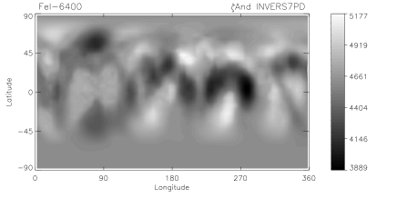
Figure 4: Temperature map of $\zeta$ And obtained with INVERS7PD inversion code using spherical geometry and Fe i 6400 Å line.

Figure 5: Observed $V$ magnitude of $\zeta$ And (crosses) compared to the one calculated from the temperature map obtained using INVERS7PD (line).

The main differences between the results from the spherical and ellipsoidal codes can be seen in the photometry. Figure 5 shows the normalised $V$ observations of $\zeta$ And compared to the ones calculated from the temperature map obtained with the code using spherical geometry. Only around the phases 0.4–0.6 the two light curves show similar behaviour, and the photometry calculated from the INVERS7PD temperature map shows completely different behaviour than the observed one especially around the quadrature points.

6.2 Chromospheric activity

Chromospheric activity of $\zeta$ And was investigated using the H$\alpha$ line profiles, which appeared in absorption during the observations, similarly to the other Balmer lines. Variations in the H$\alpha$ line through the rotation cycle are shown in Fig. 6a. Both the red and the blue wings show strong variation at one, but different, phase. Also, most line profiles clearly show variable behaviour between velocities -100 km/s and +100 km/s. These variations are clearly seen already in the spectra, which have not been corrected to the continuum level. All the spectra show identical continuum shapes, except approximately $\pm$5Å from the H$\alpha$ line, corresponding to the variation also seen in the normalised spectra used in the following analysis.

Figure 6: Variations in the H$\alpha$ profiles of $\zeta$ And. a) The continuum normalised H$\alpha$ profiles. b) Residual profiles after the mean profile has been subtracted. The x-axis gives the velocity in comparison to the mass centre of the giant component.

To investigate the line-profile variations in more detail, the average profile was subtracted from all the profiles, thus creating the residual profiles shown in Fig. 6b. The temporal variations are clearly seen in these profiles. The most prominent features are the two strong absorption features seen at the velocities -350 – 0 km/s and 0 – 100 km/s. A dynamic spectrum, shown in Fig. 7, was also created from the difference profiles. Brighter colours in the plot correspond to enhanced emission and the darker colours to the enhanced absorption. The heliocentric Julian dates of the observations are shown with crosses in the plot. The data for the times where there are no observations are interpolations between the closest timepoints with data. The plotting over the heliocentric Julian date instead of the rotational phase was chosen, as some events are short lived, and the observations in any case cover only slightly more than one rotation. The observational phases are given on the left side of the plot.

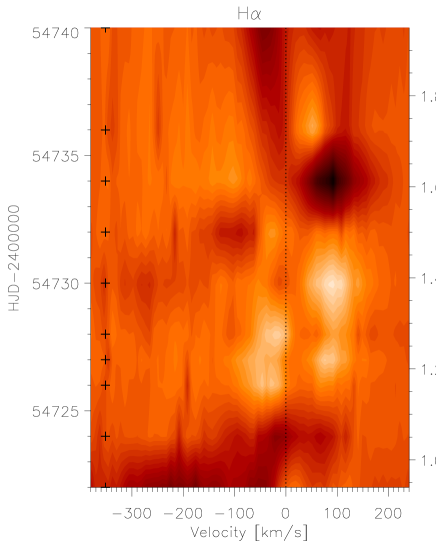
Figure 7: Dynamic spectrum of the H$\alpha$ line based on the residual profiles after the subtraction of the average line profile from the individual profiles. The x-axis gives the velocity and the y-axis the heliocentric Julian date on the left and phase on the right side. The crosses on the lefthand side of the plot give the heliocentric Julian dates of the observations and the dotted line the zero velocity. The brighter the colour, the more emission is observed.

The most noticeable feature in the dynamical spectrum is the strong enhanced absorption around the phase 1.6 at the velocity +100 km/s. If the velocity seen in this absorption system was caused by the stellar rotation, it would be outside the stellar disk and would not be seen in absorption. Thus it must be a cloud of cool gas in the stellar atmosphere that is falling into the star. This could be the final stages of a flare event. No evidence of such an event is seen in the earlier observations, but it could have occurred during the one-night gap in the observations. More enhanced absorption is seen at the first observation (phase 0.94) extending to the very blue, to -300 km/s and beyond. This could be caused by a mass ejection event with a strong line of sight component. In the following observation, more enhanced absorption is seen spanning the velocities -100 – +100 km/s.

Enhanced emission occurs at three main locations: around the phases 1.15–1.30 at the velocities -40 – -70 km/s, around the phases 1.2–1.4 at the velocities +60 – 100 km/s and at the phases 1.7–1.8 at the velocities +40 – 70 km/s. These features have velocities that place them slightly outside the stellar disk, and thus they could be caused by prominences seen at the stellar limb. The prominence seen at the blue edge around phases 1.1–1.3 is most likely the same one as seen at the red edge 0.5 in a later phase (i.e., at phases 1.7–1.8). Also, a weak enhanced absorption feature is seen at phase 1.4 around the velocity -20 km/s, which could be caused by the prominence starting to cross the stellar disk. This prominence could be centred around phase 1.5, which in the binary reference frame is the phase pointing away from the secondary. The enhanced emission seen in the red around phases 1.2–1.4 are, based on their velocities, also most likely caused by prominences. However, they have to be short lived in nature, as no evidence of them is seen in the observations before or after. These prominences would be at the disk centre approximately at phases 1.0 and 1.1, which places them on the side phasing the secondary. They also coincide with the weaker cool region seen around the phases 0.0–0.4 in the Doppler image.

6.3 Long-term magnetic activity of $\zeta$ And

The long-term activity in $\zeta$ And is investigated based on the photometric $V$ and $y$ band observations obtained with the Wolfgang and Amadeus automatic photometric telescopes. The observations between December 1996 and October 2002 were already used in Paper 1. Here, we also use observations obtained between June 27, 2003 and October 25, 2008, in total 211 new $V$ magnitudes.

When all the instrumental differential magnitudes are plotted against the phase, see plot Fig. 8, the variation caused by the ellipticity effect is clearly seen. Still, the observations show much larger scatter around the ellipticity curve than is expected from the measurement error of 0.01–0.02 magnitudes. This indicates that there are also significant variations due to starspots. Evidence of changes in the activity level are also seen when all the observations are plotted against the Julian Date in Fig. 9. In this plot the small crosses give the individual observations and the large crosses the mean of that time period. No mean is given for some time periods, as there are so few measurements, or they are grouped such, that the full light-curve was not sampled.

Figure 8: All the differential $V$ and $y$ magnitudes of $\zeta$ And in the instrumental system plotted against the rotational phase.

Figure 9: All the differential $V$ and $y$ magnitudes plotted against the heliocentric Julian date. The large crosses show the mean magnitudes for that time.

Changes in the mean magnitudes could be interpreted as a solar-like activity cycle. A spectral analysis of the mean measurements was carried out using the Lomb method (Press et al. press (1992)). The result indicates a presence of a cycle with a cycle length of $5.9\pm 0.7$ years, but the false alarm probability is 0.36. Thus the period can be spurious, and more measurements are needed for confirming it.

As can be seen from Fig. 9, $\zeta$ And is on average brighter by 0.014 magnitudes during the VLT observations presented here than during the December 1997 – January 1998 KPNO observations presented in Paper 1. This implies that the spot coverage, and/or the spot temperature, is different between the two epochs. For studying this further, the temperature maps obtained with the Ca i 6439 Å line, were investigated both from the VLT and KPNO observations. The hottest temperature is basically the same in both maps, 4600 K for VLT and 4620 K for KPNO. Still, the coolest temperatures are very different. For the VLT observations, the coolest spots are 3710 K and for the KNPO map 3480 K. Also, the number of surface elements having a temperature of 4000 K or less in the map obtained from the VLT is 75% of the surface elements with those temperatures in the KPNO map. This investigation supports the existence of a activity cycle, which is also indicated by the long-term photometry of $\zeta$ And. Still, one must keep in mind that the temperatures in the Doppler images are very sensitive to the data quality, and the VLT data are superior to the KPNO ones.

7 Conclusions

The following conclusions can be drawn from the optical interferometry, high-resolution spectroscopy and broad band photometry presented in this work.

1. Optical interferometry gives an apparent diameter of $2.55\pm 0.09$ mas for $\zeta$ And. Using the Hipparcos parallax, this translates into a stellar radius of $R=15.9\pm 0.8{\rm R}_{\odot}$, which is in line with the earlier radius determinations.

2. Combining the interferometrically determined diameter and bolometric flux gives an effective temperature of $T_{\rm eff}=4665\pm 140$, which is consistent with the values determined through Doppler imaging.

3. The expected ellipsoidal stellar geometry with $\sim$4% difference between the long and short axes cannot be confirmed with the current interferometric observations, which have errors of about 4% in the diameter measurement. However, the highest ellipticity expected for the night of September 18 is consistent with the data.

4. The Doppler images reveal cool spots on the surface of the primary of the $\zeta$ And binary. The spots are located in the equatorial region, and the main concentration of spots is seen around phase 0.75, i.e., 0.25 in phase from the secondary. Another weaker cool region spans the phases 0.0–0.4, again around the equator. There are also indications of a cool polar cap. On the whole, this spot configuration is very similar to the one seen in the earlier published 1997/1998 data.

5. Long-term photometric observations indicate an activity cycle, but more measurements are needed to confirm this and its period. The investigation of the Doppler maps obtained January 1998 and September 2008 also hint at an activity cycle.

6. The chromospheric activity, investigated from the H$\alpha$-line, shows evidence of both prominences and cool clouds. The prominences do not seem to show any strong evidence of occurring at certain locations in the binary reference frame, nor are they associated with the coolest spot seen on the surface. On the other hand, one of the detected prominences seems to be related to the group of weaker cool spots located at phases 0.0–0.4.

- (1) Bordé, P., Coudé du Foresto, V., Chagnon, G., Perrin, G. 2002, A&A, 393, 183
- (2) Campbell, W. W. 1911, Lick Obs. Bull., 6, No. 199, 140
- (3) Cannon, J. B. 1915, Publ. Dominion Obs. Ottawa, II, No. 6, 141
- (4) Cohen, M.; Walker, R.G., Carter, B., et al. 1999, AJ, 117, 1864
- (5) Dekker, H., D’Odorico, S., Kaufer, A., Delabre, B.,& Kotzlowski, H., 2000, SPIE, 4008, 534
- (6) Glindemann, A., Algomedo, J., Amestica, R., et al. 2003, Proc. SPIE, 4838, 89
- (7) Gray, R.O.,& Corbally, C.J. 1994, AJ, 107, 742
- (8) Granzer, T., Reegen, P.,& Strassmeier, K. G., 2001, AN, 322, 325
- (9) Hackman, T., Jetsu, L.,& Tuominen, I. 2001, A&A, 374, 171
- (10) Hussain, G.A.J. 2002, AN, 323, 349
- (11) Kovári Zs., Bartus, J., Strassmeier K.G., et al., A&A 463, 1071 (Paper 1)
- (12) Kurucz, R.L., 1993, Kurucz CD No. 13
- (13) Le Bouquin, J.-B., Abuter, R., Bauvir, B. et al. 2008, Proc. SPIE, 7013, 701318
- (14) Le Bouquin, J.-B., Absil, O., Benisty, M., et al. 2009, A&A, 498, L41
- (15) Mérand, A., Bordé, P., & Coudé Du Foresto, V. 2006, A&A, 447, 783
- (16) Millour, F., Valat, B., Petrov, R. G., & Vannier, M. 2008, Proc. SPIE, 7013, 701349
- (17) Mozurkewich, D., Armstrong, J.T., Hindsley, R.B., et al. 2003, AJ, 126, 2502
- (18) Nordgren, T.E., Sudol, J.J.,& Mozurkewich, D. 2001, AJ, 122, 2707
- (19) Oláh, K., Kolláth, Z., Granzer, T., et al. 2009, A&A, 501, 703
- (20) Petrov, R.G., Malbet, F., Weigelt, G., et al., 2007, A&A, 464, 1
- (21) Piskunov, N.E., Tuominen, I.,& Vilhu, O. A&A, 230, 363
- (22) Press, W.H., Teukolsky, S.A., Vetterling, W.T. & Flannery, B.P. 1992 in Numerical Recipes in FORTRAN - The Art of Scientific Computing, Second Edition, p. 569–573, Cambridge University Press, New York, USA
- (23) Rice, J.B. 2002, AN, 323, 220
- (24) Rice, J.B., Wehlau, W.H.,& Khokhlova, V.L. 1989, A&A, 208, 179
- (25) Rice, J.B.,& Strassmeier K.G., 1996, A&A, 316, 164
- (26) Rüdiger G., Elstner, D.,& Ossendrijver, M. 2003, A&A 406, 15
- (27) Strassmeier, K.G. 1999, A&A, 347, 225
- (28) Strassmeier, K.G., Hall, D.S., Fekel, F.C.,& Scheck, M. 1993, A&AS, 100, 173
- (29) Strassmeier, K. G., Bartus, J., Cutispoto, G.,& Rodonò, M., 1997, A&AS, 125, 11
- (30) Tatulli, E., Millour, F., Chelli, A., et al. 2007, A&A, 464, 29
- (31) van Leeuwen, F. 2007, A&A, 474, 653
- (32) Wittkowski, M., Boboltz, D.A., Driebe, T., et al. 2008, A&A, 479, L21