The Quasar Accretion Disk Size – Black Hole Mass Relation

Abstract

We use the microlensing variability observed for eleven gravitationally lensed quasars to show that the accretion disk size at a rest-frame wavelength of 2500Å is related to the black hole mass by $\log(R_{2500}/$cm$)=(15.78\pm 0.12)+(0.80\pm 0.17)\log(M_{BH}/10^{9}$M${}_{\sun})$. This scaling is consistent with the expectation from thin disk theory ($R\propto M_{BH}^{2/3}$), but when interpreted in terms of the standard thin disk model ($T\propto R^{-3/4}$), it implies that black holes radiate with very low efficiency, $\log(\eta)=-1.77\pm 0.29+\log(L/L_{E})$ where $\eta=L/(\dot{M}c^{2})$. Only by making the maximum reasonable shifts in the average inclination, Eddington factors and black hole masses can we raise the efficiency estimate to be marginally consistent with typical efficiency estimates ($\eta\approx 10\%$). With one exception, these sizes are larger by a factor of $\sim 4$ than the size needed to produce the observed $0.8\,$µm quasar flux by thermal radiation from a thin disk with the same $T\propto R^{-3/4}$ temperature profile. While scattering a significant fraction of the disk emission on large scales or including a large fraction of contaminating line emission can reduce the size discrepancy, resolving it also appears to require that accretion disks have flatter temperature/surface brightness profiles.

1 Introduction

Despite nearly 40 years of work on accretion disk physics, the simple Shakura & Sunyaev (1973) thin disk model, its relativistic cousins (e.g. Page & Thorne, 1974; Hubeny & Hubeny, 1997; Hubeny et al., 2001; Li et al., 2005) and more sophisticated implementations (e.g. Narayan, Barret & McClintock, 1997; De Villiers, Hawley & Krolik, 2003; Blaes, 2007) remain the standard model despite some observational reservations (see Francis et al., 1991; Koratkar & Blaes, 1999; Collin et al., 2002). Quasar accretion disks cannot be spatially resolved with ordinary telescopes, so we have been forced to test accretion physics through time variability (e.g. Vanden Berk et al., 2004; Sergeev et al., 2005; Cackett, Horne & Winkler, 2007) and spectral modeling (e.g. Sun & Malkan, 1989; Collin et al., 2002; Bonning et al., 2007). One notable success is the use of reverberation mapping (e.g. Peterson et al., 2004) of quasar broad line emission to calibrate the relation between emission line widths and black hole masses. The line emission, though, comes from scales much larger than the accretion disk, and attempts to use similar methods on the continuum emission have had limited success, largely because quasars show little optical variability on the disk light-crossing timescale (Collin et al., 2002; Sergeev et al., 2005).

Gravitational telescopes do, however, provide the necessary resolution to study the structure of the quasar continuum source. Each gravitationally lensed quasar image is observed through a magnifying screen created by the stars in the lens galaxy. Sources that are smaller than the Einstein radius of the stars, typically $\sim 10^{16}$ cm, show time variable fluxes whose amplitude is determined by the source size (see the review by Wambsganss, 2006). Smaller sources have larger variability amplitudes than larger sources. In this paper, we exploit the optical microlensing variability observed in eleven gravitationally lensed quasar systems to measure the size of their accretion disks, and we find that disk sizes are strongly correlated with the masses of their central black holes.

In §2 we describe the monitoring data, the lens models we use based on Hubble Space Telescope ($HST$) images of each system and our microlensing analysis method. In §3 we describe our accretion disk model and our results for the relationship between disk size and black hole mass. While we analyze and discuss the results in terms of a simplified thin disk model, they can be compared to any other model by comparing our measurement of the half light radius to that expected from the model of choice because Mortonson et al. (2005) demonstrate that the half-light radius measured from microlensing is essentially independent of the assumed disk surface brightness profile. The surface brightness profile is best probed by measuring the dependence of the microlensing amplitude on wavelength (see Anguita et al., 2008; Poindexter et al., 2008; Agol et al., 2009; Bate et al., 2008; Floyd et al., 2009; Mosquera et al., 2009). In §4, we discuss the results and their implications for thin accretion disk theory. All calculations in this paper assume a flat $\Lambda$CDM cosmology with $h=0.7$, $\Omega_{M}=0.3$ and $\Omega_{\Lambda}=0.7$.

2 Data and Analysis

We collected new monitoring data in the systems HE 0435–1223, FBQ 0951+2635, HE 1104–1805, SDSS 1138+0314, SBS 1520+530 and Q 2237+030 in the $r$-, $R$- and $V$-bands on the SMARTS 1.3m using the ANDICAM optical/infrared camera (DePoy et al., 2003), the Wisconsin-Yale-Indiana (WIYN) observatory using the WIYN Tip–Tilt Module (WTTM), the 2.4m Hiltner telescope at the MDM Observatory using the MDM Eight-K, Echelle and RETROCAM (Morgan et al., 2005) imagers and the 6.5m Magellan Baade telescope using IMACS (Bigelow et al., 1999). We supplemented our monitoring data with published quasar light curves from Paraficz et al. (2006), Schechter et al. (1997), Wyrzykowski et al. (2003), Ofek & Maoz (2003), OGLE (Wozniak et al., 2000a, b), Gaynullina et al. (2005), and Poindexter et al. (2007). We measured the flux of each image by comparison to the flux from reference stars in the field of each lens. Our analysis of the monitoring data is described in detail by Kochanek et al. (2006). In systems with published time delays, we offset the light curves by the delays to eliminate the intrinsic source variability. In this paper we also make use of previously reported optical accretion disk sizes for the lensed quasars QJ 0158–4325 (Morgan et al., 2008a), SDSS 0924+0219 (Morgan et al., 2006), SDSS 1004+4112 (Fohlmeister et al., 2008), PG 1115+080 (Morgan et al., 2008a) and RXJ 1131$-$1231 (Dai et al., 2010). SDSS 0924+0219, SDSS 1138+0314 and Q 2237+030 do not have published time delays but are all quadruply lensed quasars with short ($\lesssim 15$ days) estimated delays. Since the typical timescale for microlensing is significantly longer than this ($\gtrsim 1$ year), we ignored the delays in these systems and used their raw lightcurves in our microlensing analysis. For QJ 0158–4325 we developed an analysis method that allowed us the simultaneously estimate the time delays and disk sizes including their mutual uncertainties, the details of which are described in Morgan et al. (2008a).

All eleven lenses have been observed in the $V$- (F555W), $I$- (F814W) and $H$-bands (F160W) using the WFPC2, ACS/WFC and NICMOS instruments on HST. We fit these images as combinations of point sources for the quasars and (generally) de Vaucouleurs models for the lenses as described in Lehár et al. (2000). These provided the astrometry used for lens models and defined a constant mass-to-light ($M/L$) ratio model for the mass distribution in the lens models. We modeled each system using the GRAVLENS software package (Keeton, 2001). For all systems except the cluster lens SDSS 1004+4112, we generate a series of ten models starting from a constant $M/L$ model and then adding an NFW (Navarro, Frenk & White, 1996) halo. The sequence is parametrized by $f_{M/L}$, the mass fraction represented by the visible lens galaxy relative to a constant $M/L$ model. In general, we start with the constant $M/L$ model, $f_{M/L}=1$, and then reduce its mass in increments of $\Delta f_{M/L}=0.1$ with the NFW halo’s mass rising to compensate. For the cluster-lensed quasar SDSS 1004+4112, we use the fixed mass model from Fohlmeister et al. (2007), and we assume a set of 10 evenly spaced stellar mass fractions in the range $0.1\leq\kappa_{*}/\kappa\leq 1.0$. Thus, our results marginalize over any uncertainties in the dark matter halos of the lenses. For typical lenses, which we expect to be dark matter dominated, microlensing favors low stellar mass fractions (e.g. Morgan et al., 2008b; Dai et al., 2010; Chartas et al., 2009; Pooley et al., 2009; Mediavilla et al., 2009).   We adopt, however, a very conservative philosophy and include a broad spectrum of models even though a stronger prior favoring dark-matter dominated models is relatively easy to justify. We do this so that our estimates of the source sizes depend as little as possible on other model assumptions.  We have nonetheless tested the sensitivity of the size estimates on lens model dark matter fraction priors, and we have found very weak, if any, dependence.

These lens models provide the convergence $\kappa$, shear $\gamma$ and stellar surface density $\kappa_{*}$ needed to define the microlensing magnification patterns. We assume a lens galaxy stellar mass function $dN(M)/dM\propto M^{-1.3}$ with a dynamic range of a factor of 50 that approximates the Galactic disk mass function of Gould (2000, see also Poindexter & Kochanek 2010a). We also know from previous theoretical studies that the choice of the mass function will have little effect on our conclusions given the other sources of uncertainty (e.g. Paczynski, 1986; Wyithe et al., 2000). For the typical lens we generated 4 magnification patterns for each image in each of the 10 lens models. We gave the magnification patterns an outer scale of $20\langle R_{E}\rangle$, where $\langle R_{E}\rangle$ is the Einstein radius for the mean stellar mass $\langle M\rangle$. This outer dimension is large enough to fairly sample the magnification pattern, while the pixel scale of the 4096² magnification patterns is small enough to resolve the accretion disk. We determined the properties of the accretion disk by modeling the observed light curves using the Bayesian Monte Carlo method of Kochanek (2004) (also see Kochanek et al., 2007). For a given disk model, we randomly generate light curves, fit them to the observations and then use Bayesian methods to compute probability distributions for the disk size averaged over the lens models, the likely velocities of the observer, lens, source, stars and the mean microlens mass $\langle M\rangle$. We used the velocity model from Kochanek (2004), which used the projected CMB dipole (Kogut et al., 1993) for the observer, a stellar velocity dispersion set by the Einstein radius of the lens and peculiar velocity scales for the lens and source of $235/(1+z)$ km s^-1. We use a prior on the mean microlens mass of $0.1{\rm M_{\sun}}<\langle M\rangle<1.0{\rm M_{\sun}}$, but the disk size estimates are insensitive to this assumption (see Kochanek, 2004; Morgan et al., 2008b).

An obstacle to our analysis technique is how to handle differences between the observed flux ratios and the flux ratios of the trial lightcurves. In systems where we are confident that the intrinsic flux ratios are known (e.g. PG 1115+080, for which Chiba et al., 2005, measured mid-IR flux ratios), we set a prior to favor model lightcurves within 0.1 mag of the intrinsic flux ratios. In most cases, however, the intrinsic flux ratios are not known because all observed flux ratios can be affected by chromatic microlensing or dust extinction. In these cases we set a much looser prior on this magnification offset, typically $\sim 0.5$ mag. Loosening the prior on the magnification offset degrades our ability to to estimate the dark matter content of the lens galaxy, but it has little effect on accretion disk size measurements (see Dai et al., 2010, for a detailed demonstration of this effect in RXJ 1131$-$1231).

We use black hole mass estimates for the quasars that are based on observed quasar emission line widths and the locally calibrated virial relations for black hole masses, for which we adopt the combined normalizations of Onken et al. (2004) and Greene & Ho (2007). For most systems we simply used the black hole mass estimates from Peng et al. (2006) based on the C IV ($\lambda 1549$Å), Mg II ($\lambda 2798$Å) and H$\beta$ ($\lambda 4861$Å) mass-linewidth relations. For SDSS 1138+0314, we measured the width of the C IV (1549Å) line in optical spectra from the Sloan Digital Sky Survey (Adelman-McCarthy et al., 2006) and for Q 2237+030 we used the C IV line width measurement from Yee & De Robertis (1991). We estimated the black hole masses for these systems using the virial relation of Vestergaard & Peterson (2006). For SDSS 1004+4112, we measured the width of the Mg II ($\lambda 2798$Å) emission line in spectra from Inada et al. (2003) and Richards et al. (2004) and used the McLure & Jarvis (2002) Mg II virial relation to estimate its black hole mass. These mass estimates are reliable to approximately 0.3 dex (see McLure & Jarvis, 2002; Kollmeier et al., 2006; Vestergaard & Peterson, 2006; Peng et al., 2006).

3 Results

We model the surface brightness profile of the accretion disk as a power law temperature profile, $T\propto R^{-3/4}$, matching the outer regions of a Shakura & Sunyaev (1973) thin disk model. We neglect the central depression of the temperature due to the inner edge of the disk and corrections from general relativity to avoid extra parameters. The effect of this simplification on our size estimates is small compared to our measurement uncertainties provided the disk size we obtain is significantly larger than the radius of the inner disk edge. We will compare three disk size estimates in the context of this simple model. First, there is our size measurement from the microlensing, $R_{S}$. This microlensing size should be viewed as a measurement of the half-light radius, but we parametrize the results in terms of the simple thin disk model in order to facilitate comparisons to the thin disk model. Converted to a half-light radius, $R_{1/2}=2.44R_{S}$, the measurements will be nearly model-independent (see Mortonson et al., 2005). Second, there is the theoretically expected size as a function of black hole mass in the thin disk model (see Eqn. 2 below). Third, there is the thin-disk size which would yield the observed optical flux assuming thermal radiation and a $T\propto R^{-3/4}$ temperature profile (see Eqn. 3 below). We emphasize that while the second and third size estimates are based upon the same accretion disk model, they differ in that they take different measured quantities, either $M_{BH}$ or $I$-band flux, as an argument. Collin et al. (2002) had previously noticed that the theory size (Eqn. 2) and the flux size (Eqn. 3) may be discrepant.  Pooley et al. (2007) argued that the microlensing sizes and the theory sizes (Eqn. 2) are discrepant, but they used black hole masses based largely on estimates of the bolometric luminosity, which in some sense forced a reconciliation of the flux and theory sizes.

We assume that the disk radiates as a black body, so the surface brightness at rest wavelength $\lambda_{rest}$ is

$$f_{\nu}={2h_{p}c\over\lambda_{rest}^{3}}\left[\exp\left({R\over R_{\lambda_{rest}}}\right)^{3/4}-1\right]^{-1}$$ (1)

where the scale length

$$R_{\lambda_{rest}}=\left[{45G\lambda_{rest}^{4}M_{BH}\dot{M}\over 16\pi^{6}h_{p}c^{2}}\right]^{1/3}=9.7\times 10^{15}\left({\lambda_{rest}\over{\rm\micron}}\right)^{4/3}\left({M_{BH}\over 10^{9}{\rm M_{\sun}}}\right)^{2/3}\left({L\over\eta L_{E}}\right)^{1/3}{\rm cm}$$ (2)

is the radius at which the disk temperature matches the wavelength, $kT_{\lambda_{rest}}=h_{p}c/\lambda_{rest}$, $h_{p}$ is the Planck constant, $k$ is the Boltzmann constant, $M_{BH}$ is the black hole mass, $\dot{M}$ is the mass accretion rate, $L/L_{E}$ is the luminosity in units of the Eddington luminosity, and $\eta=L/(\dot{M}c^{2})$ is the accretion efficiency. We can also compute the size under the same model assumptions based on the magnification-corrected $I$-band quasar fluxes measured in HST observations as

$$R_{I}=2.83\times 10^{15}{1\over\sqrt{\cos i}}\left({D_{OS}\over r_{H}}\right)\left({\lambda_{I,obs}\over{\rm\micron}}\right)^{3/2}10^{-0.2(I-19)}\>h^{-1}\>{\rm cm}$$ (3)

where $D_{OS}/r_{H}$ is the angular diameter distance to the quasar in units of the Hubble radius, $I$ is the magnification-corrected magnitude and $i$ is the disk inclination angle.

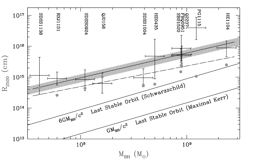
Figure 1: Inclination-corrected accretion disk size $R_{2500}$ versus black hole mass $M_{BH}$. The solid line through the data shows our best power-law fit to the data and the dot-dashed line shows the prediction from thin disk theory ($L/L_{E}=1$ and $\eta=0.1$). The shaded band surrounding the best fit shows the expected variance due to inclination. Disk sizes are corrected to a rest wavelength of $\lambda_{rest}=2500$Å and the black hole masses were estimated using emission line widths. The filled points without error bars are $R_{2500}$ estimates based on the observed, magnification-corrected $I$-band fluxes. They have typical uncertainties of $0.1$-$0.2$ dex. Solid lines at the bottom of the plot show the innermost stable circular orbit for a maximally rotating Kerr black hole and a Schwarzschild black hole, representing a plausible range of radii for the inner edge of an accretion disk.

Our results are shown in Figures 1 through 3 and summarized in Table 1. For the comparison with theory and the figures, we corrected the measured sizes to $\lambda_{rest}=2500{\rm\AA}$ assuming the $\lambda^{4/3}$ scaling of thin disk theory and a mean inclination $\langle\cos i\rangle=1/2$. We chose 2500Å because it was typical of the actual rest-frame wavelength (see Table 1), minimizing the sensitivity of our estimates to any uncertainty in the true wavelength scaling. Only the size of RXJ1131–1231 is strongly affected by changing the scaling of size with wavelength, because of its remarkably low source redshift ($z_{s}=0.658$). However, even if we vary the temperature profile of the disk from $T\propto R^{-1/2}$ (e.g. Francis et al., 1991) to $T\propto R^{-1}$, corresponding to the range from $R_{\lambda}\propto\lambda^{2}$ to $R_{\lambda}\propto\lambda$, the wavelength-corrected disk size changes only by $\sim 25\%$ and the fit parameters for the relationship between disk size and black hole mass change by less than $5\%$.

Although we use a face-on disk model, we need to consider the role of inclination. Both the microlensing size and the flux size (Eqn. 3) are set by the projected area of the disk, so the true microlensing disk scale should be $1/\sqrt{\cos i}$ of the face-on estimate. When we average over an ensemble of systems assuming a random distribution of inclination angles, we are averaging over projected areas $\langle R_{fit}^{2}\rangle=\langle R_{true}^{2}\cos i\rangle=(1/2\pm 1/2\sqrt{3})R_{true}^{2}$, so we correct our measurements to $\langle R_{true}\rangle=\sqrt{2}R_{fit}$. We discuss the consequences of other inclination distributions in § 4. In Table 1 and Figs. 1 and 3, we use this average correction for both the microlensing and flux sizes. The gray band in Fig. 1 shows the expected extra variance of $1/2\sqrt{3}$ arising from the inclination if we view our fits as matching the predicted and observed projected areas.

There are two striking facts illustrated by the figures. First, we clearly see from Fig. 1 that the microlensing sizes are well correlated with the black hole mass. A power-law fit between $R_{2500}$ and $M_{BH}$ including the uncertainties in both quantities yields

$$\log\left({R_{2500}\over{\rm cm}}\right)=(15.78\pm 0.12)+(0.80\pm 0.17)\log\left({M_{BH}\over 10^{9}{\rm M_{\sun}}}\right),$$ (4)

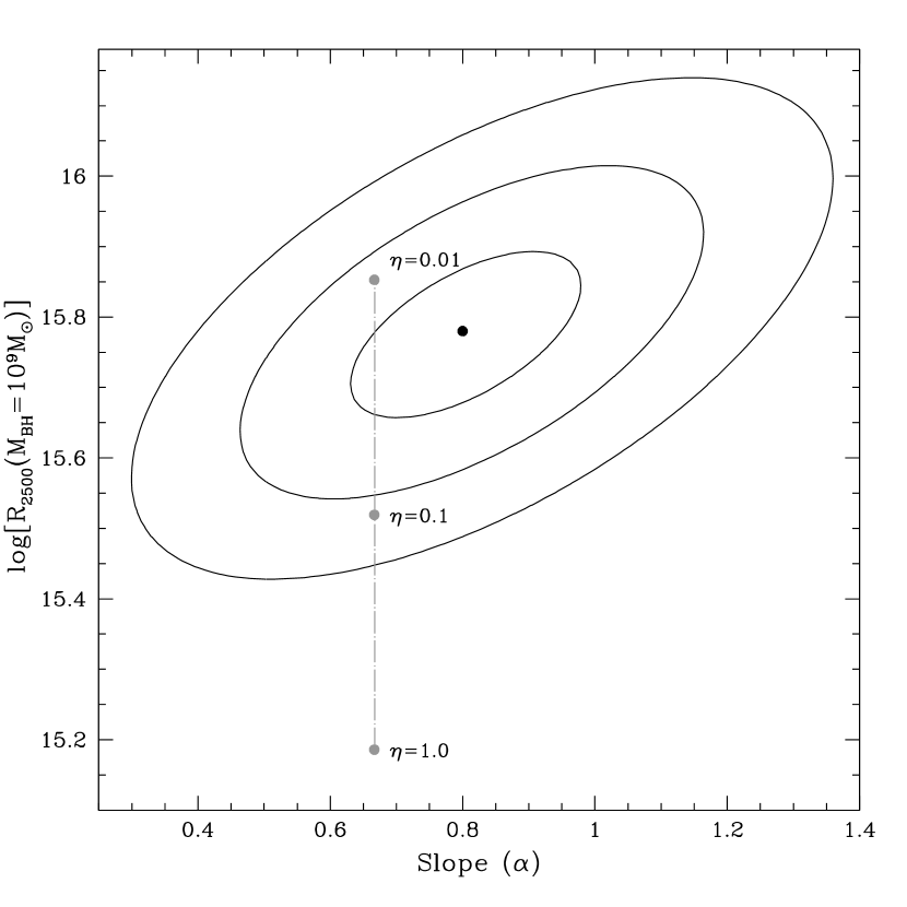
Figure 2: Results of the power-law fit to $R_{2500}$ as a function of black hole mass. The contours show the $1-3\sigma$ one-parameter confidence intervals for the slope $\alpha$ and the normalization $R_{2500}(M_{BH}=10^{9}{\rm M_{\sun}})$ for the 2500Å accretion disk size corresponding to $M_{BH}=10^{9}{\rm M_{\sun}}$. The best-fit value is indicated with a black point. The filled points along the dot-dashed line are theoretical thin disk sizes for quasars radiating at the Eddington limit and with efficiencies of $\eta=L/(\dot{M}c^{2})=0.01$, $0.1$ or $1.0$.

which is consistent with the predicted slope from thin disk theory ($R\propto M_{BH}^{2/3}$). If we fix the slope with mass to 2/3 (see Fig. 2), the relation implies a typical Eddington factor of $\log(L/\eta L_{E})=1.77\pm 0.29$. Kollmeier et al. (2006) estimate that the typical quasar has $L/L_{E}\approx 1/3$, which would indicate a radiative efficiency of $\eta=L/(\dot{M}c^{2})\simeq 0.006$. This efficiency is very low compared to standard models (e.g. Gammie, 1999) and observational constraints on radiative efficiency derived from the local black hole mass and quasar luminosity functions (e.g. Yu & Tremaine, 2002; Soltan, 1982). We discuss this point further in § 4.

The goodness of fit, $\chi^{2}=9.15$ for $9$ degrees of freedom ($\chi^{2}/N_{dof}=1.07$) without including any effects from the spread in inclination, suggests that the errors on the size and $M_{BH}$ estimates are appropriate. While the formal uncertainties in $M_{BH}$ from the line width relations are only $\sim 0.1$ dex, the systematic uncertainties are generally believed to be closer to $0.33$ dex (McLure & Jarvis, 2002; Kollmeier et al., 2006; Vestergaard & Peterson, 2006; Peng et al., 2006). If we fit the relation assuming that this is an additional random error in each black hole mass, then we find $\log\left({R_{2500}/{\rm cm}}\right)=(15.9\pm 0.2)+(1.0\pm 0.3)\log\left({M_{BH}/10^{9}{\rm M_{\sun}}}\right)$ with a goodness of fit $\chi^{2}/N_{dof}=0.59$. This implies either that $0.33$ dex of random uncertainty for each individual black hole mass is too large or that we have over-estimated the uncertainties in the size measurements.

The low efficiency estimate is closely related to the argument by Pooley et al. (2007) that the sizes estimated from microlensing are larger than expected from thin disk theory, but the comparison is not exact because Pooley et al. (2007) used black hole masses determined largely from estimates of the bolometric luminosity rather than the emission line width method.   This causes some covariance between their theory and flux sizes so an exact comparison to our results is difficult. Nonetheless, compared to Pooley et al. (2007) we find a smaller discrepancy because our full calculations of the microlensing sizes tend to be somewhat smaller (by an average of 0.2 dex for our four common systems) than those of Pooley et al. (2007). Despite these differences, our low estimate for the radiative efficiency is essentially the same as the problem pointed out by these authors.

Second, there is a much more striking discrepancy between both the microlensing and theory size estimates (Eqn. 2) with the flux sizes (Eqn. 3).  While most of the offset between the microlensing size measurements and the expectations from thin disk theory could be explained by the existing uncertainties, the offset from the estimate based on the quasar flux is more significant. The measured disk sizes are significantly larger than the flux sizes in all systems except QJ 0158–4325 (see Fig. 3), with an average offset of $0.6\pm 0.3$ dex. Simply put, the quasars are not sufficiently luminous to have the sizes estimated from microlensing while radiating as black bodies with a $T\propto R^{-3/4}$ temperature profile.

4 Discussion

Using microlensing we have made the first observational demonstration of the dependence of accretion disk sizes on black hole mass. While the slope of the relation is still relatively uncertain, it is consistent with the scaling of $M_{BH}^{2/3}$ expected for quasars with similar Eddington ratios. The absolute scales correspond to relatively low radiative efficiencies, which we discuss in detail below.

Like Pooley et al. (2007) we find that the microlensing estimates of the disk size are somewhat larger than would be expected from thin disk theory for typical Eddington ratios ($L/L_{E}\sim 1/3$, e.g. Kollmeier et al. 2006).  We can examine this in terms of our estimate of the radiative efficiency

$$\log\eta=(-2.25\pm 0.29)+\log\left(3{L\over L_{E}}\right)+2\log\left({M_{BH,true}\over M_{BH,est}}\right)+{3\over 2}\log(2\,\langle\cos i\rangle),$$ (5)

where $3L/L_{E}$ is the Eddington ratio normalized to $1/3$, $M_{BH,true}/M_{BH,est}$ is the average ratio of the true black hole masses to our estimates, and $2\langle\cos i\rangle$ is the dependence on changes in the mean inclination angle from that for a uniform distribution. Constraints derived from matching the total radiated energy of quasars to the local black hole mass function (e.g. Soltan, 1982; Yu & Tremaine, 2002) argue for a typical radiative efficiency close to 10% or $\log\eta=-1$ and even higher efficiencies for the most luminous quasars.  It is barely possible to reconcile our estimates with these.  First, in unification models (e.g. Antonucci, 1993; Urry & Padovani, 1995) the inclination angles of optical quasars are preferentially face-on rather than uniformly distributed.  Indeed, the first microlensing measurements of a disk inclination angle favor face-on viewing angles (Poindexter & Kochanek, 2010b).  If, for example, we assumed quasars were uniformly distributed only over the range $1/2<\cos i<1$, then our estimate of the efficiency rises by $0.2$ dex.  The methods used in Kollmeier et al. (2006), or any other study of Eddington factors, will generally be more reliable for the distribution of the Eddington factors than for the absolute values.  The absolute values are sensitive to the absolute calibration of the black hole masses and correctly estimating the bolometric luminosity.  Shifting the typical quasar from $L/L_{E}=1/3$ to $L/L_{E}\simeq 1$ would reduce the discrepancy by $0.5$ dex.  Similarly, most studies of estimating black hole masses from emission line widths would accept that there are absolute calibration uncertainties of order $0.3$ dex in $M_{BH,true}/M_{BH,est}$.  Unfortunately, we gain only this factor rather than its square if we make $M_{BH,true}/M_{BH,est}=3$, despite Eqn. 5, because the estimates of the Eddington factor also have to be adjusted downwards if we raise the estimated black hole mass.  If we move all three of these terms in the same direction ($L/L_{E}=1$ instead of $1/3$, $M_{BH,true}/M_{BH,est}=3$ instead of $1$ and $\langle\cos i\rangle=3/4$ instead of $1/2$) we can we bring $\log\eta=-1.29\pm 0.29$ within $1\sigma$ of 10% efficiency.

This may be stretching the allowed parameter shifts, but it does not address the still larger discrepancies between either the microlensing or the theory sizes with the flux sizes.  To emphasize this point, if we estimate $\eta$ from the flux sizes we find $\log\eta=-0.43\pm 0.21$ which has problems of the opposite sign.  Are these discrepancies between these three size estimates due to a problem in the measurements, an oversimplification of the disk model or a fundamental problem in the thin disk model? We have tested our approach using Monte Carlo simulations of light curves and verified that we recover the input disk sizes. Our results are also only weakly sensitive to the assumed prior on the microlens masses (see Kochanek, 2004; Morgan et al., 2008b, for a discussion). Dai et al. (2010) in their detailed study of microlensing in RXJ 1131$-$1231 show that none of the details of our approach significantly affect the size estimates. This suggests that we must look to significant changes in the physical model to explain the differences. Fig. 4 illustrates the consequences of four possible modifications: scattered light, contaminating emission, effects of the inner disk edge, and changes in the temperature profile. In each case we rescale the ratio of the flux and microlensing sizes while holding the optical flux and the half light radius of the disk fixed to see if we can shift the ratio from the observed $-0.6\pm 0.3$ dex. Holding the half-light radius fixed should mean that the new model will be consistent with the microlensing constraints (Mortonson et al., 2005). We generalize the temperature profile of Eqn. 1 to

$$T(R)\propto\left({R_{\lambda}\over R}\right)^{\beta}\left[1-\left({R_{in}\over R}\right)^{1/2}\right]^{1/4}$$ (6)

with locally thermal emission for $R>R_{in}$. Our fiducial models have $\beta=3/4$ and $R_{in}=0$. Here $R_{\lambda}$ is just a scale length and does not correspond to the expression in Eqn. 2. Because Eqn. 6 is not based on a theoretical model, we have no means of relating $R_{\lambda}$ to physical parameters. We can attempt to reconcile the flux and microlensing sizes with Eqn. 6, but we cannot use it to examine the efficiency problem.

We have assumed so far that the observed optical flux is emission directly from the accretion disk, hence we will overestimate the microlensing size of the disk if an appreciable fraction of the emission originates on scales larger than the accretion disk. For example, if we fit the data modeling 30% of the observed light as unmicrolensed emission from scales much larger than the accretion disk, then we find that the microlensing size estimates shrink by 20-50%. Dai et al. (2010) investigated this problem in detail for RXJ 1131$-$1231. As the fraction of contaminating light increases, the disk has to become more compact in order to produce the same amplitude of microlensing variability. This large scale emission can be either scattered emission from the disk or contaminating emission from some other source. The two effects differ because the flux from the disk is unchanged by scattering, while the flux from the disk is reduced by the amount of contaminating emission.

The main sources of contamination will be emission from the larger and minimally microlensed line emitting regions (e.g. Sluse et al., 2007; Sugai et al., 2007) and the unmicrolensed emission of the quasar host galaxy. Here we need not worry about the host galaxy as we are examining the rest frame ultraviolet emission of luminous quasars. The sources of line contamination include not only the obvious broad/narrow lines but also the broad Fe II and Balmer continuum emission (Maoz et al., 1993; Vestergaard & Peterson, 2005) that can represent $\sim 30\%$ of the apparent continuum flux at some wavelengths (Netzer & Willis, 1983; Grandi, 1982). Table 1 notes the possible sources of broad line contamination for each system. While four of the systems have the Mg II line in the filter band pass, the Balmer continuum and Iron line complexes are probably the dominant source of line contamination. However, the line emission is generally reprocessed harder radiation, so as we increase the line contamination to reduce the microlensing size of the disk, we also reduce the optical flux coming from the disk and hence the flux size of the disk. Thus, producing the large scale emission by scattering the disk emission reduces the microlensing size but leaves the flux size unchanged, while producing it by line contamination reduces both size estimates. Fig. 4 shows that in our simple model, contamination and scattering cannot bring the two sizes into agreement unless most of the emission is not coming directly from the disk. Our discussion of scattering here assumes it is not accompanied by significant changes in the photon energy. If much of the observed optical radiation is due to Compton scattering of softer photons, then the net effect would depend on the physical scale of the scattering medium, particularly since the highest densities of hot electrons are likely to be on similar scales to that of the accretion disk. One consequence of reducing the directly observed emission from the disk is that the fractional variability of the disk emission rises in proportion, as the (re)emission on large (parsec) scales cannot produce the short time scales of the intrinsic quasar variability. This consideration probably rules out models in which a minority of the observed flux comes directly from the disk.

The problem is also not a consequence of the simplifications in the disk model, namely the neglect of the inner edge and the different inner temperature profile of a relativistic disk (e.g. Page & Thorne, 1974). Whether we use the microlensing or flux scales for the disk, the optical emission is mostly radiated far from the scale expected for the inner edges of disk ($\sim 60r_{g}$ rather than a few $r_{g}=GM_{BH}/c^{2}$). Dai et al. (2010) examined this problem for RXJ1131$-$1231 using the full relativistic Hubeny et al. (2001) models and found few changes from our simple standard model. We illustrate this here by adding an inner edge to the disk with $R_{in}=0.1R_{\lambda}$, which is larger than we would expect from the sizes and black hole masses of these sources. As shown in Fig. 4, this has little effect on the size ratio unless the disk temperature profile is very steep.

The final possibility we consider is changing the temperature profile of the disk. As shown in Fig. 4, using a temperature profile flatter than $\beta=3/4$ has the strongest effect on the size ratio of all the changes we consider. A temperature slope closer to $\beta\sim 0.5$ can bring the two scales into agreement. With the addition of a scattered or contaminating component, smaller changes are needed, and the inner disk edge becomes less important for the flatter profiles. Steeper temperature profiles, on the other hand, worsen the problem, although in this regime the inner disk edge also becomes important.

Fig. 4 also shows the existing microlensing limits on $\beta$ from Anguita et al. (2008), Bate et al. (2008), Eigenbrod et al. (2008), Floyd et al. (2009), and Poindexter et al. (2008), based on the wavelength dependence of the microlensing. Mosquera et al. (2009) also report results consistent with $\beta\sim 0.75$. With the exception of Floyd et al. (2009), these initial studies are consistent with both $\beta=3/4$ and the shallower profiles that would help to resolve the differences in the size estimates. The discrepant result of Floyd et al. (2009) requiring a steeper slope is likely a consequence of their approach. Unlike the other studies, both Bate et al. (2008) and Floyd et al. (2009) use only the color differences between images observed at single epochs rather than light curves. This means that at any wavelength they can only set an upper bound on the source size – it is the amplitude observed during caustic crossings that sets the lower bounds, and that can only be measured using time variability. However, given only a set of upper limits on the sizes that are smaller for shorter wavelengths, the estimate for $\beta$ will be determined by the priors used for the source sizes. In particular, the linear priors used by Bate et al. (2008) and Floyd et al. (2009) will favor steep temperature profiles, while a logarithmic prior would favor shallow temperature profiles. The same problem occurs for sparsely sampled light curves, as illustrated by the studies of X-ray microlensing by Morgan et al. (2008b) and Dai et al. (2010), where the lower limits to the X-ray size are found to be prior-dependent. From this point of view Bate et al. (2008) and Floyd et al. (2009) are really upper bounds on $\beta$, and analyses of light curves will be required to determine a lower bound.

Arguments for a flatter emissivity profile in accretion disks have existed for a long time, largely based on the mismatch between the predicted and observed spectra of quasars (see the reviews by Koratkar & Blaes (1999) and Blaes (2004)). The emission profile can be flattened either by raising the temperature of the outer disk (e.g. irradiation of the outer disk by the inner) or by changing the balance between radiation and advection in the inner disk (e.g. thick or slim disks). Microlensing provides the first probe able to actually measure the physical scales associated with the emission regions, and the results are clearly beginning to test the simplest theories. As the numbers of systems, the uncertainties in the size measurements and the wavelength range spanned by the measurements increases, microlensing can quantitatively address all these issues.

Table 1: Measured and Derived Quantities

Object	Line	FWHM	$M_{BH}$	$\log(R_{S}/{\rm cm})$	$\lambda_{rest}$	BLR	$I_{corr}$	$\log(R_{S}/{\rm cm})$
		Å (observed)	$(10^{9}~{}{\rm M_{\sun}})$	(microlensing)	(µm)	Contaminant	(mag)	(thin disk flux)
QJ0158–4325	Mg ii	40	0.16	$14.9_{-0.3}^{+0.3}$	0.306	Balmer, Fe ii UV, Mg ii	$19.09\pm 0.12$	$15.2\pm 0.1$
HE0435–1223	C iv	70	0.50	$15.7_{-0.7}^{+0.5}$	0.260	Balmer, Fe ii UV	$20.76\pm 0.25$	$14.9\pm 0.1$
SDSS0924+0219	Mg ii	61	0.11	$15.0_{-0.4}^{+0.3}$	0.277	Balmer, Fe ii UV, Mg ii	$21.24\pm 0.25$	$14.8\pm 0.1$
FBQ0951+2635	Mg ii	70	0.89	$16.1_{-0.4}^{+0.4}$	0.313	Balmer, Fe ii UV, Mg ii	$17.16\pm 0.11$	$15.6\pm 0.1$
SDSS1004+4112	Mg ii	134	0.39	$14.9_{-0.3}^{+0.3}$	0.228	Balmer, Fe ii UV	$20.97\pm 0.44$	$14.9\pm 0.2$
HE1104-1805	C iv	103	2.37	$15.9_{-0.3}^{+0.2}$	0.211	Balmer, Fe ii UV	$18.17\pm 0.31$	$15.4\pm 0.1$
PG1115+080	Mg ii	127	1.23	$16.6_{-0.4}^{+0.3}$	0.257	Balmer, Fe ii UV	$19.52\pm 0.27$	$15.1\pm 0.1$
RXJ1131–1231	H$\beta$	90	0.06	$15.3_{-0.2}^{+0.2}$	0.422	Balmer, Fe ii Optical	$20.73\pm 0.11$	$14.8\pm 0.1$
SDSS1138+0314	C iv	25	0.04	$14.9_{-0.6}^{+0.6}$	0.203	Balmer, Fe ii UV	$21.97\pm 0.19$	$14.6\pm 0.1$
SBS1520+530	C iv	75	0.88	$15.7_{-0.2}^{+0.2}$	0.245	Balmer, Fe ii UV	$18.92\pm 0.13$	$15.3\pm 0.1$
Q2237+030	C iv	48	0.9	$15.6_{-0.3}^{+0.3}$	0.208	Balmer	$17.90\pm 0.44$	$15.5\pm 0.2$

Note. — $R_{S}$ from microlensing is the accretion disk size at $\lambda_{rest}$, the rest-frame wavelength corresponding to the center of the monitoring filter used for that quasar’s light curve. Use half-light radii ($R_{1/2}=2.44R_{S}$) to compare these size measurements to other disk models. Significant sources of unmicrolensed flux from the QSO Broad Line Region (BLR) that fall into or overlap with the observing pass band are indicated: Balmer Continuum ($\lambda\lesssim 3650$Å), Fe ii UV Continuum ($\lambda\lesssim 3100$Å), Fe ii Optical Continuum ($4240$Å $\lesssim\lambda\lesssim 5400$Å) or Mg ii ($\lambda 2798$Å). $I_{corr}$ is the corrected (unmagnified) $I$-band magnitude. Typical $I$-band measurement errors are $\lesssim 0.1$ mag, but the larger errors on $I_{corr}$ come from uncertainties in the lens magnification. $R_{S}$ calculated using corrected $I$-band magnitude and thin disk theory is also unscaled; it is the disk size at the rest-frame wavelength corresponding to the center of the HST $I$-band filter (F814W). Both disk sizes assume an average inclination angle $i=60\arcdeg$.

Figure 3: Thin disk flux size estimates versus accretion disk sizes from microlensing. For reference, the solid line indicates a one-to-one relationship between thin disk flux size estimates and the microlensing measurements. The dot-dashed line is the best fit to the data. Since the data points have large errors relative to their dynamic range, the best-fit slope is consistent with unity and its average offset from the solid line is $0.6$ dex.

Figure 4: Ratio between the flux and microlensing size estimates as a function of the temperature profile slope $\beta$, where $T\propto R^{-\beta}$. The fiducial power-law model (solid) is normalized by the observed ratio at the $\beta=3/4$ slope of the thin disk model. The ratio must be shifted into the region delineated by the horizontal dashed lines for the two sizes to agree given the uncertainties. Also shown are the effects of adding an inner disk edge at $R_{in}=0.1R_{\lambda}$ (short dashed curve), making 30% of the emission contamination from larger physical scales such as the broad line region (dot-dashed curve), and scattering 30% of the disk flux on larger physical scales (long dashed curve). Points with error bars show limits on $\beta$ from P08 (Poindexter et al., 2008), F09 (Floyd et al., 2009), B08 (Bate et al., 2008), A08 (Anguita et al., 2008) and E08 (Eigenbrod et al., 2008).

References

- Adelman-McCarthy et al. (2006) Adelman-McCarthy, J. et al. 2006, ApJS, 162, 38
- Agol et al. (2009) Agol, E., Gogarten, S.M., Gorjian, V. & Kimball, A. 2009, ApJ, 697, 1010
- Anguita et al. (2008) Anguita, Schmidt, R.W., Turner, E.L., Wambsganss, J., Webster, R.L., Loomis, K.A., Long, D. & McMillan, R., 2008, A&A, 480, 327
- Antonucci (1993) Antonucci, R. 1993, ARA&A31, 473
- Bate et al. (2008) Bate, N.F., Floyd, D.J.E., Webster, R.L. & Wyithe, J.S.B. 2008, MNRAS, 391, 1955
- Bigelow et al. (1999) Bigelow, B.C., Dressler, A.M., Schechtman, S.A. & Epps, H.W. 1999, Proc. SPIE, 3355, 12
- Blaes (2004) Blaes, O. M. 2004, Accretion Discs, Jets and High Energy Phenomena in Astrophysics, 137
- Blaes (2007) Blaes, O. 2007 in ASP Conf. Series 373, The Central Engine of Active Galactic Nuclei, ed. L.C. Ho & J.-M. Wang (San Francisco: ASP), 75
- Bonning et al. (2007) Bonning, E.W., Cheng, L., Shields, G.A., Salviander, S. & Gebhardt, K. 2007, ApJ, 659, 211
- Cackett, Horne & Winkler (2007) Cackett, E.M., Horne, K. & Winkler, H. 2007, MNRAS, 380, 669
- Chartas et al. (2009) Chartas, G., Kochanek, C. S., Dai, X., Poindexter, S., & Garmire, G. 2009, ApJ, 693, 174
- Chiba et al. (2005) Chiba, M., Minezaki, T., Kashikawa, N., Kataza, H. & Inoue, K.T. 2005, ApJ, 627, 53
- Collin et al. (2002) Collin, S., Boisson, C., Mouchet, M., Dumont, A.-M., Coupé, S., Porquet, D. & Rokaki, E. 2002, A&A, 388, 771
- Dai et al. (2010) Dai, X., Kochanek, C.S., Chartas, G., Kozlowski, S., Morgan, C.W., Garmine, G. & Agol, E. 2010, ApJ, 709, 278
- De Villiers, Hawley & Krolik (2003) De Villiers, J.-P., Hawley, J.F. & Krolik, J.F. 2003, ApJ, 599, 1238
- DePoy et al. (2003) DePoy, D.L., Atwood, B., Belville, S.R., Brewer, D.F., Byard, P.L., Gould, A., Mason, J.A., O’Brien, T.P., Pappalardo, D.P., Pogge, R.W., Steinbrecher, D.P., & Tiega, E.J. 2003, Proc. SPIE, 4841, 827
- Eigenbrod et al. (2008) Eigenbrod, A., Courbin, F., Meylan, G., Agol, E., Anguita, T., Schmidt, R. W., & Wambsganss, J. 2008, A&A, 490, 933
- Elíasdóttir et al. (2006) Elíasdóttir, Á., Hjorth, J., Toft, S., Burud, I. & Paraficz, D. 2006, ApJS, 166, 443
- Falco et al. (1999) Falco, E.E. et al. 1999, ApJ, 523, 617
- Floyd et al. (2009) Floyd, D.J.E., Bate, N.F. & Webster, R.L. 2009, MNRAS, in press, (arXiv:0905.2651)
- Fohlmeister et al. (2007) Fohlmeister, J., et al. 2007, ApJ, 662, 62
- Fohlmeister et al. (2008) Fohlmeister, J., Kochanek, C.S., Falco, E.E., Morgan, C.W. & Wambsganss, J. 2008, ApJ, 676, 761
- Francis et al. (1991) Francis, P.J., Hewett, P.C., Foltz, C.B, Chaffee, F.H., Weymann, R.J. & Morris, S.L. 1991, ApJ, 373, 465
- Gammie (1999) Gammie, C.F. 1999, ApJ, 522, L57
- Gaynullina et al. (2005) Gaynullina, E.R. et al. 2005, A&A, 440, 53
- Gould (2000) Gould, A. 2000, ApJ, 535, 928
- Grandi (1982) Grandi, S.A. 1982, ApJ, 255, 25
- Greene & Ho (2007) Greene, J.E. & Ho, L.C. 2006, ApJ, 641, L21
- Hubeny & Hubeny (1997) Hubeny, I. & Hubeny, V. 1997, ApJ, 484, L37
- Hubeny et al. (2001) Hubeny, I., Blaes, O., Krolik, J. H., & Agol, E. 2001, ApJ, 559, 680
- Inada et al. (2003) Inada, N., et al. 2003, Nature, 426, 810
- Keeton (2001) Keeton, C.R. 2001, preprint (arXiv:astro-ph/0102340)
- Kochanek (2004) Kochanek, C. S. 2004, ApJ, 605, 58
- Kochanek et al. (2006) Kochanek, C.S., Morgan, N.D., Falco, E.E., McLeod, B.A., Winn, J.N., Dembicky, J & Ketzeback, B. 2006, ApJ, 640, 47
- Kochanek et al. (2007) Kochanek, C.S., Dai, X., Morgan. C.W., Morgan, N.D., Poindexter, S.A., Chartas, G. 2007, in ASP Conf. Series 371, Statistical Challenges in Astronomy IV, ed. G.J. Babu & E.D. Feigelson, (San Francisco:ASP), 43
- Kogut et al. (1993) Kogut, A., et al. 1993, ApJ, 419, 1
- Kollmeier et al. (2006) Kollmeier, J.A., et al. 2006, ApJ, 648, 128
- Koratkar & Blaes (1999) Koratkar, A & Blaes, O. 1999, PASP, 111, 1
- Lehár et al. (2000) Lehár, J., Falco, E.E, Kochanek, C.S., McLeod, B.A., Impey, C.D., Rix, H.-W., Keeton, C.R. & Peng, C.Y. 2000, ApJ, 536, 584
- Li et al. (2005) Li, L.-X., Zimmerman, E.R., Narayan, R. & McClintock, J.E. 2005, ApJS, 157, 335
- Maoz et al. (1993) Maoz, D. et al. 1993, ApJ404, 576
- McLure & Jarvis (2002) McLure, R.J. & Jarvis, M.J. 2002, MNRAS, 337, 109
- Mediavilla et al. (2009) Mediavilla, E., Muñoz, J.A., Falco, E.E., Motta, V., Guerras, E. Canovas, H., Jean, C., Oscoz, A. & Mosquera, A.M. 2009, ApJ, 706, 1451
- Morgan et al. (2005) Morgan, C.W., Byard, P.L., DePoy, D.L., Derwent, M., Kochanek, C.S., Marshall, J.L., O’Brien, T.P. & Pogge, R.P. 2005, AJ, 129, 2504
- Morgan et al. (2006) Morgan, C.W., Kochanek, C.S. Morgan, N.D. & Falco, E.E. 2006, ApJ, 647, 874
- Morgan et al. (2008a) Morgan, C.W., Eyler, M.E., Kochanek, C.S, Morgan, N.D. Falco, E.E., Eigenbrod, A., Courbin, F. & Meylan, G. 2008, ApJ, 676, 80
- Morgan et al. (2008b) Morgan, C. W., Kochanek, C. S., Dai, X., Morgan, N. D., & Falco, E. E. 2008, ApJ, 689, 755
- Mortonson et al. (2005) Mortonson, M.J., Schechter, P.L. & Wambsganss, J. 2005, ApJ, 628, 594
- Mosquera et al. (2009) Mosquera, A.M., Muñoz, J.A. & Mediavilla, E. 2009, ApJ, 691, 1292
- Narayan, Barret & McClintock (1997) Narayan, R., Barret, D. & McClintock, J.E. 1997, ApJ, 482, 448
- Netzer & Willis (1983) Netzer, H & Wills, B. 1983, ApJ, 275, 445
- Navarro, Frenk & White (1996) Navarro, J.F. Frenk, C.S. & White S.D.M. 1996, ApJ, 462, 563
- Ofek & Maoz (2003) Ofek, E.O. & Maoz, D. 2003 ApJ, 594, 101
- Onken et al. (2004) Onken, C.A. et al. 2004, ApJ, 615, 645
- Page & Thorne (1974) Page, D.N. & Thorne, K.S. 1974, ApJ, 191, 499
- Paczynski (1986) Paczynski, B. 1986, ApJ, 301, 503
- Paraficz et al. (2006) Paraficz D., Hjorth J., Burud I., Jakobsson P., Elíasdóttir Á. 2006, A&A, 455, L1
- Peng et al. (2006) Peng, C.Y., Impey, C.D., Rix, H.-W., Kochanek, C.S., Keeton, C.S., Falco, E.E., Lehár, J. & McLeod, B.A. 2006, ApJ, 649, 616
- Peterson et al. (2004) Peterson, B.M. et al. 2004, ApJ, 613, 682
- Poindexter et al. (2007) Poindexter, S. Morgan, N.D., Kochanek, C.S. & Falco, E.E. 2007, ApJ, 660, 146
- Poindexter et al. (2008) Poindexter, S. Morgan, N.D. & Kochanek, C.S. 2008, ApJ, 673, 34
- Poindexter & Kochanek (2010a) Poindexter, S. & Kochanek, C.S. 2010a, ApJ, submitted, (arXiv:astro-ph/09103213)
- Poindexter & Kochanek (2010b) Poindexter, S. & Kochanek, C.S. 2010b, ApJ, submitted, (arXiv:astro-ph/09103669)
- Pooley et al. (2007) Pooley, D., Blackburne, Jeffrey, A., Rappaport, S. & Schechter, P.L. 2007 ApJ, 661, 19
- Pooley et al. (2009) Pooley, D., Rappaport, S., Blackburne, J., Schechter, P.L., Schwab, J. & Wambsganss, J. 2009 ApJ, 697, 1892
- Richards et al. (2004) Richards, G.T., et al. 2004, ApJ, 610, 679
- Schechter et al. (1997) Schechter, P.L. et al. 1997, ApJ, 475, L85
- Sergeev et al. (2005) Sergeev, S.G., Doroshenko, V.T., Golubinskiy, Y.V., Merkulova, N.I. & Sergeeva, E.A. 2005, ApJ, 622, 129
- Shakura & Sunyaev (1973) Shakura, N.I. & Sunyaev, R.A. 1973, A&A, 24, 337
- Sluse et al. (2007) Sluse, D., Claeskens, J.-F., Hutsemékers, D., & Surdej, J. 2007, A&A, 468, 885
- Soltan (1982) Soltan, A. 1982, MNRAS, 200, 115
- Sugai et al. (2007) Sugai, H. et al. 2007, ApJ, 660, 1016
- Sun & Malkan (1989) Sun, W.-H. & Malkan, M.A. 1989, ApJ, 346, 68
- Urry & Padovani (1995) Urry, C.M & Padovani, P. 1995, PASP, 107, 803
- Vanden Berk et al. (2004) Vanden Berk, D.E. et al. 2004, ApJ, 601, 692
- Vestergaard & Peterson (2005) Vestergaard, M. & Peterson, B.M. 2005, ApJ, 625, 688
- Vestergaard & Peterson (2006) Vestergaard, M. & Peterson, B.M. 2006, ApJ, 641, 689
- Wambsganss (2006) Wambsganss, J. 2006, in Saas-Fee Advanced Course 33, Gravitational Lensing: Strong, Weak and Micro, ed. G. Meylan, P. Jetzer. & P. North, (Berlin:Springer), 453
- Wozniak et al. (2000a) Wozniak, P.R., Alard, C., Udalski, A., Szymanski, M., Kubiak, M., Pietrzynski, G., & Zebrun, K. 2000, ApJ, 529, 88
- Wozniak et al. (2000b) Wozniak, P.R., Udalski, A., Szymanski, M., Kubiak, M., Pietrzynski, G., Soszynski, I., & Zebrun, K. 2000, ApJ, 540 L65
- Wyithe et al. (2000) Wyithe, J. S. B., Webster, R. L., & Turner, E. L. 2000, MNRAS, 315, 51
- Wyrzykowski et al. (2003) Wyrzykowski, L. et al. 2003, Acta Astron., 53, 229
- Yee & De Robertis (1991) Yee, H.K.C. & De Robertis, M.M. 1991, ApJ, 381, 386
- Yu & Tremaine (2002) Yu, Q. & Tremaine, S. 2002, MNRAS, 335, 965