UT-09-02
IPMU 10-0029
Semi-direct Gauge Mediation in Conformal Windows of Vector-like Gauge Theories
T. T. Yanagida1,2 and Kazuya Yonekura1,2
1 Institute for the Physics and Mathematics of
the Universe (IPMU),
University of Tokyo, Chiba 277-8568, Japan
2 Department of Physics, University of Tokyo,
Tokyo 113-0033, Japan
1 Introduction
It is well known [1] that supersymmetric (SUSY) gauge theories with pairs of massive quarks and antiquarks, and , have SUSY-breaking metastable vacua for . In the SUSY-breaking vacua, the direct gauge mediation takes place naturally if some pairs of quarks and antiquarks carry the standard-model (SM) gauge charges by embedding the gauge group into a subgroup of the flavor (see Ref. [2] and references therein). From the point of view of the electric description of the theory, the fields charged under have a mass term, , in the superpotential, and the model resembles a semi-direct gauge mediation [3, 4] in this point. However, the flavor symmetry is broken down to in the SUSY breaking vacua and hence we have a constraint, or for keeping the SM gauge symmetries unbroken. From the constraint, , we obtain or , respectively. Because of this large number of , we lose the success of the SM gauge coupling unification at the GUT scale [5] for a low-scale gauge mediation 111If one introduces a multiplet in the adjoint representation of , we can maintain the GUT unification as pointed out in Ref. [6]..
The above problem is originated from the constraint on in the model of Intriligator-Seiberg-Shih (ISS) [1], as discussed in Ref. [7]. However, it has been shown recently [8] that the SUSY is dynamically broken even in the conformal windows of the vector-like theories, that is, for , if we introduce gauge singlet multiplets.
In this paper, we show that a gauge mediation consistent with the GUT unification is easily constructed in the above conformal windows. In fact, the gauge mediation dynamics is similar to the one in a semi-direct mediation and the model possesses the merit of the conformal gauge mediation [9], where all the scales of the model are determined only by one parameter, that is, the mass of messengers. We also discuss a new mechanism for generating SUSY-breaking masses of the gauginos in the SUSY standard model (SSM). The generation of the gaugino masses requires some deformation of the model in the ISS model, due to the existence of an R symmetry. However, we do not need such a deformation in our model. The SUSY breaking field has a fractional R charge, whose -term breaks the R symmetry as well as the SUSY. We show that the gauginos acquire the SUSY breaking masses through instanton effects by picking up the -term R breaking.
2 SUSY breaking in conformal windows of vector-like gauge theories
In this section we briefly review the SUSY breaking in conformal windows of vector-like gauge theories [8]. We use a slightly different approach from the one in Ref. [8]. The argument of this section is less rigorous but may give a more intuitive physical picture for the dynamics of the model.
The model is based on a SUSY gauge theory with flavors of quarks in the fundamental and anti-fundamental representations of , flavors of massive quarks in the same representation as , and gauge singlet fields . We omit gauge indices for simplicity. We consider the dynamics of the model for throughout this paper. The tree level superpotential of the model is given by
| (1) |
where and . In a regime where the mass can be neglected, this theory has an infrared conformal fixed point [10] if is satisfied. We also assume and , as discussed Ref. in [8].
Consider the region where the vacuum expectation value (vev) of is large. Then become massive and we can integrate out them. After integrating out all quarks, a low-energy gaugino condensation induces an effective superpotential, (see Ref. [11] for a review)
| (2) |
where is the (holomorphic) dynamical scale of the model, and . One can easily see that the superpotential Eq. (2) is of runaway type. Naively, there seems to be no stable vacuum in the theory. However, as emphasized in Ref. [8], we must consider the quantum corrections to the Kähler potential to determine the behavior of the potential.
To obtain the effective Kähler potential, we follow the Wilsonian approach of Ref. [12]. Let us consider the effective Kähler potential of the fluctuation around the background . We consider the case for simplicity. At energies much higher than the mass of the quarks and , the Kähler potential of is given by
| (3) |
where is the wave function renormalization of at the Wilson cutoff scale , and dots denote higher dimensional operators. Below the effective mass of , , the quarks decouple from the dynamics at the scale . The effective mass depends on , and we consider the region of in which is much larger than the mass of . Then, has no (relevant or marginal) interactions below the scale . The Kähler potential becomes,
| (4) |
where and are corrections which appear at the threshold . We neglect and in the following discussions since they are not important. (For the reader who are interested in more rigorous definition of the effective Kähler potential, see Ref. [8].)
By using Eqs. (2) and (4), and setting the fluctuation to be zero, , the effective potential for is given by
| (5) |
We should take to integrate out all momentum modes. The factor represents the effect of the quantum corrections.
Now we determine for as a function of . First, let us determine . is determined by the equation
| (6) |
where is the wave function renormalization of . and are given by
| (7) | |||||
| (8) |
where and are the anomalous dimensions of and respectively, and is the scale (taken to be larger than all the other scales) at which the fields are normalized canonically.
Notice that the theory is assumed to be on the conformal fixed point above the scale , i.e. . Then, and are constant at the conformal fixed point, which we denote and . They satisfy the relation which is required by the renormalization group equation of the Yukawa coupling at the fixed point. Then, we can do the integrations in Eqs. (7) and (8) to obtain for ,
| (9) |
Using Eqs. (6) and (9), we obtain
| (10) |
Now let us determine for . Below the effective mass , has no relevant or marginal interaction and hence . Therefore, for and we obtain
| (11) |
Thus, the power of in the potential is given by,
| (12) |
where
| (13) |
If is positive, the runaway of the potential is stabilized. Numerical values of are listed in Table 1. There exist many sets of satisfying the condition , so the runaway can be stopped and the theory has well defined vacua.
| (3, 2, 3) | (3, 2, 4) | (4, 3, 3) | (4, 3, 4) | (4, 3, 5) | (5, 3, 5) | |
|---|---|---|---|---|---|---|
| 0.70 | 0.36 | 1 | 0.59 | 0.35 | 0.81 |
The above argument breaks down when becomes small and the effective mass becomes smaller than the mass of . Therefore, we expect that the potential minimum of the theory exists in the region of small . In Ref. [8], the SUSY was shown to be broken by an indirect argument using the Witten index [13]. In the next section, we will show by using Seiberg duality [10] that the SUSY is indeed broken at the tree level in the dual magnetic theory. We will also show explicitly that the potential minimum exists at if the theory is very strongly coupled in the electric theory.
3 Magnetic dual of the theory and SUSY breaking
In the SUSY breaking model reviewed above, the couplings become very strong after the decoupling of . Then, it is convenient to use the Seiberg duality to study the low energy dynamics of the model. We can see explicitly that the SUSY is broken in the dual theory. Furthermore, as we will see below, if the couplings are too strong at the conformal fixed point in the electric theory (so that the dual magnetic theory is quite weakly coupled), the flavor symmetry breaks down spontaneously, implying the breaking in the gauge mediation.
3.1 Seiberg duality
Before considering the dual of our theory, let us review the original work of Ref. [10], which motivates the duality of the present model with the singlet .
Consider an SUSY QCD with flavors of quarks . If , this theory flows to a conformal fixed point at low energies. Seiberg argued that this theory is dual to an gauge theory with flavors of quarks and singlets , with a superpotential,
| (14) |
where is related to the electric and magnetic holomorphic dynamical scales and by [11]
| (15) |
and the singlets are the mesons of the electric theory.
Let us take a dual of the dual. The dual of the dual theory is an gauge theory with quarks , and singlets , with a superpotential
| (16) | |||||
where . From this superpotential, and become massive and we can integrate out these fields. Then we obtain and , recovering the original electric theory, provided with and .
Now let us apply the above considerations to our model with . First, we define mesons 222 When , there are symmetry acting on and separately. Thus we use different indices and for them. , , and . Second, consider an gauge theory () with quarks , , and in the fundamental and anti-fundamental representation of . The superpotential is,
| (17) |
where contractions of flavor indices are represented by trace as before. The first term in this superpotential is the one present in the original electric theory, and other terms appear because of taking duality. From this superpotential, we can see that and become massive, as in the dual of the dual theory considered above. Thus, we can integrate them out, and obtain , . Then we finally obtain a theory with mesons , , , quarks , , , and a superpotential,
| (18) |
This is the dual of our theory with . We believe that this duality is correct because it is a straightforward extension of the original Seiberg’s duality.
As a check, let us consider the ’t Hooft anomaly matching condition. We see, in the following argument, that the anomaly matching condition is indeed satisfied. Without the singlet , the duality is the original one considered in Ref. [10], and the anomaly matching condition is satisfied. Then, introducing in both the electric theory and the magnetic theory, the global symmetry of the theory reduces to a subgroup of the one in the original theory. The anomaly is still matched, since we have only added the same singlet to both the electric and magnetic theory. Finally, let us integrate out and in the magnetic theory. Massive fields in general do not contribute to anomalies, so it has no effect on the anomaly matching to integrate out the massive fields and in the magnetic theory. Thus, we can conclude that the anomaly matching condition is satisfied in our duality.
3.2 Low energy dynamics
In this subsection, we analyze the dual magnetic theory of the present model with . We take a more general mass term . Then we have an additional term in the superpotential, , in the dual theory (see Eq. (19)).
Although the couplings of the model are uniquely determined by and at the fixed point, we can make the dual theory very weakly coupled as follows. Consider a parameter region where masses have a hierarchy; with . In this case, we can integrate out massive quarks , step by step in the electric theory, and eventually the electric theory enters into confining phase. In the magnetic theory, the mass induces a vacuum expectation value for , and hence gauge symmetry is broken down to . Then, some fields become massive and we obtain the theory with and . This process can be continued and eventually we obtain an asymptotic non-free theory in the magnetic description. In this way, we reach an asymptotic non-free theory where a weak coupling analysis becomes reliable. In the following analyses, we assume that the dual magnetic theory is weakly coupled (i.e. we assume the mass hierarchy discussed above or a very weak coupling at the fixed point in the magnetic theory).
The tree level superpotential is now given by
| (19) |
From this superpotential, we can see the SUSY breaking very easily. -term of is
| (20) |
This equation is an matrix equation, and and are and matrices, respectively. Because we have assumed to obtain a runaway superpotential in the electric theory, we have , so . Thus we can conclude that Eq. (20) cannot be zero and the SUSY is broken, since and . This is the “rank condition SUSY breaking” as in the Intriligator-Seiberg-Shih (ISS) model [1]. If , Eq. (20) can be zero and the SUSY is not broken. This is consistent because we know that in this case () there are no runaway superpotentials and SUSY vacua exist in the electric theory. It is remarkable that the rank condition for the SUSY breaking in the magnetic theory coincides with the runaway condition in the electric theory.
What happens if we take into account non-perturbative effects? It is known that a dynamically generated superpotential restores the SUSY in the ISS model [1]. However, in the present model, the SUSY is broken even if non-perturbative effects are taken into account. Suppose that mesons , , and have vevs and all the quarks become massive. (This is possible only if . If , some quarks have to be massless. Note that we have assumed in the previous section.) Then the following superpotential is generated by gaugino condensation,
| (21) | |||||
where we have used Eq. (15), and is defined by
| (24) |
Notice that , , and .
Integrating out the massive quarks, the superpotential is
| (25) |
The -term of is
| (26) |
For this -term to vanish, the inverse matrix must be of the form
| (29) |
where is some non-zero constant and and are some matrices. However, of the above form does not exist. The product of the above and is
| (34) |
The Equation implies because is non-zero and is an invertible matrix, but this contradicts the equation . Thus the -term of cannot vanish. This shows that even if the non-perturbative effect Eq. (21) is taken into account, SUSY cannot be restored. We see that plays a crucial role in the above proof which comes from the integration of the singlet .
Finally, we show another evidence supporting the duality in the present model. In the above consideration, we have investigated the direction in the classical moduli space where and have vevs and all the quarks become massive, so that the quarks have vanishing vevs. Now we consider another direction in the classical moduli space. In the case , the vevs of and are constrained to be zero by the equations of motion of and , respectively, but the vevs of are not. Let us consider the case that and have very large vevs. These vevs give masses to and , and the Affleck-Dine-Seiberg superpotential [14] is generated at low energies with a dynamical scale as
| (35) | |||||
Adding the mass term to this superpotential, solving the equation of motion of , and using Eq. (15), we obtain
| (36) |
and an effective superpotential,
| (37) |
In the process of taking duality, we have found that the electric variable and the magnetic variables are related by . Using this relation, Eq. (37) is just the superpotential Eq. (2) derived in the electric theory. This is another evidence for the correctness of our duality.
3.3 GUT breaking and R symmetry breaking
For a gauge mediation model to be phenomenologically viable, following conditions must be satisfied;
-
1.
The standard model gauge group should not be broken spontaneously by the SUSY breaking dynamics.
-
2.
R symmetry (if exist) should be broken to generate the gaugino masses.
Unfortunately, both of the conditions may not be satisfied if the dual theory is weakly coupled. To see this, consider Eq. (20) with . From Eq. (20), we see that develops a vev of the form
| (39) |
and similarly for . This vev breaks the flavor symmetry. Because we want to identify a (sub)group of with the GUT gauge group , the SM gauge group may be broken down. Of course it is possible that the SM gauge group is in a residual symmetry group after the breaking of as in the case of direct mediation models in the ISS model, but in that case the Landau pole problem of the SM gauge couplings is unavoidable for the low-scale gauge mediation. Furthermore, there is an R symmetry with the charge assignment,
| (40) |
or equivalently,
| (41) |
The vev Eq. (39) does not break this R symmetry, so the gaugino masses in the SSM are not generated.
The breaking of and the non-breaking of should be regarded as a consequence of weak couplings in the dual magnetic theory. Consider the other limit, i.e. weak couplings at the fixed point in the electric theory. Then, it is convenient to use the electric description of the dynamics. In this case, the gauge and Yakawa couplings above the mass threshold of are weak and hence the low energy dynamical scale (at which SUSY is broken) is much lower than the mass of . Then are decoupled at the low energies much before the couplings become strong, so it is highly unlikely that those fields, and , develop vevs. Therefore, it is very natural to assume that the symmetry remains unbroken. Furthermore, is likely to be zero, so the SUSY breaking must be developed by other fields. Here recall that the SUSY is broken in the present model as shown in Ref. [8]. After the decoupling of , the gauge invariant chiral fields at the low energies are and . Then, it is reasonable to consider that at least one of those fields develop terms 333 If the equation of motion of the chiral field , , is correct as an operator equation, then by taking the components we obtain and , where the lowest components of the chiral fields are denoted by the same symbol as the chiral fields themselves. vanishes because Lorentz invariance is not broken, so we have . Thus the SUSY breaking is perhaps induced by . However, we cannot exclude a possibility that is also zero, and the SUSY breaking is induced by a vev of some other vector superfield operator.. Now, it is important that the terms of those fields carry nonzero charges, so the R symmetry is also broken by the terms. For example, the term of , , has charge as seen from Eq. (40), which may be useful for a gauge mediation as we will see in the next section.
The above consideration suggests that a phase transition occurs as the strengths of couplings are changed. We have seen that in the tree level analyses in the dual magnetic description when the coupling is too strong in the electric theory. However, when the coupling is weak at the fixed point in the electric theory so that the dynamical scale is much smaller than the physical mass of , the and most likely have non-vanishing -terms. We assume that in the next section. See Appendix A for an explicit toy model where a similar phase transition from to occurs.
4 Gauge mediation model
Now let us consider a candidate of the semi-direct gauge mediation model with the above SUSY breaking mechanism. We identify a subgroup of the flavor symmetry as the gauge group. Our model is an explicit example of the strongly coupled semi-direct gauge mediation of Ref. [15]. We impose the following conditions on .
-
1.
. From the point of view of gauge group, the color number of the hidden gauge group becomes the messenger number in gauge mediation. For the perturbative GUT unification to be maintained, the messenger number must be small. In particular, for the low-scale gauge mediation, the constraint on the messenger number is rather severe, with marginal [5]. In our case, the messenger fields have large negative anomalous dimension, which effectively increase the messenger number in the SM functions [6]. Thus we impose in this paper 444In fact, a large negative anomalous dimension of makes the messenger contribution to the SM function effectively larger than 5 even for . So we should assume that the theory is off the conformal fixed point and the couplings are small at high energies. . (However, see Ref. [6] for a mechanism which allows without spoilng the perturbative GUT unification.)
-
2.
. To identify a subgroup of the flavor symmetry with , we only need as a necessary condition. However, it is more appealing to take , because when , there seems to be no reason for the mass of messenger quarks and the other flavors of quarks to be the same. Thus, to achieve a one parameter model of SUSY breaking and gauge mediation, that is, the conformal gauge mediation [9], it is more desirable to take .
-
3.
and in Eq. (13). This is the requirement for the present SUSY breaking dynamics to work.
Imposition of those conditions uniquely leads to the model . We call this model the model from now on.
In the model, there is a relation , i.e. in the middle of conformal window. This relation means that the model is strongly coupled at the fixed point in both the electric description and the magnetic description. The strong coupling in the electric description means that the dynamical scale and the mass of , are of the same order, . This is desirable [9] because we may obtain the same order of gaugino and sfermion masses, and also obtain a light gravitino mass , which is free from the cosmological gravitino problems [16]. The strong coupling in the dual magnetic description means that breaking and non-breaking argument discussed in the previous section is not applicable to this model. Because the electric theory is also strongly coupled, we can say nothing about the spontaneous breaking of those symmetries. In the following, we assume that is not broken down, and also assume as discussed in the previous section. Notice that the SUSY is broken whether the theory is strongly coupled or not, as shown in Ref. [8].
Let us investigate the dynamics of the model at the fixed point at the 1-loop level. The 1-loop anomalous dimensions of and are given by
| (42) |
The RG running equations of the gauge and Yukawa couplings are given by
| (43) | |||||
| (44) |
where we have adopted the NSVZ function [17] for the gauge coupling function. Requiring these functions to vanish and substituting , we obtain the fixed point values of the coupling constants as
| (45) |
and
| (46) |
The exact values of the anomalous dimensions determined by the -maximization technique [18] are given [8] by
| (47) |
The difference between the 1-loop and exact values indicates that the fixed point theory is strongly coupled. Although the 1-loop approximation is not a good one, if we evaluate the dynamical scale from a simple matching at the 1-loop level, we obtain
| (48) |
Thus we can expect that and are almost the same order.
Examples of operators generating the sfermion and gaugino masses are as follows [9]. The lowest dimensional operator which generates the sfermion masses are given by
| (49) |
where is an SSM field, the SM couplings, and an constant. We assume that is positive 555 If is negative, we may gauge the symmetry by another gauge group (not by ), and also introduce a vector-like massive pair of quarks in the bifundamental representation of . Then, we may have positive sfermion masses due to the property of the semi-direct gauge mediation discussed in Ref. [19]. as in Ref. [9]. At the tree level, this term generates the sfermion masses of order
| (50) |
with of order .
The lowest dimensional operator generating the SSM gaugino masses (which respect the R symmetry) is given by
| (51) |
where is the field strength chiral field of the SSM gauge field with the kinetic term normalized as This term generates the gaugino masses of order
| (52) |
This is nonzero only if the vev of , , is nonzero. However, there may be no convincing argument to show and hence it is desirable to find another mechanism for the gaugino mass generation.
Fortunately, there is an operator which generates the gaugino masses even if . Let us consider an theory with the flavor number of given by (in the model, and ). Then, the R charge of is given by , and the R charge of is . Thus, the nonzero vev for breaks the R symmetry spontaneously 666 This is a notable difference from the case of the model considered in Ref. [9]. In that model, the R charge of the SUSY breaking field is 2, so it is necessary to have as well as for the generation of the gaugino masses.. In fact, there is an operator which respect the R symmetry,
| (53) |
where is the holomorphic dynamical scale below the threshold of (see the discussion below). Notice that the operator has R charge , so the operator has R charge . This operator gives the gaugino masses of order
| (54) |
One can see that Eq. (53) may be generated by one-anti-instanton effect, by considering an anomalous symmetry which we call . Assign the charge for the fields as , and . Then, this is a symmetry at the classical level. However, the transformation and have the anomaly, inducing the shift of Lagrangian as
| (55) |
where is the field strength of and . This anomaly can be cancelled by the sift of the vacuum angle of , , where the topological term in the Lagrangian is given by
| (56) |
Therefore, becomes a symmetry if we assign charge to . Because has charge , the charge of implies that the operator Eq. (53) must be accompanied with the anti-instanton factor,
| (57) |
where is a renormalization scale below the threshold of , and is the anti-instanton classical action. has charge . This is the reason for the appearance of in Eq. (53).
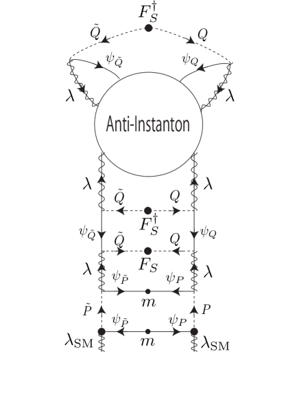
In Fig. 1, we show an example of an anti-instanton diagram which may generate the operator Eq. (53). We have not done the computation of diagrams explicitly, and hence Fig. 1 should be taken only as a schematic picture. The existence of a diagram does not always mean the existence of a non-vanishing operator in SUSY theory, because there is a possibility that cancellation may occur among various diagrams 777See also the footnote 6 in the first paper of Ref. [9]. But the operator Eq. (53) respects all the symmetry of the theory and it is not protected by holomorphy, so there seems to be no mechanism which forbids the existence of the operator. It seems, at the first glance, that Eq. (53) is quite small since it is generated by the anti-instanton effect. However, the contribution Eq. (54) may give not-so-small gaugino masses compared to the sfermion masses, since the gauge coupling is large.
Acknowledgements
We would like to thank K.-I. Izawa and F. Takahashi for the collaboration in the early project, and E. Nakamura for useful discussions on the GUT breaking in semi-direct-type gauge mediation. This work was supported by World Premier International Research Center Initiative (WPI Initiative), MEXT, Japan. The work of KY is supported in part by JSPS Research Fellowships for Young Scientists.
Appendix Appendix A Example of phase transition
To see an example of the phase transition discussed in Section 3.3, let us consider a toy model which have a similarity to our model.
Consider an IYIT model of SUSY breaking [20, 21], with one extra massive flavor 888 This toy model is a simplified version of the model studied by E. Nakamura [22]. We thank him for explanation of his result.. The matter chiral fields of the model are quarks in the fundamental representation of the gauge group, and six singlets . We take the tree level superpotential to be
| (A.1) |
One can easily see an analogy between this toy model and our model, although there is neither a runaway superpotential nor a conformal fixed point in this toy model.
Let us consider two limits of this toy model; and , where is the dynamical scale of the gauge theory. In the following analysis, we neglect any perturbative effects and RG evolution of parameters, and only consider the strong gauge dynamics.
First, consider the limit . In this limit, are massive and they can be integrated out. The low energy theory is the usual IYIT model with the dynamical scale . Confinement occurs and the effective superpotential is given by
| (A.2) |
where are low energy mesons, and is a lagrange multiplier. The equation of motion of gives , then the -term of is . Thus the SUSY is broken by the -term of .
Next consider the limit . In this case, the low energy theory can be described by mesons , , and . The superpotential is,
| (A.3) |
where dots denote terms containing , which are unimportant for the discussion below. The leading terms in the Kähler potential of the low energy theory may be of the form
| (A.4) |
where is a positive numerical constant. Then the potential is
| (A.5) |
where is the totally anti-symmetric tensor with . Using this potential, we can see that the minima of the potential are at with and , if the condition is satisfied. Around , one can see that a phase transition occurs 999 In a parameter region , the meson description becomes worse and the quark description becomes better..
Thus we can conclude that in the limit , the -term of is zero, while in the other limit , the -term of is non-zero. Such a transition may also occur in our model.
References
- [1] K. A. Intriligator, N. Seiberg and D. Shih, JHEP 0604, 021 (2006) [arXiv:hep-th/0602239].
- [2] R. Kitano, H. Ooguri and Y. Ookouchi, arXiv:1001.4535 [hep-th], and references therein.
- [3] K. I. Izawa and T. Yanagida, Prog. Theor. Phys. 114, 433 (2005) [arXiv:hep-ph/0501254]. See also K. I. Izawa, Prog. Theor. Phys. 98, 443 (1997) [arXiv:hep-ph/9704382].
- [4] N. Seiberg, T. Volansky and B. Wecht, JHEP 0811, 004 (2008) [arXiv:0809.4437 [hep-ph]].
- [5] J. L. Jones, Phys. Rev. D 79, 075009 (2009) [arXiv:0812.2106 [hep-ph]].
- [6] R. Sato, T. T. Yanagida and K. Yonekura, arXiv:0910.3790 [hep-ph].
- [7] R. Kitano, H. Ooguri and Y. Ookouchi, Phys. Rev. D 75, 045022 (2007) [arXiv:hep-ph/0612139].
- [8] K. I. Izawa, F. Takahashi, T. T. Yanagida and K. Yonekura, Phys. Rev. D 80, 085017 (2009) [arXiv:0905.1764 [hep-th]]. See also K. I. Izawa, F. Takahashi, T. T. Yanagida and K. Yonekura, Phys. Lett. B 677, 195 (2009) [arXiv:0902.3854 [hep-th]].
- [9] M. Ibe, Y. Nakayama and T. T. Yanagida, Phys. Lett. B 649, 292 (2007) [arXiv:hep-ph/0703110]; M. Ibe, Y. Nakayama and T. T. Yanagida, Phys. Lett. B 671, 378 (2009) [arXiv:0804.0636 [hep-ph]].
- [10] N. Seiberg, Nucl. Phys. B 435, 129 (1995) [arXiv:hep-th/9411149].
- [11] K. A. Intriligator and N. Seiberg, Nucl. Phys. Proc. Suppl. 45BC, 1 (1996) [arXiv:hep-th/9509066].
- [12] N. Arkani-Hamed and H. Murayama, Phys. Rev. D 57, 6638 (1998) [arXiv:hep-th/9705189].
- [13] E. Witten, Nucl. Phys. B 202, 253 (1982).
- [14] I. Affleck, M. Dine and N. Seiberg, Nucl. Phys. B 241, 493 (1984).
- [15] M. Ibe, K. I. Izawa and Y. Nakai, arXiv:0812.4089 [hep-ph]; M. Ibe, K. I. Izawa and Y. Nakai, Phys. Rev. D 80, 035002 (2009) [arXiv:0907.2970 [hep-ph]].
- [16] M. Viel, J. Lesgourgues, M. G. Haehnelt, S. Matarrese and A. Riotto, Phys. Rev. D 71, 063534 (2005) [arXiv:astro-ph/0501562].
- [17] V. A. Novikov, M. A. Shifman, A. I. Vainshtein and V. I. Zakharov, Nucl. Phys. B 229, 381 (1983); M. A. Shifman and A. I. Vainshtein, Nucl. Phys. B 277, 456 (1986) [Sov. Phys. JETP 64, 428 (1986 ZETFA,91,723-744.1986)]; N. Arkani-Hamed and H. Murayama, JHEP 0006, 030 (2000) [arXiv:hep-th/9707133].
- [18] K. A. Intriligator and B. Wecht, Nucl. Phys. B 667, 183 (2003) [arXiv:hep-th/0304128].
- [19] R. Argurio, M. Bertolini, G. Ferretti and A. Mariotti, arXiv:0912.0743 [hep-ph].
- [20] K. I. Izawa and T. Yanagida, Prog. Theor. Phys. 95, 829 (1996) [arXiv:hep-th/9602180].
- [21] K. A. Intriligator and S. D. Thomas, Nucl. Phys. B 473, 121 (1996) [arXiv:hep-th/9603158].
- [22] E. Nakamura, Private communication.