Investigating modularity in the analysis of process algebra models of biochemical systems

Abstract

Compositionality is a key feature of process algebras which is often cited as one of their advantages as a modelling technique. It is certainly true that in biochemical systems, as in many other systems, model construction is made easier in a formalism which allows the problem to be tackled compositionally. In this paper we consider the extent to which the compositional structure which is inherent in process algebra models of biochemical systems can be exploited during model solution. In essence this means using the compositional structure to guide decomposed solution and analysis.

Unfortunately the dynamic behaviour of biochemical systems exhibits strong interdependencies between the components of the model making decomposed solution a difficult task. Nevertheless we believe that if such decomposition based on process algebras could be established it would demonstrate substantial benefits for systems biology modelling. In this paper we present our preliminary investigations based on a case study of the pheromone pathway in yeast, modelling in the stochastic process algebra Bio-PEPA.

1 Introduction

Biochemical systems are generally large and complex and, therefore, studying a biochemical system monolithically can be difficult, both in terms of the definition of the model and in terms of its analysis. Over the last decade process algebras have been proposed as suitable formalisms for constructing models of biochemical systems [21, 23, 20, 9], with their compositional structure being claimed as one of their main advantages.

In many cases the process algebra model is being used as an intermediate language which gives rise to a mathematical representation of the dynamics of the system, on which analysis of the behaviour can be conducted. In many cases this mathematical representation is a stochastic simulation based on an implicit continuous time Markov chain (CTMC), but in others it may be an explicit CTMC, a set of ordinary differential equations (ODEs) or some combination of these. However, regardless of the mathematical formalism chosen, the size and complexity of the biochemical processes can give rise to problems of tractability in the underlying mathematical model. This problem is particularly acute in the case of explicit CTMC models such as those used in probabilistic model-checking. Thus it is attractive to consider the extent to which decomposed model analysis can be used. This approach considers the model to be comprised of a number of modules which may be analysed in isolation, their results being combined to give results for the complete systems. Furthermore when the model has been described in a compositional formalism we would hope that the compositional structure may be exploited in the identification of suitable modules. In this work we refer to process algebras because they are generally equipped with a formal compositional definition, which we can rely on for our modular analysis. It is worth noting, however, that the same approach could potentially be applied to any other language equipped with a notion of modules.

Deriving global dynamic behaviour from the study of isolated components is difficult but the rich potential benefits mean that it has been studied in a wide variety of contexts. For example, notions of modularity and model decomposition have been widely applied in the context of software engineering, network theory and, more recently, systems biology (e.g. [25, 24, 10, 4, 26, 14]). Moreover, model decomposition techniques, such as product form approaches and time scale decomposition, have been defined and applied in the context of CTMC-based analyses and process algebras [15, 16].

However, the full strength of compositionality of process algebra has yet to be used in the context of quantitative analysis of biochemical models, although there have been some attempts to exploit the compositional structure in qualitative analysis and via congruence relations (for example, see [2, 19]). In this paper we present a case study of decomposed model analysis. The system we consider is the yeast pheromone system, previously studied by Kofahl and Klipp [17]. In that paper the authors present an ODE model and an informal decomposition into modules. Here we give a formal model of the system in the stochastic process algebra Bio-PEPA [8, 9] and demonstrate how the compositional structure of the process algebra supports a rigorous definition of modules. Moreover the flexibility of the Bio-PEPA framework to generate a number of different underlying mathematical models allows different analysis techniques to be used in tandem to parameterise and analyse the submodels corresponding to the modules. We choose as our main focus the use of probabilistic model-checking to verify properties of the pathway, partly because this style of analysis is a feature of Bio-PEPA but also because this requires an explicit state space CTMC, so the problem of state space explosion is particularly acute.

As suggested above, we adopt a high-level language, such as Bio-PEPA, instead of considering directly the CTMC model, in order to take advantage of the multiple analysis techniques it supports, since these can be employed in a complementary fashion during model analysis. Specifically, we first use stochastic simulation in order to validate our model against the results in the literature and derive some information necessary for the definition of the associated explicit CTMC submodels. Subsequently, we study further properties of the submodels using model-checking and investigate which properties of the submodels can safely be interpreted in the context of the complete model. It is worth noting that the decomposition of the Bio-PEPA model into modules does not require us to build the full CTMC model, which indeed can be very large and difficult to represent and study explicitly.

The rest of the paper is organised as follows. First, we present a discussion of model decomposition and an overview of our approach (Section 2). In the following section (Section 3) we give a brief introduction to the Bio-PEPA language. Our approach is applied to the yeast pheromone pathway in the following Sections 4 and 5. Some conclusions and future work are reported in Section 6.

2 Decomposing models

As mentioned earlier, a process algebra description of a biochemical pathway can be regarded as an intermediate representation sitting between the biological knowledge and the mathematical models on which analysis is conducted. Consequently the process algebra description plays two roles. Firstly, it is a repository of the current biological knowledge about the system under study. Secondly, it is a specification of the mathematical model which is to be constructed to analyse that system.

When we wish to consider the decomposition of the process algebra model it follows that we may view the problem from the two different perspectives: the biological and the mathematical. In the biological perspective the existence of functional units within biochemical systems is well known. Perhaps the most intuitive examples of this functional separation are signalling pathways, which can be considered as units responsible for conveying specific messages within larger systems. Nevertheless, these modules often affect each other, either positively or negatively, through crosstalk.

Some attempts at defining modules with biochemical systems via biological function have appeared in the literature recently, for instance [26, 14, 4, 25, 24, 10]. In [25, 24, 10] Saez-Rodriguez et al. decompose signalling pathways into modules, study them in isolation using ODE-based analysis and derive global properties of the system from the local behaviours. Their model decomposition approach is based on the structure of biochemical networks, in particular on the definition of “independent units”. The independence of modules is expressed in terms of absence of retroactivity in the interaction between modules. A connection between two modules is retroactivity-free if it does not involve direct interactions in both directions. If there are indirect interactions, such as feedbacks, the connection between modules exhibits weak retroactivity. The input/output behaviour of a retroactivity-free module does not depend on what it is connected to; therefore, if retroactivity-free functional subunits can be identified within a system, we obtain a modularisation in which the independence of modules is inherent to the system’s functional subunits. The notion of modules defined by Bruggeman et al. in [4] is slightly more specific: the authors distinguish between levels and modules. Subunits which only have regulatory interactions (a species in a subunit acts as an enzyme/inhibitor of a reaction within another subunit, i.e. interactions do not involve mass-transfer between subunits) are called levels; instead, subunits whose interactions involve some mass-transfer (a species in a subunit acts as a product/reactant of a reaction within another subunit) are called modules.

In contrast, from the mathematical perspective the decomposition of the system is generally based on notions of interaction and independence at the state level. This is quite different because interactions between states (often based on the count of molecules of each species) are orthogonal to the interactions between species. In this context various decompositional techniques have been proposed in the context of CTMC models and process algebras in order to aid in the solution of large Markov processes [15]. For example product form techniques rely on only restricted forms of state transitions but do mean that important probability measures relating to the whole system can be retrieved exactly from the analysis of modules in isolation. Other decomposition techniques are generally approximate and may involve solution of an aggregated model recording the interactions between modules in addition to the analysis of the isolated modules. One example would be time scale decomposition of the CTMC model: modules are formed by grouping states in the CTMC which can be reached quickly relatively to the transition rates to states in other modules [5].

Of course, ideally we would like these two views of modules arising from a stochastic process algebra model of a biochemical pathway to coincide. One of the objectives of this paper is to investigate the extent to which that occurs by taking a biologically inspired decomposition and studying how well it performs as a mathematical decomposition.

Which ever approach to decomposition we are taking, in a compositional modelling language the task is more straightforward if the boundaries between the modules required for decomposed solution coincide with the boundaries between components used to construct the model. As we will see this is indeed the case of Bio-PEPA models. In our study each module is considered as an individual smaller network: its behaviour in isolation is analysed, and its local properties identified. When looking at one module in isolation, the behaviour of the other modules can be regarded as part of the external environment. Therefore, the effect of changes in the other modules on the module under study must be investigated. This first analysis step allows us to understand in depth the local behaviour of each part of the pathway.

It is a challenge to identify local properties that can help in understanding the behaviour of the full system. The main issue is to understand which properties can be considered and when they can be applied. Structural properties are in general suitable because the structure of the system is not altered by the model composition; dynamic properties, instead, might not be appropriate, because the system’s dynamics is not guaranteed to be preserved by the composition, especially if feedback mechanisms involving different modules are present. In [25, 24, 10], for instance, the authors focus on some properties used in network theory that can be useful also in the context of signalling pathways, such as signal amplitude, signalling time, and signal duration. From the mathematical perspective the focus is generally on the transient and steady state probability distributions over states.

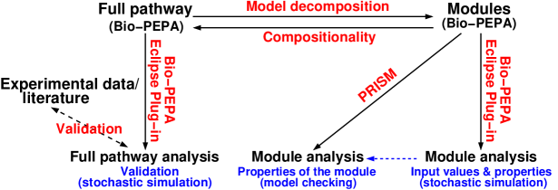
Figure 1: Approach considered in this paper.

As already stated, in our investigation we exploit the compositional and modular structure of Bio-PEPA models and the variety of analysis techniques supported by the language. The schema of the approach considered is reported in Figure 1. We define a Bio-PEPA model for the system and we validate it, as a single entity, against existing data from experiments or literature. The model is then decomposed into modules for detailed analysis, using stochastic simulation and model-checking. The analysis of modules via stochastic simulation is helpful to study some preliminary properties and derive the information needed for CTMC analysis: for this purpose we use the Gibson-Bruck stochastic simulation algorithm [13] available in the Bio-PEPA Eclipse Plug-in [3]. The PRISM model-checker [22] is then used to verify further local properties on the individual modules that can be difficult or impossible to observe directly from stochastic simulation. Moreover, differently from simulation, probabilistic model-checking is an exhaustive approach and, thus, it allows us to simultaneously consider all the possible stochastic behaviours of the modules rather than a finite subset of them. Note that the considered local properties are preserved in the full system, and their verification on the model of the full system is not feasible due to its size.

In order to correctly parameterise the modules in isolation and to interpret the results that we obtain from them, it can be useful to classify the relationship between the modules in terms of their local species and the ones which are on the interface between different modules and act as input/output species. Specifically, when considering a module in isolation, its species can be either (1) local (i.e. not present elsewhere) or (2) involved in reactions occurring in different modules; in the second case, they can act in other modules as either (2a) external regulators (i.e. activators, inhibitors or modifiers) or (2b) external reagents (i.e. products/reactants). Case (2a) corresponds to the notion of level proposed in [4].

When analysing a single module in isolation, this must be parameterised to emulate the effect of the external environment (i.e. the other modules). The hardest case to take into account is when there are species of type (2b), since this means that the amount of the species is changed by the external environment rather than being independently regulated within the considered module. For this type of non-local species, it is crucial to choose appropriate initial values, and additional creation or degradation reactions for such species might be required.

Our objective here is to explore these issues empirically. Based on our experience we believe that an automated procedure could be implemented based on parameter estimation software. This would support finding optimal values for the input/output species and their creation/degradation reactions by comparing the results of the modules in isolation with the results of the whole system and/or experimental data.

3 Bio-PEPA

In this section we give a short description of Bio-PEPA, a language that has recently been developed for the modelling and analysis of biological systems. The interested reader is referred to [8, 9] for more details. The main components of a Bio-PEPA system are the species components, describing the behaviour of each species, and the model component, describing the interactions between the various species. The syntax of Bio-PEPA components is:

$$S::=(\alpha,\kappa)\mbox{ {op} }S\mid S+S\mid C\quad\mbox{with }\texttt{op}=\mbox{$\downarrow$}\mid\mbox{$\uparrow$}\mid\oplus\mid\ominus\mid\odot\quad\quad\quad P::=P\raisebox{-4.30554pt}{$\;\stackrel{{\scriptstyle\mbox{\large$\rhd\!\!\!\!\lhd$}}}{{\scriptscriptstyle\mathcal{I}}}\,$}P\mid S(x)$$

where $S$ is the species component and $P$ is the model component. In the prefix term $(\alpha,\kappa)\mbox{ {op} }S$, $\kappa$ is the stoichiometry coefficient of species $S$ in reaction $\alpha$, and the prefix combinator “op” represents the role of $S$ in the reaction. Specifically, $\downarrow$ indicates a reactant, $\uparrow$ a product, $\oplus$ an activator, $\ominus$ an inhibitor, and $\odot$ a generic modifier. We use the notation “$\alpha\mbox{ {op} }S$” as an abbreviation for “$(\alpha,\kappa)\mbox{ {op} }S$” when $\kappa=1$. The operator “$+$” expresses the choice between possible actions, and the constant $C$ is defined by an equation $C\stackrel{{\scriptstyle\mbox{\em{\tiny def}}}}{{=}}S$. The process $P\raisebox{-4.30554pt}{$\;\stackrel{{\scriptstyle\mbox{\large$\rhd\!\!\!\!\lhd$}}}{{\scriptscriptstyle\mathcal{I}}}\,$}Q$ denotes synchronisation between components $P$ and $Q$, the set $\mathcal{I}$ determines those activities on which the operands are forced to synchronise, with $\;\stackrel{{\scriptstyle\mbox{\large$\rhd\!\!\!\!\lhd$}}}{{\scriptstyle*}}\,$ denoting a synchronisation on all common action types. In $S(x)$ the parameter $x\in{\mathbb{R}}$ represents the initial value for species $S$.

Biological locations (representing both compartments and membranes) can be defined, and the notation $C@L$ indicates that species $C$ is in location $L$. For additional details of the definition of locations see [7]. The formal definition of a Bio-PEPA system is the following.

Definition 1

A Bio-PEPA system $\mathcal{P}$ is a 6-tuple $\langle\mathcal{L},\mathcal{N},\mathcal{K},\mathcal{F}_{R},Comp,P\rangle$, where: $\mathcal{L}$ is the set of locations, $\mathcal{N}$ is an optional set of information for the species, $\mathcal{K}$ is the set of parameters, $\mathcal{F}_{R}$ is the set of functional rates, $Comp$ is the set of species components, and $P$ is the model component.

The language is given a formal, discrete state, small step semantics based on operational rules — see [8, 9] for details. Moreover, mappings have been defined from Bio-PEPA to a variety of underlying mathematical models and analysis techniques — stochastic simulation based on CTMC, ordinary differential equations (ODEs) and probabilistic model-checking. These mappings and the subsequent analyses are supported by various software tools [3, 11, 22]. In the case of numerical analysis of CTMC and probabilistic model-checking using PRISM [18, 22], species are abstracted in terms of levels, each level representing an interval $h$ of values (representing number of molecules, for instance); the set $\mathcal{N}$ specifies the information needed for the derivation of the CTMC with levels, such as the lower and upper bounds on molecular amounts, and the step sizes $h$. In PRISM quantitative properties of the system are expressed using the temporal logic CSL (Continuous Stochastic Logic) [1] and rewards.

4 The yeast pheromone pathway

In order to illustrate our approach, we consider the yeast pheromone pathway in haploid yeast cells after stimulation by $\alpha$-factor [17]. A schema of the pathway together with the definition of modules presented in [17] and discussed below is reported in Figure 2. The receptor Ste2 is activated by the pheromone $\alpha$-factor and in turn activates a heterotrimeric G-protein which transmits the signal from the cell surface receptor to intracellular effectors. In particular, the receptor interacts with some subunits of $G$. This leads to a series of conformational changes, allowing, among others, the release of $G\beta\gamma$. $G\beta\gamma$ binds to and activates a scaffold protein-bound mitogen-activated protein kinase (MAP kinase complex, $C$ in the figure), resulting from the mating pheromone subpathway (top left part in the figure). The activation of the MAPK cascade (from complex $D$ to $G$) follows, together with further intermediate reactions that lead to the activation of nucleic proteins that control transcription and progression in the cell cycle. Specifically, the protein Fus3 is activated by double phosphorylation at the end of the MAPK cascade. Activated Fus3 phosphorylates and regulates various proteins, such as Ste12 and Sst2. The activation of Ste12 leads to the activation of the protein Bar1, which is translocated in the extracellular space and inhibits the activity of the $\alpha$-factor by degradation.

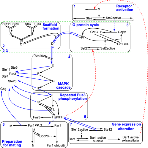
Figure 2: Schema and module decomposition of the yeast pheromone pathway as described in [17]. Black arrows represent interactions which are local to a module, red arrows show feedback loops, blue arrows represent reactions where the outputs of a module are reagents or regulators in another module. Dashed lines of any colour describe regulatory interactions between species whereas solid lines represent interactions involving reagents. The black boxes are the modules defined in [17], and the green dashed box represents the module obtained by merging modules 2 and 3.

We have two feedback loops in the model to take into account:

1. the activated Bar1 in the extracellular space down-regulates the activation of the receptor by enhancing the degradation of the $\alpha$-factor. Bar1 is activated in the last part of the pathway and its quantity is affected by the upstream pathway.

2. Fus3 is activated by double phosphorylation in the last part of the pathway and it is used to activate Sst2; this reduces the quantity of G-protein available for the formation of signalling complexes.

We consider the deterministic model of this pathway defined in [17]. This involves four locations (extracellular space, cytoplasm, cell membrane and nucleus), 35 species and 45 reactions. Most reactions follow the mass-action kinetic law, and a few follow Hill kinetics. The following informal model decomposition of the pathway, driven by the biological meaning of its subparts, is described in [17] and reported schematically in Figure 2 (the modules are represented by the black boxes).

Module 1: Receptor activation.

The pheromone $\alpha$ factor activates the receptor Ste2.

Module 2: Scaffold formation.

Formation of the scaffold complex for the following MAPK cascade.

Module 3: G-protein cycle.

This describes the activity of the G-protein.

Module 4: MAPK cascade.

This module is composed of three phosphorylation steps, and in each of them one species phosphorylates another downstream one. The final result is an active complex containing double phosphorylated Fus3.

Module 5: Repeated Fus3 phosphorylation.

After the MAPK cascade there are a few further reactions that lead to the release of double phosphorylated Fus3.

Module 6: Preparation for mating.

This module describes one of the possible activities influenced by the pheromone pathway.

Module 7: Gene expression alteration.

Phosphorylated Fus3 activates Ste12 that in turn activates Bar1.

According to the described modularisation, modules 2 and 3 are strongly interconnected (via reversible reactions) and, hence, not independent. We consider a modified modularisation, in which modules 2 and 3 are merged in a new module (called module 2-3, the dashed green box in Figure 2) while all other modules are unchanged.

5 Modelling and analysis of the pathway in Bio-PEPA

In this section we show how the pheromone pathway [17] can be modelled exploiting the compositionality offered by the Bio-PEPA language, and we apply decomposed model analysis to the pheromone model. We consider the modules as described in the previous section and we analyse each of them individually. The first issue we need to address in order to analyse modules in isolation is to identify valid initial conditions and parameter values; we show the correctness of the modularisation by comparing the simulation results obtained for the individual models with the ones obtained for the complete model. We also report some results obtained using the PRISM model-checker for the verification of local properties which are valid also globally.

Due to space constraints, we show here the definition and the analysis of two of the modules, i.e. module 1 and module 7, which represent the “start” and the “end” of the signalling pathway, respectively. These modules are interesting because they are interconnected by one of the two feedback loops present in the system. Similar considerations can be used for the other modules to obtain full understanding of the model. The full model is available from [3] and can be directly imported into the Bio-PEPA Eclipse Plug-in. Note that in order to adhere to the syntax of the formal definition of Bio-PEPA as presented in Section 3, the following description is slightly different from the concrete syntax accepted by the tool. The reader is referred to [12] for the details of the syntax and usage of the tool.

Each biochemical species of the pathway is represented by a species component, and each biochemical reaction is described by an action type and it is associated with a functional rate describing its kinetic law. Auxiliary information about species, such as the step size and the maximum molecular count, are defined in the set $\mathcal{N}$. Locations, kinetic parameters, functions and observables can be also defined. The quantitative parameters (kinetic constants and initial values) are the ones used in [17], and are not reported here.

The four different locations relevant to the pathway are abstracted using following set of locations:

$$\mathcal{L}=[\;extra:1\,\mathrm{\mu l},\mathbf{C};\;\ cyto:1\,\mathrm{\mu l},\mathbf{C};\;\ nucl:1\,\mathrm{\mu l},\mathbf{C};\;mem:1\,\mathrm{\mu l},\mathbf{M}\;]\enspace.$$

The model component contains all the species components of the systems with their initial values. Since the model component can be defined in a compositional way, we can represent the full pathway as the composition of the different modules. For each module we consider two subsets of species, namely the local species and the input/output ones. In the next sections we show how each of them is defined for the two considered modules.

5.1 Module 1: activation of the receptor

The first module we consider is the one describing the receptor activation (Figure 3).

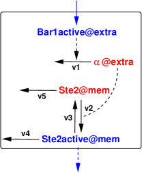
Figure 3: Description of module 1. The species in red are the local species, while the species in blue the external ones. Black arrows are generic reactions in the module whereas the dashed lines represent activation/inhibition. Blue lines are reactions to/from other modules.

The only input species from outside the module is the active extracellular Bar1 ($Bar1active@extra$), generated in module 7, which is an external reagent, whereas the active Ste2 receptor ($Ste2active@mem$) is an external regulator in module 2-3. The local species, which are not influenced by other modules, are the $\alpha$-factor ligand ($\alpha@extra$) and the inactive Ste2 receptor ($Ste2@mem$).

The species definitions for the species of the module are the following

$\alpha@extra$	$\stackrel{{\scriptstyle\mbox{\em{\tiny def}}}}{{=}}$	$v_{1}\,\mbox{$\downarrow$}\,\alpha@extra\;+\;v_{2}\,\oplus\,\alpha@extra$
$Ste2@mem$	$\stackrel{{\scriptstyle\mbox{\em{\tiny def}}}}{{=}}$	$v_{2}\,\mbox{$\downarrow$}\,Ste2@mem\;+\;v_{5}\,\mbox{$\downarrow$}\,Ste2@mem\;+\;v_{3}\,\mbox{$\uparrow$}\,Ste2@mem$
$Ste2active@mem$	$\stackrel{{\scriptstyle\mbox{\em{\tiny def}}}}{{=}}$	$v_{2}\,\mbox{$\uparrow$}\,Ste2active@mem\;+\;v_{4}\,\mbox{$\downarrow$}\,Ste2active@mem\;+\;v_{3}\,\mbox{$\downarrow$}\,Ste2active@mem$
$Bar1active@extra$	$\stackrel{{\scriptstyle\mbox{\em{\tiny def}}}}{{=}}$	$v_{1}\,\oplus\,Bar1active@extra\;+\;v_{38}\,\mbox{$\uparrow$}\,Bar1active@extra$

and the functional rates for these reactions are:

$$f_{v_{1}}=fMA(k_{1});\;\;\;f_{v_{2}}=fMA(k_{2});\;\;\;f_{v_{3}}=fMA(k_{3});\;\;\;f_{v_{4}}=fMA(k_{4});\;\;\;f_{v_{5}}=fMA(k_{5});\;\;\;f_{v_{38}}=fMA(k_{38})$$

where $fMA(r)$ stands for mass-action law with kinetic constant $r$, $v_{1}$ represents the degradation of the $\alpha$-factor, $v_{2}$ the activation of the receptor, $v_{3}$ its deactivation, $v_{4}$ the degradation of the active receptor, $v_{5}$ the degradation of the inactive receptor, and $v_{38}$ the transport of $Bar1active$ from the nucleus to the extracellular space. The parameters $k_{1},\dots,k_{5}$ and $k_{38}$ are defined as in [17].

The model component describing the full module 1 is the following.

$$\begin{array}[]{lcl}Module1\_local\!\!\!&\!\!\!\stackrel{{\scriptstyle\mbox{\em{\tiny def}}}}{{=}}\!\!\!&\!\!\!alpha@extra[init\_alpha\_extra]\raisebox{-4.30554pt}{$\;\stackrel{{\scriptstyle\mbox{\large$\rhd\!\!\!\!\lhd$}}}{{\scriptstyle*}}\,$}Ste2@mem[init\_Ste2\_mem]\\ Module1\_I/O\!\!\!&\!\!\!\stackrel{{\scriptstyle\mbox{\em{\tiny def}}}}{{=}}\!\!\!&\!\!\!Bar1active@extra[init\_Bar1active\_extra]\raisebox{-4.30554pt}{$\;\stackrel{{\scriptstyle\mbox{\large$\rhd\!\!\!\!\lhd$}}}{{\scriptstyle*}}\,$}Ste2active@mem[init\_Ste2active\_mem]\end{array}$$

The initial values are the same as in [17] for all the species except $Bar1active@extra$ which, being an external reagent, deserves further discussion.

Bar1 is inactive in the full pathway, and it is activated and transported into the extracellular environment after the activation of Fus3 by double phosphorylation (in module 7). Reaction $v_{38}$, represents the transport of $Bar1active$ from the nucleus to the extracellular space, which is in the interface between module 7 and module 1. The rate of this reaction depends on the amount of $Bar1active@nucl$, which is not part of this module. Therefore, when considering module 1 in isolation, we need to find an appropriate way to parameterise this reaction, and to assign an initial value to $Bar1active@extra$: these values must be chosen in order to make the behaviour of the species in the module the same as their behaviour in the model of the full pathway.

If we interpret the species $Bar1active@extra$ as an input signal, we can study the effect of varying its value on the behaviour of the module. We consider different possibilities for $Bar1active@extra$, two of which are reported in Figure 4. This figure shows the average stochastic simulation results (over 100 runs) for the species involved in the module when the full pathway is considered (Figure 4(a)), and for the module in isolation (Figures 4(b)–4(c)). When the initial amount of $Bar1active@extra$ is equal to $25$ (half the maximum value of the species obtained from simulation of the whole system in the given interval of time, Figure 4(b)), $Ste2active@mem$ has the expected qualitative behaviour, but the peak is much lower and $Ste2@mem$ does not decrease as expected. On the other hand, under the assumption that $Bar1active@extra$ is initially absent and it is created with a constant rate equal to $1.66$ (Figure 4(c)), the results for the module are in perfect agreement with the results obtained for the full pathway. The use of a creation reaction for $Bar1active@extra$ is motivated by the fact that in the full pathway this species grows linearly in the time interval considered: by simulating the full pathway model, we observe that at time $t=30$ it reaches the value $50$. Therefore, its behaviour can be approximated well by a creation reaction with rate $50/30=1.66$.

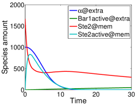
(a) Full pathway

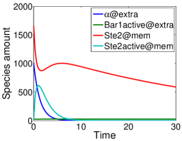
(b) $init\_Bar1active@extra=25$

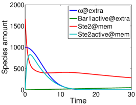
(c) Creation rate $k_{0}=1.66$

Figure 4: Module 1: Time-series evolution (Gibson-Bruck method, average of 100 simulation runs) of the involved species for different assumptions about $Bar1active@extra$: (a) full pathway, (b) module 1, with initial amount of $Bar1active@extra=25$, and (c) module 1, with $Bar1active@extra$ initially absent and created with rate $k_{0}=1.66$.

In order to study some further properties of the module, we consider the corresponding PRISM model. We use the simulation results to derive the maximum amounts for the species, and we define the step sizes $h_{1}=10$ for $Bar1active@extra$ and $h_{2}=50$ for all the other species. The maximum numbers of levels, derived from the species’ maximum amounts and the step sizes, are $35$ for $Ste2@mem$, $20$ for $\alpha@extra$, $17$ for $Ste2active@mem$, and $5$ for $Bar1active@extra$. Figure 5 reports the computed expected values for all the species in order to validate our PRISM model against the anticipated behaviour. The results are in agreement with the simulation results reported in Figure 4(a) and the results in the literature [17]. Some small discrepancies are due to the choice of the step size. Indeed a finer granularity gives better results, but the chosen one is enough to obtain some information about the module.

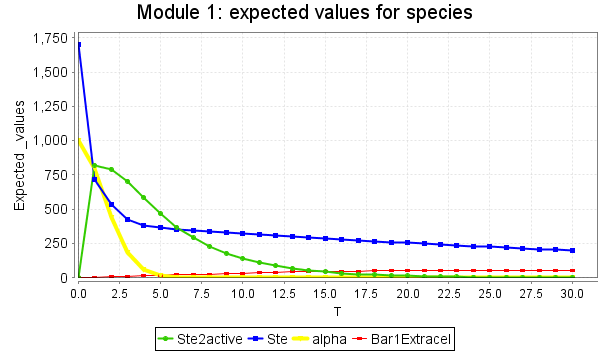
Figure 5: Module 1: Expected values for the amounts of the involved species computed in PRISM using instantaneous reward properties.

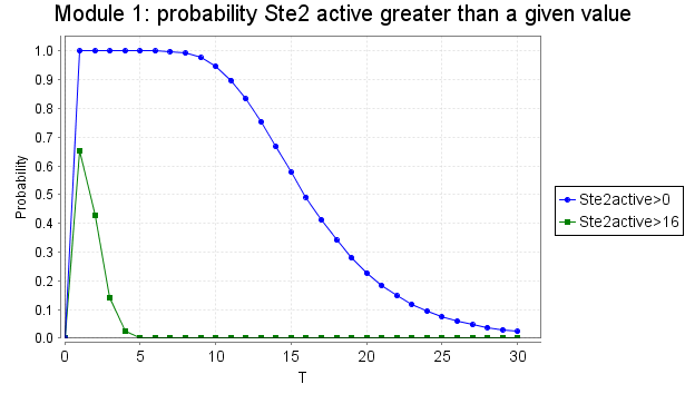
(a) Prob $Ste2active@mem>0$, $Ste2active@mem>16$

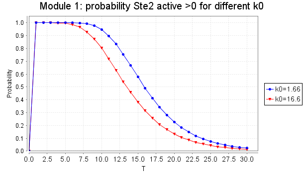
(b) Effect of $k_{0}$ on Prob $Ste2active@mem>0$

Figure 6: Module 1: (a) comparison of the probability of the amount of $Ste2active@mem$ being greater than level zero and greater than level 16; (b) comparison of the probability of the amount of $Ste2active@mem$ being greater than zero for different values of $k_{0}$ (creation rate of $Bar1active@extra$).

Some properties verified using PRISM are reported in Figures 6 and 7. We verify the probability of $Ste2active@mem$ being greater than level zero and greater than 16 (with level 17 corresponding to the maximum concentration for $Ste2active@mem$) (Figure 6(a)), and the probability of $Ste2active@mem$ being greater than zero for different values of the creation rate $k_{0}$ (Figure 6(b)). Concerning the first two probabilities (Figure 6(a)), in the former case the probability rapidly grows to one and then decreases quite slowly to zero, whereas in the latter case we soon have a peak and then the probability rapidly decreases to zero. Indeed the activation of $Ste2active@mem$ happens at the beginning of the pathway and then $Ste2active@mem$ is degraded and not created anymore. Concerning the effect on $Ste2active@mem$ of changing $k_{0}$ (Figure 6(b)), the first part is the same for all the assumptions, but then a larger creation rate leads to a faster decrease of the probability. The last properties we analyse regard the ratio of $Ste2active@mem$ to $Ste2\_total=Ste2active@mem+Ste2@mem$ (Figure 7(a)) and the expected number of reactions that have been fired within a given time (Figure 7(b)).

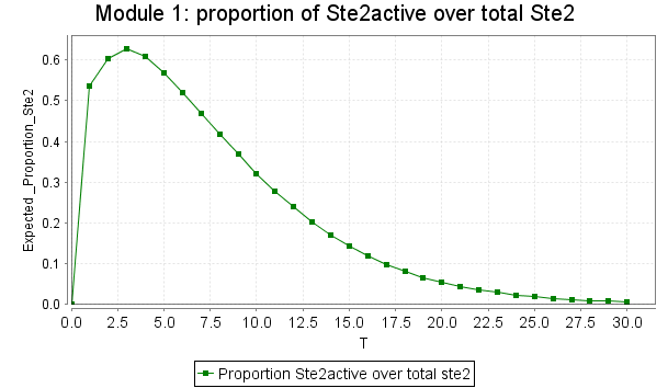
(a) $Ste2active@mem/Ste2\_total$

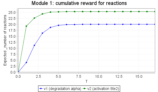
(b) Reaction occurrences

Figure 7: Module 1: (a) ratio of amount of $Ste2active@mem$ to total amount of Ste2 ($Ste2active@mem+Ste2@mem$); (b) expected number of reaction occurrences.

Most of the properties reported above for module 1 are valid for the full model too and so they can be used to derive global properties for the pathway. Indeed the results presented for this module are in agreement with the expected behaviour of the species in the module when considering the full pathway. This is not true when experimenting with parameter values in the module. Indeed a change in the parameters can lead to a variation in the amount of some species in other modules (such as $Bar1active@extra$) and this can have an effect on the modules themselves.

5.2 Module 7: gene alteration

The second module considered in this paper is the one describing gene alteration (Figure 8).

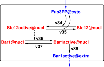
Figure 8: Description of module 7.

This module is slightly more complex than the previous one, because the input $Fus3PP@cyto$ is involved in several modules: in addition to being both a reactant and a product here, $Fus3PP@cyto$ is both reactant and product in module 5 and has a regulatory role in modules 2-3 and 6. However, the value of $Fus3PP@cyto$ is unaffected by those modules and therefore its regulatory role in other modules is not an issue. The other species of this module are $Bar1active@extra$ which, as we saw in the previous section, has a regulatory effect in module 1, and four local species: nucleic Ste12 in inactive ($Ste12@nucl$) and active ($Ste12active@nucl$) forms, and nucleic Bar1 in inactive ($Bar1@nucl$) and active ($Bar1active@nucl$) forms.

The species definitions for the species of the module are the following

$Fus3PP@cyto$	$\stackrel{{\scriptstyle\mbox{\em{\tiny def}}}}{{=}}$	$v_{46}\,\oplus\,Fus3PP@cyto\;+\;v_{28}\,\mbox{$\uparrow$}\,Fus3PP@cyto\;+\;v_{33}\,\mbox{$\downarrow$}\,Fus3PP@cyto$
		$v_{39}\,\oplus\,Fus3PP@cyto\;+\;v_{35}\,\mbox{$\uparrow$}\,Fus3PP@cyto\;+\;v_{34}\,\mbox{$\downarrow$}\,Fus3PP@cyto$
$Ste12@nucl$	$\stackrel{{\scriptstyle\mbox{\em{\tiny def}}}}{{=}}$	$v_{35}\,\mbox{$\uparrow$}\,Ste12@nucl\;+\;v_{34}\,\mbox{$\downarrow$}\,Ste12@nucl$
$Ste12active@nucl$	$\stackrel{{\scriptstyle\mbox{\em{\tiny def}}}}{{=}}$	$v_{35}\,\mbox{$\downarrow$}\,Ste12active@nucl\;+\;v_{34}\,\mbox{$\uparrow$}\,Ste12active@nucl\;+\;v_{36}\,\oplus\,Ste12active@nucl$
$Bar1@nucl$	$\stackrel{{\scriptstyle\mbox{\em{\tiny def}}}}{{=}}$	$v_{36}\,\mbox{$\downarrow$}\,Bar1@nucl\;+\;v_{37}\,\mbox{$\uparrow$}\,Bar1@nucl$
$Bar1active@nucl$	$\stackrel{{\scriptstyle\mbox{\em{\tiny def}}}}{{=}}$	$v_{38}\,\mbox{$\downarrow$}\,Bar1active@nucl\;+\;v_{37}\,\mbox{$\downarrow$}\,Bar1active@nucl\;+\;v_{36}\,\mbox{$\uparrow$}\,Bar1active@nucl$
$Bar1active@extra$	$\stackrel{{\scriptstyle\mbox{\em{\tiny def}}}}{{=}}$	$v_{38}\,\mbox{$\uparrow$}\,Bar1active@extra\;+\;v_{1}\,\oplus\,Bar1active@extra$

and the model component describing the full module 7 is the following.

$$\begin{array}[]{lcl}Module7\_local\!\!&\!\!\stackrel{{\scriptstyle\mbox{\em{\tiny def}}}}{{=}}\!\!&\!\!Ste12@nucl[init\_Ste12\_nucl]\raisebox{-4.30554pt}{$\;\stackrel{{\scriptstyle\mbox{\large$\rhd\!\!\!\!\lhd$}}}{{\scriptstyle*}}\,$}Ste12active@nucl[init\_Ste12active\_nucl]\raisebox{-4.30554pt}{$\;\stackrel{{\scriptstyle\mbox{\large$\rhd\!\!\!\!\lhd$}}}{{\scriptstyle*}}\,$}\\ \!\!&\!\!\!\!&\!\!Bar1@nucl[init\_Bar1\_nucl]\raisebox{-4.30554pt}{$\;\stackrel{{\scriptstyle\mbox{\large$\rhd\!\!\!\!\lhd$}}}{{\scriptstyle*}}\,$}Bar1active@nucl[init\_Bar1active\_nucl]\\ Module7\_I/O\!\!&\!\!\stackrel{{\scriptstyle\mbox{\em{\tiny def}}}}{{=}}\!\!&\!\!Fus3PP@cyto[init\_Fus3PP\_cyto]\raisebox{-4.30554pt}{$\;\stackrel{{\scriptstyle\mbox{\large$\rhd\!\!\!\!\lhd$}}}{{\scriptstyle*}}\,$}Bar1active@extra[init\_Bar1active\_extra]\end{array}$$

As for the previous module, we have to assign a value for the external reagent $Fus3PP@cyto$: we study the effect of its variation on the behaviour of the module, and find an appropriate value for which we can reproduce the results obtained on the full pathway model. In Figure 9 we report the average stochastic simulation results (over 100 runs) for all the species involved in this module when the full pathway is considered (Figure 9(a)), and for the module in isolation (Figures 9(b)–9(c)). Both when $Fus3PP@cyto$ is initially 300 (the maximum value it attains in the full pathway, Figure 9(b)) and when it is initially 150 (half its maximum value, Figure 9(c)), the behaviour of Bar1 in all its forms is the same as the one obtained in the full pathway; however, only using the initial value 300 the module behaves exactly as the full pathway also in terms of the amounts $Ste12@nucl$ and $Ste12active@nucl$.

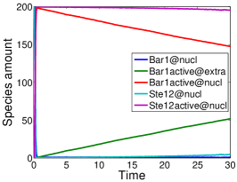
(a) Full pathway

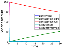
(b) $init\_Fus3PP@cyto=300$

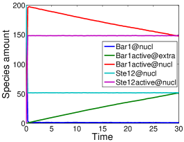
(c) $init\_Fus3PP@cyto=150$

Figure 9: Module 7: Time-series evolution (Gibson-Bruck method, average of 100 simulation runs) of the involved species for different assumptions about $Fus3PP@cyto$: (a) full pathway, (b) module 1, with initial amount of $Fus3PP@cyto=300$, and (c) module 1, with initial amount of $Fus3PP@cyto=150$.

We again use PRISM to analyse the CTMC with levels associated with the module in order to verify the satisfaction of a few desired properties. Given the maximum amount derived from simulation, we define the step size $h=25$. The resulting maximum number of levels is $12$ for $Fus3PP@cyto$ and $8$ for the other species. Figures 10, 11, and 12 report some results obtained from the analysis in PRISM. In Figure 10 the expected values for the amounts of the species are shown; these are in agreement with the simulation results. Figure 11 reports the probability of $Ste12active@nucl$ being greater than level zero (Figure 11(a)), and the ratio of $Ste12active@nucl$ to $Ste12\_total=Ste12@nucl+Ste12active@nucl$ (Figure 11(b)). The probability of $Ste12active@nucl$ being greater than zero increases rapidly from zero to one and the ratio has a similar behaviour. Indeed, Ste12 is converted rapidly from the inactive state to the active state and the inactivation reaction is very slow compared with the activation one. Figure 12 describes the probability of the expected value of $Bar1active@extra$ being greater than zero under different assumptions about the transport rate. As expected, increasing the transport rate constant makes the probability grow more rapidly to the value one. These properties, verified locally for the module, are valid also for the full system.

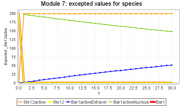
Figure 10: Module 7: Expected values for the amounts of the involved species computed using PRISM.

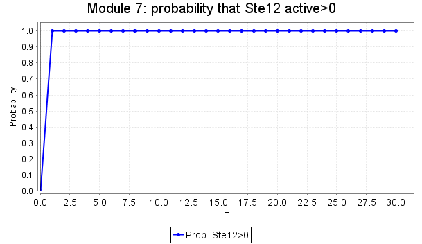
(a) Prob $Ste12active@nucl>0$

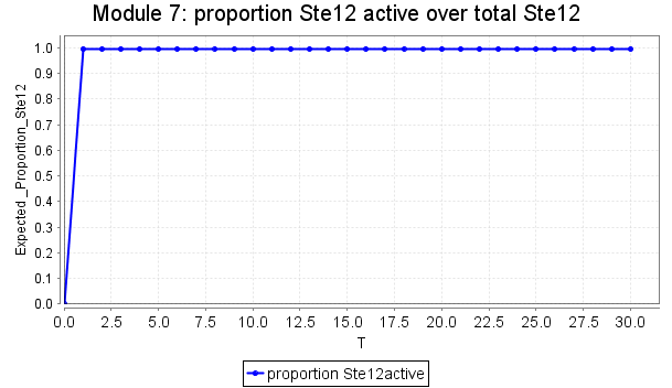
(b) $Ste12active@nucl/Ste12\_total$

Figure 11: Module 7: (a) probability of $Ste12active@nucl$ being greater than zero; (b) ratio of amount of $Ste12active@nucl$ to total amount of Ste12 ($Ste12@nucl+Ste12active@nucl$).

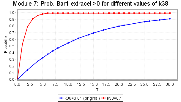
Figure 12: Module 7: probability of $Ste12active@nucl$ being greater than zero for different values of the transport rate $k_{38}$. The original value ($k_{38}=0.01$, blue line) and $k_{38}=0.1$ (red line) are considered.

6 Conclusions

Compositionality is a key feature of process algebras and can offer several advantages in terms of both model construction and model analysis, especially in the context of biological modelling. Indeed biological systems are generally large and complex and inherently characterised by a modular structure. Whereas there are numerous explorations of compositional modelling using process algebras, the application of compositionality for system analysis has not been widely investigated.

Here we presented a preliminary study of decomposed model analysis for biochemical systems specified in the Bio-PEPA process algebra. We focused on the pheromone pathway in yeast, characterised by a modular structure reflecting biological functionalities, and we applied a modular approach for the analysis. The approach proposed was illustrated for a single case study, but the potential advantages, especially with respect to the increased feasibility and efficiency of the analysis techniques, are evident. In particular, the modular analysis allowed us to benefit from analysis techniques, such as model-checking, whose application to the analysis of the full system would be unfeasible due to the state-space explosion.

This work highlighted that the definition of a general approach for decomposed model analysis can be very useful. However this task is challenging and several issues must be addressed. The most important of these is the identification of suitable modules. We have shown that modules do not need to be independent. Here we assumed that the modules can be defined based on pre-existing biological knowledge of the system, but it is necessary to define a general technique. Our examples suggest that the fine-grained modularity of the reagent-centric modelling style supported by Bio-PEPA [6], offers sufficient flexibility to support decomposition according to a wide-range of criteria. Secondly, modules must be correctly parameterised for them to be analysed in isolation. Here the correctness of the modularisation and the parameterisation is performed by visual inspection of the simulation traces obtained for the individual and the complete model; the application for this purpose of classical techniques for model distance and of formal relations (e.g. congruences) offered by process algebra is potentially interesting. Finally, the class of system properties which can be verified locally and are also guaranteed to hold for the full system must be characterised. These are the main issues we are planning to investigate in future work.

Our emphasis has been on biological decomposition and which gives rise to a rather ad hoc mathematical decomposition. Nevertheless we have shown that useful modular analysis can be carried out. Another area for future work would be to start from the underlying mathematical model, i.e. the CTMC, and apply established mathematical decomposition techniques and investigate the implication for decomposition at the biological level.

References

- [1] A. Aziz, K. Sanwal, V. Singhal, and R. Brayton. Verifying continuous time Markov chains. Proc. 8th International Conference on Computer Aided Verification (CAV’96), LNCS, 1102:269–276, 1996.
- [2] R. Barbuti, A. Maggiolo-Schettini, P. Milazzo, and A. Troina. Bisimulations in calculi modelling membranes. Formal Aspects of Computing, 20(4-5):351–377, 2008.
- [3] Bio-PEPA Home Page. http://www.biopepa.org/.
- [4] F.J. Bruggeman, J.L. Snoep, and H.V. Westerhoff. Control, responses and modularity of cellular regulatory networks: a control analysis perspective. IET Syst Biol., 2(6):397–410, 2008.
- [5] H. Busch, W. Sandmann, and V. Wolf. A Numerical Aggregation Algorithm for the Enzyme-Catalyzed Substrate Conversion. In Proc. of CMSB’06, volume 4210 of LNCS, pages 298–311. Springer, 2006.
- [6] M. Calder and J. Hillston. Process algebra modelling styles for biomolecular processes. Trans. on Computational Systems Biology, XI(LNBI 5750):1–25, 2009.
- [7] F. Ciocchetta and M.L. Guerriero. Modelling Biological Compartments in Bio-PEPA. In Proc. of MeCBIC’08, volume 227 of ENTCS, pages 77–95, 2009.
- [8] F. Ciocchetta and J. Hillston. Bio-PEPA: an extension of the process algebra PEPA for biochemical networks. In Proc. of FBTC’07, volume 194 of ENTCS, pages 103–117, 2008.
- [9] F. Ciocchetta and J. Hillston. Bio-PEPA: a Framework for the Modelling and Analysis of Biological Systems. Theoretical Computer Science, 410(33–34):3065–3084, 2009.
- [10] H. Conzelmann, J. Saez-Rodriguez, T. Sauter, E. Bullinger, F. Allgöwer, and E.D. Gilles. Reduction of mathematical models of signal transduction networks: simulation-based approach applied to EGF receptor signalling. Systems Biology, 1(1):159–169, 2004.
- [11] Dizzy Home Page. http://magnet.systemsbiology.net/software/Dizzy.
- [12] A. Duguid. An overview of the Bio-PEPA Eclipse Plug-in. In Proc. of PASTA’09, 2009.
- [13] M.A. Gibson and J. Bruck. Efficient Exact Stochastic Simulation of Chemical Systems with Many Species and Many Channels. The Journal of Chemical Physics, 104:1876–1889, 2000.
- [14] L.H. Hartwell, J.J. Hopfield, S. Leibler, and A.W. Murray. From molecular to modular cell biology. Nature, 402:C47–C52, 1999.
- [15] J. Hillston. Lectures on Formal Methods and Performance Analysis, volume 2090 of LNCS, chapter Exploiting Structure in Solution: Decompositing Compositional Models. Springer-Verlag, 2001.
- [16] J. Hillston and V. Mertsiotakis. A Simple Time Scale Decomposition Technique for Stochastic Process Algebras. Comput. J., 38(7):566–577, 1995.
- [17] B. Kofahl and E. Klipp. Modelling the dynamics of the yeast pheromone pathway. Yeast, 21:831–850, 2004.
- [18] M. Kwiatkowska, G. Norman, and D. Parker. PRISM: Probabilistic Model Checking for Performance and Reliability Analysis. ACM SIGMETRICS Performance Evaluation Review, 2009.
- [19] M.C. Pinto, L. Foss, J.C.M. Mombach, and L. Ribeiro. Modelling, property verification and behavioural equivalence of lactose operon regulation. Computers in Biology and Medicine, 37:134–148, 2007.
- [20] C. Priami and P. Quaglia. Operational patterns in Beta-binders. Transactions on Computational Systems Biology, 1:50–65, 2005.
- [21] C. Priami, A. Regev, W. Silverman, and E. Shapiro. Application of a stochastic name-passing calculus to representation and simulation of molecular processes. Information Processing Letters, 80(1):25–31, 2001.
- [22] PRISM Home Page. http://www.prismmodelchecker.org.
- [23] A. Regev, E.M. Panina, W. Silverman, L. Cardelli, and E.Y. Shapiro. BioAmbients: an Abstraction for Biological Compartments. Theoretical Computer Science, 325(1):141–167, 2004.
- [24] J. Saez-Rodriguez, H. Conzelmann, K. Bettenbrock, A. Kremling, and E.D. Gilles. Modular Analysis of Signal Transduction Networks. IEEE control Systems Magazine, 2004.
- [25] J. Saez-Rodriguez, A. Kremling, and E.D. Gilles. Dissecting the puzzle of life: modularization of signal transduction networks. Computers and Chemical Engineering, 29:619–629, 2005.
- [26] V.M. Wolf and A.P. Arkin. Motifs, modules and games in bacteria. Current opinion in Microbiology, 6:125–13, 2003.