Spin fluctuations and superconductivity in noncentrosymmetric heavy fermion systems CeRhSi₃ and CeIrSi₃

Abstract

We study the normal and the superconducting properties in noncentrosymmetric heavy fermion superconductors CeRhSi₃ and CeIrSi₃. For the normal state, we show that experimentally observed linear temperature dependence of the resistivity is understood through the antiferromagnetic spin fluctuations near the quantum critical point (QCP) in three dimensions. For the superconducting state, we derive a general formula to calculate the upper critical field $H_{c2}$, with which we can treat the Pauli and the orbital depairing effect on an equal footing. The strong coupling effect for general electronic structures is also taken into account. We show that the experimentally observed features in $H_{c2}\parallel\hat{z}$, the huge value up to $30$(T), the downward curvatures, and the strong pressure dependence, are naturally understood as an interplay of the Rashba spin-orbit interaction due to the lack of inversion symmetry and the spin fluctuations near the QCP. The large anisotropy between $H_{c2}\parallel\hat{z}$ and $H_{c2}\perp\hat{z}$ is explained in terms of the spin-orbit interaction. Furthermore, a possible realization of the Fulde-Ferrell- Larkin-Ovchinnikov state for $H\perp\hat{z}$ is studied. We also examine effects of spin-flip scattering processes in the pairing interaction and those of the applied magnetic field on the spin fluctuations. We find that the above mentioned results are robust against these effects. The consistency of our results strongly supports the scenario that the superconductivity in CeRhSi₃ and CeIrSi₃ is mediated by the spin fluctuations near the QCP.

I Introduction

In noncentrosymmetric heavy fermion superconductors, in addition to strong electron correlation, there exists another key property, the anisotropic spin-orbit (SO) interaction due to the lack of inversion symmetry. The anisotropic SO interaction plays important roles both in the normal and the superconducting state, and is expected to lead to many interesting phenomena. pap:Edelstein89 ; pap:Edelstein95 ; pap:Yip ; pap:Gorkov ; pap:Frigeri ; pap:Samokhin04 ; pap:Samokhin05 ; pap:Mineev05 ; pap:Mineev07 For such phenomena, electron correlation is quite important, because it can largely enhance the effect of the SO interaction. The interplay of the anisotropic SO interaction and electron correlation is truly an unique nature in noncentrosymmetric heavy fermion compounds. pap:FujimotoPRB ; pap:FujimotoJPSJ1 ; pap:FujimotoJPSJ2 In particular, such an interplay in the superconducting state has been attracting particular interest. In this context, especially, CeRhSi₃ pap:Kimura ; pap:Muro ; pap:KimuraJPSJ and CeIrSi₃ pap:Sugitani ; pap:Okuda are promising candidates for the interplay, because they are considered to be located near the antiferromagnetic (AF) QCPs around which strong correlations through the spin fluctuations are essential.

CeRhSi₃ and CeIrSi₃ are AF metals at ambient pressure, and begin to exhibit superconductivity at some critical pressures $P_{c}$ where the Néel temperatures seem to be suppressed to absolute zero. According to the neutron experiments for CeRhSi₃, the AF ordering vector is $\mbox{\boldmath$Q$}=(\pm 0.43\pi,0,0.5\pi),(0,\pm 0.43\pi,0.5\pi)$ and the nature of the AF order is spin density wave-like. pap:Aso This is different from CePt₃Si in which the AF seems to have localized nature and the superconductivity coexists with it even at zero applied pressure. pap:Bauer In NMR experiments in CeIrSi₃, $1/T_{1}\propto T/(T+\theta)^{1/2}$ is observed near the critical pressure, which is a characteristic behavior of the systems with 3-dimensional (3D) AF spin fluctuations. pap:Mukuda ; pap:SCR1 ; pap:SCR2 In addition, the resistivity $\rho$ in both CeRhSi₃ and CeIrSi₃ above the superconducting transition temperatures $T_{c}$ in some pressure regions near the QCP shows the anomalous $T$-linear dependence which is different from $\rho\sim T^{2}$ in canonical Fermi liquids. pap:KimuraJPSJ ; pap:Sugitani

The QCP related phenomena are observed also in the superconducting state. The large jump in the heat capacity at $T_{c}$ in CeIrSi₃ can be attributed to the strong coupling effect due to the spin fluctuations. pap:Tateiwa It has strong pressure dependence and is largely enhanced near $P_{c}$. The most striking phenomena which would be related to the quantum criticality in CeRhSi₃ and CeIrSi₃ appear in the behaviors of the upper critical fields $H_{c2}$ when the applied magnetic field is parallel to $z$-axis. pap:Kimura_Hc2 ; pap:Settai The remarkable features of the experimental results are as follows. (i) As the pressure approaches a critical value, $H_{c2}$ exhibits extremely high value which exceeds the orbital limit as well as the Pauli limit estimated by the conventional BCS theory. The observed $H_{c2}\sim 30$(T) is the highest value among the heavy fermion superconductors ever discovered, although $T_{c}$ is merely $T_{c}\sim 1$(K). (ii) $H_{c2}$ curves have downward curvatures and the increase is accelerated as the temperature is decreased, making a sharp contrast to any other superconductors in which the increase of $H_{c2}$ becomes slower as $T$ is decreased. (iii) $H_{c2}$ increases very rapidly as the pressure approaches the critical value, while the pressure dependence of $T_{c}$ is moderate. These characteristic features strongly suggest that there exists a deep connection between the superconductivity and the magnetic quantum criticality. In the previous study, the present authors have shown that these experimental results are well explained as an interplay of the Rashba SO interaction due to the lack of inversion symmetry and the spin fluctuations near the QCP. pap:TadaPRL

On the other hand, $H_{c2}$ for in-plane fields differs from $H_{c2}\parallel\hat{z}$ in some important features. $H_{c2}\perp\hat{z}$ is merely less than $10$(T) and its pressure dependence is moderate, and the $H_{c2}$ curves exhibit usual upward curvatures. pap:Kimura_Hc2 ; pap:Settai This anisotropy in $H_{c2}$ would be related to the Rashba SO interaction, since the Fermi surface is asymmetrically distorted by the in-plane field and the Pauli depairing effect plays essential roles. By contrast, the renormalization of the quasiparticle velocity by the spin fluctuations is almost isotropic, resulting in the enhanced orbital limiting field in all directions of the applied field. Another interesting phenomenon in the noncentrosymmetric superconductors in applied magnetic fields is the helical vortex phase which has been discussed theoretically.  pap:Kaur ; pap:Yanase ; pap:Dimitrova ; pap:Agterberg ; pap:Samokhin ; pap:Matsunaga ; pap:Hiasa ; pap:Mineev In a helical vortex phase, the superconducting gap function is modulated in real space, $\Delta(\mbox{\boldmath$R$})\sim\exp(i\mbox{\boldmath$Q$}\cdot\mbox{\boldmath$R$})\Delta$ with the modulation vector $Q\sim(\alpha/\varepsilon_{F})\mu_{B}H/v_{F}$, where $\alpha,v_{F},\varepsilon_{F}$ and $\mu_{B}$ are the strength of the SO interaction, the Fermi velocity, the Fermi energy, and the Bohr magneton, respectively. For 3D Rashba superconductors for $H\perp\hat{z}$, however, it is pointed out that this phase modulation is just a translational shift of the vortex lattice and has no physical importance. pap:Matsunaga ; pap:Hiasa ; pap:Mineev Several authors also have discussed a spatially modulated superconducting state under magnetic fields with a large $Q\sim\mu_{B}H/v_{F}$ which is continuously connected from $Q\sim(\alpha/\varepsilon_{F})\mu_{B}H/v_{F}$. pap:Yanase ; pap:Dimitrova ; pap:Samokhin ; pap:Hiasa This large $Q$ state corresponds to the Fulde-Ferrell-Ovchinnikov-Larkin (FFLO) state. pap:FF ; pap:LO The stability of the modulating superconducting state with the large $Q$ depends on the relative strength of the orbital depairing effect to the Pauli depairing effect in the compounds.

In this paper, we study the normal and the superconducting properties in noncentrosymmetric superconductors CeRhSi₃ and CeIrSi₃. We examine the anomalous $T$-linear dependence of the resistivity in the normal state. In the previous studies,pap:SCR1 ; pap:SCR2 at very low temperatures, $\rho\sim T^{3/2}$ is predicted for 3D AF spin fluctuations. The temperature dependence of the resistivity for 3D AF spin fluctuations have been studied in detail by several authors pap:Rosch ; pap:RoschPRB ; pap:Onari We, here, show that $\rho\sim T$ in CeRhSi₃ and CeIrSi₃ is actually due to the 3D AF spin fluctuations. For the superconducting state, the upper critical fields both for $H\parallel\hat{z}$ and $H\perp\hat{z}$ are investigated. For the calculation of $H_{c2}$, we derive a general formula which enables us to treat the Pauli and the orbital depairing effects on an equal footing. We can also take into account the strong coupling effect for a given electronic structure. We calculate $H_{c2}$ on the basis of the scenario that the superconductivity in CeRhSi₃ and CeIrSi₃ is mediated by the spin fluctuations, and show that the experimental features are well explained as an interplay of the spin fluctuations and the Rashba SO interaction. Although the formula is applicable for general models, we use a phenomenological model to calculate $H_{c2}$ and neglect the following two points in the model. One is the scattering processes in the pairing interaction in which spins of quasiparticles are flipped by the Rashba SO interaction. It is pointed out that such processes can enhance the admixture of the singlet and the triplet superconductivity, pap:Yanase08 ; pap:Takimoto and the strength of the admixture affects $H_{c2}\perp\hat{z}$. pap:Hiasa We show that the admixture is still small in CeRhSi₃ and CeIrSi₃ even if we include the spin-flip scattering processes. The other point is the applied field dependence of the spin fluctuations. Because the applied field is so large in CeRhSi₃ and CeIrSi₃ especially for $H\parallel\hat{z}$ that one might think that the spin fluctuations are suppressed and they cannot contribute to the enhancement of $H_{c2}$. We show that the spin fluctuations are robust against the applied field $H$ up to the strength of the Rashba SO interaction, $\mu_{B}H\lesssim\alpha$, because the Rashba SO interaction tends to fix the directions of spins on the Fermi surface and it competes with the Zeeman effect. The consistency of our results with the experiments strongly supports the scenario that the superconductivity in CeRhSi₃ and CeIrSi₃ is mediated by the spin fluctuations near the AF QCP.

This paper is organized as follows. In Sec.II, we study the experimentally observed $T$-linear dependence of the resistivity. In Sec.III, a general formula for the calculation of $H_{c2}$ is derived from the Eliashberg equation. The characteristic features of $H_{c2}$ in CeRhSi₃ and CeIrSi₃ are well explained with the use of the formula in Sec.IV. We discuss, in Sec.V, the spin-flip scattering processes in the pairing interaction and the magnetic field dependence of the spin fluctuations which are not included in the approximation used for the computation of $H_{c2}$. The summary is given in Sec.VI.

II resistivity in normal state

In this section, we discuss the temperature dependence of the resistivity near the AF QCP in CeRhSi₃ and CeIrSi₃. In CeIrSi₃, NMR $1/T_{1}$ behaves as $1/T_{1}\propto T/\sqrt{T+\theta}$ in some pressure regions, which means that the character of the spin fluctuations is 3D antiferromagnetic. pap:Mukuda ; pap:SCR1 ; pap:SCR2 In noncentrosymmetric systems, however, spin fluctuations are not isotropic due to the anisotropic spin-orbit interaction. The anisotropy in the noninteracting susceptibility $\hat{\chi}^{0}$ is of the order of $\alpha/\varepsilon_{F}\ll 1$, where $\alpha$ is the strength of the spin-orbit interaction and $\varepsilon_{F}$ is the Fermi energy. Actually, in Sec.V.2, we show that the anisotropy among $\chi_{xx},\chi_{yy}$ and $\chi_{zz}$ is very small within the random phase approximation. Therefore, we can neglect the anisotropy of the spin fluctuations for the discussion of the resistivity and $H_{c2}$ in CeRhSi₃ and CeIrSi₃.

For the systems with 3D AF spin fluctuations, the resistivities are expected to be $\rho\sim T^{3/2}$ according to the previous studies. pap:SCR1 ; pap:SCR2 In CeRhSi₃ and CeIrSi₃, however, the temperature dependence is $\rho\sim T$ near the AF QCP. pap:KimuraJPSJ ; pap:Sugitani The resistivity due to the 3D AF spin fluctuations was discussed by several authors, and $\rho\sim T$ behavior was found for the weakly disordered systems pap:Rosch ; pap:RoschPRB and the clean systems. pap:Onari Here, we show that the $T$-linear resistivity in CeRhSi₃ and CeIrSi₃ is naturally understood in terms of the 3D AF spin fluctuations, and this behavior has basically nothing to do with the lack of inversion symmetry.

CeRhSi₃ and CeIrSi₃ are heavy fermion systems with Kondo temperature $T_{\rm K}\sim$50-100(K) which is much higher than the superconducting transition temperature $T_{c}\sim 1$(K). pap:Kimura ; pap:Sugitani ; pap:Muro98 Therefore, to study the properties at $T=$1-10(K), we consider the low energy quasiparticles mainly formed by $f$-electrons through the hybridizations with the conduction electrons. We use the following single band model for the low energy quasiparticles with the asymmetric spin-orbit interaction

$$S = S_{0}+S_{\rm SF},$$ (1)

$$S_{0} = \sum_{k}c^{\dagger}_{k}[-i\omega_{n}+\varepsilon_{0}(\mbox{\boldmath$k$})]c_{k}+\sum_{k}c^{\dagger}_{k}\alpha\mbox{\boldmath$\mathcal{L}$}_{0}(\mbox{\boldmath$k$},\mbox{\boldmath$H$})\cdot\mbox{\boldmath$\sigma$}c_{k},$$ (2)

$$S_{\rm SF} = -\sum_{kk^{\prime}q}\frac{g^{2}}{6}\chi(q)\mbox{\boldmath$\sigma$}_{\alpha\alpha^{\prime}}\cdot\mbox{\boldmath$\sigma$}_{\beta\beta^{\prime}}c^{\dagger}_{k+q\alpha}c_{k\alpha^{\prime}}c^{\dagger}_{k^{\prime}-q\beta}c_{k^{\prime}\beta^{\prime}},$$ (3)

where $c_{k\sigma}^{(\dagger)}$ is the annihilation (creation) operator of the Kramers doublet of the $\Gamma_{7}$ state. $S_{\rm SF}$ is introduced phenomenologically and represents the interaction between the quasiparticles by the strong spin fluctuations near the AF QCP. Since CeRhSi₃ and CeIrSi₃ have body-centered tetragonal lattice structures with lattice spacing $1:1:2$, pap:Muro ; pap:Okuda the dispersion relation $\varepsilon_{0}(\mbox{\boldmath$k$})$ and the Rashba type SO interaction are approximated by

$$\varepsilon_{0}(\mbox{\boldmath$k$}) = -2t_{1}(\cos k_{x}a+\cos k_{y}a)+4t_{2}\cos k_{x}a\cos k_{y}a$$ (4)

$$-8t_{3}\cos(k_{x}a/2)\cos(k_{y}a/2)\cos k_{z}a-2t_{4}\cos 2k_{z}a-\mu,$$

$$\mbox{\boldmath$\mathcal{L}$}_{0}(\mbox{\boldmath$k$},\mbox{\boldmath$H$}) = (\sin k_{y}a,-\sin k_{x}a-\mu_{B}H_{y}/\alpha,-\mu_{B}H_{z}/\alpha),$$ (5)

where $a$ is the lattice constant and $\mu$ is the chemical potential. Although $\mbox{\boldmath$H$}=0$ in this section, we include the Zeeman effect in the action for the later discussion. We fix the parameters as $(t_{1},t_{2},t_{3},t_{4},n,\alpha)=(1.0,0.475,0.3,0.0,1.0,0.5)$ by taking $t_{1}$ as the energy unit. The Fermi surface determined by these parameters is in qualitative agreement with the band calculation and can reproduce the peak structures of the momentum-dependent susceptibility observed by the neutron scattering experiments pap:Aso ; pap:TadaJPSJ ; pap:Harima . Since we consider $f$-electron systems, we assume that the above parameters include effects of the mass renormalization due to local spin correlations with typical energy scale $T_{\rm K}\sim$ 50-100 (K), the Kondo temperature; i.e. $t_{1}\sim$ 50-100 (K).

The interactions are phenomenologically introduced through the renormalized susceptibility $\chi(q)$, pap:SCR1 ; pap:SCR2 ; pap:TadaPRL ; pap:Monthoux92 ; pap:Monthoux99

$$\chi(i\nu_{n},\mbox{\boldmath$q$}) = \sum_{a}\frac{\chi_{0}\xi^{2}q_{0}^{2}}{1+\xi^{2}(\mbox{\boldmath$q$}-\mbox{\boldmath$Q$}_{a})^{2}+|\nu_{n}|/(\Gamma_{0}\xi^{-2}q_{0}^{-2})},$$ (6)

$$\xi(T,\theta) = \tilde{\xi}\sqrt{\frac{t_{1}}{T+\theta}},$$ (7)

where $\chi_{0}$, $q_{0}$ and $\Gamma_{0}$ are respectively the susceptibility, the length scale and the energy scale of spin fluctuations without strong correlations. These quantities are renormalized through the coherence length $\xi(T)$ as the system approaches the QCP. The critical exponent of $\xi$ is the mean field value $1/2$ and $\theta$ is considered to decrease monotonically as the applied pressure approaches the critical value for the AF order. pap:SCR1 ; pap:SCR2 The temperature dependence of $\xi$ is also consistent with the recent NMR experiment for CeIrSi₃. pap:Mukuda The ordering vectors are $\mbox{\boldmath$Q$}_{1}=(\pm 0.43\pi,0,0.5\pi)/a,\mbox{\boldmath$Q$}_{2}=(0,\pm 0.43\pi,0.5\pi)/a$ according to the neutron scattering experiments for CeRhSi₃. pap:Aso In this study, we fix the parameters in $\chi(i\nu_{n},\mbox{\boldmath$q$})$ as $q_{0}=a^{-1}$, $\Gamma_{0}=3.6t_{1}$ and $\tilde{\xi}=0.45a$. The value $\Gamma_{0}=3.6t_{1}$ is of the same order as the Fermi energy without the effect of the spin fluctuations. $\tilde{\xi}$ is determined so that the maximum of $\xi$ would be $\xi_{\rm max}\lesssim 10a$ at the lowest temperature in this study, which is a reasonable value for the AF spin fluctuations. We note that the coupling constant $g$ should be regarded as an effective one renormalized by the vertex corrections. pap:Yonemitsu ; pap:Monthoux_ver

The Green’s function is, pap:FujimotoPRB ; pap:FujimotoJPSJ1 ; pap:FujimotoJPSJ2

$$G_{\alpha\beta}(k) = \sum_{\tau=\pm 1}l_{\tau\alpha\beta}(k)G_{\tau}(k),$$ (8)

$$l_{\tau\alpha\beta}(k) = \frac{1}{2}\left(1+\tau\hat{\mbox{\boldmath$\mathcal{L}$}}(k)\cdot\mbox{\boldmath$\sigma$}\right)_{\alpha\beta},$$ (9)

$$G_{\tau}(k) = \frac{1}{i\omega_{n}-\varepsilon_{\tau}(k)-\Sigma_{0}(k)}$$ (10)

where $\varepsilon_{\tau}(k)=\varepsilon_{0}(\mbox{\boldmath$k$})+\tau\alpha\|\mbox{\boldmath$\mathcal{L}$}(k)\|,\mbox{\boldmath$\mathcal{L}$}(k)=\mbox{\boldmath$\mathcal{L}$}_{0}(\mbox{\boldmath$k$})+\mbox{\boldmath$\Sigma$}(k)/\alpha,\mbox{\boldmath$\hat{\mathcal{L}}$}(k)=\mbox{\boldmath$\mathcal{L}$}(k)/\|\mbox{\boldmath$\mathcal{L}$}(k)\|$ and $\|\mbox{\boldmath$\mathcal{L}$}(k)\|=\sqrt{\sum_{i=1}^{3}[{\mathcal{L}}_{i}(k)]^{2}}$. Selfenergy is introduced as $\Sigma_{0}=(\Sigma_{\uparrow\uparrow}+\Sigma_{\downarrow\downarrow})/2,\Sigma_{x}=(\Sigma_{\downarrow\uparrow}+\Sigma_{\uparrow\downarrow})/2,\Sigma_{y}=(\Sigma_{\downarrow\uparrow}-\Sigma_{\uparrow\downarrow})/2i,$ and $\Sigma_{z}=(\Sigma_{\uparrow\uparrow}-\Sigma_{\downarrow\downarrow})/2.$ Up to the first order in $g^{2}\chi_{0}$, $\Sigma_{0}$ and $\Sigma$ are expressed as

$$\Sigma_{0}(k) = \frac{T}{2N}\sum_{k^{\prime}}g^{2}\chi(k-k^{\prime})[G^{0}_{\uparrow\uparrow}(k^{\prime})+G^{0}_{\downarrow\downarrow}(k^{\prime})],$$ (11)

$$\Sigma_{x}(k) = \frac{T}{2N}\sum_{k^{\prime}}\frac{g^{2}}{3}\chi(k-k^{\prime})[-G^{0}_{\downarrow\uparrow}(k^{\prime})-G^{0}_{\uparrow\downarrow}(k^{\prime})],$$ (12)

$$\Sigma_{y}(k) = \frac{T}{2iN}\sum_{k^{\prime}}\frac{g^{2}}{3}\chi(k-k^{\prime})[-G^{0}_{\downarrow\uparrow}(k^{\prime})+G^{0}_{\uparrow\downarrow}(k^{\prime})],$$ (13)

$$\Sigma_{z}(k) = \frac{T}{2N}\sum_{k^{\prime}}\frac{g^{2}}{3}\chi(k-k^{\prime})[-G^{0}_{\uparrow\uparrow}(k^{\prime})+G^{0}_{\downarrow\downarrow}(k^{\prime})]$$ (14)

where $G^{0}_{\alpha\beta}$ is the non-interacting Green’s function. We have neglected the constant terms in $\Sigma_{\mu}$. In the above expression of $\Sigma_{\mu}$, the most dominant term is $\Sigma_{0}$, and $\Sigma_{x,y}$ is smaller than $\Sigma_{0}$ by the factor $\alpha/\varepsilon_{F}\ll 1$, where $\varepsilon_{F}$ is the Fermi energy. For Rashba superconductors, $\Sigma_{z}=0$ without magnetic field.

The conductivity is calculated from the Kubo formula

$$\sigma_{\mu\nu} = \lim_{\omega\rightarrow 0}\frac{1}{\omega}{\rm Im}K_{\mu\nu}^{R}(\omega),$$ (15)

$$K_{\mu\nu}(i\omega_{n}) = \int_{0}^{\beta}d\tau e^{i\omega_{n}\tau}\langle TJ_{\mu}(\tau)J_{\nu}(0)\rangle,$$ (16)

where the current operator $J_{\mu}$ is defined as

$$J_{\mu} = e\sum_{k}c_{k}^{\dagger}\hat{v}_{k\mu}c_{k},$$ (17)

$$\hat{v}_{k\mu} = \nabla_{\mu}[\varepsilon_{0}(\mbox{\boldmath$k$})+\alpha\mbox{\boldmath$\mathcal{L}$}_{0}(\mbox{\boldmath$k$})\cdot\mbox{\boldmath$\sigma$}].$$ (18)

After the analytic continuation, $G^{A}_{\tau}G^{R}_{\tau^{\prime}}$ has the dominant contribution to the conductivity. Among the four terms $\{G^{A}_{\tau}G^{R}_{\tau^{\prime}}\}_{\tau,\tau^{\prime}=\pm 1}$, for sufficiently large $\alpha$, the terms $G^{A}_{+}G^{R}_{-}$ and $G^{A}_{-}G^{R}_{+}$ have no singularity with respect to the quasiparticle damping rate. Therefore, we can neglect them, and the resulting expression for $\sigma_{xx}$ is

$$\sigma_{xx} = e^{2}\sum_{k,\tau}{\rm tr}[\hat{v}_{kx}\hat{l}^{A}_{k\tau}\hat{v}_{kx}\hat{l}^{R}_{k\tau}]\left(-\frac{\partial f}{\partial\varepsilon}(\varepsilon_{k\tau})\right)\frac{1}{2\gamma_{k\tau}},$$ (19)

$$\gamma_{k\tau} = -[{\rm Im}\Sigma_{0}^{\rm R}(0,\mbox{\boldmath$k$})+\tau{\rm Re}\hat{\mbox{\boldmath$\mathcal{L}$}}^{R}(0,\mbox{\boldmath$k$})\cdot{\rm Im}\mbox{\boldmath$\Sigma$}^{R}(0,\mbox{\boldmath$k$})]$$ (20)

where ${\rm Re}\hat{\mbox{\boldmath$\mathcal{L}$}}^{R}={\rm Re}\mbox{\boldmath$\mathcal{L}$}^{R}/\|{\rm Re}\mbox{\boldmath$\mathcal{L}$}^{R}\|$, $l^{(R,A)}_{k\tau}=l^{(R,A)}_{\tau}(\varepsilon_{k\tau},\mbox{\boldmath$k$})$ and $\varepsilon_{k\tau}=\varepsilon_{\tau}(\mbox{\boldmath$k$})+{\rm Re}\Sigma_{0}(0,\mbox{\boldmath$k$})$. Here we have neglected the vertex corrections which are necessary for the current conservation law. pap:Eliashberg ; pap:Yamada ; pap:Kontani ; book:Yamada This is because, for the resistivity, the scatterings by the AF spin fluctuations have large momentum transfers, and therefore, the back-flow included in the vertex corrections does not affect the temperature dependence of the resistivity. book:Yamada As mentioned above, $\Sigma$ is much smaller than $\Sigma_{0}$ in amplitude, and from Eqs.(11) $\sim$(14), the temperature dependence of $\Sigma_{0}$ and that of $\Sigma$ are the same. Therefore, hereafter, we neglect $\Sigma$ and take into account only $\Sigma_{0}$ in this study. The resistivity in noncentrosymmetric systems is almost the same as that in usual centrosymmetric systems. This is different from the situations for the anomalous Hall effect, the magnetoelectric effect and so on for which the Rashba SO interaction plays important roles. pap:Edelstein95 ; pap:Yip ; pap:FujimotoPRB ; pap:FujimotoJPSJ1 ; pap:FujimotoJPSJ2

Before moving to the numerical calculation, we show a simple analytical result for ${\rm Im}\Sigma_{0}$ which determines the qualitative behavior of $\sigma_{\mu\nu}$. Since Eq.(11) is basically the same as the selfenergy $\Sigma_{\rm cen}$ in the usual centrosymmetric systems, we consider $\Sigma_{\rm cen}$ for brevity. The selfenergy at the hot spots for a sufficiently clean system with the impurity damping $\gamma_{\rm imp}\ll v_{F}/\xi$ is calculated as

$${\rm Im}\Sigma_{\rm cen}^{R}(0,\mbox{\boldmath$k$}_{F}) = g^{2}\sum_{q}\int_{-\infty}^{\infty}\frac{d\varepsilon}{2\pi}\Bigl{[}\coth\frac{\varepsilon}{2T}-\tanh\frac{\varepsilon}{2T}\Bigr{]}{\rm Im}\chi^{R}(\varepsilon,\mbox{\boldmath$q$}){\rm Im}G^{0R}_{\rm cen}(\varepsilon,\mbox{\boldmath$k$}_{F}-\mbox{\boldmath$q$})$$ (21)

$$\sim \sum_{q}\frac{\chi_{Q}\Gamma_{s}(\pi T)^{2}}{\omega_{q}(\omega_{q}+\pi T/2)}{\rm Im}G^{0R}_{\rm cen}(0,\mbox{\boldmath$k$}_{F}-\mbox{\boldmath$q$})$$

$$\sim \xi^{0}T\ln\bigl{[}1+\pi T/2\Gamma_{s}\bigr{]},$$

where $G^{0R}$ is the retarded Green’s function including the impurity damping $\gamma_{\rm imp}$ and $\chi^{R}$ is the retarded susceptibility obtained from the analytic continuation of Eq.(6). In the above calculation, the dispersion at the hot spots has been expanded as $\varepsilon_{0}(\mbox{\boldmath$k$}_{F}-\mbox{\boldmath$q$})=\nabla\varepsilon_{0}(\mbox{\boldmath$k$}_{F}-\mbox{\boldmath$Q$})\cdot(\mbox{\boldmath$Q$}-\mbox{\boldmath$q$})$ for $\mbox{\boldmath$q$}\simeq\mbox{\boldmath$Q$}$, because $\varepsilon_{0}(\mbox{\boldmath$k$}_{F}-\mbox{\boldmath$Q$})=-\varepsilon_{0}(\mbox{\boldmath$k$}_{F})=0$ is satisfied at the hot spots. Here, we have used the approximation $H(z)\equiv\int d\varepsilon[\coth(\varepsilon/2T)-\tanh(\varepsilon/2T)]\varepsilon/(\omega_{q}^{2}+\varepsilon^{2})=1/z-2[\psi(z+1)-\psi(z+1/2)]\simeq(\pi T)^{2}/[\omega_{q}(\omega_{q}+\pi T/2)]$, where $\psi$ is digamma function and $z=\omega_{q}/(2\pi T)$. pap:Kontani ; pap:Stojkovic This approximate form becomes exact both for $z\rightarrow 0$ and $z\rightarrow\infty$. $\chi_{Q},\Gamma_{s}$ and $\omega_{q}$ are defined as $\chi_{Q}=\chi_{0}(\xi q_{0})^{2},\Gamma_{s}=\Gamma_{0}(\xi q_{0})^{-2}$ and $\omega_{q}=\Gamma_{s}[1+\xi^{2}(\mbox{\boldmath$q$}-\mbox{\boldmath$Q$})^{2}]$, respectively. Therefore, we have $\rho\sim-{\rm Im}\Sigma^{R}\sim T$ when the hot spots are dominant for the conductivity. This is a general behavior for the clean 3D systems with the 3D AF spin fluctuations.

In the numerical calculation, we neglect the real part of the selfenergy which changes the shape of the Fermi surface, because such an effect is non-perturbative. We regard $\varepsilon_{\tau}(\mbox{\boldmath$k$})$ as the dispersion that includes ${\rm Re}\Sigma_{0}$. We show the numerical results for $\rho_{xx}=1/\sigma_{xx}$ by using Eq.(11) and Eq.(19) for clean limit.

Figure 1: Resistivity v.s. temperature for several $\theta$. From the top to the bottom, $\theta/t_{1}=0.002,0.05,0.2$.

As shown in Fig.1, for sufficiently small $\theta$, the resistivity is proportional to $T$ in a wide range of temperature where the hot spots are thermally blurred and dominant for the conductivity. In a very low temperature region where such blurring is suppressed, $\rho$ is dominated by the electrons in the cold spots. For large $\theta$, the canonical Fermi liquid behavior $\rho\sim T^{2}$ can be seen. The calculated $\rho$ well explains the experimentally observed features of the resistivity in CeRhSi₃ and CeIrSi₃. Therefore, we conclude that the observed $\rho\sim T$ above $T_{c}$ is due to the AF spin fluctuations.

We put a remark on the impurity effect. pap:Rosch ; pap:RoschPRB If the impurity scattering is sufficiently strong, the anisotropic scatterings by the spin fluctuations are smeared, which weakens the singularity. We, here, simply estimate the selfenergy by the spin fluctuations $\Sigma_{\rm cen}^{\rm sf}$ in the presence of the impurities for centrosymmetric systems analytically. For the system with the strong impurity effect which smears the anisotropy by the AF spin fluctuations, we evaluate the selfenergy $\Sigma_{\rm cen}^{\rm sf}$ averaged on the Fermi surface

$$\langle{\rm Im}\Sigma^{{\rm sf}R}_{\rm cen}(0,\mbox{\boldmath$k$})\rangle_{\rm FS} \equiv \frac{\sum_{k}{\rm Im}\Sigma^{{\rm sf}R}_{\rm cen}(0,\mbox{\boldmath$k$}){\rm Im}G^{0R}_{\rm cen}(0,\mbox{\boldmath$k$})}{\sum_{k}{\rm Im}G^{0R}_{\rm cen}(0,\mbox{\boldmath$k$})}$$ (22)

$$\propto \sum_{q}\frac{\chi_{Q}\Gamma_{s}(\pi T)^{2}}{\omega_{q}(\omega_{q}+\pi T/2)}\frac{\partial{\rm Im}\chi^{0R}_{\rm cen}(0,\mbox{\boldmath$q$})}{\partial\omega}$$

$$\sim \xi^{-1}T\left(\sqrt{1+\pi T/2\Gamma_{s}}-1\right),$$

where we have defined $\chi^{0}_{\rm cen}(q)=-(T/N)\sum_{k}G^{0}_{\rm cen}(k)G^{0}_{\rm cen}(k+q)$. Here, we have assumed that its $T,q$-dependence is moderate and it does not contribute to the selfenergy. We obtain $\rho\sim T^{3/2}$ for $\xi^{-2}\sim T$ in dirty systems. Note that, in the case of $\xi^{-2}\sim T^{3/2}$, we again have $\xi^{-1}T\left(\sqrt{1+\pi T/2\Gamma_{s}}-1\right)\sim T^{3/4}T^{1}T^{-1/4}=T^{3/2}$ for sufficiently low temperatures. Thus, the resistivity in the dirty systems with 3D AF spin fluctuations is $\rho\sim T^{3/2}$ both for $\xi^{-2}\sim T$ and $\xi^{-2}\sim T^{3/2}$ in agreement with the previous studies. pap:SCR1 ; pap:SCR2

III Eliashberg equation in magnetic field

III.1 exact formula within semiclassical approximation

In this section, we derive a formula for the calculation of $H_{c2}$ from the linearized Eliashberg equation in real space. The derivation is based on the semiclassical approximation which is legitimate for the systems with $k_{F}l_{H}\gg 1$, where $k_{F}$ is the Fermi wave number and $l_{H}=1/\sqrt{|e|H}$ is the magnetic length. This condition is satisfied for many superconductors including heavy fermion superconductors, and therefore, the resulting equation for $H_{c2}$ is applicable for a number of compounds. Our formula is a generalization of the previous studies, pap:WHH ; pap:Schossmann ; pap:Bulaevskii and can be extended easily to more complicated models although we use a single band model in this section.

To derive the formula for the calculation of $H_{c2}$, we use the linearized Eliashberg equation in real space with the vector potential $A$ which gives a uniform magnetic field,

$$\Delta_{\alpha\alpha^{\prime}}(i\omega_{n},\mbox{\boldmath$x$},\mbox{\boldmath$x$}^{\prime};\mbox{\boldmath$A$}) = -\frac{1}{\beta}\sum_{i\omega_{m}}\sum_{\mbox{\boldmath$y$}\mbox{\boldmath$y$}^{\prime}}V_{\alpha\alpha^{\prime},\beta\beta^{\prime}}(i\omega_{n},\mbox{\boldmath$x$},\mbox{\boldmath$x$}^{\prime};i\omega_{m},\mbox{\boldmath$y$},\mbox{\boldmath$y$}^{\prime};\mbox{\boldmath$A$})$$ (23)

$$\times\sum_{\mbox{\boldmath$z$}\mbox{\boldmath$z$}^{\prime}}G_{\beta\gamma}(i\omega_{m},\mbox{\boldmath$y$},\mbox{\boldmath$z$};\mbox{\boldmath$A$})\Delta_{\gamma\gamma^{\prime}}(i\omega_{m},\mbox{\boldmath$z$},\mbox{\boldmath$z$}^{\prime};\mbox{\boldmath$A$})G_{\beta^{\prime}\gamma^{\prime}}(-i\omega_{m},\mbox{\boldmath$y$}^{\prime},\mbox{\boldmath$z$}^{\prime};\mbox{\boldmath$A$}),$$

where $\sum_{x}$ represents the summation over all lattice sites, and the spin indices are summed over. $G,\Delta$ and $V$ are, respectively, the normal Green’s function, the gap function and the pairing interaction. Note that, if $A$ is fully taken into account in the above equation, the resulting equation is gauge invariant under the gauge transformation $\mbox{\boldmath$A$}(\mbox{\boldmath$x$})\rightarrow\mbox{\boldmath$A$}(\mbox{\boldmath$x$})+\nabla f(\mbox{\boldmath$x$})$ and $\psi(\tau,\mbox{\boldmath$x$})\rightarrow\exp[ief(\mbox{\boldmath$x$})]\psi(\tau,\mbox{\boldmath$x$})$ where $\psi$ is the field operator of the electrons. By this transformation, each factor in the equation acquires the additional phases as,

$$G(i\omega_{n},\mbox{\boldmath$x$},\mbox{\boldmath$x$}^{\prime}) \rightarrow \exp[ie\left(f(\mbox{\boldmath$x$})-f(\mbox{\boldmath$x$}^{\prime})\right)]G(i\omega_{n},\mbox{\boldmath$x$},\mbox{\boldmath$x$}^{\prime}),$$ (24)

$$\Delta(i\omega_{n},\mbox{\boldmath$x$},\mbox{\boldmath$x$}^{\prime}) \rightarrow \exp[ie\left(f(\mbox{\boldmath$x$})+f(\mbox{\boldmath$x$}^{\prime})\right)]\Delta(i\omega_{n},\mbox{\boldmath$x$},\mbox{\boldmath$x$}^{\prime}),$$ (25)

$$V(i\omega_{n},\mbox{\boldmath$x$},\mbox{\boldmath$x$}^{\prime};i\omega_{m},\mbox{\boldmath$y$},\mbox{\boldmath$y$}^{\prime}) \rightarrow \exp[ie\left(f(\mbox{\boldmath$x$})+f(\mbox{\boldmath$x$}^{\prime})-f(\mbox{\boldmath$y$})-f(\mbox{\boldmath$y$}^{\prime})\right)]V(i\omega_{n},\mbox{\boldmath$x$},\mbox{\boldmath$x$}^{\prime};i\omega_{m},\mbox{\boldmath$y$},\mbox{\boldmath$y$}^{\prime}).$$ (26)

In this study, however, we use the semiclassical approximation in which we do not explicitly include the effect of the vector potential on the pairing interaction $V$, because the vector potential in $V$ is not responsible for the Landau quantization of the gap function which is the most important phenomenon of the orbital effect in type-II superconductors. By contrast, the lack of translational invariance in $G$ and $\Delta$ in the presence of the applied vector potential $A$ is related to the Landau quantization. Within the semiclassical approximation, the normal Green’s function is

$$G(i\omega_{n},\mbox{\boldmath$x$},\mbox{\boldmath$y$};\mbox{\boldmath$A$}) = e^{i\varphi(\mbox{\boldmath$x$},\mbox{\boldmath$y$})}G(i\omega_{n},\mbox{\boldmath$x$}-\mbox{\boldmath$y$};\mbox{\boldmath$A$}=0),$$ (27)

$$\varphi(\mbox{\boldmath$x$},\mbox{\boldmath$y$}) = e\int_{\mbox{\boldmath$y$}}^{\mbox{\boldmath$x$}}\mbox{\boldmath$A$}(\mbox{\boldmath$s$})d\mbox{\boldmath$s$}.$$ (28)

We can easily perform the integral along the straight line $\mbox{\boldmath$s$}(t)=\mbox{\boldmath$y$}+t(\mbox{\boldmath$x$}-\mbox{\boldmath$y$}),0\leq t\leq 1$, using the relation $\mbox{\boldmath$A$}(a\mbox{\boldmath$x$}+b\mbox{\boldmath$y$})=a\mbox{\boldmath$A$}(\mbox{\boldmath$x$})+b\mbox{\boldmath$A$}(\mbox{\boldmath$x$})$ which holds for any $A$ giving a uniform magnetic field $H$, and obtain

$$\varphi(\mbox{\boldmath$x$},\mbox{\boldmath$y$})=e\mbox{\boldmath$A$}\left(\frac{\mbox{\boldmath$x$}+\mbox{\boldmath$y$}}{2}\right)\cdot(\mbox{\boldmath$x$}-\mbox{\boldmath$y$}).$$ (29)

Although the linearized Eliashberg equation is no longer invariant under the gauge transformation defined above within this approximation, it is still gauge invariant under a gauge transformation which involves only the center of mass coordinate of the Cooper pairs.

Next, we proceed to rewrite Eq.(23) in $k$-space. The pairing interaction $V$ should be decomposed into two parts as,

$$V(i\omega_{n},\mbox{\boldmath$x$},\mbox{\boldmath$x$}^{\prime};i\omega_{m},\mbox{\boldmath$y$},\mbox{\boldmath$y$}^{\prime})=V^{{\rm rel}}(i\omega_{n},\mbox{\boldmath$x$}-\mbox{\boldmath$x$}^{\prime};i\omega_{m},\mbox{\boldmath$y$}-\mbox{\boldmath$y$}^{\prime})\times V^{{\rm cen}}\left(\frac{\mbox{\boldmath$x$}+\mbox{\boldmath$x$}^{\prime}}{2};\frac{\mbox{\boldmath$y$}+\mbox{\boldmath$y$}^{\prime}}{2}\right)$$ (30)

where $V^{{\rm rel}}$ and $V^{{\rm cen}}$ are the interactions in the relative coordinate and the center of mass coordinate. Here, we take $V^{{\rm cen}}$ to be dimensionless. It is convenient to introduce the following variables

$$\begin{split}&\mbox{\boldmath$R$}=\frac{\mbox{\boldmath$x$}+\mbox{\boldmath$x$}^{\prime}}{2},\quad\mbox{\boldmath$r$}=\mbox{\boldmath$x$}-\mbox{\boldmath$x$}^{\prime},\\ &\mbox{\boldmath$Y$}=\mbox{\boldmath$y$}-\mbox{\boldmath$z$},\quad\mbox{\boldmath$Y$}^{\prime}=\mbox{\boldmath$y$}^{\prime}-\mbox{\boldmath$z$}^{\prime},\\ &\mbox{\boldmath$R$}^{\prime}=\frac{\mbox{\boldmath$z$}+\mbox{\boldmath$z$}^{\prime}}{2},\quad\mbox{\boldmath$r$}^{\prime}=\mbox{\boldmath$z$}-\mbox{\boldmath$z$}^{\prime}.\end{split}$$ (31)

In this coordinate, the phase factor $\exp(i\varphi(\mbox{\boldmath$y$},\mbox{\boldmath$z$})+i\varphi(\mbox{\boldmath$y$}^{\prime},\mbox{\boldmath$z$}^{\prime}))$ which arises from $G(i\omega_{m},\mbox{\boldmath$y$},\mbox{\boldmath$z$})G(-i\omega_{m},\mbox{\boldmath$y$}^{\prime},\mbox{\boldmath$z$}^{\prime})$ in Eq.(23) becomes

$$\varphi(\mbox{\boldmath$y$},\mbox{\boldmath$z$})+\varphi(\mbox{\boldmath$y$}^{\prime},\mbox{\boldmath$z$}^{\prime}) = e\mbox{\boldmath$A$}(\mbox{\boldmath$R$}^{\prime})(\mbox{\boldmath$Y$}+\mbox{\boldmath$Y$}^{\prime})+e\mbox{\boldmath$A$}(\mbox{\boldmath$r$}^{\prime})(\mbox{\boldmath$Y$}-\mbox{\boldmath$Y$}^{\prime})+e\mbox{\boldmath$A$}(\mbox{\boldmath$Y$})\mbox{\boldmath$Y$}+e\mbox{\boldmath$A$}(\mbox{\boldmath$Y$}^{\prime})\mbox{\boldmath$Y$}^{\prime}$$

$$\simeq 2e\mbox{\boldmath$A$}(\mbox{\boldmath$R$}^{\prime})\frac{\mbox{\boldmath$Y$}+\mbox{\boldmath$Y$}^{\prime}}{2}+e\mbox{\boldmath$A$}(\mbox{\boldmath$Y$})\mbox{\boldmath$Y$}+e\mbox{\boldmath$A$}(\mbox{\boldmath$Y$}^{\prime})\mbox{\boldmath$Y$}^{\prime}.$$

In the second equality, the neglected term $e\mbox{\boldmath$A$}(\mbox{\boldmath$r$}^{\prime})(\mbox{\boldmath$Y$}-\mbox{\boldmath$Y$}^{\prime})$ is much smaller than the first term, since for the dominant scattering processes, $\|\mbox{\boldmath$Y$}-\mbox{\boldmath$Y$}^{\prime}\|,\|\mbox{\boldmath$r$}^{\prime}\|\ll\|\mbox{\boldmath$Y$}+\mbox{\boldmath$Y$}^{\prime}\|$ are satisfied in the systems with short range pairing interaction. The first term represents the phase which the Cooper pair with center of mass $\mbox{\boldmath$R$}^{\prime}$ acquires. We perform the Fourier transformation of Eq.(23) and assume $V^{{\rm cen}}_{\alpha\alpha^{\prime},\beta\beta^{\prime}}\left(\mbox{\boldmath$R$};\mbox{\boldmath$R$}^{\prime}+\frac{\mbox{\boldmath$Y$}+\mbox{\boldmath$Y$}^{\prime}}{2}\right)=\delta_{R,R^{\prime}+(Y+Y^{\prime})/2}$, then we obtain

$$\Delta_{\alpha\alpha^{\prime}}(i\omega_{n},\mbox{\boldmath$r$},\mbox{\boldmath$R$}) = -\frac{1}{\beta}\sum_{i\omega_{m}}\frac{1}{N^{2}}\sum_{\mbox{\boldmath$k$}\mbox{\boldmath$k$}^{\prime}}\frac{1}{N^{2}}\sum_{\mbox{\boldmath$p$}\mbox{\boldmath$p$}^{\prime}}\sum_{\mbox{\boldmath$Y$}\mbox{\boldmath$Y$}^{\prime}}V^{{\rm rel}}_{\alpha\alpha^{\prime},\beta\beta^{\prime}}(i\omega_{n},\mbox{\boldmath$k$};i\omega_{m},\mbox{\boldmath$k$}^{\prime})$$

$$\times G_{\beta\gamma}(i\omega_{m},\mbox{\boldmath$p$})G_{\beta^{\prime}\gamma^{\prime}}(-i\omega_{m},\mbox{\boldmath$p$}^{\prime})\Delta_{\gamma\gamma^{\prime}}\left(i\omega_{m},\mbox{\boldmath$k$}^{\prime},\mbox{\boldmath$R$}-\frac{\mbox{\boldmath$Y$}+\mbox{\boldmath$Y$}^{\prime}}{2}\right)$$

$$\times\exp i\left(\mbox{\boldmath$k$}\mbox{\boldmath$r$}+(-\mbox{\boldmath$k$}^{\prime}+\mbox{\boldmath$p$})\mbox{\boldmath$Y$}+(\mbox{\boldmath$k$}^{\prime}+\mbox{\boldmath$p$}^{\prime})\mbox{\boldmath$Y$}^{\prime}\right)$$

$$\times\exp i\left(e\mbox{\boldmath$A$}(\mbox{\boldmath$Y$})\mbox{\boldmath$Y$}+e\mbox{\boldmath$A$}(\mbox{\boldmath$Y$}^{\prime})\mbox{\boldmath$Y$}^{\prime}+e\mbox{\boldmath$A$}\left(\mbox{\boldmath$R$}-\frac{\mbox{\boldmath$Y$}+\mbox{\boldmath$Y$}^{\prime}}{2}\right)(\mbox{\boldmath$Y$}+\mbox{\boldmath$Y$}^{\prime})\right).$$

The phase factor including $A$ is rewritten as

$$\exp i\left(e\mbox{\boldmath$A$}(\mbox{\boldmath$Y$})\mbox{\boldmath$Y$}+e\mbox{\boldmath$A$}(\mbox{\boldmath$Y$}^{\prime})\mbox{\boldmath$Y$}^{\prime}+2e\mbox{\boldmath$A$}\left(\mbox{\boldmath$R$}-\frac{\mbox{\boldmath$Y$}+\mbox{\boldmath$Y$}^{\prime}}{2}\right)\frac{\mbox{\boldmath$Y$}+\mbox{\boldmath$Y$}^{\prime}}{2}\right)\Delta_{\gamma\gamma^{\prime}}\left(i\omega_{m},\mbox{\boldmath$k$}^{\prime},\mbox{\boldmath$R$}-\frac{\mbox{\boldmath$Y$}+\mbox{\boldmath$Y$}^{\prime}}{2}\right)$$

$$=e^{i\theta_{1}+i\theta_{2}}\exp i\left(-\frac{\mbox{\boldmath$Y$}+\mbox{\boldmath$Y$}^{\prime}}{2}\mbox{\boldmath$\Pi$}(\mbox{\boldmath$R$})\right)\Delta_{\gamma\gamma^{\prime}}\left(i\omega_{m},\mbox{\boldmath$k$}^{\prime},\mbox{\boldmath$R$}\right)$$

where $\mbox{\boldmath$\Pi$}(\mbox{\boldmath$R$})=-i\nabla-2e\mbox{\boldmath$A$}(\mbox{\boldmath$R$})$, $\theta_{1}=-e[(\mbox{\boldmath$Y$}+\mbox{\boldmath$Y$}^{\prime})/2]^{2}\nabla_{R}\mbox{\boldmath$A$}(\mbox{\boldmath$R$})$ and $\theta_{2}=(e/2)\mbox{\boldmath$A$}(\mbox{\boldmath$Y$}-\mbox{\boldmath$Y$}^{\prime})(\mbox{\boldmath$Y$}-\mbox{\boldmath$Y$}^{\prime})$. $\theta_{2}$ is proportional to $(\mbox{\boldmath$Y$}-\mbox{\boldmath$Y$}^{\prime})$, and therefore, negligible. $\theta_{1}$ is also small compared with $\mbox{\boldmath$\Pi$}(\mbox{\boldmath$Y$}+\mbox{\boldmath$Y$}^{\prime})/2$, because $\theta_{1}\sim 1/(k_{F}l_{H})^{2}$ while $\mbox{\boldmath$\Pi$}(\mbox{\boldmath$Y$}+\mbox{\boldmath$Y$}^{\prime})/2\sim 1/(k_{F}l_{H})$. Neglecting $\theta_{1}$ and $\theta_{2}$, we end up with the linearized Eliashberg equation in $k$-space in the presence of the vector potential $A$,

$$\Delta_{\alpha\alpha^{\prime}}(k,\mbox{\boldmath$R$}) = -\frac{1}{\beta N}\sum_{k^{\prime}}V_{\alpha\alpha^{\prime},\beta\beta^{\prime}}(k,k^{\prime})G_{\beta\gamma}(k^{\prime}+\Pi/2)G_{\beta^{\prime}\gamma^{\prime}}(-k^{\prime}+\Pi/2)\Delta_{\gamma\gamma^{\prime}}(k^{\prime},\mbox{\boldmath$R$}),$$ (32)

where $k=(i\omega_{n},\mbox{\boldmath$k$})$ and $\Pi=(0,\mbox{\boldmath$\Pi$})$, and we have written $V^{\rm rel}$ as $V$ for simplicity. This is a well-known form of the Eliahsberg equation and similar expressions are often used for the discussion of $H_{c2}$ in superconductors. As mentioned before, if we define a semiclassical gauge transformation which involves only $R$ as

$$\Delta(k,\mbox{\boldmath$R$})\rightarrow\exp[i2ef(\mbox{\boldmath$R$})]\Delta(k,\mbox{\boldmath$R$}),$$ (33)

this equation is gauge invariant, because, for ${\mathcal{O}}[\mbox{\boldmath$A$}(\mbox{\boldmath$R$})]\equiv G(k+\Pi/2)G(-k+\Pi/2)$, $e^{-i2ef}{\mathcal{O}}[\mbox{\boldmath$A$}+\nabla f]e^{i2ef}={\mathcal{O}}[\mbox{\boldmath$A$}]$ is satisfied. The relative coordinate is not involved in the gauge transformation in the semiclassical approximation, and $V^{\rm rel}(k,k^{\prime})$ does not change under the transformation.

We, next, proceed to rewrite the above Eliashberg equation to perform numerical calculations. In the present study, we denote the coordinate as $(R_{1},R_{2},R_{3})=(R_{x},R_{y},R_{z})$ for the perpendicular field and $(R_{1},R_{2},R_{3})=(R_{x},R_{z},R_{y})$ for the in-plane field. With this notation, the gap function for $\mbox{\boldmath$H$}=H\mbox{\boldmath$e$}_{3}$ is expanded by the Landau functions,

$$\Delta_{\alpha\alpha^{\prime}}(k,\mbox{\boldmath$R$}) = \sum_{n=0}^{\infty}\Delta_{\alpha\alpha^{\prime}n}(k)\phi_{\Lambda Qn}(\mbox{\boldmath$R$}),$$ (34)

$$\phi_{\Lambda Qn}(\mbox{\boldmath$R$}) = e^{i\mbox{\boldmath$Q$}^{\Lambda}\mbox{\boldmath$R$}^{\Lambda}}\phi_{n}(R_{1}^{\Lambda},R_{2}^{\Lambda}),$$ (35)

where $\{\phi_{n}\}$ are the usual Landau functions, $\mbox{\boldmath$R$}^{\Lambda}=(\Lambda^{1/2}R_{1},\Lambda^{-1/2}R_{2},R_{3})$, and $\mbox{\boldmath$Q$}^{\Lambda}=(\Lambda^{-1/2}Q_{1},\Lambda^{1/2}Q_{2},Q_{3})$. The parameters $Q$ and $\Lambda$ represent, respectively, the modulation of the gap function and the anisotropy of the vortex lattice in the $R_{1}R_{2}$ plane, and both of them are optimized to give the largest $H_{c2}$. We introduce the operator $\mbox{\boldmath$\Pi$}^{\Lambda Q}=\left(-i\nabla^{\Lambda}-2e\mbox{\boldmath$A$}(\mbox{\boldmath$R$}^{\Lambda})\right)-\mbox{\boldmath$Q$}^{\Lambda}$ with $\nabla^{\Lambda}=\partial/\partial\mbox{\boldmath$R$}^{\Lambda}$. The Landau functions $\{\phi_{\Lambda Qn}\}$ satisfy the following relations,

$$\Pi_{+}^{\Lambda Q}\phi_{\Lambda Qn} = \sqrt{n+1}\phi_{\Lambda Qn+1},$$ (36)

$$\Pi_{-}^{\Lambda Q}\phi_{\Lambda Qn} = \sqrt{n}\phi_{\Lambda Qn-1}$$ (37)

where $\Pi_{\pm}^{\Lambda Q}=\frac{l_{H}}{2}\left(\Pi_{1}^{\Lambda Q}\mp i\Pi_{2}^{\Lambda Q}\right)$.

By taking an inner product of Eq.(32), we obtain

$$\Delta_{\alpha\alpha^{\prime}n}(k) = -\frac{T}{N}\sum_{k^{\prime}}V_{\alpha\alpha^{\prime}\beta\beta^{\prime}}(k,k^{\prime})\sum_{\tau\tau^{\prime}}l_{\tau\beta\gamma}(k^{\prime})l_{\tau^{\prime}\beta^{\prime}\gamma^{\prime}}(-k^{\prime})\tilde{{\mathcal{G}}}_{\tau\tau^{\prime}nn^{\prime}}(k^{\prime})\Delta_{\gamma\gamma^{\prime}}(k^{\prime},\mbox{\boldmath$R$}),$$ (38)

$$\tilde{{\mathcal{G}}}_{\tau_{1}\tau_{2}n_{1}n_{2}}(k,H) = \sum_{m=0}^{\infty}\langle\phi_{\Lambda Qn_{1}}|G_{\tau_{1}}(k+\Pi/2)|\phi_{\Lambda Qm}\rangle\langle\phi_{\Lambda Qm}|G_{\tau_{2}}(-k+\Pi/2)|\phi_{\Lambda Qn_{2}}\rangle,$$ (39)

where the completeness relation $\sum_{m}|\phi_{\Lambda Qm}\rangle\langle\phi_{\Lambda Qm}|=1$ is used. Here, we have neglected the $\Pi$ operators in $l_{\tau}$ because they only lead to the terms with positive powers of $eH$, i.e., $l_{\tau}(k+\Pi)\simeq l_{\tau}(k)+\nabla l_{\tau}(k)\mbox{\boldmath$\Pi$}={\mathcal{O}}(1)+{\mathcal{O}}(1/k_{F}l_{H})$, while $\tilde{{\mathcal{G}}}$ is proportional to $(|e|H)^{-1/2}$ describing the non-perturbative effect of the formation of the vortex lattice.

Within the semiclassical approximation, Eqs. (38) and (39) are exact. For numerical calculations, however, we need a cut off in the summation $\sum_{m=0}^{\infty}$ which should be large enough for the calculated results to be reliable. It is hard to solve Eq.(38) and (39) with such a large cut off. So, we introduce an alternative formula for the numerical calculation of $H_{c2}$ in the next section.

III.2 alternative formula for numerical calculation

As mentioned at the end of the previous section, it is difficult to solve the exact formula Eqs.(38) and (39) numerically. Then, we approximate them by an alternative equation. Instead of Eq.(32), we introduce a modified Eliashberg equation,

$$\Delta_{\alpha\alpha^{\prime}}(k,\mbox{\boldmath$R$})=-\frac{T}{2N}\sum_{k^{\prime}}V_{\alpha\alpha^{\prime}\beta\beta^{\prime}}(k,k^{\prime})[G_{\beta\gamma}(k^{\prime}+\Pi)G_{\beta^{\prime}\gamma^{\prime}}(-k^{\prime})+G_{\beta\gamma}(k^{\prime})G_{\beta^{\prime}\gamma^{\prime}}(-k^{\prime}+\Pi)]\Delta_{\gamma\gamma^{\prime}}(k^{\prime},\mbox{\boldmath$R$}).$$ (40)

This equation is rewritten as

$$\Delta_{\alpha\alpha^{\prime}n}(k,\mbox{\boldmath$R$}) = -\frac{T}{N}\sum_{k^{\prime}}V_{\alpha\alpha^{\prime}\beta\beta^{\prime}}(k,k^{\prime})\sum_{\tau\tau^{\prime}}l_{\tau\beta\gamma}(k^{\prime},H)l_{\tau^{\prime}\beta^{\prime}\gamma^{\prime}}(-k^{\prime},H){\mathcal{G}}_{\tau\tau^{\prime}nn^{\prime}}(k^{\prime},H)\Delta_{\gamma\gamma^{\prime}}(k^{\prime},\mbox{\boldmath$R$}),$$ (41)

$${\mathcal{G}}_{\tau_{1}\tau_{2}n_{1}n_{2}}(k,H) = \frac{1}{2}[\langle\phi_{\Lambda Qn_{1}}|G_{\tau_{1}}(k+\Pi)|\phi_{\Lambda Qn_{2}}\rangle G_{\tau_{2}}(-k)+G_{\tau_{1}}(k)\langle\phi_{\Lambda Qn_{1}}|G_{\tau_{2}}(-k+\Pi)|\phi_{\Lambda Qn_{2}}\rangle].$$ (42)

This is the alternative formula for numerical calculations, and does not need an infinite summation like $\sum_{m}$ in Eq.(39). Equation(32) is not exactly equivalent to Eq.(40) when $V$ and $\Delta$ are $k$-dependent as in unconventional superconductors. However, we have confirmed that the two different formulae give the qualitatively same results for $H_{c2}$, and the quantitative difference is small. Therefore, hereafter, we use Eqs.(41) and (42).

With the use of the relation $\frac{1}{a}=\int_{0}^{\infty}dte^{-at}$ for Re$(a)>0$, the matrix elements are calculated as

$$\langle\phi_{\Lambda Qn_{1}}|G_{\tau_{1}}(k+\Pi)|\phi_{\Lambda Qn_{2}}\rangle = -is_{\tau_{1}}\sum_{l=0}^{{\rm min}\{n_{1},n_{2}\}}\frac{\sqrt{n_{1}!n_{2}!}}{(n_{1}-l)!(n_{2}-l)!l_{1}!}c_{1+}^{n_{1}-l}c_{1-}^{n_{2}-l}\int_{0}^{\infty}dte^{-\frac{a_{1}}{2}t^{2}-b_{1}t}t^{n_{1}+n_{2}-2l}$$ (43)

$$= -is_{\tau_{1}}\sum_{l=0}^{{\rm min}\{n_{1},n_{2}\}}\frac{\sqrt{n_{1}!n_{2}!}}{(n_{1}-l)!(n_{2}-l)!l_{1}!}c_{1+}^{n_{1}-l}c_{1-}^{n_{2}-l}\left(\frac{2}{a_{1}}\right)^{\frac{n_{1}+n_{2}-2l+1}{2}}F_{n_{1}+n_{2}-2l}(z_{1}),$$

$$\langle\phi_{\Lambda Qn_{1}}|G_{\tau_{2}}(-k+\Pi)|\phi_{\Lambda Qn_{2}}\rangle = is_{\tau_{2}}\sum_{l=0}^{{\rm min}\{n_{1},n_{2}\}}\frac{\sqrt{n_{1}!n_{2}!}}{(n_{1}-l)!(n_{2}-l)!l_{1}!}c_{2+}^{n_{1}-l}c_{2-}^{n_{2}-l}\left(\frac{2}{a_{2}}\right)^{\frac{n_{1}+n_{2}-2l+1}{2}}F_{n_{1}+n_{2}-2l}(z_{2})$$ (44)

where

$$F_{N}(z) = \sum_{n=0}^{N}\binom{N}{n}(-z)^{N-n}f_{n}(z),$$ (45)

$$f_{n}(z) = e^{z^{2}}\int_{z}^{\infty}dte^{-t^{2}}t^{n}.$$ (46)

The variables $a,b,c$ and $z$ are given by,

$$\begin{split}a_{1}&=A_{\tau_{1}}(k;H)=l_{H}^{-2}[v_{\tau_{1}\perp}^{\Lambda}(k;H)]^{2}\\ b_{1}&=s_{\tau_{1}}\left(\omega_{\tau_{1}}(k;H)+i[\tilde{\varepsilon}_{\tau_{1}}(k;H)+\mbox{\boldmath$v$}_{\tau_{1}}^{\Lambda}(k;H)\cdot\mbox{\boldmath$Q$}^{\Lambda}]\right),\\ z_{1}&=b_{1}/\sqrt{2a_{1}},\\ c_{1\pm}&=C_{\tau_{1}\pm}(k;H)=-is_{\tau_{1}}l_{H}^{-1}v_{\tau_{1}\pm}^{\Lambda}(k;H),\\ s_{\tau_{1}}&={\rm sgn}(\omega_{\tau_{1}}(k;H)),\\ v_{\tau\pm}^{\Lambda}(k;H)&=v_{\tau 1}^{\Lambda}(k;H)\pm iv_{\tau 2}^{\Lambda}(k;H),\\ v_{\tau\perp}^{\Lambda}&=\sqrt{v_{\tau+}^{\Lambda}v_{\tau-}^{\Lambda}},\end{split}$$ (47)

and

$$\begin{split}a_{2}&=A_{\tau_{2}}(k;-H),\\ b_{2}&=s_{\tau_{2}}\left(\omega_{\tau_{2}}(k;-H)+i[-\tilde{\varepsilon}_{\tau_{2}}(k;-H)+\mbox{\boldmath$v$}_{\tau_{2}}^{\Lambda}(k;-H)\cdot\mbox{\boldmath$Q$}^{\Lambda}]\right),\\ z_{2}&=b_{2}/\sqrt{2a_{2}},\\ c_{2\pm}&=C_{\tau_{2}\pm}(k;-H),\\ s_{\tau_{2}}&={\rm sgn}(\omega_{\tau_{2}}(k;-H)),\end{split}$$ (48)

where $\omega_{\tau}(k;H)=\omega_{n}-{\rm Im}\Sigma_{0}(k,H)$, $\tilde{\varepsilon}_{\tau}(k,H)=\varepsilon_{\tau}(k,H)+{\rm Re}\Sigma_{0}(k,H)$, and $\mbox{\boldmath$v$}^{\Lambda}(k,H)=\nabla^{\Lambda}\tilde{\varepsilon}_{\tau}(k,H)$.

A convenient expression of $f_{n}$ is obtained through the recurrence formula which is directly derived from Eq.(46),

$$f_{0}(z)=\frac{\sqrt{\pi}}{2}e^{z^{2}}{\rm erfc}(z),$$ (49)

$$f_{1}(z)=\frac{1}{2},$$ (50)

$$f_{n}(z)-\frac{n-1}{2}f_{n-2}(z)-\frac{1}{2}z^{n-1}=0\qquad(n\geq 2).$$ (51)

The solution is

$$f_{n}(z) = \frac{(n-1)!!}{2^{q_{n}}}f_{r_{n}}(z)+\sum_{k=1}^{q_{n}}\frac{(n-1)!!}{2^{k}(n-2k+1)!!}z^{n-2k+1},$$ (52)

where $q_{n}=\frac{n}{2}(n:\mbox{even}),\frac{n-1}{2}(n:\mbox{odd})$ and $r_{n}=0(n:\mbox{even}),1(n:\mbox{odd})$.

With the expression Eqs.(43) and (44), the numerical calculation of Eq.(41) is straightforward. Similar expression for $\tilde{\mathcal{G}}$ can be obtained in the same way and we can also solve Eq.(38) numerically. As mentioned above, Eq.(38) and Eq.(41) give the qualitatively same results and the quantitative difference is small.

The important point is that Eq.(41) allows us to calculate $H_{c2}$ for general lattice models with arbitrary Fermi surfaces, taking into account both the orbital and the Pauli depairing effect on an equal footing. In the Gintzburg-Landau approach, the relative strength of the orbital and the Pauli depairing effect is characterized by the Maki parameter $\alpha_{M}=\sqrt{2}H_{\rm orb}/H_{\rm P}$, where $H_{\rm orb}$ and $H_{\rm P}$ are the orbital and the Pauli limiting field, respectively. In our formulation, however, we do not need such a parameter which is difficult to be determined experimentally. The parameter corresponding to $\alpha_{M}$ in this study is an effective mass of the quasiparticle for the cyclotron motion

$$m_{\rm eff}=\frac{\hbar^{2}}{t_{1}a^{2}},$$ (53)

where $t_{1}$ is the energy unit of the lattice model and $a$ is the length unit, i.e., the lattice constant. Writing $l_{H}=\tilde{l}_{H}a$ and $\mu_{B}H=\tilde{h}t_{1}$ with dimensionless variables $\tilde{l}_{H}$ and $\tilde{h}$, we have a simple identity,

$$\tilde{l}^{-2}_{H} = \frac{|e|\hbar}{\mu_{B}}\frac{\tilde{h}}{m_{\rm eff}}.$$ (54)

A large effective mass corresponds to a slow velocity of the quasiparticles for the cyclotron motion leading to a suppression of the orbital depairing effect. $m_{\rm eff}$ can be determined reasonably, while evaluating $\alpha_{M}$ from experiments is rather difficult because $H_{\rm orb}$ and $H_{\rm P}$ are not directly observed, especially for the strong coupling superconductors. The lattice constant is determined experimentally, and we fix $a=4.0$(Å) in this study, which is consistent with the experiments. pap:Muro ; pap:Okuda We can also determine the value of $t_{1}$ in a reasonable way. By solving the Eliashberg equation(40) at $H=0$, we obtain $T_{c}=\tilde{T}_{c}t_{1}$ in the unit of $t_{1}$. Then, comparing it with the experimentally observed transition temperature $T_{c}^{\rm exp}$, we have

$$t_{1} = \frac{T_{c}^{\rm exp}}{\tilde{T}_{c}}\quad({\rm K}).$$ (55)

In this way, the parameters of the model are evaluated. However, the choice of all the parameters is not unique and there remains some ambiguity especially for the strength of the interaction on which $T_{c}=\tilde{T}_{c}t_{1}$ largely depends. Therefore, we change the value of the strength of the interaction depending on the choice of the magnitude of $t_{1}$ to make $T_{c}$ consistent with the observed values. For the calculation of $H_{c2}$ in CeRhSi₃ and CeIrSi₃, we use two values of $t_{1}$ and compare the results.

In addition to the treatment of the Pauli and the orbital depairing effect, the strong coupling effect can be included naturally in Eq.(41). Once we calculate the pairing interaction $V$ and the selfenergy $\Sigma$ for a given Hamiltonian, they are directly incorporated into the Eliashberg equation(41). This feature is essentially important for the study of $H_{c2}$ in CeRhSi₃ and CeIrSi₃, because it is considered that they are located near the AF QCPs and the quasiparticles interact with each other through the strong spin fluctuations.

IV Calculation of Upper Critical Field

In this section, we show the numerical results calculated from Eq.(41) with Eq.(42). We solve the Eliashberg equation both for $H=0$ and $H\neq 0$. For the latter, we study the two cases: $H=(0,0,H)$ and $H=(0,H,0)$. In the case of $H\parallel\hat{z}$, the Pauli depairing effect is strongly suppressed by the anisotropic spin-orbit interaction, and $H_{c2}$ is determined by the orbital limiting field $H_{\rm orb}$. pap:Frigeri ; pap:FujimotoJPSJ1 ; pap:FujimotoJPSJ2 On the other hand, for $H\perp\hat{z}$, the Pauli depairing effect is significant because of the anisotropic distortion of the Fermi surface due to the Rashba SO interaction, and $H_{c2}$ is mainly determined by the Pauli limiting field $H_{\rm P}$.

In this section, we use the action Eq.(1) to calculate $H_{c2}$. The selfenergy $\Sigma_{0}$ has the real and the imaginary part which have different effects, respectively. ${\rm Re}\Sigma_{0}$ only gives the deformation of the Fermi surface, and, as in Sec.II, it is reasonable to consider that $\varepsilon_{\tau}(\mbox{\boldmath$k$})$ already includes the shift due to ${\rm Re}\Sigma_{0}$ and to replace $\varepsilon_{\tau}(\mbox{\boldmath$k$})+{\rm Re}\Sigma_{0}\rightarrow\varepsilon_{\tau}(\mbox{\boldmath$k$})$. On the other hand, ${\rm Im}\Sigma_{0}(i\omega_{n},\mbox{\boldmath$k$})$ gives two important effects for the quasiparticles around the Fermi level. One is the damping factor $\gamma=-{\rm Im}\Sigma_{0}^{R}$ and the other is the mass enhancement factor $z^{-1}=[1-\partial{\rm Re}\Sigma_{0}^{R}(0)/\partial\omega]$. Especially, the former gives rise to the depairing effects of the Cooper pair due to the inelastic scattering, which would lower $T_{c}$. For $T\ll T_{c}$, however, such a suppression does not occur because ${\rm Im}\Sigma_{0}\rightarrow 0$ as $T\rightarrow 0$. This property is a key for the colossal enhancement in $H_{c2}$ for $H\parallel c$-axis.

We, next, consider the pairing interaction between the quasiparticles due to the strong spin fluctuations near the QCP. They are evaluated at the lowest order in $g^{2}\chi_{0}$,

$$V_{ss,ss}(k,k^{\prime}) = -\frac{1}{6}g^{2}\chi(k-k^{\prime})+\frac{1}{6}g^{2}\chi(k+k^{\prime}),$$ (56)

$$V_{s\bar{s},s\bar{s}}(k,k^{\prime}) = \frac{1}{6}g^{2}\chi(k-k^{\prime})+\frac{1}{3}g^{2}\chi(k+k^{\prime}),$$ (57)

$$V_{s\bar{s},\bar{s}s}(k,k^{\prime}) = -V_{s\bar{s},s\bar{s}}(k,-k^{\prime}),$$ (58)

and the other components are zero. These are directly derived from Eq.(3). Although the applied fields might affect $V$, we neglect such an effect in this section. The $H$-dependence of $V$ can be included within our approach, if the field dependence of $\chi(q)$ is clarified by some experiments. We also note that, in Eqs.(56)$\sim$(58), the spin-flip scattering processes are not included. They are expected to enhance the mixing of the spin singlet and the triplet superconductivity. These two neglected effects are discussed in Sec.V. As noted in Sec.II, the coupling constant $g$ should be regarded as an effective one renormalized by the vertex corrections pap:Yonemitsu ; pap:Monthoux_ver .

IV.1 $H$=0 case

In this section, we study the gap function and the transition temperature at $H=0$ by solving Eq.(40). In this case, $\Delta$ does not depend on the center of mass $R$ and ${\mathcal{G}}$ is simplified as ${\mathcal{G}}_{\tau\tau^{\prime}}(k)=G_{\tau}(k)G_{\tau^{\prime}}(-k)$. Among the five irreducible representations of the point group C_4v for CeRhSi₃ and CeIrSi₃, the most stable symmetry of the gap functions is A₁ symmetry which is consistent with the previous study. pap:TadaJPSJ The $k$-dependence of the singlet gap function is $\Delta_{\rm singlet}\sim\cos(2k_{z}a)$, and that of the triplet gap function is $\Delta_{\rm triplet}\sim\sin(k_{x,y})$, as will be discussed in detail in Sec.V.1. In the previous study for $H_{c2}\parallel\hat{z}$, we have neglected the triplet part of the gap function, because it is much smaller than the singlet one in amplitude. pap:TadaPRL In the present study, we take it into account and show that the results in the previous study are not changed.

In Fig.(2), the transition temperatures for this A₁ symmetric superconducting state for several $\theta$ are shown as functions of $g^{2}\chi_{0}$.

Figure 2: Transition temperatures $T_{c}/t_{1}$ as functions of $g^{2}\chi_{0}/t_{1}$ for several $\theta$ at $H=0$. The curves correspond to $\theta/t_{1}=0.002,0.005,0.01,0.02$ and $0.03$ from the top to the bottom.

$T_{c}$ saturates for large $g^{2}\chi_{0}$ because the strength of the pairing interaction and that of the depairing effect through the normal selfenergy become comparable. Note that the dependence of $T_{c}$ on $\theta$ is weak.

The coupling constant $g$ is fixed so that the calculated $T_{c}$ is of the same order as the experimentally observed $T_{c}$. In CeRhSi₃ and CeIrSi₃, Kondo temperature is $T_{\rm K}\sim$ 50-100 (K) pap:Muro98 and the resistivity saturates around 200$\sim$300 (K), pap:Okuda ; pap:KimuraJPSJ which implies that the hopping integral $t_{1}$ in our model is $t_{1}\sim 50$-100 (K). On the other hand, observed $T_{c}$ is $T_{c}\sim 1$(K), that is, $T_{c}\sim 0.01t_{1}$-$0.02t_{1}$. To reproduce this $T_{c}$ in the calculation, we fix $g^{2}\chi_{0}/t_{1}=10$-15. For these values, the system is in a strong coupling region. The renormalization factor averaged on the Fermi surface is $z^{-1}\sim 1.7$ for $g^{2}\chi_{0}/t_{1}=10$, and $z$ is not sensitive to $\theta$, which is characteristic of the 3D AF spin fluctuations. pap:SCR1 ; pap:SCR2 ; pap:Hertz ; pap:Millis Below, we mainly study the case of $g^{2}\chi_{0}/t_{1}=10$ for which $T_{c}$ for the minimum $\theta=0.002t_{1}$ is $T_{c}=0.0139t_{1}$. Setting $T_{c}=1.3$(K), which is an averaged value of $T_{c}$ for CeRhSi₃ pap:Kimura and CeIrSi₃, pap:Sugitani we have $t_{1}=93.8$(K). We also consider the case of $g^{2}\chi_{0}/t_{1}=15$ for in-plane fields in Sec.IV.3. In this case, similarly, we have $T_{c}=0.0199t_{1}\equiv 1.3$ (K) and $t_{1}=65.3$(K).

IV.2 $H\parallel c$-axis case

In this section, we calculate the upper critical fields for $H\perp\hat{z}$. In this case, the parameter $\Lambda$ which characterizes the anisotropy in the $R_{x}R_{y}$-plane is $\Lambda=1$. The other parameter $Q$ which should be optimized is $\mbox{\boldmath$Q$}=0$ because, for $Q$ to be finite, the interband pairing on the split Fermi surface is required. However, such a pairing is energetically unfavorable.

To study $H_{c2}$, we fix the strength of the coupling constant as $g^{2}\chi_{0}=10t_{1}$. In this calculation, the admixture of the singlet and the triplet components of the gap functions is fully taken into account, which is neglected in the previous paper. pap:TadaPRL The results are almost unchanged from the previous ones even if we include the effect of the admixture. In Fig.3, $H_{c2}\parallel\hat{z}$ curves as functions of $T$ for several $\theta$ are shown.

Figure 3: $H_{c2}(T)$ at $g^{2}\chi_{0}/t_{1}=10$ for several $\theta$. The dotted curve with triangles is Pauli limiting field $H_{\rm P}$ for $\theta/t_{1}=0.002$ and the solid curves with circles are orbital limiting fields $H_{\rm orb}$ for $\theta/t_{1}=0.002,0.03$. The dotted curves with squares are $H_{c2}$ curves including both the Pauli and the orbital depairing effects for $\theta/t_{1}=0.002,0.005,0.01,0.02,0.03$ from the up to the bottom. The $H_{\rm orb}$ curve for $\theta/t_{1}=0.03$ coincides with the $H_{c2}$ curve with squares.

The Pauli limiting field $H_{\rm P}$ is large because the Rashba SO interaction is strong, $\alpha=0.5t_{1}>T_{c}(H=0)\sim 0.01t_{1}$. In such a case, the quasiparticles are easily paired on the same band under the applied field $\mu_{B}H\ll\alpha$. This holds generally and does not depend on the symmetry and the dominant parity of the gap functions for Rashba superconductors. pap:Frigeri ; pap:FujimotoJPSJ1 ; pap:FujimotoJPSJ2 The upper critical field is, therefore, mainly determined by the orbital limiting field $H_{\rm orb}$. However, as seen in Fig.3, the orbital limiting field $H_{\rm orb}$ is different from $H_{c2}$ calculated with both the Pauli and the orbital depairing effect being taken into account, especially for large $H$. It would be natural to think that this difference is a numerical artifact due to our choice of parameters. The magnitude of $\alpha$ used in the above calculations is not sufficiently large for high $H$ regions. If one uses the large value of $\alpha/T_{c}^{(0)}$, where $T_{c}^{(0)}=t_{1}\exp[-1/(\rho_{0}g^{2}\chi_{0})]$ with the density of states at the Fermi level $\rho_{0}$, this difference may disappear. In fact, in the experimental data of $H_{c2}$ both in CeRhSi₃ and CeIrSi₃, no clear Pauli depairing effect can be seen, which implies that the Zeeman effect is effectively negligible in the compounds. However, to carry out the numerical calculations of $H_{c2}$ for the larger $\alpha/T_{c}^{(0)}$, we need the large size of the $k$-mesh and a large number of Matsubara frequencies. We have also calculated $H_{c2}\parallel\hat{z}$ for $g^{2}\chi_{0}/t_{1}=15$. Although, in this case, the Zeeman effect much affects $H_{c2}$ compared with the $g^{2}\chi_{0}/t_{1}=10$ case, the qualitative behavior of $H_{\rm orb}$ is unchanged.

The calculated $H_{c2}$ show (i) strong $\theta$ dependence and (ii) upward curvatures, and (iii) they reach $\sim 30$(T). All these characteristic behaviors well explain the experimental observations in CeRhSi₃ and CeIrSi₃ discussed in Sec.I. pap:Kimura_Hc2 ; pap:Settai The physical reason for these characteristic behaviors in $H_{c2}\parallel\hat{z}$ is quite simple. Because, for $H\parallel\hat{z}$, $H_{c2}$ is determined mainly by the orbital depairing effect and the orbital limiting field $H_{\rm orb}$ can be strongly enhanced by the spin fluctuations near the QCP. In the quantum critical regime, as $T$ is decreased below $T_{c}(H=0)$, the pairing interaction $V\propto\xi^{2}(T)$ is increased in magnitude while the inelastic scattering between electrons is suppressed and the quasiparticle damping is decreased, $\gamma(T)=-{\rm Im}\Sigma_{0}^{R}(T)\rightarrow 0$. This contrasting behaviors of the pairing interaction and the depairing effect lead to the large enhancement in $H_{c2}$ for $T\rightarrow 0$ near the QCP. On the other hand, as discussed in the next section, the Pauli limiting field $H_{\rm P}$ is not so strongly enhanced by the spin fluctuations at low temperatures. This is a key to resolve the apparent contradiction that although there are many heavy fermion compounds which are considered to be located near magnetic QCPs, they do not show such a huge $H_{c2}$ as in CeRhSi₃ and CeIrSi₃. In usual centrosymmetric heavy fermion superconductors, $H_{c2}$ is considered to be mainly determined by the Pauli depairing effect. Therefore, even if the system is close to the QCP, $H_{c2}$ is not anomalously enhanced.

The pressure($\theta$) dependence of $H_{c2}(T\rightarrow 0)$ shows a remarkable feature as a result of above mentioned mechanism. We define normalized $T_{c}$ and $H_{c2}$ as functions of $\theta$, $t_{c}(\theta)\equiv T_{c}(H=0,\theta)/T_{c}(H=0,\theta=\theta_{\rm M})$ and $h_{c2}(\theta)=H_{c2}(T=T_{\rm m},\theta)/H_{c2}(T=T_{\rm m},\theta=\theta_{\rm M})$ where $\theta_{\rm M}=0.03t_{1}$ and $T_{\rm m}=0.002t_{1}$. The normalized orbital limiting field $h_{\rm orb}$ is also defined in the same way. In Fig.4, $t_{c},h_{c2}$ and $h_{\rm orb}$ are shown for $g^{2}\chi_{0}=10t_{1}$. For $h_{c2}$, the dotted curve with triangles is calculated from $H_{\rm orb}$, and the dotted curve with squares includes both the Pauli and the orbital depairing effect.

Figure 4: $t_{c}$ and $h_{c2}$ as functions of $\theta$. The dotted curve with triangles is calculated from $H_{\rm orb}$, and the dotted curve with squares includes both the Pauli depairing and the orbital effects. The definitions of $t_{c}(\theta)$ and $h_{c2}(\theta)$ are given in the text.

The $\theta$ dependence of $t_{c}$ is moderate, while those of both $h_{c2}$ and $h_{\rm orb}$ are significant. As explained above, these behaviors are understood as a result of the strongly enhanced pairing interaction and the suppression of the depairing effect at low temperatures in the vicinity of the QCP($\theta=0$). Since, in CeRhSi₃ and CeIrSi₃, the SO interaction makes the superconductivity orbital limited, the huge $H_{c2}$ is a result of the interplay of the Rashba SO interaction and the electron correlations. Generally, such strong enhancement in the pairing interaction and the suppression of the quasiparticle damping at low temperatures are crucial for orbital limited superconductors, because $H_{\rm orb}$ is largely affected by the electron correlations compared with $H_{\rm P}$. Therefore, the enhanced upper critical field can be considered as a universal property of the orbital limited superconductors near QCPs. This would be related to the recent experiments of $H_{c2}\parallel a$-axis in UCoGe in which the relation between the superconductivity and the ferromagnetism has been discussed. pap:UCoGe1 The observed $H_{c2}^{a}$ is huge $\sim 15$ (T) while $T_{c}\sim 1$ (K). pap:UCoGe2 ; pap:UCoGe3 This issue is now under investigation.

IV.3 $H\perp c$-axis case

We also study $H_{c2}$ for the case of $H\perp\hat{z}$ within the same framework. Since in this case, the Fermi surface is distorted asymmetrically by the in-plane filed through the Rashba SO interaction, the Pauli depairing effect is significant, which implies that the higher Landau levels become important. Furthermore, the optimization parameter $Q$ and $\Lambda$ are nontrivial for $H\perp\hat{z}$. First, at a fixed $H$, we optimize $\Lambda$ which corresponds to the anisotropy in the quasiparticle velocity of the two directions perpendicular to the applied field, or the anisotropy in the superconducting coherence length. Since $\Lambda$ is characterized by the shape of the Fermi surface, the field dependence of $\Lambda$ is very weak. We fix the optimized $\Lambda$, and then, optimize $Q$ to have the maximum $H_{c2}$ for given temperatures. The optimal $\Lambda$ is $\Lambda\simeq 2.3$.

In Fig.5, we show $H_{c2}$ at $g^{2}\chi_{0}=10t_{1}$ for two values of $\theta$, $\theta_{\rm M}/t_{1}=0.03$ and $\theta_{\rm m}/t_{1}=0.002$. Each $H_{c2}$ curve is calculated with a single Landau function for $N=0,1,2$, respectively. True $H_{c2}$ curve should be calculated by a superposition of the Landau functions. We have computed a $H_{c2}$ curve by using a superposition of $N=0$ and $N=1$ Landau functions, and found that it almost coincides with the $H_{c2}$ curve calculated by $N=0$ Landau function only.

Figure 5: $H_{c2}\perp\hat{z}$ at $g^{2}\chi_{0}/t_{1}=10$ for $\theta=\theta_{\rm m}$ (square symbols) and $\theta=\theta_{\rm M}$ (circle symbols). For each $\theta$, three curves correspond to $N=0,1,2$ Landau levels from the top to the bottom.

Therefore, $H_{c2}$ is mainly determined by the $N=0$ Landau level, and the shapes of $N=0$ $H_{c2}$ curves for $\theta=\theta_{\rm m}$ and $\theta_{\rm M}$ are similar. This pressure insensitivity is due to the weak dependence of the Pauli limiting field $H_{\rm P}$ on the electron correlations compared with $H_{\rm orb}$. The ratio of the calculated value of $H_{c2}(T\rightarrow 0)\perp\hat{z}$ to that of $H_{c2}(T\rightarrow 0)\parallel\hat{z}$ in the previous section is $H_{c2}^{\perp}/H_{c2}^{\parallel}\sim 1/3$ for $\theta=\theta_{\rm m}$. These behaviors in $H_{c2}$ are consistent with the experiments. pap:Kimura_Hc2 ; pap:Settai

We turn to the discussion of the modulation vector $Q$. Under the field $\mu_{B}H\ll\alpha$, the dispersion is changed as $\varepsilon_{\tau}(k+q;\mbox{\boldmath$H$})\simeq\varepsilon_{\tau}(k)+\mbox{\boldmath$v$}_{\tau}(k)\cdot\mbox{\boldmath$q$}+\tau\mu_{B}\hat{\mbox{\boldmath$\mathcal{L}$}}(k)\cdot\mbox{\boldmath$H$}$. In this situation, the momentum pair $(k_{F\tau}+Q_{\tau},-k_{F\tau})$ is energetically degenerate on the one band, where $\mbox{\boldmath$k$}_{F\tau}$ is the Fermi momentum for $\tau$-band and $\mbox{\boldmath$Q$}_{\tau}$ satisfies $\mbox{\boldmath$v$}_{\tau}\cdot\mbox{\boldmath$Q$}_{\tau}=-\tau\mu_{B}\hat{\mbox{\boldmath$\mathcal{L}$}}\cdot\mbox{\boldmath$H$}$. Note that the center of mass momenta of the pairs on each band satisfy $\mbox{\boldmath$Q$}_{+}\simeq-\mbox{\boldmath$Q$}_{-}$, and the electrons on each band favor the center of mass momenta with opposite directions. Therefore, it is expected that for sufficiently strong $H$, each band favors each $Q$ and the resulting superconducting state would be the Fulde-Ferrell-Ovchinnikov-Larkin (FFLO) state pap:FF ; pap:LO with $\Delta\sim\eta_{+}\exp[i\mbox{\boldmath$Q$}_{+}\cdot\mbox{\boldmath$R$}]+\eta_{-}\exp[i\mbox{\boldmath$Q$}_{-}\cdot\mbox{\boldmath$R$}]$. For small $H$, however, the helical vortex state with $\Delta\sim\eta\exp[i\mbox{\boldmath$Q$}\cdot\mbox{\boldmath$R$}]$ is considered to be stabilized in general noncentrosymmetric superconductors. So, the situation is different between the case of small $H$ and that of large $H$. We discuss the $H$-dependence of the modulation of the gap function qualitatively. When the SO split inter-band pairing which is small for $\alpha\gg T_{c}$ is neglected, the Eliashberg equation for the diagonal element of the gap $\Delta_{\tau}$ is of the form,

$$\Delta_{\tau}(\alpha,H,Q) \simeq \rho_{+}(\alpha,H){\mathcal{F}}_{\tau+}(\alpha,H,Q,\Delta_{+})+\rho_{-}(\alpha,H){\mathcal{F}}_{\tau-}(\alpha,H,Q,\Delta_{-})$$ (59)

$$= \frac{1}{2}(\rho_{+}+\rho_{-})({\mathcal{F}}_{\tau+}+{\mathcal{F}}_{\tau-})+\frac{1}{2}(\rho_{+}-\rho_{-})({\mathcal{F}}_{\tau+}-{\mathcal{F}}_{\tau-}),$$

where $\rho_{\tau}$ is the density of states at the Fermi level for the $\tau$-band and ${\mathcal{F}}_{\tau\pm}$ is a function depending on $(\alpha,H,Q,\Delta_{\tau})$. The first term in Eq.(59) is proportional to just the sum $(\rho_{+}+\rho_{-})$ and therefore, the electrons on each band contribute independently. In contrast, in the second term, the difference between the two bands plays important roles. The term is related to the magnetoelectric effect in the superconducting state due to the anisotropic SO interaction, which depends on the difference in the densities of states of the two bands. This effect is incorporated into the Ginzburg-Landau free energy as $f_{\rm me}\propto H_{\mu}{\mathcal{K}}_{\mu\nu}[\psi^{\ast}D_{\nu}\psi+\psi(D_{\nu}\psi)^{\ast}]$ where $D_{\mu}=\partial_{\mu}-i2eA_{\mu}$ and ${\mathcal{K}}_{\mu\nu}$ is the coefficient of the magnetoelectric effect. pap:Edelstein95 ; pap:Yip ; pap:FujimotoPRB ; pap:FujimotoJPSJ1 ; pap:FujimotoJPSJ2 ; pap:Kaur ; pap:Mineev In general noncentrosymmetric superconductors, $f_{\rm me}$ leads to a spatially modulated gap function with the modulation vector $Q_{\nu}^{\rm me}\propto H_{\mu}{\mathcal{K}}_{\mu\nu}$. In this state, the Cooper pair is formed by the states with $\mbox{\boldmath$k$}_{F\tau}+\mbox{\boldmath$Q$}^{\rm me}$ and $-\mbox{\boldmath$k$}_{F\tau}$ momenta, not the $(\mbox{\boldmath$k$}_{F\tau}+\mbox{\boldmath$Q$}_{\tau},-\mbox{\boldmath$k$}_{F\tau})$ momenta. This effect arises even under very weak $H$. However, it is pointed out that in 3D Rashba superconductors in which only ${\mathcal{K}}_{xy}=-{\mathcal{K}}_{yx}$ are nonzero, the phase $\exp[i\mbox{\boldmath$Q$}^{\rm me}\cdot\mbox{\boldmath$R$}]$ is absorbed into the Landau function as a spatial shift $\phi(\mbox{\boldmath$R$})\rightarrow\phi(\mbox{\boldmath$R$}-\mbox{\boldmath$R$}_{0})$ with a $H$-dependent vector $\mbox{\boldmath$R$}_{0}$. pap:Matsunaga ; pap:Hiasa ; pap:Mineev Therefore, $\mbox{\boldmath$Q$}^{\rm me}$ does not appear in physical observables like $H_{c2}$, although ${\mathcal{K}}_{xy}$ itself is nonzero. On the other hand, under a high field, the first term in Eq.(59) plays important roles for the optimization of $Q$. This situation is similar to that of the FFLO state in usual centrosymmetric superconductors. Since, as noted above, the first term of Eq.(59) is a sum of the independent contributions from two bands, it merely favors $\mbox{\boldmath$Q$}_{+}$ or $\mbox{\boldmath$Q$}_{-}$. Therefore, in the high field region, the candidate for the modulation vector is $\mbox{\boldmath$Q$}_{+}$ and $\mbox{\boldmath$Q$}_{-}$. If $H$ is applied from zero to some large value for general noncentrosymmetric superconductors, we would see a continuous change of $Q$, from $\mbox{\boldmath$Q$}^{\rm me}$ to $\mbox{\boldmath$Q$}_{\pm}$. The threshold value $H=H^{\ast}$ at which $Q$ changes from $\mbox{\boldmath$Q$}^{\rm me}$ to $\mbox{\boldmath$Q$}_{\pm}$ depends on the details of the system. It is pointed out that $H^{\ast}$ becomes large as the orbital depairing effect increases.

In our study, $Q$ is determined so that $H_{c2}$ becomes maximum for a given parameter. We find that the optimized $Q$ vector is parallel to $a$-axis, $\mbox{\boldmath$Q$}=(-Q,0,0)$ for $\mbox{\boldmath$H$}=(0,H,0)$. In Fig.6, the optimized $Q$ along the $H_{c2}$ curve for $\theta=\theta_{\rm m}$ is shown.

Figure 6: The modulation $Q$ along the $H_{c2}$ curve for $g^{2}\chi_{0}/t_{1}=10$ and $\theta=\theta_{\rm m}$. In the low field region, the optimization of $Q$ would be due to a numerical artifact and $Q$ is shown by the dotted curve in this region. $H^{\ast}$ is the threshold value.

We have two regions; the region where $Q$ is quite small and the other with large $Q$. For the small $Q$ region, although we have a systematic change of $H_{c2}$ with respect to $Q$ and can optimize it, this dependence of $H_{c2}$ on $Q$ would be a numerical artifact because the change in $H_{c2}$ due to nonzero $Q$ is infinitesimally small. Actually, the small $Q$ region corresponding to the helical vortex state is spurious in a 3D Rashba superconductor because of the reason mentioned above. It is expected that the character of the stable vortex state is nothing but the character of the conventional vortex state with $Q=0$ in the region $0<H<H^{\ast}$. In contrast, for large $H>H^{\ast}$, we have a finite $Q$. This large $Q$ state would not be a direct result of the lack of the inversion center. Rather, it is stabilized by the pairing of the momentum $(\mbox{\boldmath$k$}_{F\tau}+\mbox{\boldmath$Q$}_{\tau},-\mbox{\boldmath$k$}_{F\tau})$ electrons on each band. However, the contribution to the gap function from the second term in Eq.(59) is not negligible, resulting in the shift of the degeneracy between $Q_{+}$ and $Q_{-}$. Therefore, we expect that, in this high field region, the FFLO state with the gap function $\Delta\sim\eta_{+}\exp[i\mbox{\boldmath$Q$}_{+}\cdot\mbox{\boldmath$R$}]+\eta_{-}\exp[i\mbox{\boldmath$Q$}_{-}\cdot\mbox{\boldmath$R$}]$ can be realized. We have performed the calculations for other parameters, and confirmed that the threshold $H=H^{\ast}$ for the two region depends on the effective mass $m_{\rm eff}$. As $m_{\rm eff}$ becomes larger, $H^{\ast}$ decreases, and vice versa, which means that the orbital depairing effect plays important roles for the determination of $H^{\ast}$. To discuss the stability of such a state, we need to compute the free energy in the superconducting state, and it is beyond the linearized calculation of $H_{c2}$ performed in the present study.

As mentioned in Sec.III, $g^{2}\chi_{0}$ cannot be determined uniquely in our theory, and we can change the value of $g^{2}\chi_{0}$ within the range for which the value of $T_{c}$ is consistent with the experiments. In the following, we study the case of $g^{2}\chi_{0}=15t_{1}$ which gives $T_{c}(H=0,\theta_{\rm m})=0.0199t_{1}$. In this case, the value of $t_{1}$ is $t_{1}=65.3$(K) and the effective mass of the cyclotron motion $m_{\rm eff}$ is large compared with the $t_{1}=93.8$(K) case. We show $H_{c2}$ for $\theta=\theta_{\rm m},\theta_{\rm M}$ in Fig.7.

Figure 7: $H_{c2}\perp\hat{z}$ at $g^{2}\chi_{0}/t_{1}=15$ for $\theta=\theta_{\rm m}$ (square symbols) and $\theta=\theta_{\rm M}$ (circle symbols). Left panel; For each $\theta$, three curves correspond to $N=0,1,2$ Landau levels from the top to the bottom. Right panel; $H_{c2}$ calculated with the use of the superposition of the $N=0$ and $N=1$ Landau functions.

The left panel shows $H_{c2}$ curves calculated with the single Landau functions for $N=0,1,2$, and the right panel shows $H_{c2}$ curves calculated with the superpositions of the $N=0$ and the $N=1$ Landau functions. For $\theta=\theta_{\rm m}$, the $H_{c2}$ curve calcuated with the $N=1$ Landau level is larger than that with the $N=0$ Landau level at a low temperature region. In such a region, higher Landau levels become important, and the gap function can have the nodal structure in real space due to the nodes of the higher Landau functions. pap:Matsunaga ; pap:Hiasa The $H_{c2}$ curves calculated with the use of the superpositions of the $N=0$ and the $N=1$ Landau levels almost coincide with the $N=0$ $H_{c2}$ curve for low $H$ and the $N=1$ $H_{c2}$ curve for high $H$, respectively. In the case for $\theta=\theta_{\rm m}$, the higher Landau levels becomes more important than the case for $\theta=\theta_{\rm M}$, because the orbital depairing effect is largely suppressed and the electrons are strongly paired near the QCP.

V spin-flip scatterings and field dependence of spin fluctuations

In the calculation shown in the Sec.IV, we have neglected two important effects, the spin-flip scattering processes in the pairing interaction and the field dependence of the spin fluctuations. Regarding the former, in the noncentrosymmetric systems, there always exist spin-flip scattering processes which are not included in Eqs.(56)$\sim$(58). It was pointed out that they can enhance the mixing of the singlet and the triplet superconductivity, pap:Yanase08 ; pap:Takimoto and also, the effective strength of the Pauli depairing effect depends on the ratio of the admixture of the gaps for $H\perp\hat{z}$. pap:Hiasa Another important point which is neglected in the calculation in Sec.IV is the field dependence of the susceptibility. Because the observed $H_{c2}$ is over 20(T) for $c$-axis in CeRhSi₃ and CeIrSi₃, one might think that the spin fluctuations are suppressed by such a strong magnetic field, although we have assumed in Eqs.(56)$\sim$(58) that the spin fluctuations are not strongly affected by the magnetic field. These two points are examined in this section, and it is concluded that the neglect of them is a legitimate approximation and the calculated results in Sec.IV are qualitatively unchanged even if we take into account the two points.

V.1 spin-flip scatterings in pairing interaction

In this section, the effects of the spin-flip scattering processes in the pairing interaction on the superconductivity are examied. Through a spin-flip process, such as the scattering process in which spin $\uparrow\downarrow$ particles are scattered as spin $\uparrow\uparrow$ particles, the singlet and the triplet pairing states are mixed directly. It is pointed out by several authors that this effect can enhance the admixture of the parity even and odd pairing. pap:Yanase08 ; pap:Takimoto It is also discussed that, for in-plane fields, the effective strength of the Pauli depairing effect depends on the ratio of the triplet gap function to the singlet gap function. pap:Hiasa In the following, we show that, in CeRhSi₃ and CeIrSi₃, the admixture of the gap functions is not so strong even if we include the spin-flip scattering processes in the pairing interaction.

To investigate the effect of the spin-flip, we use the single band Hubbard model

$$H=\sum_{k}c_{k}^{\dagger}\varepsilon_{0}(\mbox{\boldmath$k$})c_{k}+\alpha\sum_{k}c_{k}^{\dagger}\mbox{\boldmath$\mathcal{L}$}_{0}(\mbox{\boldmath$k$},\mbox{\boldmath$H$})\cdot\mbox{\boldmath$\sigma$}c_{k}+U\sum_{i}n_{i\uparrow}n_{i\downarrow}.$$ (60)

Here, as in eq.(1), $c_{ks}$ is the annihilation operator of the Kramers doublet of the heavy electrons which are formed through the hybridization with the conduction electrons. The dispersion relation $\varepsilon_{0}(\mbox{\boldmath$k$})$ and the Rashba SO interaction $\mbox{\boldmath$\mathcal{L}$}_{0}(\mbox{\boldmath$k$},\mbox{\boldmath$H$})$ are defined in Eqs.(4) and (5). We fix the parameters as $(t_{1},t_{2},t_{3},t_{4},n,\alpha)=(1.0,0.5,0.3,0.025,0.975,0.2)$ in this section and the next section. The pairing interaction is evaluated by the random phase approximation (RPA)

$$V_{\alpha\beta,\alpha^{\prime}\beta^{\prime}}(k,k^{\prime})=U_{\alpha\beta,\alpha^{\prime}\beta^{\prime}}+[\hat{U}_{+}\hat{\chi}(k+k^{\prime})\hat{U}_{+}]_{\beta^{\prime}\alpha,\beta\alpha^{\prime}}-[\hat{U}_{-}\hat{\chi}(k-k^{\prime})\hat{U}_{-}]_{\alpha\alpha^{\prime},\beta^{\prime}\beta}$$ (61)

where the matrices are defined with the notation

$$\hat{M} = \left[\begin{array}[]{cccc}M_{\uparrow\uparrow\uparrow\uparrow}&M_{\uparrow\uparrow\uparrow\downarrow}&M_{\uparrow\uparrow\downarrow\uparrow}&M_{\uparrow\uparrow\downarrow\downarrow}\\ M_{\uparrow\downarrow\uparrow\uparrow}&M_{\uparrow\downarrow\uparrow\downarrow}&M_{\uparrow\downarrow\downarrow\uparrow}&M_{\uparrow\downarrow\downarrow\downarrow}\\ M_{\downarrow\uparrow\uparrow\uparrow}&M_{\downarrow\uparrow\uparrow\downarrow}&M_{\downarrow\uparrow\downarrow\uparrow}&M_{\downarrow\uparrow\downarrow\downarrow}\\ M_{\downarrow\downarrow\uparrow\uparrow}&M_{\downarrow\downarrow\uparrow\downarrow}&M_{\downarrow\downarrow\downarrow\uparrow}&M_{\downarrow\downarrow\downarrow\downarrow}\\ \end{array}\right].$$ (66)

The matrices $\hat{U},\hat{U}_{+}$ and $\hat{U}_{-}$ are defined as

$$\hat{U} = \left[\begin{array}[]{cccc}0&0&0&0\\ 0&U&-U&0\\ 0&-U&U&0\\ 0&0&0&0\\ \end{array}\right],$$ (71)

$$\hat{U}_{+} = \left[\begin{array}[]{cccc}0&0&0&-U\\ 0&U&0&0\\ 0&0&U&0\\ -U&0&0&0\\ \end{array}\right],$$ (76)

$$\hat{U}_{-} = \left[\begin{array}[]{cccc}0&0&0&U\\ 0&0&-U&0\\ 0&-U&0&0\\ U&0&0&0\\ \end{array}\right].$$ (81)

The susceptibility $\hat{\chi}(q)$ within RPA is

$$\hat{\chi}(q) = \hat{\chi}^{0}(q)[1-\hat{U}_{+}\hat{\chi}^{0}(q)]^{-1},$$ (82)

$$\chi^{0}_{\alpha\beta\alpha^{\prime}\beta^{\prime}}(q) = -\frac{T}{N}\sum_{k}G^{0}_{\alpha^{\prime}\alpha}(k)G^{0}_{\beta\beta^{\prime}}(k+q).$$ (83)

Equation(61) includes the spin-flip scattering processes, even for $V_{ssss}$ and $V_{s\bar{s}s\bar{s}}$ as the virtual scattering processes. The matrix interation $\hat{V}$ is characterized by the susceptibility $\hat{\chi}$, and, in the limit of $\alpha\rightarrow 0$, it coincides with Eqs.(56)$\sim$(58) if we neglect the onsite repulsive term $U$ and the charge susceptibility terms. As shown in Sec.V.2, $\hat{\chi}(q)$ has a peak around $\mbox{\boldmath$q$}\sim(\pm 0.5\pi,0,0.5\pi)$ and $\mbox{\boldmath$q$}\sim(0,\pm 0.5\pi,0.5\pi)$ which is consistent with the neutron scattering experiments for CeRhSi₃, and the $q$-dependence of $\hat{\chi}(q)$ is almost the same as the phenomenological $\chi(q)$ defined by Eq.(6).

To discuss the effect of the spin-flip processes on the admixture of the singlet and the triplet gap functions, we solve the Eliashberg equation within the weak coupling approximation,

$$\Delta_{\alpha\alpha^{\prime}}(\mbox{\boldmath$k$})=-\frac{1}{N}\sum_{k^{\prime}}\tilde{V}_{\alpha\alpha^{\prime}\beta\beta^{\prime}}(\mbox{\boldmath$k$},\mbox{\boldmath$k$}^{\prime})g_{\beta\gamma\beta^{\prime}\gamma^{\prime}}(\mbox{\boldmath$k$}^{\prime})\Delta_{\gamma\gamma^{\prime}}(\mbox{\boldmath$k$}^{\prime})$$ (84)

where $\tilde{V}_{\alpha\alpha^{\prime}\beta\beta^{\prime}}(\mbox{\boldmath$k$},\mbox{\boldmath$k$}^{\prime})$ is calculated with the use of $\chi_{\alpha\alpha^{\prime}\beta\beta^{\prime}}(i\nu_{n}=0,\mbox{\boldmath$q$})$ and $g_{\beta\gamma\beta^{\prime}\gamma^{\prime}}(\mbox{\boldmath$k$})=T\sum_{\omega_{n}}G^{0}_{\beta\gamma}(k)G^{0}_{\beta^{\prime}\gamma^{\prime}}(-k)$. The pairing interaction $\tilde{V}$ consists of two parts, $\tilde{V}_{\rm con}$ corresponding to the spin conserving scattering processes, and $\tilde{V}_{\rm flip}$ including the spin-flip scattering processes. For convenience, we introduce the 4-component $d$-vector of the gap function, using the identity matrix $\sigma_{0}$ and the Pauli matrices $\sigma$,

$$\Delta(\mbox{\boldmath$k$})=\sum_{\mu=0}^{3}d_{\mu}(\mbox{\boldmath$k$})\sigma_{\mu}i\sigma_{2},$$ (85)

where $d_{0}$ and $d$ are, respectively, the singlet part and the triplet part of the gap functions. We calculate $d_{\mu}(\mbox{\boldmath$k$})$ for two cases; (i) one where all the elements of the interaction matrix $\tilde{V}_{\alpha\alpha^{\prime}\beta\beta^{\prime}}(\mbox{\boldmath$k$},\mbox{\boldmath$k$}^{\prime})$ are fully taken into account, and (ii) the other where the terms $\tilde{V}_{\rm con}$ including the spin-flip processes are neglected. We fix the parameters as $U=3.5t_{1},T=0.02t_{1}$. For these parameters, the eigenvalues of the Eliashberg equation are $0.95\sim 1.05$. The gap functions for case (i) are shown in Fig.8 for the singlet gap function $d_{0}$ and in Fig.9 for the triplet gap function $d_{1}$. For case (ii), Fig.10 and Fig.11 show $d_{0}$ and $d_{1}$,respectively.

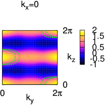
Figure 8: The singlet gap functions $d_{d}(\mbox{\boldmath$k$})$ in $k_{z}=\pi/2$ plane (left) and $k_{x}=0$ plane (right). The spin-flip scattering processes are fully taken into account. The broken curves represent the Fermi surface.

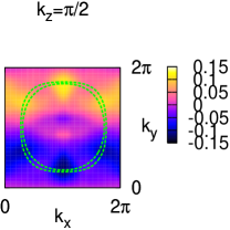
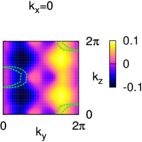
Figure 9: The triplet gap functions $d_{1}(\mbox{\boldmath$k$})$ in $k_{z}=\pi/2$ plane (left) and $k_{x}=0$ plane (right). The spin-flip scattering processes are fully taken into account. The broken curves represent the Fermi surface.

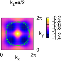
Figure 10: The singlet gap functions $d_{0}(\mbox{\boldmath$k$})$ in $k_{z}=\pi/2$ plane (left) and $k_{x}=0$ plane (right). The spin-flip scattering processes are not taken into account. The broken curves represent the Fermi surface.

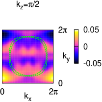
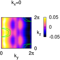
Figure 11: The triplet gap functions $d_{1}(\mbox{\boldmath$k$})$ in $k_{z}=\pi/2$ plane (left) and $k_{x}=0$ plane (right). The spin-flip scattering processes are not taken into account. The broken curves represent the Fermi surface.

In both cases, the singlet gap function is approximately $d_{0}(\mbox{\boldmath$k$})\sim\cos(2k_{z}a)$. The ratio of the triplet gap function to the singlet gap function defined as $r\equiv|{\rm max}\{d_{1}(\mbox{\boldmath$k$})\}|/|{\rm max}\{d_{0}(\mbox{\boldmath$k$})\}|$ is about $r\sim 1/10$ for case (i) and $r\sim 1/30$ for case (ii). Although $r$ is enhanced by the spin-flip processes, it still remains small in our system. We have performed similar calculations for various Fermi surfaces, and found that, generally, the spin-flip processes can enhance $r$. However, the value of $r$ depends on the details of the system. In CeRhSi₃ and CeIrSi₃, we conclude that the admixture of the gap functions is small. Therefore, the results in Sec.IV where we have neglected the spin-flip processes in the pairing interaction are supported. Finally, we note that the $k$-dependence of the triplet gap function is largely affected by the spin-flip processes. If we write $\tilde{V}=\tilde{V}_{\rm con}+c\tilde{V}_{\rm flip}$ with a tuning parameter $c$, the change in $d_{\mu}$ with respect to $c$ is continuous, although $d_{1}$ for case (i) and (ii) look quite different from each other. This difference in the $k$-dependence in $d_{1}$ is not important for the discussion of $H_{c2}$ in Sec.IV.

V.2 field dependence of spin fluctuations

The field dependence of the spin fluctuations is another effect which has been neglected in Sec.IV. Experimentally observed $H_{c2}$ is so large especially for $H_{c2}\parallel\hat{z}$ that one might think that the susceptibility $\hat{\chi}(q)$ is affected by the applied field and the spin fluctuations are weakened. We show, however, that the effect of the applied field on $\hat{\chi}(q)$ is strongly suppressed by the Rashba SO interaction. This is because the Rashba SO coupling tends to fix the direction of the spins on the Fermi surface depending on $k$-vectors, which competes with the Zeeman effect. As a result, the spin fluctuations in CeRhSi₃ and CeIrSi₃ are robust against the applied magnetic field up to the strength of the Rashba SO interaction, $\mu_{B}H\lesssim\alpha$.

We compute $\hat{\chi}(q)$ under finite fields $\mbox{\boldmath$H$}=(0,H_{y},0)$ or $(0,0,H_{z})$,

$$\begin{split}\chi_{\mu\nu}(q)&=\int_{0}^{1/T}d\tau e^{i\nu_{n}\tau}\langle TS^{\mu}_{q}(\tau)S^{\nu}_{-q}(0)\rangle\\ &=\frac{1}{4}\sigma^{\mu}_{\alpha\beta}\chi_{\alpha\beta\beta^{\prime}\alpha^{\prime}}(q)\sigma^{\nu}_{\alpha^{\prime}\beta^{\prime}}\end{split}$$ (86)

where $\chi_{\alpha\beta\beta^{\prime}\alpha^{\prime}}(q)$ is evaluated within RPA used in Sec.V.1. We fix $U$ and $T$, as in the previous section, $U=3.5t_{1}$ and $T=0.02t_{1}$. In Fig.12, $H$-dependence of $\chi_{xx},\chi_{yy}$ and $\chi_{zz}$ is shown for $\mbox{\boldmath$H$}=(0,0,H_{z})$.

Figure 12: Perpendicular filed $h_{z}=\mu_{B}H_{z}/t_{1}$ dependence of the susceptibility $\chi_{\mu\nu}(i\nu_{n}=0,\mbox{\boldmath$q$})$ at $q_{z}=\pi/2$ for $U=3.5t_{1}$ and $T=0.02t_{1}$. The strength of the Rashba SO interaction is $\alpha=0.2t_{1}$. $\chi_{xx}$(left), $\chi_{yy}$(center), and $\chi_{zz}$(right).

At $H=0$, $\chi_{xx}(0,\mbox{\boldmath$Q$}_{x})=\chi_{yy}(0,\mbox{\boldmath$Q$}_{y})>\chi_{zz}(0,\mbox{\boldmath$Q$}_{x,y})$ are satisfied, which is consistent with the result of the neutron scattering experiments in CeRhSi₃ that the antiferromagnetic moment is in $ab$-plane. pap:Aso Here, $\mbox{\boldmath$Q$}_{x}\sim(\pm 0.5\pi,0,0.5\pi)$ and $\mbox{\boldmath$Q$}_{y}\sim(0,\pm 0.5\pi,0.5\pi)$. Note that $\chi_{xx}(0,\mbox{\boldmath$Q$}_{x})>\chi_{yy}(0,\mbox{\boldmath$Q$}_{x})$ is satisfied because of the spin-flip scattering processes. However, the anisotropy in the non-interacting $\chi^{0}_{\mu\mu}(q)$ is of the order of $\alpha/\varepsilon_{F}\ll 1$, and therefore, the anisotropy in $\chi_{\mu\mu}(q)$ including the electron correlation effect remains irrelevant for the discussion of $H_{c2}$ even near the QCP. As mentioned above, for $\mu_{B}H\lesssim\alpha$, $\{\chi_{\mu\mu}\}$ are almost unchanged. For $\mu_{B}H\gtrsim\alpha$, only $\chi_{zz}$ is suppressed. The robustness of $\{\chi_{\mu\mu}\}$ for $\mu_{B}H\lesssim\alpha$ is a general feature of the noncentrosymmetric systems, since the spins for every $k$-point are fixed by the anisotropic SO interaction in that region. These calculated results support the legitimacy of our neglecting the field dependence of the pairing interaction for the calculation of $H_{c2}$. Although there is no direct observation of the strength of the SO interaction, it is expected to be pretty large, $\alpha>\mu_{B}H_{c2}\sim 30\mu_{B}$(K). Therefore, in CeRhSi₃ and CeIrSi₃, the spin fluctuations remain so strong under applied magnetic fields that $H_{c2}$ is strongly enhanced.

The same robustness also exists for $\mbox{\boldmath$H$}=(0,H_{y},0)$ for which the Fermi surface is distorted anisotropically. Figure13 shows the field dependence of $\chi_{\mu\mu}$. All of $\chi_{\mu\mu}$ are almost unchanged for $\mu_{B}H\lesssim\alpha$, and $\chi_{yy}$ is suppressed for $\mu_{B}H\gtrsim\alpha$.

Figure 13: In-plane filed $h_{y}=\mu_{B}H_{y}/t_{1}$ dependence of the susceptibility $\chi_{\mu\nu}(0,\mbox{\boldmath$q$})$ at $k_{z}=\pi/2$ for $U=3.5t_{1}$ and $T=0.02t_{1}$. The strength of the Rashba SO interaction is $\alpha=0.2t_{1}$. $\chi_{xx}$(left), $\chi_{yy}$(center), and $\chi_{zz}$(right).

These behaviors are basically the same as those for $\mbox{\boldmath$H$}\parallel\hat{z}$, and assert the robustness of the spin fluctuations against the in-plane field.

From the above results, we see that neglecting the field dependence in the pairing interaction for any field direction is legitimate provided $\mu_{B}H_{c2}\lesssim\alpha$. Although $H_{c2}$ is huge in CeRhSi₃ and CeIrSi₃ especially for $c$-axis, the condition $\mu_{B}H_{c2}\lesssim\alpha$ is expected to be satisfied. Therefore, the discussion of $H_{c2}$ in Sec.IV is not changed even if we consider the field dependence of the spin fluctuations.

VI Summary

We have discussed the normal and the superconducting properties in noncentrosymmetric heavy fermion superconductors CeRhSi₃ and CeIrSi₃. We have shown that the $T$-linear dependence of the resistivity above $T_{c}$ observed experimentally is naturally understood within the 3D spin fluctuations near the AF QCP.

For the superconducting state, we have derived a formula from the Eliashberg equation in real space. The formula enables us to treat the Pauli and the orbital depairing effects on an equal footing. Furthermore, by using it, we can calculate $H_{c2}$ for strong coupling superconductors with general Fermi surfaces. We have calculated $H_{c2}$ with the formula and have well explained the observed features of $H_{c2}$ in CeRhSi₃ and CeIrSi₃. For $H\parallel\hat{z}$, $H_{\rm P}$ is infinitely large due to the Rashba SO interaction, and $H_{c2}$ is determined by $H_{\rm orb}$. As temperature is lowered and the system approaches the QCP, the pairing interaction becomes larger while the quasiparticle life time becomes longer, which results in the huge $H_{\rm orb}\simeq H_{c2}$ with the strong pressure dependence. The enhancement of the orbital limiting field near QCPs by this mechanism would be universal. We have also discussed the case for $H\perp\hat{z}$. In this case, the Pauli depairing effect is significant because of the asymmetric distortion of the Fermi surface, and resulting $H_{c2}$ is moderate against the pressure. The FFLO state can be stabilized for a large $H$ region, although such a region is very small. The features of the calculated $H_{c2}$ for both $H\parallel\hat{z}$ and $H\perp\hat{z}$ are in good agreement with the experiments. This consistency supports the scenario that the superconductivity in CeRhSi₃ and CeIrSi₃ is mediated by the spin fluctuations near the AF QCP.

In the last section, we have checked the legitimacy of our approximation used for the calculation of $H_{c2}$. In CeRhSi₃ and CeIrSi₃, the admixture of the singlet and the triplet gap functions are small even if we take into account the spin-flip scattering processes in the pairing interaction. In noncentrosymmetric systems, the spin susceptibility is robust against the applied magnetic fields $\mu_{B}H\lesssim\alpha$. For this reason, the spin fluctuations near the AF QCP in CeRhSi₃ and CeIrSi₃ remain strong even under a large magnetic field $\sim 30$ (T). Therefore, the above mentioned results for $H_{c2}$ is not changed if we refine our approximation used in the calculation of $H_{c2}$.

References

- (1) V. M. Edelstein, Sov. Phys. JETP 68, 1244 (1989).
- (2) V. M. Edelstein, Phys. Rev. Lett. 75, 2004 (1995).
- (3) S. K. Yip, Phys. Rev. B 65, 144508 (2002).
- (4) L. P. Gor’kov and E. Rashba, Phys. Lett. 87, 037004 (2001).
- (5) P. A. Frigeri, D. F. Agterberg, A. Koga, and M. Sigrist, Phys. Rev. Lett. 92, 097001 (2004).
- (6) K. V. Samokhin, E. S. Zijlstra, and S. K. Bose, Phys. Rev. B 69, 094514 (2004); Phys. Rev. B 70, 069902(E) (2004).
- (7) K. V. Samokhin, Phys. Rev. Lett. 94, 027004 (2005).
- (8) V. P. Mineev, Phys. Rev. B 71, 012509 (2005).
- (9) V. P. Mineev and K. V. Samokhin, Phys. Rev. B 75, 184529 (2007).
- (10) S. Fujimoto, Phys. Rev. B 72, 024515 (2005).
- (11) S. Fujimoto, J. Phys. Soc. Jpn. 76, 034712 (2007).
- (12) S. Fujimoto, J. Phys. Soc. Jpn. 76, 051008 (2007).
- (13) N. Kimura, K. Ito, K. Saitoh, Y. Umeda, H. Aoki, and T. Terashima, Phys. Rev. Lett. 95, 247004 (2005).
- (14) Y. Muro, M. Ishikawa, K. Hirota, Z. Hiroi, N. Takeda, N. Kimura, and H. Aoki, J. Phys. Soc. Jpn. 76, 033706 (2007).
- (15) N. Kimura, Y. Muro, and H. Aoki, J. Phys. Soc. Jpn. 76, 051010 (2007).
- (16) I. Sugitani, Y. Okuda, H. Shishido, T. Yamada, A. Thamizhavel, E. Yamamoto, T. D. Matsuda, Y. Haga, T. Takeuchi, R. Settai, and Y. Ōnuki, J. Phys. Soc. Jpn. 75, 043703 (2006).
- (17) Y. Okuda, Y. Miyauchi, Y. Ida, Y. Takeda, C. Tonohiro, Y. Oduchi, T. Yamada, N. D. Dung, T. D. Matsuda, Y. Haga, T. Takeuchi, M. Hagiwara, K. Kindo, H. Harima, K. Sugiyama, R. Settai, and Y. Ōnuki, J. Phys. Soc. Jpn. 76, 044708 (2007).
- (18) N. Aso, H. Miyano, H. Yoshizawa, N. Kimura, T. Komatsubara, and H. Aoki, J. Mag. Mag. Matt. 310, 602 (2007).
- (19) E. Bauer, G. Hilscher, H. Michor, Ch. Paul, E. W. Scheidt, A. Gribanov, Yu. Seropegin, H. Noël, M. Sigrist, and P. Rogl, Phys. Rev. Lett. 92, 027003 (2004).
- (20) H. Mukuda, T. Fujii, T. Ohara, A. Harada, M. Yashima, Y. Kitaoka, Y. Okuda, R. Settai, and Y. Ōnuki, Phys. Rev. Lett. 100, 107003 (2008).
- (21) T. Moriya and K. Ueda, Adv. Phys. 49, 555 (2000).
- (22) T. Moriya and K. Ueda, Rep. Prog. Phys. 66, 1299 (2003).
- (23) N. Tateiwa, Y. Haga, T. D. Matsuda, S. Ikeda, E. Yamamoto, Y. Okuda, Y. Miyauchi R. Settai, and Y. Ōnuki, J. Phys. Soc. Jpn. 76, 083706 (2007).
- (24) N. Kimura, K. Ito, H. Aoki, S. Uji, and T. Terashima, Phys. Rev. Lett. 98, 197001 (2007).
- (25) R. Settai, Y. Miyauchi, T. Takeuchi, F. Lévy, I. Siieikin, and Y. Ōnuki, J. Phys. Soc. Jpn. 74, 073705 (2008).
- (26) Y. Tada, N. Kawakami, and S. Fujimoto, Phys. Rev. Lett. 101, 267006 (2008).
- (27) R. P. Kaur, D. F. Agterberg, and M. Sigrist, Phys. Rev. Lett. 94, 137002 (2005).
- (28) Y. Yanase and M. Sigrist, J. Phys. Soc. Jpn. 76, 124709 (2007).
- (29) O. Dimitrova and M. V. Feigel’man, Phys. Rev. B 76, 014522 (2007).
- (30) D. F. Agterberg and R. P. Kaur, Phys. Rev. B 75, 064511 (2007).
- (31) K. V. Samokhin, Phys. Rev. B 78, 224520 (2008).
- (32) Y. Matsunaga, N. Hiasa, and R. Ikeda, Phys. Rev. B 78, 220508(R) (2008).
- (33) N. Hiasa, T. Saiki, and R. Ikeda, Phys. Rev. B 80, 014501 (2009).
- (34) V. P. Mineev and M. Sigrist, cond. mat. 0904.2962.
- (35) P. Fulde and R. A. Ferrell, Phys. Rev. 135, A550 (1964).
- (36) A. I. Larkin and Yu. N. Ovchinnikov, Sov. Phys. JETP 20, 762 (1965).
- (37) Y. Yanase and M. Sigrist, J. Phys. Soc. Jpn. 77, 124711 (2008).
- (38) T. Takimoto and P. Thalmeier, J. Phys. Soc. Jpn. 78, 103703 (2009).
- (39) A. Rosch, Phys. Rev. Lett. 82, 4280 (1999).
- (40) A. Rosch, Phys. Rev. B 62, 4945 (2000).
- (41) S. Onari, H. Kontani, and Y. Tanaka, Phys. Rev. B 73, 224434 (2006).
- (42) Y. Muro, D. Eom, N. Tanaka, and M. Ishikawa, J. Phys. Soc. Jpn. 67, 3601 (1998).
- (43) Y. Tada, N. Kawakami, and S. Fujimoto, J. Phys. Soc. Jpn. 77, 054707 (2008).
- (44) T. Terashima, M. Kimata, S. Uji, T. Sugawara, N. Kimura, H. Aoki, and H. Harima, Phys. Rev. B 78, 205107 (2008)
- (45) P. Monthoux and D. Pines, Phys. Rev. Lett. 69, 961 (1992).
- (46) P. Monthoux and G. G. Lonzarich, Phys. Rev. B 59, 14598 (1999).
- (47) K. Yonemitsu, J. Phys. Soc. Jpn. 58, 4576 (1989).
- (48) P. Monthoux, Phys. Rev. B 55, 15261 (1997).
- (49) G. M. Eliashberg, Sov. Phys. JETP 14, 886 (1962).
- (50) K. Yamada and K. Yoshida, Prog. Theor. Phys. 76, 621 (1986).
- (51) H. Kontani, K. Kanki, and K. Ueda, Phys. Rev. B 59, 14723 (1999).
- (52) K. Yamada, Electron Correlation in Metals, Cambridge university Press (2004).
- (53) B. P. Stojkovic and D. Pines, Phys. Rev. B 55, 8576 (1997).
- (54) N. R. Werthamer, E. Helfand, and P. C. Hohenberg, Phys. Rev. 147, 295 (1965).
- (55) M. Schossmann and E. Schachinger, Phys. Rev. B 33, 6123 (1986).
- (56) L. N. Bulaevskii, O. V. Dolgov, and M. O. Ptitsyn, Phys. Rev. B 38, 11290 (1988).
- (57) J. A. Hertz, Phys. Rev. B 14, 1165 (1976).
- (58) A. J. Millis, Phys. Rev. B 48, 7183 (1993).
- (59) N. T. Huy, A. Gasparini, D. E. de Nijs, Y. Huang, J. C. P. Klaasse, T. Gortenmulder, A. de Visser, A. Hamann, T. Görlach, and H. v. Löhneysen, Phys. Rev. Lett. 99, 067006 (2007).
- (60) E. Slooten, T. Naka, A. Gasparini, Y. K. Huang, and A. de Visser, Phys. Rev. Lett. 103, 097003 (2009).
- (61) D. Aoki, T. D. Matsuda, V. Taufour, E. Hassinger, G. Knebel, and J. Flouquet, J. Phys. Soc. Jpn. 78, 113709 (2009).