A nonlinear theory of the parallel firehose and gyrothermal instabilities in a weakly collisional plasma

Abstract

Weakly collisional magnetized cosmic plasmas have a dynamical tendency to develop pressure anisotropies with respect to the local direction of the magnetic field. These anisotropies trigger plasma instabilities at scales just above the ion Larmor radius $\rho_{i}$ and much below the mean free path $\lambda_{\mathrm{mfp}}$. They have growth rates of a fraction of the ion cyclotron frequency, which is much faster than either the global dynamics or even local turbulence. Despite their microscopic nature, these instabilities dramatically modify the transport properties and, therefore, the macroscopic dynamics of the plasma. The nonlinear evolution of these instabilities is expected to drive pressure anisotropies towards marginal stability values, controlled by the plasma beta $\beta_{i}$. Here this nonlinear evolution is worked out in an ab initio kinetic calculation for the simplest analytically tractable example — the parallel ($k_{\perp}=0$) firehose instability in a high-beta plasma. An asymptotic theory is constructed, based on a particular physical ordering and leading to a closed nonlinear equation for the firehose turbulence. In the nonlinear regime, both analytical theory and the numerical solution predict secular ($\propto t$) growth of magnetic fluctuations. The fluctuations develop a $k_{\parallel}^{-3}$ spectrum, extending from scales somewhat larger than $\rho_{i}$ to the maximum scale that grows secularly with time ($\propto t^{1/2}$); the relative pressure anisotropy $(p_{\perp}-p_{\parallel})/p_{\parallel}$ tends to the marginal value $-2/\beta_{i}$. The marginal state is achieved via changes in the the magnetic field, not particle scattering. When a parallel ion heat flux is present, the parallel firehose mutates into the new gyrothermal instability (GTI), which continues to exist up to firehose-stable values of pressure anisotropy, which can be positive and are limited by the magnitude of the ion heat flux. The nonlinear evolution of the GTI also features secular growth of magnetic fluctuations, but the fluctuation spectrum is eventually dominated by modes around a maximal scale $\sim\rho_{i}l_{T}/\lambda_{\mathrm{mfp}}$, where $l_{T}$ is the scale of the parallel temperature variation. Implications for momentum and heat transport are speculated about. This study is motivated by our interest in the dynamics of galaxy cluster plasmas (which are used as the main astrophysical example), but its relevance to solar wind and accretion flow plasmas is also briefly discussed.

1 Introduction

It has recently been realized in various astrophysics and space physics contexts that pressure anisotropies (with respect to the direction of the magnetic field) occur naturally and ubiquitously in magnetized weakly collisional plasmas. They lead to very fast microscale instabilities, firehose, mirror, and others, whose presence is likely to fundamentally affect the transport properties and, therefore, both small- and large-scale dynamics of astrophysical plasmas — most interestingly, the plasmas of galaxy clusters and accretion discs (Hall & Sciama, 1979; Schekochihin & Cowley, 2006; Schekochihin et al., 2005, 2008; Sharma et al., 2006, 2007; Lyutikov, 2007). These instabilities occur even (and especially) in high-beta plasmas and even when the magnetic field is dynamically weak. The current state of theoretical understanding of this problem is such that we do not even have a set of well-posed macroscopic equations that govern the dynamics of a plasma in which the collisional mean free path exceeds the ion Larmor radius, $\lambda_{\mathrm{mfp}}\gg\rho_{i}$ (equivalently, ion collision frequency is smaller than the ion cyclotron frequency, $\nu_{ii}\ll\Omega_{i}$). This is because calculating the dynamics at long spatial scales $l\gg\rho_{i}$ and slow time scales corresponding to frequencies $\omega\ll\Omega_{i}$ requires knowledge of the form of the pressure tensor and the heat fluxes, which depend on the nonlinear evolution and saturation of the instabilities triggered by the pressure anisotropies and temperature gradients. Since this is not currently understood, we do not have an effective mean-field theory for the large-scale dynamics.

In the absence of a microphysical theory, it is probably sensible to assume that the instabilities will return the pressure anisotropies to the marginal level and to model large-scale dynamics on this basis, via a suitable closure scheme (Sharma et al., 2006, 2007; Schekochihin & Cowley, 2006; Lyutikov, 2007; Kunz et al., 2011). This approach appears to be supported by the solar wind data (Gary et al., 2001; Kasper, Lazarus & Gary, 2002; Marsch, Ao & Tu, 2004; Hellinger et al., 2006; Matteini et al., 2007; Bale et al., 2009). However, a first-principles calculation of the nonlinear evolution of the instabilities remains a theoretical imperative because, in order to construct the correct closure, we must understand the mechanism whereby the instabilities control the pressure anisotropy: do they scatter particles? do they modify the structure of the magnetic field? The calculation presented below will lead us to conclude that the latter mechanism is at work, at least in the simple case we are considering (see discussion in section 6.1), and indeed a sea of microscale magnetic fluctuations excited by the plasma instabilities will act to pin the plasma to marginal stability.

In this paper, we present a theory of the nonlinear evolution of the simplest of the pressure-anisotropy-driven instabilities, the parallel ($k_{\perp}=0$) firehose instability and the gyrothermal instability (Schekochihin et al., 2010). To be specific, we consider as our main application a plasma under physical conditions characteristic of galaxy clusters: weakly collisional, fully ionized, magnetized and approximately (locally) homogeneous. We will explain at the end the extent to which our results are likely to be useful in other contexts, e.g., accretion flows and the solar wind (section 7).

The plan of exposition is as follows. In section 2, we give an extended, qualitative, mostly low-analytical-intensity introduction to the problem, explain the relevant properties of the intracluster plasma (section 2.1), the origin of the pressure anisotropies (section 2.2), sketch the linear theory of the firehose instability (section 2.3), the main principle of its nonlinear evolution (section 2.4), and show that a more complicated theory is necessary to work out the spatial structure of the resulting “firehose turbulence” (section 2.5). In section 3, a systematic such theory is developed via asymptotic expansions of the electron and ion kinetics (the basic structure of the theory is outlined in the main part of the paper, while the detailed derivation is relegated to Appendix A), culminating in a very simple one-dimensional equation for the nonlinear evolution of the firehose fluctuations (section 4.1), the study of which is undertaken in section 4. The results are a theoretical prediction for the nonlinear evolution and spectrum of the firehose turbulence (section 4.3) and some tentative conclusions about its effect on the momentum transport (section 4.4). In section 5, we extend this study to include the effect of parallel ion heat flux on the firehose turbulence: in the presence of a parallel ion temperature gradient, a new instability emerges (the gyrothermal instablity recently reported by Schekochihin et al. 2010 and recapitulated in section 5.2) — which, under some conditions, can take over from the firehose. For it as well, we develop a one-dimensional nonlinear equation (section 5.1), solve it to predict the nonlinear evolution and spatial structure of the gyrothermal turbulence (section 5.3) and discuss the implications for momentum transport (section 5.4). A discussion of our results and of the ways in which they differ from previous work on firehose instability in collisionless plasmas is given in section 6. A brief survey of astrophysical implications (both galaxy clusters and other contexts) follows in section 7. Finally, section 8 contains a very concise summary of our findings and of the outlook for future work. Note that while section 2 is largely a pedagogical review of our earlier work (Schekochihin & Cowley, 2006; Schekochihin et al., 2005, 2008), most of the theory and results presented in sections 3–5 is new.

A reader not interested in the technicalities of kinetic theory is advised to ignore section 3 and Appendix A. A reader only interested in the formal derivation may skip section 2, as section 3 (supplemented by Appendix A) and the sections that follow it can be read in a self-contained way.

2 Qualitative considerations

2.1 Galaxy clusters: observations, questions, parameters

Galaxy clusters have long attracted the interest of both theoreticians and observers both as dynamical systems in their own right and as cosmological probes (Bahcall, 2000; Peterson & Fabian, 2006). While gravitationally they are dominated by dark matter, most of their luminous matter is a hot, diffuse, fully ionized, X-ray emitting hydrogen plasma (Sarazin, 2003) known as the intracluster medium, or ICM (the galaxies themselves are negligible both in terms of their mass and the volume they occupy). Crudely, we can think of an observable galaxy cluster as an amorphous blob of ICM about $1$ Mpc across, sitting in a gravitational well, with a density profile peaking at the center and decaying outwards. Observationally, on the crudest level, we know what the overall density and temperature profiles in clusters are (e.g., Vikhlinin et al., 2005; Piffaretti et al., 2005; Leccardi & Molendi, 2008; Cavagnolo et al., 2009). Recent highly resolved X-ray observations reveal the ICM to be a rich, complicated, multiscale structure displaying ripples, bubbles, filaments, waves, shocks, edges etc. (Fabian et al., 2003a, b, 2005a, 2006; Sanders & Fabian, 2006, 2008; Forman et al., 2007; Markevitch & Vikhlnin, 2007), temperature fluctuations (Simionescu et al., 2001; Markevitch et al., 2003; Fabian et al., 2006; Million & Allen, 2009; Sanders et al., 2010a; Laganá, Andrade-Santos & Lima Neto, 2010) and most probably also broad-band disordered turbulent motions (Churazov et al., 2004; Schuecker et al., 2004; Rebusco et al., 2005, 2006, 2008; Graham et al., 2006; Sanders et al., 2010b, 2011; Ogrean et al., 2010). Radio observations tell us that the ICM also hosts tangled magnetic fields, which are probably dynamically strong (Carilli & Taylor, 2002; Govoni & Feretti, 2004; Vogt & Enßlin, 2005; Kuchar & Enßlin, 2009; Clarke & Enßlin, 2006; Govoni et al., 2006; Guidetti et al., 2008; Ferrari et al., 2008).

These and other observations motivate a number of questions about the ICM, which are representative of the problems generally posed for astrophysical plasma systems:

• Can we explain the observed ICM temperature profiles, in particular the apparent lack of a cooling catastrophe at the cluster core predicted by fluid models (Fabian, 1994; Binney, 2003; Peterson & Fabian, 2006; Parrish, Quataert & Sharma, 2009; Bogdanović et al., 2009)? This requires modelling various heating processes involving conversion of the energy of plasma motions (turbulent or otherwise) into heat via some form of effective viscosity (e.g., Omma et al., 2004; Fabian et al., 2005b; Dennis & Chandran, 2005; Chandran & Rasera, 2007; Guo, Oh & Ruszkowski, 2008; Brüggen & Scannapieco, 2009; Kunz et al., 2011), the dynamical effect of thermal instabilities arising in the magnetized ICM (Balbus, 2000; Parrish, Stone & Lemaster, 2008; Quataert, 2008; Sharma, Quataert & Stone, 2008; Sharma et al., 2009; Parrish, Quataert & Sharma, 2009, 2010; Bogdanović et al., 2009; Ruszkowski & Oh, 2010; Schekochihin et al., 2010), and the effective thermal conductivity of this medium with account taken of the tangled magnetic field (Chandran & Cowley, 1998; Malyshkin, 2001; Narayan & Medvedev, 2001; Zakamska & Narayan, 2003; Cho et al., 2003; Voigt & Fabian, 2004).

• Can we construct theoretical and numerical models of the ICM dynamics that reproduce quantitatively the features we observe, e.g., the rise of radio bubbles (e.g., Ruszkowski et al., 2007; Dong & Stone, 2009), the formation and propagation of shocks, fronts and sound waves, the structure of ICM velocity, density, temperature fluctuations?

• Can we explain the origin of the cluster magnetic fields (probably via some form of turbulent dynamo, see Subramanian, Shukurov & Haugen 2006; Schekochihin & Cowley 2006; Enßlin & Vogt 2006; Xu et al. 2009) and their observed spatial structure?

Addressing these questions requires a theoretically sound mean-field theory for the ICM dynamics, i.e., a set of prescriptions for its effective transport properties (viscosity, thermal conductivity), which depend on the unresolved microphysics. Without such a theory, all we have is numerical simulations based on fluid models (see references above), which, while they can often be tuned to produce results that are visually similar to what is observed, are not entirely satisfactory because they lack a solid plasma-physical basis and because refining the numerical resolution often breaks the agreement with observations and requires retuning. A satisfactory transport theory is lacking because any plasma motions in the ICM that change the strength of the magnetic field trigger microscale plasma instabilities (see sections 2.2 and 2.3) and we do not know what happens next.

How some of these instabilities arise and evolve is discussed in greater detail below. In order to make this discussion more quantitative, we need to fix a few physical parameters that characterize the ICM. In reality, these parameters vary considerably both between different clusters and within any individual cluster (as a function of radius: from the cooler, denser core to the hotter, more diffuse outer regions). However, for the purposes of this discussion, it is sufficient to adopt a set of fiducial values. Let us consider the plasma in the core of the Hydra A cluster (also used as a representative example in our preceding papers, Schekochihin & Cowley 2006; Schekochihin et al. 2008), where the parameters are (David et al., 2001; Enßlin & Vogt, 2006)

• particle (ion and electron) number density

  $$n_{i}=n_{e}\sim 6\times 10^{-2}~{}\mathrm{cm}^{-3};$$ (1)

• measured electron temperature is

  $$T_{e}\sim 3\times 10^{7}~{}\mathrm{K};$$ (2)

  the ion temperature is unknown, but assumed to be comparable, $T_{i}\sim T_{e}$; then the ion thermal speed is

  $$v_{\mathrm{th}i}=\left(\frac{2T_{i}}{m_{i}}\right)^{1/2}\sim 7\times 10^{7}~{}\mathrm{cm~{}s}^{-1}$$ (3)

  ($m_{i}$ is the ion mass, $T_{i}$ is in erg); the ion Debye length is

  $$\lambda_{Di}=\frac{v_{\mathrm{th}i}}{\omega_{pi}}=v_{\mathrm{th}i}\left(\frac{4\pi e^{2}n_{i}}{m_{i}}\right)^{-1/2}\sim 2\times 10^{5}~{}\mathrm{cm};$$ (4)

• the ion-ion collision frequency (in seconds, assuming $n_{i}$ in cm^-3 and $T_{i}$ in K) is

  $$\nu_{ii}\sim 1.5n_{i}T_{i}^{-3/2}\sim 5\times 10^{-13}~{}\mathrm{s}^{-1};$$ (5)

  consequently the mean free path is

  $$\lambda_{\mathrm{mfp}}=\frac{v_{\mathrm{th}i}}{\nu_{ii}}\sim 1.3\times 10^{20}~{}\mathrm{cm};$$ (6)

• the rms magnetic field strength is (Vogt & Enßlin, 2005)

  $$B\sim 7\times 10^{-6}~{}\mathrm{G};$$ (7)

  consequently the plasma (ion) beta is

  $$\beta_{i}=\frac{8\pi n_{i}T_{i}}{B^{2}}\sim 130,$$ (8)

  the ion cyclotron frequency is

  $$\Omega_{i}=\frac{eB}{m_{i}c}\sim 0.07~{}\mathrm{s}^{-1}$$ (9)

  ($e$ is the elementary charge, $c$ the speed of light) and the ion Larmor radius is

  $$\rho_{i}=\frac{v_{\mathrm{th}i}}{\Omega_{i}}\sim 10^{9}~{}\mathrm{cm};$$ (10)

  note that the magnetized-plasma condition $\rho_{i}\ll\lambda_{\mathrm{mfp}}$ is satisfied extremely well;

• the typical velocity of the plasma motions is

  $$U\sim 2.5\times 10^{7}~{}\mathrm{cm~{}s}^{-1}$$ (11)

  (cf. Sanders et al., 2010b, 2011, who consider a sample of clusters), while the typical length scale of these motions is

  $$L\sim 2\times 10^{22}~{}\mathrm{cm};$$ (12)

  consequently the Mach number is

  $$M=\frac{U}{v_{\mathrm{th}i}}\sim 0.3$$ (13)

  (so the motions are subsonic, hence approximately incompressible on scales smaller than that of the mean density variation) and the Reynolds number based on collisional parallel viscosity is

  $$\mathrm{Re}=\frac{LU}{\lambda_{\mathrm{mfp}}v_{\mathrm{th}i}}\sim 60,$$ (14)

  assuming Kolmogorov scalings for turbulence, the viscous cutoff scale is

  $$l\sim L\mathrm{Re}^{-3/4}\sim 10^{21}~{}\mathrm{cm}$$ (15)

  and the typical velocity at this scale is

  $$u\sim U\mathrm{Re}^{-1/4}\sim 10^{7}~{}\mathrm{cm~{}s}^{-1},$$ (16)

  so the approximate rms rate of strain (assuming a viscous cutoff for the motions) is

  $$\gamma_{0}\sim\frac{u}{l}\sim\frac{U}{L}\,\mathrm{Re}^{1/2}\sim 10^{-14}~{}\mathrm{s}^{-1}.$$ (17)

2.2 Origin of pressure anisotropy

If we consider length scales greater than $\rho_{i}$ and time scales longer than $\Omega_{i}$ (which is easily true for any large-scale dynamical processes in the ICM), the momentum equation for the plasma flow, characterized by the mean velocity $\mn@boldsymbol{u}$, is (e.g., Kulsrud, 1983)

$$m_{i}n_{i}\frac{\mathrm{d}\mn@boldsymbol{u}}{\mathrm{d}t} = -\mn@boldsymbol{\nabla}\left(p_{\perp}+\frac{B^{2}}{8\pi}\right)$$ (18)

$$+\,\,\mn@boldsymbol{\nabla}\cdot\left[\mn@boldsymbol{\hat{b}}\mn@boldsymbol{\hat{b}}\left(p_{\perp}-p_{\parallel}+\frac{B^{2}}{4\pi}\right)\right],$$

where ${\mathrm{d}\mn@boldsymbol{u}}/{\mathrm{d}t}=\partial/\partial t+\mn@boldsymbol{u}\cdot\mn@boldsymbol{\nabla}$ is the convective derivative, $\mn@boldsymbol{\hat{b}}$ is the unit vector in the direction of the local magnetic field, $B$ is the field’s strength, and $p_{\perp}$ and $p_{\parallel}$ are the perpendicular and parallel plasma pressure, which are the only components of the plasma pressure tensor that survive at these long spatial and temporal scales:

$$\textbf{{P}}=\sum_{s}m_{s}\int\mathrm{d}^{3}\mn@boldsymbol{v}\,\mn@boldsymbol{v}\mn@boldsymbol{v}\,f_{s} = p_{\perp}\left(\textbf{{I}}-\mn@boldsymbol{\hat{b}}\mn@boldsymbol{\hat{b}}\right)+p_{\parallel}\mn@boldsymbol{\hat{b}}\mn@boldsymbol{\hat{b}},$$ (19)

$$p_{\perp} = \sum_{s}m_{s}\int\mathrm{d}^{3}\mn@boldsymbol{v}\,\frac{v_{\perp}^{2}}{2}\,f_{s},$$ (20)

$$p_{\parallel} = \sum_{s}m_{s}\int\mathrm{d}^{3}\mn@boldsymbol{v}\,v_{\parallel}^{2}f_{s},$$ (21)

where $f_{s}$ is the distribution function for species $s$ ($s=i,e$), $\mn@boldsymbol{v}$ its velocity variable (particle’s peculiar velocity), and $v_{\perp}$ and $v_{\parallel}$ the projections of $\mn@boldsymbol{v}$ perpendicular and parallel to the magnetic field. The magnetic field is determined by the combination of Faraday’s and Ohm’s laws, which at these long scales takes the form of the ideal induction equation

$$\frac{\mathrm{d}\mn@boldsymbol{B}}{\mathrm{d}t}=\mn@boldsymbol{B}\cdot\mn@boldsymbol{\nabla}\mn@boldsymbol{u}-\mn@boldsymbol{B}\mn@boldsymbol{\nabla}\cdot\mn@boldsymbol{u}.$$ (22)

Without as yet going into the technicalities of kinetic theory, it is not hard to show that pressure anisotropies arise naturally in a weakly collisional plasma. Indeed, the first adiabatic invariant $\mu=v_{\perp}^{2}/2B$ of a gyrating particle is conserved on time scales intermediate between the collision time and the cyclotron period (a nonempty interval when plasma is magnetized, $\nu_{ii}\ll\Omega_{i}$). Since $p_{\perp}$ is proportional to the sum of the values of $\mu$ for all particles, $p_{\perp}/B$ should be a conserved quantity, i.e., if the magnetic field changes (as a result of plasma motions into which the flux is frozen, see equation (22)) then $p_{\perp}$ should change accordingly. For the purposes of this qualitative discussion, we may momentarily ignore the fact that changing $B$ also causes $p_{\parallel}$ to change (in a different way from $p_{\perp}$; see Appendix A.2.15) and so conclude that changing $B$ will cause pressure anisotropies to develop.

In the absence of collisions, the pressure anisotropies would track the field strength. If collisions do occur, even weakly, their effect will be to relax the system towards an isotropic pressure (and a Maxwellian distribution). Thus, there is a competition between changing $B$ inducing anisotropy and collisions causing isotropization. This can be modelled by the following heuristic equation:

$$\frac{1}{p_{\perp}}\frac{\mathrm{d}p_{\perp}}{\mathrm{d}t} \sim \frac{1}{B}\frac{\mathrm{d}B}{\mathrm{d}t}-\nu_{ii}\frac{p_{\perp}-p_{\parallel}}{p_{\perp}}$$ (23)

$$= \mn@boldsymbol{\hat{b}}\mn@boldsymbol{\hat{b}}:\mn@boldsymbol{\nabla}\mn@boldsymbol{u}-\nu_{ii}\frac{p_{\perp}-p_{\parallel}}{p_{\perp}},$$

where we have used equation (22) to express the change in the field strength in terms of the plasma flow velocity and assumed, for the purposes of this qualitative discussion, that plasma density is constant (i.e., the motions are incompressible). Considering what happens on time scales longer than the collision time, we conclude, after examining the right-hand side of equation (23), that we should expect the typical (ion) pressure anisotropy in a moving plasma to be

$$\Delta=\frac{p_{\perp}-p_{\parallel}}{p_{\perp}}\sim\frac{1}{\nu_{ii}}\frac{1}{B}\frac{\mathrm{d}B}{\mathrm{d}t}\sim\frac{\gamma_{0}}{\nu_{ii}},$$ (24)

where $\gamma_{0}$ is the typical rate of strain of the plasma motion. Thus, the pressure anisotropy is regulated by the ratio of the typical rate of change of the magnetic-field strength to the collision frequency.

Substituting the numbers from section 2.1, we find that $|\Delta|\sim 0.02$ in the core of Hydra A. Is this a large number? It turns out that it is a huge number because such anisotropies will make the plasma motion violently unstable.

2.3 Firehose instability

While the full description of the plasma instabilities triggered by pressure anisotropies requires kinetic treatment, it is extremely straightforward to deduce the presence of the firehose instability directly from equation (18).

Consider some “fluid” solution $(\mn@boldsymbol{u}_{0},\mn@boldsymbol{B}_{0},p_{0\perp},p_{0\parallel})$ of equations (18) and (22) that varies on long time and spatial scales — that can be thought of as the turbulence and/or some regular magnetofluid motion caused by global dynamics. Let us now examine the linear stability of this solution with respect to high-frequency ($\omega\gg|\mn@boldsymbol{\nabla}\mn@boldsymbol{u}_{0}|$), short-scale ($k\gg|\mn@boldsymbol{\nabla}\mn@boldsymbol{u}_{0}|/u_{0}$) perturbations $(\delta\mn@boldsymbol{u},\delta\mn@boldsymbol{B},\delta p_{\perp},\delta p_{\parallel})$. Mathematically, this is simply equivalent to perturbing a straight-magnetic-field equilibrium of equations (18) and (22):

$$-m_{i}n_{i}\omega\delta\mn@boldsymbol{u} = -\mn@boldsymbol{k}_{\perp}\left(\delta p_{\perp}+\frac{B_{0}\delta B_{\parallel}}{4\pi}\right)$$ (25)

$$+\,\,k_{\parallel}\delta\mn@boldsymbol{\hat{b}}\left(p_{0\perp}-p_{0\parallel}+\frac{B_{0}^{2}}{4\pi}\right)$$

$$-\,\,k_{\parallel}\mn@boldsymbol{\hat{b}}_{0}\left[\delta p_{\parallel}+\left(p_{0\perp}-p_{0\parallel}\right)\frac{\delta B_{\parallel}}{B_{0}}\right],$$

$$-\omega\frac{\delta\mn@boldsymbol{B}}{B_{0}} = k_{\parallel}\delta\mn@boldsymbol{u}-\mn@boldsymbol{\hat{b}}_{0}\left(\mn@boldsymbol{k}\cdot\delta\mn@boldsymbol{u}\right),$$ (26)

where $\delta\mn@boldsymbol{\hat{b}}=\delta\mn@boldsymbol{B}_{\perp}/B_{0}$, we have used $\mn@boldsymbol{k}\cdot\delta\mn@boldsymbol{\hat{b}}=-k_{\parallel}\delta B_{\parallel}/B_{0}$ (from $\mn@boldsymbol{\nabla}\cdot\mn@boldsymbol{B}=0$), and $\perp$ and $\parallel$ are with respect to the unperturbed magnetic field direction $\mn@boldsymbol{\hat{b}}_{0}$. Pressure perturbations can only be calculated from the linearized kinetic equation (see, e.g., Schekochihin et al., 2005), but even without knowing them, we find that for the Alfvénically polarized modes, $\delta\mn@boldsymbol{u}\propto\mn@boldsymbol{\hat{b}}_{0}\times\mn@boldsymbol{k}$, the dispersion relation is

$$\omega=\pm k_{\parallel}\left(\frac{p_{0\perp}-p_{0\parallel}}{m_{i}n_{i}}+v_{A}^{2}\right)^{1/2}\!\!\!=\pm k_{\parallel}c_{s}\left(\Delta+\frac{2}{\beta}\right)^{1/2},$$ (27)

where $v_{A}=B_{0}/\sqrt{4\pi m_{i}n_{i}}$, $c_{s}=(p_{0\perp}/m_{i}n_{i})^{1/2}$, $\Delta=(p_{0\perp}-p_{0\parallel})/p_{0\perp}$ and $\beta=8\pi p_{0\perp}/B_{0}^{2}$.

Equation (27) is simply the dispersion relation for Alfvén waves with a phase speed modified by the pressure anisotropy. If the pressure anisotropy is negative, $\Delta<0$, the associated stress opposes the Maxwell stress (the magnetic tension force), the magnetic-field lines become more easily deformable, the Alfvén wave slows down and, for $\Delta<-2/\beta$, turns into a nonpropagating unstable mode — this is the firehose instability (Rosenbluth, 1956; Chandrasekhar, Kaufman & Watson, 1958; Parker, 1958; Vedenov & Sagdeev, 1958; Vedenov, Velikhov & Sagdeev, 1961). Its growth rate can, in general, be almost as large as the ion cyclotron frequency as $k_{\parallel}\rho_{i}$ approaches finite values (see section 2.5). For the ICM parameters given in section 2.1, the instability is, therefore, many orders of magnitude faster than either the large-scale dynamics (typical turnover rate $\sim|\nabla\mn@boldsymbol{u}_{0}|\sim\gamma_{0}$) or collisions (typical rate $\nu_{ii}$).

Thus, any large-scale motion that leads to a local decrease in the strength of the magnetic field gives rise to a negative pressure anisotropy, which, in turn triggers the firehose instability, producing Alfvénically polarized fluctuations at small parallel scales — unless the plasma beta is sufficiently low (magnetic field is sufficiently strong) for the magnetic tension to stabilize these fluctuations. Using the typical size of $\Delta$ estimated at the end of section 2.2 for the Hydra A ICM parameters, we find that the typical beta below which the firehose is stable is $\beta\sim 100$, which is quite close to the measured value (see section 2.1) — perhaps not a coincidence?

Positive pressure anisotropies also lead to instabilities (most importantly, mirror; see Furth 1962; Barnes 1966; Tajiri 1967; Hasegawa 1969; Southwood & Kivelson 1993; Hellinger 2007 and references therein), but they involve resonant particles and are mathematically harder to handle. We will not discuss them here (see Schekochihin et al., 2005, 2008; Rincon, Schekochihin & Cowley, 2010).

2.4 Nonlinear evolution of the firehose instability

A nonlinear theory of the firehose instability can be constructed via a quasilinear approach, in which the unstable small-scale (perpendicular) fluctuations of the magnetic field on the average change the local magnetic-field strength and effectively cancel the pressure anisotropy (Schekochihin et al., 2008). In equation (24), let us treat the changing magnetic field as the sum of the large-scale field and the small-scale firehose fluctuations: $\mn@boldsymbol{B}=\mn@boldsymbol{B}_{0}+\delta\mn@boldsymbol{B}_{\perp}$. Then the field strength averaged over small scales is

$$\overline{B}\approx B_{0}\left(1+\frac{1}{2}\overline{\frac{|\delta\mn@boldsymbol{B}_{\perp}|^{2}}{B_{0}^{2}}}\right),$$ (28)

where the overbar denotes the average (under which small-scale fluctuations vanish). The contribution from $\delta\mn@boldsymbol{B}_{\perp}$ is small, but for large enough $k_{\parallel}$, it is growing at a greater rate than the rate of change of the large-scale field, so its time derivative can be comparable to the time derivative of $B_{0}$. As $B_{0}$ is assumed to be decreasing, the growth of the fluctuations can then cancel this decrease and drive the total average pressure anisotropy to the marginal level, $\Delta=-2/\beta$. From equation (24), we get

$$\Delta\sim\frac{1}{\nu_{ii}}\left(\frac{1}{B_{0}}\frac{\mathrm{d}B_{0}}{\mathrm{d}t}+\frac{1}{2}\frac{\mathrm{d}}{\mathrm{d}t}\overline{\frac{|\delta\mn@boldsymbol{B}_{\perp}|^{2}}{B_{0}^{2}}}\right)=-\frac{2}{\beta}.$$ (29)

The rate of change of $B_{0}$ is the typical rate of strain of the (large-scale) motion, $(1/B_{0})\mathrm{d}B_{0}/\mathrm{d}t\sim-|\gamma_{0}|$. The firehose growth rate $\gamma=-i\omega$ is given by equation (27). As long as the firehose fluctuations are smaller than the critical level

$$\overline{\frac{|\delta\mn@boldsymbol{B}_{\perp}|^{2}}{B_{0}^{2}}}\sim\frac{|\gamma_{0}|}{\gamma},$$ (30)

they cannot enforce the marginality condition expressed by equation (29) and will continue growing until they reach the required strength (which is still small compared to the large-scale field because $|\gamma_{0}|/\gamma\ll 1$ for sufficiently large $k_{\parallel}$). After that, their evolution becomes nonlinear and is determined by equation (29), whence we find that their energy has to grow secularly:

$$\overline{\frac{|\delta\mn@boldsymbol{B}_{\perp}|^{2}}{B_{0}^{2}}}\sim\left(|\gamma_{0}|-\frac{2\nu_{ii}}{\beta}\right)t.$$ (31)

As long as the large-scale field keeps decreasing, the small-scale fluctuation energy cannot saturate because if it did, its time derivative would vanish, the anisotropy would drop below marginal and the instability would come back.

The secular growth given by equation (31) leads to $\delta B_{\perp}/B_{0}\sim 1$ after roughly one turnover time ($\sim|\gamma_{0}|^{-1}$) of the large-scale background motion that produces the anisotropy in the first place — thus, the magnetic field can develop order-unity fluctuations before this background motion decorrelates. What all this means for the large-scale dynamics on longer timescales, we do not know.

In what follows, we will be guided by the simple ideas outlined above in constructing a more rigorous kinetic theory of the nonlinear firehose instability.

2.5 Effect of finite Larmor radius

We have so far carefully avoided discussing the magnitude of the wavenumber $k_{\parallel}$ of the firehose fluctuations, simply referring to them as “small-scale,” with the implication that their scale would be smaller than that of the background fluid dynamics that cause the instability. Examining the dispersion relation (27), we see that the growth rate of the instability is proportional to $k_{\parallel}$, so the smaller the scale the faster the instability. This ultraviolet catastrophe cannot be resolved within the long-wavelength approximation, $k\rho_{i}\ll 1$, in which equation (18) is derived, so finite-Larmor-radius (FLR) corrections must be brought in.

Direct calculation of the linear firehose growth rate from the hot-plasma dispersion relation shows that the peak of the growth rate is at $k_{\parallel}\rho_{i}\sim|\Delta+2/\beta|^{1/2}$ for the parallel ($k_{\perp}=0$) firehose (Kennel & Sagdeev, 1967; Davidson & Völk, 1968, this result will emerge in section 4.2) and, in general, at $k\rho_{i}\sim 1$ for the oblique firehose with $k_{\perp}\neq 0$ (Yoon, Wu & de Assis, 1993; Hellinger & Matsumoto, 2000). This means that the maximum growth rate of the instability is $\gamma_{\rm max}\sim|\Delta+2/\beta|\Omega_{i}\sim 10^{-3}$ s^-1 for $k_{\perp}=0$ (see section 4.2) and $\gamma_{\rm max}\sim|\Delta+2/\beta|^{1/2}\Omega_{i}\sim 10^{-2}$ s^-1 for $k_{\perp}\neq 0$, where we have used the ICM parameters of section 2.1 and the estimate of $\Delta$ from section 2.2.

There are two conclusions to be drawn from this. First, the linear instability is enormously fast compared with the large-scale dynamics that cause it, so its nonlinear behaviour must be fundamentally important at all times. Second, in order to understand the spatial structure of the firehose fluctuations, we need a theory that takes the FLR effects explicitly into account because it is the FLR that sets the scale and the growth rate of the fastest-growing mode. We now proceed to construct such a theory for the simplest case — the parallel ($k_{\perp}=0$) firehose instability.

3 Kinetic theory

3.1 Basic equations

The distribution function $f_{s}(t,\mn@boldsymbol{r},\mn@boldsymbol{v})$ satisfies the Vlasov-Landau kinetic equation

$$\frac{\partial f_{s}}{\partial t}+\mn@boldsymbol{v}\cdot\mn@boldsymbol{\nabla}f_{s}+\frac{q_{s}}{m_{s}}\left(\mn@boldsymbol{E}+\frac{\mn@boldsymbol{v}\times\mn@boldsymbol{B}}{c}\right)\cdot\frac{\partial f_{s}}{\partial\mn@boldsymbol{v}}=C[f_{s}],$$ (32)

where $s=i,e$ is the particle species, $\mn@boldsymbol{r}$ its position, $\mn@boldsymbol{v}$ velocity, $q_{s}$ and $m_{s}$ are the charge and mass of the particle of species $s$ ($q_{e}=-e$, $q_{i}=Ze$, $Z=1$ for hydrogen plasma), $\mn@boldsymbol{E}$ and $\mn@boldsymbol{B}$ are the electric and magnetic fields, and the term on the right-hand side is the collision operator. The electric and magnetic fields are determined from Maxwell’s equations: quasineutrality

$$\sum_{s}q_{s}n_{s}\equiv\sum_{s}q_{s}\int\mathrm{d}^{3}\mn@boldsymbol{v}\,f_{s}=0$$ (33)

($n_{s}$ is particle number density), Ampère’s law

$$\mn@boldsymbol{j}=\sum_{s}q_{s}n_{s}\mn@boldsymbol{u}_{s}\equiv\sum_{s}q_{s}\int\mathrm{d}^{3}\mn@boldsymbol{v}\,\mn@boldsymbol{v}\,f_{s}=\frac{c}{4\pi}\mn@boldsymbol{\nabla}\times\mn@boldsymbol{B}$$ (34)

($\mn@boldsymbol{j}$ is current density, $\mn@boldsymbol{u}_{s}$ is the mean velocity of the species $s$), Faraday’s law

$$\frac{\partial\mn@boldsymbol{B}}{\partial t}=-c\mn@boldsymbol{\nabla}\times\mn@boldsymbol{E},$$ (35)

and $\mn@boldsymbol{\nabla}\cdot\mn@boldsymbol{B}=0$. Note that equations (33) and (34) are valid as long the particle motion is nonrelativistic and the scales we are interested in are larger than the Debye length.

It is convenient for what follows to calculate the distribution function in terms of peculiar velocities $\mn@boldsymbol{v}^{\prime}=\mn@boldsymbol{v}-\mn@boldsymbol{u}_{s}(t,\mn@boldsymbol{r})$. Transforming the variables $(t,\mn@boldsymbol{r},\mn@boldsymbol{v})\to(t,\mn@boldsymbol{r},\mn@boldsymbol{v}^{\prime})$, we find that equation (32) takes the form

$$\frac{\partial f_{s}}{\partial t} + \mn@boldsymbol{u}_{s}\cdot\mn@boldsymbol{\nabla}f_{s}+\mn@boldsymbol{v}^{\prime}\cdot\mn@boldsymbol{\nabla}f_{s}$$ (36)

$$+ \left[\frac{q_{s}}{m_{s}}\left(\mn@boldsymbol{E}+\frac{\mn@boldsymbol{u}_{s}\times\mn@boldsymbol{B}}{c}+\frac{\mn@boldsymbol{v}^{\prime}\times\mn@boldsymbol{B}}{c}\right)\right.$$

$$- \left.\frac{\partial\mn@boldsymbol{u}_{s}}{\partial t}-\mn@boldsymbol{u}_{s}\cdot\mn@boldsymbol{\nabla}\mn@boldsymbol{u}_{s}-\mn@boldsymbol{v}^{\prime}\cdot\mn@boldsymbol{\nabla}\mn@boldsymbol{u}_{s}\right]\cdot\frac{\partial f_{s}}{\partial\mn@boldsymbol{v}^{\prime}}=C[f_{s}].$$

We will henceforth drop the primes, $\mn@boldsymbol{v}$ will be the peculiar velocity in all that follows. In this new formulation, the strategy for solving equations (33–36) is as follows.

3.2 Electron kinetics: Ohm’s law and induction equation

The electron kinetic equation can be expanded in the square root of the electron-ion mass ratio $(m_{e}/m_{i})^{1/2}\approx 0.02$, a natural small parameter for plasma. This expansion is carried out in Appendix A.1, where we also explain what assumptions have to be made in order for it to be valid. The outcome of the mass-ratio expansion is that electrons are Maxwellian, isothermal ($T_{e}={\rm const}$), and the electric field can be determined in terms of $\mn@boldsymbol{u}_{e}$, $\mn@boldsymbol{B}$ and $n_{e}$ via a generalized Ohm’s law:

$$\mn@boldsymbol{E}+\frac{\mn@boldsymbol{u}_{e}\times\mn@boldsymbol{B}}{c}=-\frac{\mn@boldsymbol{\nabla}p_{e}}{en_{e}}=-\frac{T_{e}\mn@boldsymbol{\nabla}n_{e}}{en_{e}}.$$ (37)

This can now be recast in terms of moments of the ion distribution: from equation (33),

$$n_{e}=Zn_{i}$$ (38)

and from equation (34),

$$\mn@boldsymbol{u}_{e}=\mn@boldsymbol{u}_{i}-\frac{\mn@boldsymbol{j}}{en_{e}}=\mn@boldsymbol{u}_{i}-\frac{c}{4\pi en_{e}}\,\mn@boldsymbol{\nabla}\times\mn@boldsymbol{B},$$ (39)

so equation (37) becomes

$$\mn@boldsymbol{E}+\frac{\mn@boldsymbol{u}_{i}\times\mn@boldsymbol{B}}{c}=-\frac{T_{e}\mn@boldsymbol{\nabla}n_{i}}{en_{i}}+\frac{\left(\mn@boldsymbol{\nabla}\times\mn@boldsymbol{B}\right)\times\mn@boldsymbol{B}}{4\pi Zen_{i}}$$ (40)

and Faraday’s law (35) takes the form of the standard induction equation with a Hall term:

$$\frac{\partial\mn@boldsymbol{B}}{\partial t}=\mn@boldsymbol{\nabla}\times\left[\left(\mn@boldsymbol{u}_{i}-\frac{c}{4\pi Zen_{i}}\,\mn@boldsymbol{\nabla}\times\mn@boldsymbol{B}\right)\times\mn@boldsymbol{B}\right].$$ (41)

3.3 Ion kinetics: continuity and momentum equations

To close this set of equations, we must determine $n_{i}$ and $\mn@boldsymbol{u}_{i}$. Integrating equation (36), we find that $n_{i}=\int\mathrm{d}^{3}\mn@boldsymbol{v}\,f_{i}$ satisfies the continuity equation

$$\frac{\partial n_{i}}{\partial t}+\mn@boldsymbol{\nabla}\cdot\left(n_{i}\mn@boldsymbol{u}_{i}\right)=0.$$ (42)

The equation for $\mn@boldsymbol{u}_{i}$ (the ion momentum equation) follows from equation (36) for $s=i$, by taking the $\mn@boldsymbol{v}$ moment and enforcing $\int\mathrm{d}^{3}\mn@boldsymbol{v}\,\mn@boldsymbol{v}\,f_{i}=0$ (by definition of the peculiar velocity $\mn@boldsymbol{v}$), which gives

$$\frac{\partial\mn@boldsymbol{u}_{i}}{\partial t}+\mn@boldsymbol{u}_{i}\cdot\mn@boldsymbol{\nabla}\mn@boldsymbol{u}_{i}=-\frac{\mn@boldsymbol{\nabla}\cdot\textbf{{P}}_{i}}{m_{i}n_{i}}-\frac{ZT_{e}\mn@boldsymbol{\nabla}n_{i}}{m_{i}n_{i}}+\frac{\left(\mn@boldsymbol{\nabla}\times\mn@boldsymbol{B}\right)\times\mn@boldsymbol{B}}{4\pi m_{i}n_{i}},$$ (43)

where we have used equation (40), the second term on the right-hand side is the electron pressure gradient, and we have introduced the ion pressure tensor

$$\textbf{{P}}_{i}=m_{i}\int\mathrm{d}^{3}\mn@boldsymbol{v}\,\mn@boldsymbol{v}\mn@boldsymbol{v}f_{i}.$$ (44)

It is in order to calculate $\textbf{{P}}_{i}$ in terms of $\mn@boldsymbol{u}_{i}$ and $\mn@boldsymbol{B}$ that we must solve the ion kinetic equation. We do this by means of an asymptotic expansion in a physical small parameter.

3.4 Asymptotic ordering

The small parameter we will use is expressed in terms of the Mach and Reynolds numbers (Schekochihin et al., 2005, 2008):

$$\epsilon=\frac{M}{\mathrm{Re}^{1/4}}\sim 0.1,$$ (45)

where we used the ICM parameters of section 2.1. This is the natural small parameter for the plasma motions because, using equations (11–17), it is easy to see that

$$\frac{u}{v_{\mathrm{th}i}}\sim\frac{\lambda_{\mathrm{mfp}}}{l}\sim\epsilon,$$ (46)

where $l$ is the viscous scale and $u$ the typical flow velocity at this scale. The typical rate of strain $\gamma_{0}\sim u/l$ is the relevant parameter for determining the size of the pressure anisotropy because, even though the viscous cutoff we are using is based on the parallel collisional viscosity and so motions can exist below this scale, these motions do not change the strength of the magnetic field (see Schekochihin & Cowley, 2006). Thus, the pressure anisotropy is (from equation (24))

$$\Delta\sim\frac{\gamma_{0}}{\nu_{ii}}\sim\frac{u}{v_{\mathrm{th}i}}\frac{\lambda_{\mathrm{mfp}}}{l}\sim\epsilon^{2}.$$ (47)

We solve the ion kinetic equation by asymptotic expansion in $\epsilon$. All ion quantities are expanded in $\epsilon$, so

$$f_{i} = f_{0i}+f_{1i}+f_{2i}+f_{3i}+\cdots,$$ (48)

$$n_{i} = n_{0i}+n_{1i}+n_{2i}+n_{3i}+\cdots,$$ (49)

$$\mn@boldsymbol{u}_{i} = \mn@boldsymbol{u}_{0i}+\mn@boldsymbol{u}_{1i}+\cdots,$$ (50)

$$\mn@boldsymbol{B} = \mn@boldsymbol{B}_{0}+\mn@boldsymbol{B}_{1}+\cdots.$$ (51)

The lowest-order quantities $n_{0i}$, $\mn@boldsymbol{u}_{0i}$, $\mn@boldsymbol{B}_{0}$ are associated with the motions that produce the pressure anisotropy and have the length scale $l$ and time scale $\gamma_{0}$, so we order

$$\mn@boldsymbol{u}_{0i}\sim\epsilon v_{\mathrm{th}i},\quad\mn@boldsymbol{\nabla}\mn@boldsymbol{u}_{0i}\sim\gamma_{0}\sim\epsilon^{2}\nu_{ii}.$$ (52)

Since the instability parameter is $\Delta+2/\beta_{i}$, we must order $\mn@boldsymbol{B}_{0}$ so that

$$\frac{2}{\beta_{i}}\sim\Delta\sim\epsilon^{2}\quad\Rightarrow\quad\frac{B_{0}}{\sqrt{4\pi m_{i}n_{0i}}}\sim\epsilon v_{\mathrm{th}i}.$$ (53)

The perturbations $n_{1i}$, $\mn@boldsymbol{u}_{1i}$, $\mn@boldsymbol{B}_{1}$ around this slow large-scale dynamics are assumed to be excited by the prallel ($k_{\perp}=0$) firehose instability and have much shorter spatial and time scales. Their typical wavenumber is the one at which the instability’s growth rate peaks and their time scale is set by this maximum growth rate (see section 2.5):

$$k_{\parallel}\rho_{i}\sim\left|\Delta+\frac{2}{\beta_{i}}\right|^{1/2}\!\!\!\sim\epsilon,\quad\gamma\sim\left|\Delta+\frac{2}{\beta_{i}}\right|\Omega_{i}\sim\epsilon^{2}\Omega_{i}.$$ (54)

In order to be able to proceed, we must order the time scales of the lowest-order (“equilibrium”) fields and of the fluctuations with respect to each other. Physically, they depend on different things and are not intrinsically related. However, our a priori consideration of the nonlinear evolution of the instability (section 2.4) suggests that for the nonlinearity to become important, we must have (see equation (30))

$$\frac{\mn@boldsymbol{B}_{1}}{B_{0}}\sim\left(\frac{\gamma_{0}}{\gamma}\right)^{1/2}.$$ (55)

Since $\mn@boldsymbol{B}_{1}\sim\epsilon\mn@boldsymbol{B}_{0}$, this tells us that we must order

$$\gamma_{0}\sim\epsilon^{2}\gamma\sim\epsilon^{4}\Omega_{i}\quad\Rightarrow\quad\nu_{ii}\sim\epsilon^{2}\Omega_{i},\quad\rho_{i}\sim\epsilon^{2}\lambda_{\mathrm{mfp}}.$$ (56)

These relations are, of course, not strictly right in the quantitative sense — the Larmor radius is grossly overestimated here if we take the value of $\epsilon$ for the ICM given by equation (45) and then compare what equation (56) gives us as the value of $\rho_{i}$ with the ICM estimate in section 2.1 (equation (10)). However, ordering $\rho_{i}$ this way allows us to capture all the important physics in our formal expansion. We will also argue in section 4.3.2 that this ordering of the finite Larmor radius physics gets quantitatively better as the nonlinear regime proceeds (see footnote 13). By the same token, the growth rate of the instability in the ICM is typically much larger than the collision rate, while we have ordered them similar — but again, this ordering formally allows all the important physical effects to enter on a par with each other and also gets better in the nonlinear regime, where the firehose fluctuations grow slower.

Let us summarize our ordering of the relevant time and spatial scales compared to $k_{\parallel}v_{\mathrm{th}i}$ and $k_{\parallel}$, respectively: using equations (56) and (54), we have

$$\gamma_{0}\sim\epsilon^{3}k_{\parallel}v_{\mathrm{th}i}, \gamma\sim\nu_{ii}\sim\epsilon k_{\parallel}v_{\mathrm{th}i},\quad\Omega_{i}\sim\epsilon^{-1}k_{\parallel}v_{\mathrm{th}i},$$ (57)

$$l^{-1}\sim\epsilon^{2}k_{\parallel}, \lambda_{\mathrm{mfp}}^{-1}\sim\epsilon k_{\parallel},\quad\rho_{i}^{-1}\sim\epsilon^{-1}k_{\parallel}.$$ (58)

3.5 Firehose fluctuations

The ordering we adopted, inasmuch as it concerns the properties of the firehose fluctuations, applies to the parallel firehose only, so we now explicitly restrict our consideration to the case of $\mn@boldsymbol{\nabla}_{\perp}=0$ for all first-order perturbations. Since $\mn@boldsymbol{\nabla}\cdot\mn@boldsymbol{B}=0$, this immediately implies

$$B_{1}^{\parallel}=0,$$ (59)

so $\mn@boldsymbol{B}_{1}=\mn@boldsymbol{B}_{1}^{\perp}$. Here and in what follows, $\parallel$ and $\perp$ refer to directions with respect to the unperturbed field $\mn@boldsymbol{B}_{0}$.

The induction equation (41), taken to the lowest order in $\epsilon$, gives

$$\frac{\mathrm{d}}{\mathrm{d}t}\frac{\mn@boldsymbol{B}_{1}^{\perp}}{B_{0}}=\nabla_{\parallel}\mn@boldsymbol{u}_{1i}^{\perp}$$ (60)

(all terms here are order $\epsilon^{2}k_{\parallel}v_{\mathrm{th}i}$; see section 3.4; note that the Hall term in equation (41) is subdominant by two orders of $\epsilon$). Here $\mathrm{d}/\mathrm{d}t=\partial/\partial t+\mn@boldsymbol{u}_{0}\cdot\mn@boldsymbol{\nabla}$ is the convective derivative, but, since $\mn@boldsymbol{\nabla}\mn@boldsymbol{u}_{0}\sim\epsilon^{3}k_{\parallel}v_{\mathrm{th}i}$, the shearing of the perturbed field due to the variation of $\mn@boldsymbol{u}_{0}$ is negligible and we can replace $\mathrm{d}/\mathrm{d}t$ by $\partial/\partial t$ by transforming into the frame moving with velocity $\mn@boldsymbol{u}_{0}$.

In the continuity equation (42) taken to the lowest order in $\epsilon$, setting $\mn@boldsymbol{\nabla}_{\perp}=0$ gives

$$\frac{\mathrm{d}}{\mathrm{d}t}\frac{n_{1i}}{n_{0i}}=-\nabla_{\parallel}u_{1i}^{\parallel}$$ (61)

(all terms are order $\epsilon^{2}k_{\parallel}v_{\mathrm{th}i}$). Anticipating the form of the unstable perturbation, we will set

$$n_{1i}=0,\quad u_{1i}^{\parallel}=0$$ (62)

without loss of generality. In Appendix A.2.6, we will explicitly prove that $n_{1i}=0$. In Appendix A.2.9, we will learn that $n_{2i}=0$ as well.

Consider now the ion momentum equation (43). In the lowest order of the $\epsilon$ expansion (terms of order $\epsilon k_{\parallel}v_{\mathrm{th}i}^{2}$), it gives, upon using equation (62),

$$\mn@boldsymbol{\nabla}\cdot\textbf{{P}}_{1i}=0.$$ (63)

We will learn in Appendix A.2.8 that this can be strengthened to set

$$\textbf{{P}}_{1i}=0.$$ (64)

In the next order ($\epsilon^{2}k_{\parallel}v_{\mathrm{th}i}$), we get (using $n_{2i}=0$)

$$\mn@boldsymbol{\nabla}\cdot\textbf{{P}}_{0i}+\mn@boldsymbol{\nabla}\cdot\textbf{{P}}_{2i}+ZT_{e}\mn@boldsymbol{\nabla}n_{0i}=0.$$ (65)

Averaging this over small scales eliminates the perturbed quantities, so we learn

$$\mn@boldsymbol{\nabla}\cdot\textbf{{P}}_{0i}+ZT_{e}\mn@boldsymbol{\nabla}n_{0i}=0$$ (66)

and, therefore, from equation (65), also

$$\mn@boldsymbol{\nabla}\cdot\textbf{{P}}_{2i}=0$$ (67)

(confirmed in Appendix A.2.9). Finally, in the third order ($\epsilon^{3}k_{\parallel}v_{\mathrm{th}i}^{2}$), the perpendicular part of equation (43) determines the perturbed velocity field:

$$\frac{\mathrm{d}\mn@boldsymbol{u}_{1i}^{\perp}}{\mathrm{d}t}=-\frac{\left(\mn@boldsymbol{\nabla}\cdot\textbf{{P}}_{3i}\right)_{\perp}}{m_{i}n_{0i}}+v_{A}^{2}\nabla_{\parallel}\frac{\mn@boldsymbol{B}_{1}^{\perp}}{B_{0}},$$ (68)

where $v_{A}=B_{0}^{2}/4\pi m_{i}n_{0i}$. There is no $ZT_{e}\mn@boldsymbol{\nabla}_{\perp}n_{3i}$ term in equation (68) because we assume that the only small-scale spatial variations of all quantities are in the parallel direction. The ion pressure term $\left(\mn@boldsymbol{\nabla}\cdot\textbf{{P}}_{3i}\right)_{\perp}$ is to be calculated by solving the ion kinetic equation (see section 3.7).

To summarize, we are looking for perturbations such that $\mn@boldsymbol{\nabla}_{\perp}=0$, $n_{1i}=0$, $B_{1}^{\parallel}=0$, $\mn@boldsymbol{u}_{1i}^{\parallel}=0$, while $\mn@boldsymbol{B}_{1}^{\perp}$ and $\mn@boldsymbol{u}_{1i}^{\perp}$ satisfy equations (60) and (68). Physically, this reflects the fact that the parallel ($k_{\perp}=0$) firehose perturbations are Alfvénic in nature (have no compressive part). That it is legitimate to consider such perturbations separately from other types of perturbations is not a priori obvious, but will be verified by our ability to obtain a self-consistent solution of the ion kinetic equation, which will satisfy equations (64), (66), and (67) (see Appendix A.2).

3.6 Large-scale dynamics

In section 3.5, equations for the first-order fields, $\mn@boldsymbol{u}_{1i}^{\perp}$ and $\mn@boldsymbol{B}_{1}^{\perp}$ emerged after expanding the induction equation (41) and the continuity equation (42) to lowest order in $\epsilon$ and the momentum equation (43) up to the third order. If, using the ordering of section 3.4, we go to the next order and average over small scales to eliminate small-scale perturbations, we recover the equations for the large-scale (unperturbed) fields: the induction equation

$$\frac{\mathrm{d}\mn@boldsymbol{B}_{0}}{\mathrm{d}t}=\mn@boldsymbol{B}_{0}\cdot\mn@boldsymbol{\nabla}\mn@boldsymbol{u}_{0i}-\mn@boldsymbol{B}_{0}\mn@boldsymbol{\nabla}\cdot\mn@boldsymbol{u}_{0i}$$ (69)

(all terms are order $\epsilon^{3}k_{\parallel}v_{\mathrm{th}i}B_{0}$), the continuity equation

$$\frac{\mathrm{d}n_{0i}}{\mathrm{d}t}=-n_{0i}\mn@boldsymbol{\nabla}\cdot\mn@boldsymbol{u}_{0i}$$ (70)

(all terms are order $\epsilon^{3}k_{\parallel}v_{\mathrm{th}i}n_{0i}$), and the momentum equation

$$m_{i}n_{0i}\frac{\mathrm{d}\mn@boldsymbol{u}_{0i}}{\mathrm{d}t}=-\mn@boldsymbol{\nabla}\cdot\textbf{{P}}_{2i}-\mn@boldsymbol{\nabla}\frac{B_{0}^{2}}{8\pi}+\frac{\mn@boldsymbol{B}_{0}\cdot\mn@boldsymbol{\nabla}\mn@boldsymbol{B}_{0}}{4\pi}$$ (71)

(all terms are order $\epsilon^{4}m_{i}n_{0i}k_{\parallel}v_{\mathrm{th}i}^{2}$). The divergence of the second-order ion pressure tensor here is with respect to the large-scale spatial variation (according to equation (67), it has no small-scale dependence). Again, $\textbf{{P}}_{2i}$ is calculated from ion kinetics.

Equations (69–71) are precisely the kind of mean-field equations that are needed to calculate the large-scale dynamics of astrophysical plasmas. They look just like the usual fluid MHD equations, the only nontrivial element being the pressure term in the momentum equation (71). The goal of kinetic theory is to calculate this pressure, which depends on the microphysical fluctuations at small scales. In this paper, we only do this for the parallel ($k_{\perp}=0$) firehose fluctuations. For the mirror fluctuations, it is done in Rincon, Schekochihin & Cowley (2010) (using a somewhat different, near-marginal-stability asymptotic expansion), while the oblique firehose fluctuations are a matter for future work. The implications of our results for the ion momentum transport will be discussed in section 4.4.

3.7 Solution of the ion kinetic equation

We now proceed to use the ordering established in section 3.4 to construct an asymptotic expansion of the ion kinetic equation. This procedure, while analytically straightforward, is fairly cumbersome and so its detailed exposition is exiled to Appendix A.2. The results are as follows.

In the expansion of the ion distribution function (equation (48)), $f_{0i}$ is found to be a Maxwellian (Appendix A.2.5), with density $n_{0i}$ and temperature $T_{0i}$ that have to satisfy the equilibrium pressure balance constraint (see equation (66) and Appendix A.2.8).

The first-order perturbed distribution function, $f_{1i}$, is proportional to $\mn@boldsymbol{\hat{b}}_{0}\cdot\mn@boldsymbol{\nabla}T_{0i}$ and is responsible for the large-scale collisional ion heat fluxes (Appendix A.2.8).

The second-order perturbed distribution function $f_{2i}$ contains the pressure anisotropy. The corresponding second-order pressure tensor is diagonal:

$$\textbf{{P}}_{2i}=p_{2i}\textbf{{I}}+(p_{2i}^{\perp}-p_{2i}^{\parallel})\left(\frac{1}{3}\,\textbf{{I}}-\mn@boldsymbol{\hat{b}}_{0}\mn@boldsymbol{\hat{b}}_{0}\right),$$ (72)

where $p_{2i}$ is the perturbed isotropic pressure and $p_{2i}^{\perp}-p_{2i}^{\parallel}$ is the lowest-order pressure anisotropy. The isotropic part of the pressure is determined from the large-scale equations for density $n_{0i}$, temperature $T_{0i}$ and velocity $\mn@boldsymbol{u}_{0i}$ of the fluid — this is explained in detail in Appendix A.2.12, but here let us just assume for simplicity that the zeroth-order density and temperature are constant ($\mn@boldsymbol{\nabla}n_{0i}=0$, $\mn@boldsymbol{\nabla}T_{0i}=0$), in which case the continuity equation (70) reduces to $\mn@boldsymbol{\nabla}\cdot\mn@boldsymbol{u}_{0i}=0$ and $p_{2i}$ then follows from enforcing this incompressibility constraint on the momentum equation (71). The pressure anisotropy is calculated in Appendix A.2.13:

$$\Delta(t) \equiv \frac{p_{2i}^{\perp}-p_{2i}^{\parallel}}{p_{0i}}$$ (73)

$$= \Delta_{0}+\frac{3}{2}\int_{0}^{t}\mathrm{d}t^{\prime}e^{-3\nu_{ii}(t-t^{\prime})}\frac{\partial}{\partial t^{\prime}}\frac{\overline{|\mn@boldsymbol{B}_{1}^{\perp}(t^{\prime})|^{2}}}{B_{0}^{2}},$$

where $p_{0i}=n_{0i}T_{0i}$ is the equilibrium pressure, the overbar denotes the averaging over small scales of the nonlinear feedback on the anisotropy from the firehose fluctuations, and $\Delta_{0}$ is the pressure anisotropy arising from the large-scale motions. In general, it contains contributions from changes in the magnetic field strength (because of the approximate conservation of the first adiabatic invariant, as discussed qualitatively in section 2.2), compression and heat fluxes (see equation (187)). When $n_{0i}$ and $T_{0i}$ are constant, only the anisotropy induced by the changes in field strength survives, which is the case we will consider here:

$$\Delta_{0}=\frac{\mn@boldsymbol{\hat{b}}_{0}\mn@boldsymbol{\hat{b}}_{0}:\mn@boldsymbol{\nabla}\mn@boldsymbol{u}_{0i}}{\nu_{ii}}=\frac{1}{\nu_{ii}}\frac{1}{B_{0}}\frac{\mathrm{d}B_{0}}{\mathrm{d}t}=\frac{\gamma_{0}}{\nu_{ii}}.$$ (74)

This is exactly what was anticipated qualitatively — see equation (24). Since we are interested in the firehose instability, we assume $\Delta_{0}<0$.

Finally, the third-order perturbed distribution function $f_{3i}$ is responsible for the third-order pressure tensor that appears in the perturbed ion momentum equation (68). The relevant part of that tensor is calculated in Appendix A.2.14. Assuming constant density and temperature (otherwise, there is again a contribution from the heat fluxes; see Appendix 5), it may be written as follows

$$\frac{\left(\mn@boldsymbol{\nabla}\cdot\textbf{{P}}_{3i}\right)_{\perp}}{p_{0i}}=-\nabla_{\parallel}\left[\Delta(t)\,\frac{\mn@boldsymbol{B}_{1}^{\perp}}{B_{0}}+\frac{\nabla_{\parallel}\mn@boldsymbol{u}_{1i}^{\perp}}{\Omega_{i}}\times\mn@boldsymbol{\hat{b}}_{0}\right],$$ (75)

where $\Delta(t)$ is given by equation (73).

Let us now use these results to study the firehose turbulence (sections 4.1–4.3) and its effect on the large-scale dynamics (section 4.4).

4 Firehose turbulence

4.1 Firehose turbulence equation

Using the results derived in Appendix A.2 and summarized in section 3.7, we find that the ion momentum equation (68), which describes the evolution of the perturbed ion velocity, is, in the reference frame moving with $\mn@boldsymbol{u}_{0i}$,

$$\frac{\partial\mn@boldsymbol{u}_{1i}^{\perp}}{\partial t}=\frac{v_{\mathrm{th}i}^{2}}{2}\,\nabla_{\parallel}\left[\left(\Delta(t)+\frac{2}{\beta_{i}}\right)\frac{\mn@boldsymbol{B}_{1}^{\perp}}{B_{0}}+\frac{\nabla_{\parallel}\mn@boldsymbol{u}_{1i}^{\perp}}{\Omega_{i}}\times\mn@boldsymbol{\hat{b}}_{0}\right],$$ (76)

where we have used equation (75) for the pressure term in equation (68). Three forces appear on the right-hand side of this equation. First, there is the stress due to the anisotropy $\Delta$ of the ion distribution, given by equation (73). The latter equation is the quantitative form of the expression for $\Delta(t)$ that we guessed in equation (29): the first term in equation (73) is due to the slow decrease of the large-scale magnetic field, the second to the average effect of the growing small-scale fluctuations, which strive to cancel that decrease. The second term in equation (76), proportional to $1/\beta_{i}=v_{A}^{2}/v_{\mathrm{th}i}^{2}$, is the magnetic tension force, which resists the perturbation of the magnetic-field lines and, therefore, acts against the pressure-anisotropy driven instability. The instability is marginal when $\Delta+2/\beta_{i}\to-0$. Finally, the third term is the FLR effect, which, as was promised in section 2.5 and as will shortly be demonstrated, sets the scale of the most unstable perturbations.

Let us now combine equation (76) with the induction equation (60) for the perturbed magnetic field, also taken in the reference frame moving with $\mn@boldsymbol{u}_{0}$. After differentiating equation (60) once with respect to time, we get

$$\frac{\partial^{2}\mn@boldsymbol{B}_{1}^{\perp}}{\partial t^{2}}=\frac{v_{\mathrm{th}i}^{2}}{2}\,\nabla_{\parallel}^{2}\left[\left(\Delta+\frac{2}{\beta_{i}}\right)\mn@boldsymbol{B}_{1}^{\perp}+\frac{1}{\Omega_{i}}\frac{\partial\mn@boldsymbol{B}_{1}^{\perp}}{\partial t}\times\mn@boldsymbol{\hat{b}}_{0}\right].$$ (77)

In the second term on the right-hand side, we have used equation (60) to express $\nabla_{\parallel}\mn@boldsymbol{u}_{1i}^{\perp}$ in terms of the time derivative of $\mn@boldsymbol{B}_{1}^{\perp}$. Equation (77) with $\Delta(t)$ defined by equation (73) is a closed equation for the perturbed magnetic field with nonlinear feedback (last term in equation (73)). This is the equation for the one-dimensional ($k_{\perp}=0$) firehose turbulence. It represents the simplest nonlinear model for this kind of turbulence available to date.

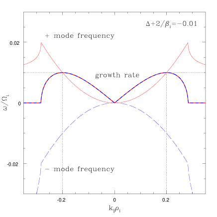
Figure 1: Frequencies (thin lines) and growth rates (bold lines) of the unstable firehose modes (red/solid: the “$+$” mode; blue/dashed: the “$-$” mode) given by equation (79). The instability parameter here is $\Delta+2/\beta_{i}=-0.01$. Dotted vertical lines indicate the wavenumber of fastest growth $k_{\rm p}=0.2$ (equation (81)) and the dotted horizontal lines the corresponding maximum growth rate $\gamma_{\rm max}={\rm Im}\,\omega_{\rm p}=0.01$ (equation (82)).

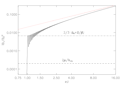
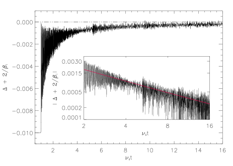
Figure 2: Left panel: evolution of the magnetic energy $\overline{|\mn@boldsymbol{B}_{1}^{\perp}|^{2}}/B_{0}^{2}=\sum_{k}|A_{k}|^{2}$ with time in a numerical solution of equations (86) and (87) with parameters (98); the time here is normalized using the collision frequency $\nu_{ii}$, not the cyclotron frequency $\Omega_{i}$; the two horizontal lines show the “collisional” (lower line) and “collisionless” (upper line) estimates for the energy at which the nonlinear feedback turns on: equations (89) and (90), respectively; the red dotted line shows the nonlinear asymptotic given by equation (91). Right panel: evolution of the instability parameter (pressure anisotropy) $\Delta+2/\beta_{i}$ in the same numerical solution. Inset: log-log plot of the evolution of $|\Delta+2/\beta_{i}|$; the red line shows the slope corresponding to $1/t$ (see equation (95)).

4.2 Linear theory

In the linear regime, we may neglect the second term in equation (73), so $\Delta=\Delta_{0}$. The linear dispersion relation for equation (77) is

$$\left[\omega^{2}-\frac{k_{\parallel}^{2}v_{\mathrm{th}i}^{2}}{2}\left(\Delta+\frac{2}{\beta_{i}}\right)\right]^{2}\!\!=\frac{k_{\parallel}^{4}v_{\mathrm{th}i}^{4}}{4}\frac{\omega^{2}}{\Omega_{i}^{2}}.$$ (78)

This has four roots out of which two are unstable when $\Delta+2/\beta_{i}<0$:

$$\frac{\omega}{\Omega_{i}}=\pm\frac{k^{2}}{4}+i\,\frac{|k|}{\sqrt{2}}\,\left|\Delta+\frac{2}{\beta_{i}}\right|^{1/2}\!\!\!\sqrt{1-\frac{k^{2}}{k_{0}^{2}}},$$ (79)

where $k=k_{\parallel}\rho_{i}$ and

$$k_{0}=2\sqrt{2}\left|\Delta+\frac{2}{\beta_{i}}\right|^{1/2}$$ (80)

(this linear dispersion relation was first obtained by Kennel & Sagdeev, 1967; Davidson & Völk, 1968). Unlike in the long-wavelength limit ($k_{\parallel}\rho_{i}\to 0$), there is now a real frequency (so the firehose perturbation propagates while its amplitude grows exponentially and the vector $\mn@boldsymbol{B}_{1}^{\perp}$ rotates; see section 4.3.1) and the growth rate has its peak at $k_{\rm p}=k_{0}/\sqrt{2}$, so

$$k_{\rm p} = 2\left|\Delta+\frac{2}{\beta_{i}}\right|^{1/2},$$ (81)

$$\omega_{\rm p} = \left(\pm 1+i\right)\left|\Delta+\frac{2}{\beta_{i}}\right|,$$ (82)

where the complex peak frequency $\omega_{\rm p}$ is in units of $\Omega_{i}$. At $k_{\parallel}\rho_{i}>k_{0}$, there is no growth and the firehose perturbations turn into purely propagating Alfvén waves (modified by pressure anisotropy and dispersive FLR corrections).

The dependence of the frequencies and growth rates of the two unstable modes on wavenumber given by equation (79) is plotted in figure 1 for a representative value of the instability parameter $\Delta+2/\beta_{i}=-0.01$ (this is the value used in the numerical solution of section 4.3.3).

It should be pointed out here that in this theory, there is no dissipation of the magnetic fluctuations excited by the firehose. The most unstable wavenumber is set by dispersive effects; the stable modes are undamped.

4.3 Nonlinear evolution and spectrum

4.3.1 Firehose turbulence equation in scalar form

Since the nonlinearity involves the spatially averaged perturbed magnetic energy, the firehose turbulence is compactly described in Fourier space not just in the linear but also in the nonlinear regime: this amounts to replacing $\nabla_{\parallel}^{2}\to-k_{\parallel}^{2}$ in equation (77) and $\overline{|\mn@boldsymbol{B}_{1}^{\perp}|^{2}}=\sum_{k_{\parallel}}|\mn@boldsymbol{B}_{1}^{\perp}(k_{\parallel})|^{2}$ in equation (73). A simple ansatz can now be used to convert equation (77) into scalar form. Let

$$\frac{B_{1x}}{B_{0}} = A_{k}(t)\cos\left(\frac{k^{2}}{4}\,t+\phi_{k}\right),$$ (83)

$$\frac{B_{1y}}{B_{0}} = A_{k}(t)\sin\left(\frac{k^{2}}{4}\,t+\phi_{k}\right),$$ (84)

where the axes $(x,y)$ in the plane perpendicular to $\mn@boldsymbol{\hat{b}}_{0}$ are chosen arbitrarily and we have non-dimensionalized wavenumbers and time:

$$k_{\parallel}\rho_{i}\to k,\quad\Omega_{i}t\to t.$$ (85)

This ansatz amounts to factoring out the rotation of the vector $\mn@boldsymbol{B}_{1}^{\perp}(k)$ (the first term in equation (79)). The wavenumber-dependent but time-independent phase $\phi_{k}$ is determined by the initial condition. We assume $\phi_{k}=\phi_{-k}$, so $A_{k}^{*}=A_{-k}$ must be satisfied to respect the fact that $\mn@boldsymbol{B}_{1}^{\perp}$ is a real field. The fluctuation amplitude $A_{k}(t)$ satisfies

$$\frac{\partial^{2}A_{k}}{\partial t^{2}} = \frac{k^{2}}{2}\left[-\left(\Delta+\frac{2}{\beta_{i}}\right)-\frac{k^{2}}{8}\right]A_{k},$$ (86)

$$\Delta(t) = \Delta_{0}+\frac{3}{2}\int_{0}^{t}\mathrm{d}t^{\prime}e^{-3\nu_{*}(t-t^{\prime})}\frac{\partial}{\partial t^{\prime}}\sum_{k}|A_{k}(t^{\prime})|^{2},$$ (87)

where $\nu_{*}=\nu_{ii}/\Omega_{i}=\rho_{i}/\lambda_{\mathrm{mfp}}$ and we remind the reader that $\Delta_{0}<0$. It is manifest in the form of equation (86) how the dispersion relation (79) (without the first term) is recovered. Note that there is no coupling between different wavenumbers modes in the sense that if a mode is not initially excited, it is never excited. The only effect that modes have on each other is via the sum over $k$ in equation (87), to which they all contribute.

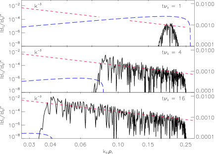
Figure 3: Left panel: spectrum of the magnetic fluctuation energy at three specific times ($t\nu_{ii}=1,4,16$) during the evolution shown in figure 2; red short-dashed lines show the $k^{-3}$ slope (equation (96)); blue long-dashed lines show the firehose growth rate (see equation (79)) for the instantaneous values of $\Delta+2/\beta_{i}$ at the times the spectra are plotted. Right panel: magnetic fluctuations in real space ($B_{1x}/B_{0}$ vs. $z$) at the same times as the spectra in the left panel.

4.3.2 Qualitative picture

Already on the basis of linear theory and the qualitative considerations of section 2.4, we can construct a fairly clear picture of the evolution of the firehose turbulence. Assuming a broad-band infinitesimal initial perturbation in $k$ space, at first, $\Delta=\Delta_{0}$ and all modes with $k<k_{0}$ (see equation (80)) will go unstable, with the fastest-growing one given by $k_{\rm p}=k_{0}/\sqrt{2}$. Eventually the amplitude in this mode reaches the level at which the back-reaction becomes important: approximating equation (87) by

$$\Delta(t)\simeq\Delta_{0}+\frac{1}{2\nu_{*}}\frac{\partial}{\partial t}\sum_{k}|A_{k}|^{2},$$ (88)

we find that the nonlinear contribution is comparable to $|\Delta_{0}+2/\beta_{i}|$ when (cf. equation (30)):

$$\sum_{k}|A_{k}|^{2}\simeq 2\left|\Delta_{0}+\frac{2}{\beta_{i}}\right|\frac{\nu_{*}}{\gamma_{\rm max}}=\frac{2\nu_{ii}}{\Omega_{i}}=\frac{2\rho_{i}}{\lambda_{\mathrm{mfp}}},$$ (89)

where $\gamma_{\rm max}$ is the imaginary part of $\omega_{\rm p}$ given by equation (82). Equation (89) only gives a good estimate of the critical amplitude if $3\nu_{*}$ is larger or not too much smaller than $\gamma_{\rm max}$ (collisions are sufficiently strong). If $\nu_{*}\ll\gamma_{\rm max}$ (as a subsidiary limit within our $\epsilon$ ordering), then a better approximation than equation (88) is to replace the collisional relaxation exponent in equation (87) by unity, which gives

$$\sum_{k}|A_{k}|^{2}\simeq\frac{2}{3}\left|\Delta_{0}+\frac{2}{\beta_{i}}\right|.$$ (90)

Once the nonlinear feedback becomes active, exponential growth must cease and secular growth starts because the anisotropy must be kept close to marginal: using equation (88), we find, to dominant order,

$$\Delta\simeq-\frac{2}{\beta_{i}}\quad\Rightarrow\quad\sum_{k}|A_{k}|^{2}\simeq 2\left|\Delta_{0}+\frac{2}{\beta_{i}}\right|\nu_{*}t.$$ (91)

This is valid regardless of which of the two estimates (89) or (90) of the amplitude at the onset of nonlinearity was appropriate. This is because the effective growth rate associated with the secular growth decreases with time and so we will always eventually end up in the regime where the collisional relaxation exponent in equation (87) is faster than the magnetic energy growth and equation (88) gives a good approximation of equation (87).

The evolution of the fluctuation spectrum must be consistent with equation (91). As the magnitude of the total pressure anisotropy $\Delta$ approaches the marginal value, both the cutoff wavenumber $k_{0}(t)$ and the most unstable wavenumber $k_{\rm p}(t)$ decrease, as they can still be estimated by equations (80) and (81) with $\Delta=\Delta(t)$. The modes whose growth has been thus switched off become oscillatory: from equation (86), it is obvious that for $k\gg k_{0}(t)$,

$$A_{k}=c_{1}e^{ik^{2}t/4}+c_{2}e^{-ik^{2}t/4},$$ (92)

where $c_{1}$ and $c_{2}$ are integration constants and $c_{1}^{*}=c_{2}$ because $A_{k}^{*}=A_{-k}$ (note that this oscillation of the amplitude is superimposed on the oscillation with the same frequency that was factored out in equations (83–84)). Since these modes oscillate in time at a rate that is much larger than the rate of change of the anisotropy, they no longer contribute to the feedback term in equation (87).

Thus, as the range of growing modes, peaked at $k_{\rm p}(t)$ and cut off at $k_{0}(t)$, sweeps from large to small wavenumbers, they leave behind a spectrum of effectively passive oscillations, whose amplitude no longer changes. Since there is no fixed special scale in the problem (except initial most unstable wavenumber), one expects the evolution to be self-similar and the spectrum a power law. It is not hard to determine its exponent. Let $|A_{k}|^{2}\sim k^{-\alpha}$. Since the total energy must grow linearly (equation (91))

$$\sum_{k}|A_{k}|^{2}\sim k_{\rm p}^{1-\alpha}\sim t\quad\Rightarrow\quad k_{\rm p}\sim t^{-1/(\alpha-1)}$$ (93)

(this is valid if $\alpha>1$; the extra power of $k$ comes from the integration over wavenumbers). On the other hand, for the fastest-growing mode, we must have, assuming secular growth,

$$\frac{1}{A_{k_{\rm p}}}\frac{\partial A_{k_{\rm p}}}{\partial t}\sim\frac{1}{t}\sim\gamma_{\rm max}\sim\left|\Delta+\frac{2}{\beta_{i}}\right|,$$ (94)

where the last relation follows from equation (82). This gives us a prediction for the time evolution of the residual pressure anisotropy and, via equation (81), of the most unstable wavenumber (the infrared cutoff of the spectrum):

$$\left|\Delta+\frac{2}{\beta_{i}}\right|\sim\frac{1}{t},\quad k_{\rm p}\sim\frac{1}{\sqrt{t}}.$$ (95)

The only way to reconcile equations (93) and (95) is to set $\alpha=3$. Thus, we expect the one-dimensional firehose turbulence spectrum to scale as

$$|A_{k}|^{2}\sim k^{-3}.$$ (96)

The secular growth of the firehose fluctuations will continue until our asymptotic expansion becomes invalid, i.e., when the fluctuation amplitude is no longer small. From equation (91), this happens at $t\sim\left(\nu_{ii}|\Delta_{0}+2/\beta_{i}|\right)^{-1}\sim|\gamma_{0}|^{-1}$, where dimensions have been restored. This is the time scale of the large-scale dynamics. Thus, as we have already explained in section 2.4, there is no saturation of the firehose fluctuations on any faster time scale. Unsurprisingly, at the same time as the fluctuation amplitude becomes large enough to break our ordering, the scale of the fluctuations also breaks the ordering: substituting the above time scale into equation (95), $k_{\parallel}\rho_{i}\sim(|\gamma_{0}|/\Omega_{i})^{1/2}\sim\epsilon^{2}$, or $k_{\parallel}\lambda_{\mathrm{mfp}}\sim 1$, while our original ordering assumption was $k_{\parallel}\rho_{i}\sim\epsilon$, or $k_{\parallel}\lambda_{\mathrm{mfp}}\sim 1/\epsilon$ (see equation (54)).

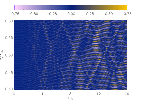
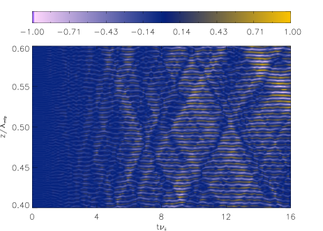
Figure 4: Left panel: contour plot of the time evolution of the firehose turbulence for the numerical solution discussed in section 4.3.3 — the vertical axis is space (the middle fifth of our entire periodic domain), horizontal axis is time, the colours respresent the value of $B_{1x}/B_{0}$. Right panel: the same plot for the gyrothermal turbulence discussed in section 5.3.3. Note that, as explained in the text, the firehose turbulence exhibits a gradual coarsening of the dominant structure with time, while the gyrothermal turbulence ends up dominated by a single scale.

4.3.3 Numerical solution

The firehose turbulence equation (86) is one-dimensional, so it is very easy to solve numerically; equation (87) is most conveniently solved in a differential form:

$$\frac{\partial}{\partial t}\biggl{(}\Delta-\frac{3}{2}\sum_{k}|A_{k}|^{2}\biggr{)}=-3\nu_{*}(\Delta-\Delta_{0})$$ (97)

with the initial condition $\Delta(0)=\Delta_{0}$. Here we describe the results obtained from such a numerical calculation with the following parameters:

$$\Delta_{0}=-0.02,\quad\frac{2}{\beta_{i}}=0.01,\quad\nu_{*}=\frac{\rho_{i}}{\lambda_{\mathrm{mfp}}}=0.0001.$$ (98)

This means that the maximum wavenumber at which firehose fluctuations can be excited is $k_{0}\simeq 0.28$ (equation (80); see figure 1). We solve equation (86) for 1024 wavenumbers in a periodic domain of size $\lambda_{\mathrm{mfp}}$, so the smallest and the largest wavenumbers are (still normalized to $\rho_{i}$) $k_{\rm min}=2\pi\rho_{i}/\lambda_{\mathrm{mfp}}\simeq 0.00063$ and $k_{\rm max}\simeq 0.32$. The initial conditions are random amplitudes in each wavenumber (satisfying the reality condition $A_{-k}=A_{k}^{*}$). Note that with the parameters (98), our ordering parameter is $\epsilon\sim 0.1$, so we have chosen a spatial scale separation between collisions and the Larmor motion that substantially exceeds $1/\epsilon^{2}$ formally mandated by our ordering (section 3.4). This does not break anything and is in fact more realistic for the physical parameters in weakly collisional plasmas of interest (section 2.1). It also widens the scale interval available to the firehose turbulence spectrum and ensures that even deep in the nonlinear regime, when the wavenumber of the firehose fluctuations drops substantially, there is still a healthy scale separation between them and the collisional dynamics.

The evolution of the total magnetic energy, $\overline{|\mn@boldsymbol{B}_{1}^{\perp}|^{2}}/B_{0}^{2}=\sum_{k}|A_{k}|^{2}$, is shown in figure 2 (left panel). Initially it grows exponentially at the (normalized) rate $\gamma_{\rm max}={\rm Im}\,\omega_{\rm p}$ (see equation (79); this part of the evolution is trivial and so not shown). The exponential growth is followed by a secular, linear in time, growth of the energy in accordance with equation (91). The energy at which this nonlinear regime starts is closer to the estimate given by equation (90) than by equation (89) because, as discussed above, we have taken a very small value of $\nu_{*}$. Note that in this and all subsequent figures, we have normalized time using the collision frequency $\nu_{ii}$, not the cyclotron frequency $\Omega_{i}$ — this is indicated explicitly in the figures and should cause no confusion to an attentive reader.

Figure 2 (right panel) shows the time evolution of the instability parameter $\Delta+2/\beta_{i}$. As expected, it is tending to the marginal stability value (zero). The inset shows that this approach to zero is consistent with the $1/t$ prediction (equation (95)).

The evolution of the spectrum of firehose fluctuations is illustrated by figure 3 (left panel). As anticipated in section 4.3.2, the spectral peak moves to smaller wavenumbers in the nonlinear regime. The spectrum extending from this moving peak to the original wavenumber of the fastest linear growth ($k_{\rm p}=0.2$; see equation (81)) is statistically stationary and consistent with the $k^{-3}$ power law predicted by equation (96). The instantaneous firehose growth rate is overplotted on the spectra in figure 3 (left panel) and confirms that the position of the spectral peak closely follows the wavenumber of the fastest instantaneous growth of the firehose instability.

Figure 3 (right panel) shows snapshots of one of the components ($B_{1x}$) of the perturbed magnetic field corresponding to the spectra in figure 3 (left panel). The emergence of increasingly larger-scale fluctuations is manifest. Perhaps a better illustration of this real-space evolution of the firehose turbulence is figure 4 (left panel), which is the space-time contour plot for the middle fifth of the domain.

4.4 Implications for momentum transport

Substituting the second-order pressure tensor calculated in section 3.7 into the large-scale momentum equation (71), we get

$$m_{i}n_{0i}\frac{\mathrm{d}\mn@boldsymbol{u}_{0i}}{\mathrm{d}t}=-\mn@boldsymbol{\nabla}\tilde{p}+\mn@boldsymbol{\nabla}\cdot\left[p_{0i}\mn@boldsymbol{\hat{b}}_{0}\mn@boldsymbol{\hat{b}}_{0}\left(\Delta+\frac{2}{\beta_{i}}\right)\right],$$ (99)

where, in the absence of density and temperature gradients, the total isotropic pressure $\tilde{p}=p_{2i}^{\perp}+B_{0}^{2}/8\pi$ is set by the condition $\mn@boldsymbol{\nabla}\cdot\mn@boldsymbol{u}_{0i}=0$, while the pressure anisotropy $\Delta$ is given by equation (73). A remarkable feature of equation (99) is that all of the effects of the magnetic field appear in the term proportional to $\Delta+2/\beta_{i}$, which is precisely the instability parameter that the small-scale firehose turbulence described in section 4.3 contrives to make vanish. In the marginal state that results, the tension force (the $2/\beta_{i}$ term) is almost entirely cancelled by the combined pressure anisotropy due to large- and small-scale fields. This suggests that in regions of the plasma where the firehose is triggered (i.e., where the magnetic field is locally decreased by the plasma motion), the plasma motions become effectively hydrodynamic, with magnetic-field lines unable to resist bending by the flows.

Since the cancellation of the second term in equation (99) by the firehose turbulence also effectively removes the (parallel) viscosity of the plasma, these hydrodynamic motions are not dissipated. In a turbulent situation, this should enable a cascade to ever smaller scales. Obviously, once this happens, the original motion that caused the negative pressure anisotropy to develop is supplanted by other, faster motions on smaller scales. The theory developed above eventually breaks down because the scale separation that formed the basis of our asymptotic expansion is compromised: while the fluid motions penetrate to smaller scales, the firehose fluctuations move to larger scales (see section 4.3).

Note also that the fluid motions produced by the turbulent cascade can give rise to both positive and negative pressure anisotropies — and so, to have a full description of their further evolution, we must know the effect on momentum transport not just of the firehose but also of the mirror and other instabilities triggered by positive pressure anisotropies (locally increasing magnetic field strength). This is still work in progress (the mirror case is considered by Rincon, Schekochihin & Cowley 2010). Another important adjustment to the viscous-stress reduction argument above has to do with the modification of the firehose instability by the parallel ion heat fluxes — we now proceed to investigate this.

5 Gyrothermal turbulence

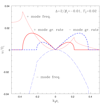
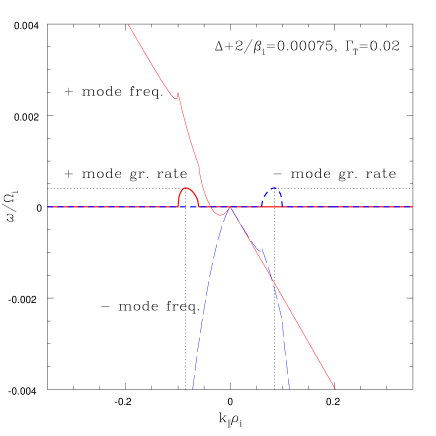
Figure 5: Left panel: frequencies (thin lines) and growth rates (bold lines) of the unstable firehose modes (red/solid: the “$+$” mode; blue/dashed: the “$-$” mode) given by equation (103); the parameters here are $\Delta+2/\beta_{i}=-0.01$ and $\Gamma_{T}=0.02$, so the instability parameter is $\Lambda=0.0054$ (equation (104)). Right panel: same, but for $\Delta+2/\beta_{i}=0.00075$, so $\Lambda=0.000025$ (close to marginal stability); dotted vertical lines indicate the wavenumber of fastest growth $k_{\rm p}=0.085$ (equation (109)) and the dotted horizontal lines the corresponding maximum growth rate $\gamma_{\rm max}={\rm Im}\,\omega_{\rm p}=0.0004$ (equation (110)).

5.1 Firehose turbulence equation with heat fluxes

As we briefly mentioned in section 3.7, allowing a non-zero ion temperature gradient along the unperturbed magnetic field leads to substantial modifications. These are of two kinds. First, as shown in Appendix A.2.13, the pressure anisotropy $\Delta_{0}$ caused by the large-scale dynamics contains contributions from the collisional parallel heat fluxes (proportional to $\mn@boldsymbol{\hat{b}}_{0}\cdot\mn@boldsymbol{\nabla}T_{0i}$) and from compressive motions (as we pointed out in footnote 9, the presence of a temperature gradient automatically implies a density gradient as well because of the requirement that pressure balance should be maintained; see equation (160) and Appendix A.2.12). Instead of equation (74), valid in the incompressible case, we must use the more general equation (187). This, however, does not change much: the unstable firehose fluctuations will grow in the manner described in section 4.3, first exponentially, then secularly, to compensate whatever pressure anisotropy is set up by the large-scale dynamics. The only change is the physical interpretation of the origin of the pressure anisotropy: as long as ion temperature gradients are present, the anisotropy is not tied exclusively to the change in the magnetic field. Physically, the heat-flux contributions to the anisotropy have to do with the fact that “parallel” and “perpendicular” heat flows along the magnetic-field lines somewhat differently and so imbalances between $p_{\perp}$ and $p_{\parallel}$ can occur — this can be seen already from the CGL equations (see Appendix A.2.15).

The second heat-flux-related modification of the theory developed thus far is more serious. It involves an additional contribution to the FLR term in the third-order pressure tensor (equation (75)) and, therefore, to the firehose turbulence equation (77). This contribution was derived in Appendix A.2.14, but suppressed in our previous discussion. It is given by equation (188) and consequently equation (77) now reads

$$\frac{\partial^{2}\mn@boldsymbol{B}_{1}^{\perp}}{\partial t^{2}} = \frac{v_{\mathrm{th}i}^{2}}{2}\,\nabla_{\parallel}^{2}\left[\left(\Delta+\frac{2}{\beta_{i}}\right)\mn@boldsymbol{B}_{1}^{\perp}\right.$$ (100)

$$+\left.\frac{1}{\Omega_{i}}\left(\frac{\partial\mn@boldsymbol{B}_{1}^{\perp}}{\partial t}-\Gamma_{T}\frac{v_{\mathrm{th}i}\nabla_{\parallel}\mn@boldsymbol{B}_{1}^{\perp}}{B_{0}}\right)\times\mn@boldsymbol{\hat{b}}_{0}\right].$$

We have introduced a dimensionless parameter measuring the magnitude of the parallel heat flux:

$$\Gamma_{T}=\frac{1}{2}\frac{v_{\mathrm{th}i}}{\nu_{ii}}\frac{\mn@boldsymbol{\hat{b}}_{0}\cdot\mn@boldsymbol{\nabla}T_{0i}}{T_{0i}}=\frac{1}{2}\frac{\lambda_{\mathrm{mfp}}}{l_{T}},$$ (101)

where $l_{T}$ is the parallel length scale of the ion temperature variation. We see that the functional form of the firehose turbulence equation is changed. We now proceed to study the effect of this change.

5.2 Linear theory: the gyrothermal instability

The linear dispersion relation for equation (100) is

$$\left[\omega^{2}-\frac{k_{\parallel}^{2}v_{\mathrm{th}i}^{2}}{2}\left(\Delta_{0}+\frac{2}{\beta_{i}}\right)\right]^{2}\!\!=\frac{k_{\parallel}^{4}v_{\mathrm{th}i}^{4}}{4}\frac{\left(\omega+k_{\parallel}v_{\mathrm{th}i}\Gamma_{T}\right)^{2}}{\Omega_{i}^{2}}.$$ (102)

Like in the case of equation (78), there are four roots of which two are potentially unstable:

$$\frac{\omega}{\Omega_{i}}=\pm\frac{k^{2}}{4}+i\,\frac{|k|}{\sqrt{2}}\sqrt{-\left(\Delta+\frac{2}{\beta_{i}}\right)\mp k\Gamma_{T}-\frac{k^{2}}{8}},$$ (103)

where $k=k_{\parallel}\rho_{i}$. Instability occurs at wavenumbers for which the expression under the square root is positive. There is an interval of such unstable wavenumbers if and only if

$$\Lambda\equiv\Gamma_{T}^{2}-\frac{1}{2}\left(\Delta+\frac{2}{\beta_{i}}\right)>0.$$ (104)

If this condition is satisfied, the “$+$” mode is unstable for

$$-4\left(\Gamma_{T}+\sqrt{\Lambda}\right)<k<-4\left(\Gamma_{T}-\sqrt{\Lambda}\right),$$ (105)

and the “$-$” mode for

$$4\left(\Gamma_{T}-\sqrt{\Lambda}\right)<k<4\left(\Gamma_{T}+\sqrt{\Lambda}\right).$$ (106)

where we have assumed, without loss of generality, that $\Gamma_{T}>0$. When $\Delta+2/\beta_{i}<0$, these two intervals intersect, so all modes with $|k|<k_{0}=4\left(\Gamma_{T}+\sqrt{\Lambda}\right)$ are unstable (others are pure propagating waves). When $\Delta+2/\beta_{i}>0$, the intervals are separated and there is an interval of stability at long wavelengths, viz., $|k|<4\left(\Gamma_{T}-\sqrt{\Lambda}\right)$.

What is remarkable about all this is that not only the stability conditions and specific expressions for the firehose growth rate are modified by heat flux, but the presence of the heat flux allows for instability even when firehose is stable, $\Delta+2/\beta_{i}>0$ (but positive pressure anisotropy not too large and $\beta_{i}$ not too small, subject to equation (104)). This instability, called the gyrothermal instability (GTI), leads to the growth of Alfvénically polarized fluctuations in the parameter regime in which they are otherwise stable (Schekochihin et al., 2010).

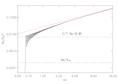
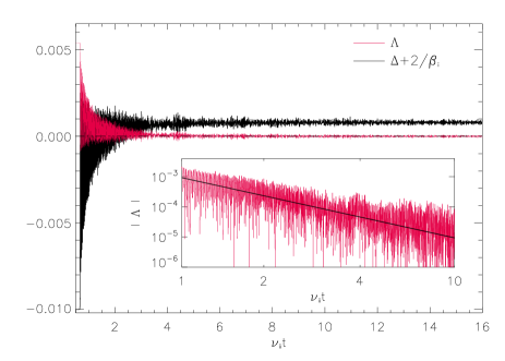
Figure 6: Left panel: evolution of the magnetic energy $\overline{|\mn@boldsymbol{B}_{1}^{\perp}|^{2}}/B_{0}^{2}=\sum_{k}|A_{k}|^{2}$ with time in a numerical solution of equations (112) and (113) with parameters (118); the red dotted line shows the nonlinear asymptotic given by equation (114); this figure is the GTI analog of figure 2 (left panel). Right panel: evolution of the instability parameter $\Lambda$ (pink) and the pressure anisotropy parameter $\Delta+2/\beta_{i}$ (black) in the same numerical solution. Inset: log-log plot of the evolution of $|\Lambda|$; the black line shows the slope corresponding to $1/t^{2}$ (see equation (116)).

The formulae for the wavenumber of the fastest-growing mode and the maximum growth rate for the combined firehose-GTI are straightforward to write down. As always with such formulae, they are not particularly illuminating in the general case, but are interesting in various asymptotic limits. When the firehose instability parameter $\Delta+2/\beta_{i}<0$ and its magnitude is much larger than $\Gamma_{T}^{2}$, the effect of the heat flux is a small correction to the firehose instability already described in section 4.2. Conversely, when $|\Delta+2/\beta_{i}|\ll\Gamma_{T}^{2}$, the GTI is dominant and, for the fastest growing mode,

$$k_{\rm p} \simeq \mp 6\Gamma_{T},$$ (107)

$$\omega_{\rm p} \simeq 9\Gamma_{T}^{2}\left(\pm 1+\frac{i}{\sqrt{3}}\right),$$ (108)

where $\omega_{\rm p}$ is normalized to $\Omega_{i}$. Finally, close to the marginal state, $\Lambda\to+0$, we have

$$k_{\rm p} \simeq \mp 4\Gamma_{T}\left(1+\frac{\Lambda}{\Gamma_{T}^{2}}\right),$$ (109)

$$\omega_{\rm p} \simeq 4\Gamma_{T}^{2}\left(\pm 1+\frac{i\sqrt{\Lambda}}{\Gamma_{T}}\right).$$ (110)

Note that, unlike the firehose, the GTI has a definite preferred wavenumber that does not change as marginal stability is approached.

Figure 5 (left panel) shows the dependence of the frequencies and growth rates of the two unstable modes on wavenumber for a set of parameters for which the instability is a hybrid of firehose and GTI (these are the parameters used in the numerical solution of section 5.3.3). Figure 5 (right panel) shows the same for the case in which the firehose is stable ($\Delta+2/\beta_{i}>0$) and that is very close to marginal stability: we see that the instability only exists in the immediate neighbourhood of the last unstable wavenumber given by equation (109).

5.3 Nonlinear evolution and spectrum

5.3.1 Firehose-GTI turbulence equation in scalar form

As happened in section 4.3.1, equation (100) can be reduced to one equation for a scalar field, although it is now a slightly more complicated transformation. Let us again non-dimensionalize time and space according to equation (85) and introduce new fields $A^{\pm}_{k}(t)$ as follows:

$$\frac{B_{1x}}{B_{0}}\pm i\,\frac{B_{1y}}{B_{0}}=A^{\pm}_{k}\exp\left[\mp i\left(\frac{k^{2}}{4}\,t+\phi_{k}\right)\right].$$ (111)

With the ansatz (111), equation (100) becomes

$$\frac{\partial^{2}A_{k}^{\pm}}{\partial t^{2}} = \frac{k^{2}}{2}\left[-\left(\Delta+\frac{2}{\beta_{i}}\right)\mp k\Gamma_{T}-\frac{k^{2}}{8}\right]A_{k}^{\pm},$$ (112)

$$\Delta(t) = \Delta_{0}+\frac{3}{2}\int_{0}^{t}\mathrm{d}t^{\prime}e^{-3\nu_{*}(t-t^{\prime})}\times$$ (113)

$$\qquad\qquad\times\,\,\frac{\partial}{\partial t^{\prime}}\sum_{k}\frac{|A_{k}^{+}(t^{\prime})|^{2}+|A_{k}^{-}(t^{\prime})|^{2}}{2}.$$

It is now manifest how the dispersion relation (103) emerges from equation (112). Unlike in the case of pure firehose turbulence ($\Gamma_{T}=0$), the evolution of the mode now depends on the sign of its real frequency — that is why we have two scalar equations. However, these equations have a symmetry: if we arrange initially that $A^{+}_{k}=A^{-}_{-k}$ (which we can always do by an appropriate choice of the phases $\phi_{k}$), then this relation will continue to be satisfied at later times. This also means that $A^{\pm}_{k}$ are real because, in order for $\mn@boldsymbol{B}_{1}^{\perp}$ to be a real field, we must have (from equation (111)) $(A^{+}_{k})^{*}=A^{-}_{-k}$ (we assume the phases satisfy $\phi_{k}=\phi_{-k}$). The conclusion is that it is enough to solve just one of the two equations (112) — either for the $+$ or the $-$ mode. The total energies of the two modes that enter equation (113) are equal.

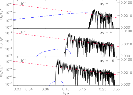
Figure 7: Left panel: spectrum of the magnetic fluctuation energy at three specific times ($t\nu_{ii}=1,4,16$) during the evolution shown in figure 6; red short-dashed lines show the $k^{-3}$ slope; blue long-dashed lines show the firehose/GTI growth rate (see section 5.2) for the instantaneous values of $\Delta+2/\beta_{i}$ at the times the spectra are plotted. Right panel: magnetic fluctuations in real space ($B_{1x}/B_{0}$ vs. $z$) at the same times as the spectra in the left panel. This figure is the GTI analog of figure 3.

5.3.2 Qualitative picture

The evolution of the firehose-GTI turbulence is easy to predict arguing along the same lines as we did in section 4.3.2. Let us consider the case when initially the pressure anisotropy is negative and $-(\Delta_{0}+2/\beta_{i})\gg 2\Gamma_{T}^{2}$, i.e., the instability parameter $\Lambda_{0}>0$ (given by equation (104) with $\Delta=\Delta_{0}$). In this regime, the heat flux does not matter and the evolution proceeds as in the case of the firehose turbulence: magnetic fluctuations grow and eventually the nonlinear feedback in equation (113) starts giving an appreciable positive contribution to the pressure anisotropy (estimates (89) and (90) for the fluctuation amplitude at which this happens are still valid). A $k^{-3}$ spectrum will then form, with the infrared cutoff (wavenumber of maximum growth) moving to larger scales and $|\Delta+2/\beta_{i}|$ decreasing (i.e., $\Delta+2/\beta_{i}$ increasing and thus becoming less negative).

The evolution of the gyrothermal fluctuations starts to differ from the pure firehose case after $|\Delta+2/\beta_{i}|$ becomes comparable to $\Gamma_{T}^{2}$. The GTI is now the dominant instability mechanism. Since the fluctuations continue growing, $\Delta+2/\beta_{i}$ continues to increase and will become positive, tending eventually to $2\Gamma_{T}^{2}$, so as to push the instability parameter $\Lambda$ (equation (104)) to zero and the GTI to its marginal state. As $\Lambda\to+0$, the growth is concentrated in a shrinking neighbourhood of the wavenumber $k_{\rm p}=4\Gamma_{T}$ (see equation (109)). This means that the spectrum stops spreading towards lower wavenumbers and its infrared cutoff stabilizes at $k_{\rm p}$. All the growth of magnetic energy is now provided by the growth of the one mode associated with $k_{\rm p}$, which will soon tower over the rest of the spectrum.

The growth is still secular: using equation (113) and the marginality condition $\Lambda=0$, we find to dominant order, analogously to equation (91),

$$\Delta\simeq 2\Gamma_{T}^{2}-\frac{2}{\beta_{i}}\quad\Rightarrow\quad\sum_{k}|A_{k}|^{2}\simeq 4\Lambda_{0}\nu_{*}t.$$ (114)

Finally, we can calculate the evolution of the residual $\Lambda$. Analogously to equation (94), the growing mode satisfies

$$\frac{1}{A_{k_{\rm p}}}\frac{\partial A_{k_{\rm p}}}{\partial t}\sim\frac{1}{t}\sim\gamma_{\rm max}\sim 4\Gamma_{T}\sqrt{\Lambda},$$ (115)

where we used equation (110) for $\gamma_{\rm max}$. Therefore,

$$\Lambda\sim\frac{1}{t^{2}}.$$ (116)

As in the case of the firehose turbulence, the secular growth will continue until the fluctuation amplitude is no longer small: $t\sim(\nu_{ii}\Lambda_{0})^{-1}\sim|\gamma_{0}|^{-1}$ (time scale of the large-scale dynamics). The key difference from the pure firehose case is that the fluctuations are now stuck at a microscopic spatial scale given by equation (109): restoring dimensions and using equation (101), the corresponding wavenumber is

$$k_{\parallel}\rho_{i}\sim\frac{\lambda_{\mathrm{mfp}}}{l_{T}}$$ (117)

(this scale is collisionless, $k_{\parallel}\lambda_{\mathrm{mfp}}\gg 1$, provided $l_{T}\ll\lambda_{\mathrm{mfp}}^{2}/\rho_{i}$; for galaxy clusters, this is always true as is easy to ascertain by using the numbers from section 2.1). Thus, the gyrothermal turbulence is essentially one-scale, in the sense that fluctuations at this one scale become energetically dominant as marginal stability is approached at late stages of the nonlinear evolution.

5.3.3 Numerical solution

We have solved equations (112) and (113) in a manner completely analogous to that described in section 4.3.3. The parameters we used are

$$\Delta_{0}=-0.02,\quad\frac{2}{\beta_{i}}=0.01,\quad\Gamma_{T}=0.02,$$

$$\nu_{*}=\frac{\rho_{i}}{\lambda_{\mathrm{mfp}}}=0.0001.$$ (118)

This implies that the instability parameter in the linear regime is $\Lambda=0.0054$ (equation (104)) and so the maximum unstable wavenumber is $k_{0}=4(\Gamma_{T}+\sqrt{\Lambda})\simeq 0.37$ (equations (105) and (106); see figure 5 (left panel)). Our numerical solution now has 2048 wavenumbers, so $k_{\rm min}\simeq 0.00063$ and $k_{\rm max}\simeq 0.64$.

As expected, the evolution of the total magnetic energy is similar to the case of pure firehose turbulence discussed in section 4.3.3: exponential, then secular growth (see equation (114)) — this is shown in figure 6 (left panel). The evolution of the instability parameter $\Lambda$ (equation (104)) towards its zero marginal value is given in figure 6 (right panel). The inset shows that this approach to zero is consistent with the $1/t^{2}$ prediction (equation (116)). Also shown in figure 6 (right panel) is the evolution of the pressure anisotropy parameter $\Delta+2/\beta_{i}$, which for the pure firehose used to be the instability parameter. Since $\Lambda\to 0$, it should tend to $2\Gamma_{T}^{2}=0.0008$ and it indeed does.

Finally, figure 7 (left panel) illustrates the evolution of the spectrum of firehose/gyrothermal fluctuations. It follows the scenario outlined in section 5.3.2. At first it is similar to the firehose turbulence spectrum with the spectral peak moving towards larger scales leaving behind a $k^{-3}$ spectrum. As the wavenumber of fastest growth $k_{\rm p}$ approaches the value corresponding to the near-marginal GTI, $k_{\rm p}=4\Gamma_{T}=0.08$ (see equation (109)), the peak stays there and continues growing, eventually dominating all other modes. The emergence of a one-scale sea of gyrothermal fluctuations is further illustrated by figure 4 (right panel), which shows what these fluctuations look like in real space as time progresses. The difference between them and the pure firehose fluctuations in figure 4 (left panel) is manifest: the gyrothermal ones stay at the same scale while the firehose ones become larger-scale as time progresses.

5.4 Implications for momentum and heat transport

Let us now revisit the discussion of the effect of plasma instabilities on the momentum transport modification attempted for the pure firehose in section 4.4. As before, the combined large-scale viscous and Maxwell stress is contained in the second term on the right-hand side of equation (99). However, with parallel ion heat fluxes present, the nonlinear evolution of the GTI pushes the quantity $\Delta+2/\beta_{i}$ not to zero but to a positive value $2\Gamma_{T}^{2}$, corresponding to the marginal state $\Lambda=0$ (equation (114)). Since any smaller value of $\Delta+2/\beta_{i}$ is GTI unstable, this leads to a curious conclusion that the momentum transport is now effectively determined by the ion heat flux:

$$m_{i}n_{0i}\frac{\mathrm{d}\mn@boldsymbol{u}_{0i}}{\mathrm{d}t} = -\mn@boldsymbol{\nabla}\tilde{p}+\mn@boldsymbol{\nabla}\cdot\left(p_{0i}\mn@boldsymbol{\hat{b}}_{0}\mn@boldsymbol{\hat{b}}_{0}2\Gamma_{T}^{2}\right)$$ (119)

$$= -\mn@boldsymbol{\nabla}\tilde{p}+\mn@boldsymbol{\nabla}\cdot\left[\mn@boldsymbol{\hat{b}}_{0}\mn@boldsymbol{\hat{b}}_{0}\frac{n_{0i}\left(\mn@boldsymbol{\hat{b}}_{0}\cdot\mn@boldsymbol{\nabla}T_{0i}\right)^{2}}{m_{i}\nu_{ii}^{2}}\right],$$

where we used equation (101) for $\Gamma_{T}$. This equation has to be supplemented with the transport and pressure-balance equations for $n_{0i}$, $T_{0i}$ and $\tilde{p}$ as explained in Appendix A.2.12.

Equation (119) probably merits a careful study (which is outside the scope of this paper), but we would like to accompany it with a very important caveat. Since pressure anisotropy in the nonlinear state of the GTI can be positive, other plasma instabilities may be triggered. Thus, if $\Delta>1/\beta_{i}$, i.e., if $\Gamma_{T}^{2}>3/(2\beta_{i})$, the plasma will be mirror unstable (see Hellinger, 2007, and references therein). The magnetic fluctuations that the mirror instability produces are different from the GTI both in polarization ($\delta B_{\parallel}$, not $\delta B_{\perp}$) and scale ($k_{\perp}\gg k_{\parallel}$, $k_{\perp}\rho_{i}\sim(\Delta-1/\beta_{i})^{1/2}$, $k_{\parallel}\rho_{i}\sim\Delta-1/\beta_{i}$ for the mirror, whereas for the GTI we had $k_{\perp}=0$, $k_{\parallel}\rho_{i}\simeq 4\Gamma_{T}$). How they saturate and what they do to the effective pressure anisotropy is a matter under active current investigation (Califano et al., 2008; Istomin, Pokhotelov & Balikhin, 2009; Rincon, Schekochihin & Cowley, 2010) — and it is completely unknown how mirror and gyrothermal fluctuations might coexist.

The key question is whether the pressure anisotropy will be set by the GTI or the mirror marginal condition and if it is set by the latter ($\Delta=1/\beta_{i}$, as, e.g., seems to be indicated by the solar wind data; see Hellinger et al. 2006; Bale et al. 2009), then whether a turbulent plasma has a way of suppressing the GTI by adjusting not the pressure anisotropy, but the heat flux to the marginal condition: $\Gamma_{T}^{2}=3/(2\beta_{i})$. This raises the possibility that not only the pressure anisotropy but also the (ion) heat fluxes are determined by the marginal stability conditions of the firehose/GTI and mirror. Thus, plasma instabilities may be the crucial factor in setting both the momentum and heat transport properties of a weakly collisional plasma. We stress, however, that under the assumptions adopted in this paper, we have not produced a nonlinear mechanism for changing the ion heat flux and this remains a subject for future work.

6 Discussion and comparison with previous work

6.1 Marginal stability via particle scattering or via changing field structure?

It is not in itself particularly surprising that the nonlinear effect of an instability driven by pressure anisotropy is to produce fluctuations that effectively pin this pressure anisotropy at a value corresponding to marginal stability. Besides having direct observational support in the solar wind (Gary et al., 2001; Kasper, Lazarus & Gary, 2002; Marsch, Ao & Tu, 2004; Hellinger et al., 2006; Matteini et al., 2007; Bale et al., 2009), it makes sense as a fundamental theoretical expectation (Le Châtelier’s principle). One may be tempted to proceed to another, seemingly as reasonable, theoretical expectation that the mechanism for achieving this marginal state must be pitch-angle scattering of particles by the fluctuations leading to isotropization of pressure. While indeed physically reasonable, this is, however, not an inevitable conclusion. As we have shown above, particle scattering is, in fact, not the way the $k_{\perp}=0$ firehose fluctuations make pressure anisotropy marginal (under the ordering assumptions we have adopted). Instead, the marginal state is achieved via a modification of the structure of the magnetic field: namely, secular growth of the microscale fluctuations cancels on average the decrease in the mean field that produced the pressure anisotropy thus pushing the latter to its marginal value. This was explained on an intuitive level in section 2.4 and the subsequent analytically rigorous developments showed that intuition to be correct.

Considering this result, we must recognize it as physically reasonable on the following grounds. A particle travelling in a magnetic field will traverse a fluctuation with a given $k_{\parallel}$ over time $\sim 1/k_{\parallel}v_{\mathrm{th}i}$. This time is much longer than the ion cyclotron period if $k_{\parallel}v_{\mathrm{th}i}\ll\Omega_{i}$, or, equivalanetly, if $k_{\parallel}\rho_{i}\ll 1$. If this condition is satisfied and if the frequency of the fluctuation $\omega\ll\Omega_{i}$, the fluctuation cannot change the first adiabatic invariant $\mu=v_{\perp}^{2}/2B$ of the particle, so there cannot be very much pitch-angle scattering. In our calculation, as the pressure anisotropy (or, more precisely, the instability parameters $\Delta+2/\beta_{i}$ and $\Gamma_{T}$) were small, the parallel scale of the fluctuations generated by the $k_{\perp}=0$ firehose or gyrothermal instabilities was substantially larger than the Larmor scale (see sections 4.2 and 5.2) and, in the case of the firehose, it increased further in the nonlinear regime (see section 4.3.2). Thus, $k_{\parallel}\rho_{i}\ll 1$ was satisfied at all times (as was $\omega\ll\Omega_{i}$), the plasma remained magnetized and pitch-angle scattering ineffective, so the rearrangement of the field structure was the only device available to the system to counteract the pressure anisotropy drive. It is possible that the oblique firehose (which is much harder to treat analytically than the parallel one) might produce fluctuations at the ion Larmor scale, so particle scattering by firehose fluctuations is not completely ruled out, but it certainly does not happen for the $k_{\perp}=0$ case to which we have limited the scope of the present investigation.

How important is it to know whether particle scattering is present? Recently, in the context of accretion-disc physics, Sharma et al. (2006, 2007) proposed an ad hoc closure for numerical simulations, constraining the pressure anisotropy to lie within the marginal stability boundaries via artificial dissipation in the pressure equations (the CGL equations given in Appendix A.2.15). They argued that this was justified if it could be shown microphysically that plasma instabilities (in their case, ion cyclotron and firehose) produced fluctuations at the ion Larmor scale, where pitch-angle scattering of particles off the fluctuation “foam” isotropized pressure. As we have explained, our results for the parallel ($k_{\perp}=0$) firehose do not support this picture. However, it is not obvious that the validity of a closure based on the average pressure anisotropy being maintained at the marginal level must be predicated on the presence of particle scattering. As we have shown above, a sea of secularly growing magnetic fluctuations far above the Larmor scale can produce the same effect. This, of course, does not excuse us from having to find the right microphysical theory for pressure isotropization if we are ever to have anything more than a plausible closure imposed by fiat.

One example of a context in which the presence or absence of scattering matters greatly is viscous heating of the plasma. The heating depends both on the pressure anisotropy and on the collision frequency (it is $\propto\nu_{ii}\Delta^{2}$; see Kunz et al. 2011), so, in order to calculate it correctly, we must know whether only the pressure anisotropy or also the (effective) collision frequency is modified by the firehose fluctuations. Assuming the Coulomb collision frequency unchanged, Kunz et al. 2011 recently proposed a thermally stable heating mechanism for galaxy clusters (see a further short discussion in section 7.3.1). If microphysically justified in the most general case (i.e., not only for the parallel firehose, but also the oblique one, the mirror instability, etc.), this represents significant progress. Thus, having a detailed microphysical theory does make a difference not only for the analytical strength of the subject but also for explaining astronomically observed realities.

6.2 Quasilinear theories

The theory developed above is basically quasilinear in that the fluctuation amplitude is assumed small and it is found that such small fluctuations can drive the instability to a marginal state. There have been a number of quasilinear treatments of the firehose instability (Shapiro & Shevchenko, 1964; Kennel & Sagdeev, 1967; Davidson & Völk, 1968; Gary & Feldman, 1978; Quest & Shapiro, 1996), so it is perhaps useful to explain why they do not obtain similar results.

The approach in such theories is to consider a collisionless plasma with some initial distribution that has a negative pressure anisotropy (let us call it $\Delta_{0}<0$) and work out how it relaxes. The result is that a fluctuation level builds up, with

$$\frac{|\mn@boldsymbol{B}_{1}^{\perp}|^{2}}{B_{0}^{2}}=\frac{2}{3}\left|\Delta_{0}+\frac{2}{\beta_{i}}\right|,$$ (120)

which is small when the instability parameter $\Delta_{0}+2/\beta_{i}$ is small. This saturated fluctuation level suffices to marginalize the instability. This result is easily recovered in our theory if we formally set $\nu_{ii}=0$ in equation (73). This gives

$$\Delta(t)=\Delta_{0}+\frac{3}{2}\frac{\overline{|\mn@boldsymbol{B}_{1}^{\perp}(t)|^{2}}}{B_{0}^{2}}$$ (121)

and assuming saturation in the marginal state $\Delta=-2/\beta_{i}$, we recover equation (120). The classic work where this was first done is Shapiro & Shevchenko (1964) (a more detailed comparison is provided in Appendix A.2.16). We stress that in their calculation the saturation of the pressure anisotropy at the marginal level is not due to particle scattering any more than it was in ours because the fluctuations still have $k_{\parallel}\rho_{i}\ll 1$, $\omega\ll\Omega_{i}$ and so conserve $\mu$ (see section 6.1). The internal energy stored in the pressure anisotropy is transferred into magnetic fluctuations until the pressure anisotropy is marginal. The magnetic fluctuations then persist because under the adopted appriximations there is no dissipation of the magnetic field.

The difference in our approach is to include weak collisions and consider the case when the pressure anisotropy is constantly driven by the large-scale dynamics (which is physically where it comes from; see section 2.2). The steady level of the anisotropy is then set by the competition between collisions and the drive (equation (74)) and to offset this anisotropy and keep the instability marginal, the fluctuation level has to keep growing secularly rather than stay constant (the earlier quasilinear theories can then be interpreted to describe correctly what happens before one collision time has elapsed).

6.3 Driven anisotropy in a collisionless plasma

It is interesting to inquire what would happen if the anisotropy were driven (rather than just initially imposed) but collisions not strong enough to balance the drive and impose a steady anisotropy. Formally speaking, our theory breaks down in this case because the equilibrium distribution cannot be proved Maxwellian. However, that is a technical issue and one could, in fact, reformulate our theory as a near-marginal expansion in the instability parameter $|\Delta+2/\beta_{i}|$. We expect that equation (184) (or, equivalently, equation (191)), with the collisional relaxation term removed, would still describe the evolution of the anisotropy:

$$\frac{\partial\Delta}{\partial t}=3\gamma_{0}+\frac{3}{2}\frac{\partial}{\partial t}\frac{\overline{|\mn@boldsymbol{B}_{1}^{\perp}(t)|^{2}}}{B_{0}^{2}},$$ (122)

where $\gamma_{0}$ (assumed negative) is the drive — it contains all the terms in equation (184) due the large-scale dynamics. Under these conditions, the driven part of anisotropy is constantly increasing and so again the fluctuations will have to grow secularly in order to keep it at the marginal level:

$$\frac{3}{2}\frac{\overline{|\mn@boldsymbol{B}_{1}^{\perp}(t)|^{2}}}{B_{0}^{2}}=\left|3\int_{0}^{t}\mathrm{d}t^{\prime}\gamma_{0}(t^{\prime})+\frac{2}{\beta_{i}}\right|.$$ (123)

This will, of course, break down once the fluctuation level is no longer small or collisions catch up.

6.4 Other nonlinear theories and simulations

There exist a number of numerical studies of the nonlinear evolution of the firehose instability (Berezin & Vshivkov, 1976; Quest & Shapiro, 1996; Gary et al., 1998; Hellinger & Matsumoto, 2001; Horton, Xu & Wong, 2004; Horton et al., 2004; Matteini et al., 2006). They mostly adopted the same relaxation-of-initial-anisotropy approach as the quasilinear theories discussed above and the results they report are broadly consistent in that the magnetic fluctuation energy saturates at a level scaling with the size of the initial anisotropy (see equation (120)). A notable exception is the recent work of Matteini et al. (2006) who consider the anisotropy driven by the expansion of the solar wind — the fluctuation levels they see are probably well described by equation (123).

The spectrum of the firehose fluctuations has not previously been addressed analytically, but, perhaps vaguely in agreement with the results of section 4.3, some of the numerical evidence does point to the growing predominance of smaller wavenumbers in the nonlinear regime — as the anisotropy approaches marginal level (Quest & Shapiro, 1996; Matteini et al., 2006).

Finally, to our knowledge, the effect of heat fluxes on the nonlinear behaviour of the firehose instability, studied in section 5, has not been specifically considered before. Note that although the heat fluxes are present in the numerical simulations of Sharma et al. (2006, 2007), their momentum equation does not have the gyroviscous and gyrothermal terms that regularize the firehose at small scales and give rise to the gyrothermal instability. The appropriate modification to the fluid equations suggested by Schekochihin et al. (2010) should in principle enable one to study the spectrum of the firehose and GTI fluctuations numerically.

7 Astrophysical implications

7.1 Solar wind

Much of the observational evidence about the firehose instability comes from the measurements of pressure anisotropies and fluctuation levels in the solar wind. Since the wind is expanding, both the local density and the local magnetic-field strength are dropping, so one expects a negative pressure anisotropy to develop: this can be described by equation (122), where the drive is roughly $\gamma_{0}\sim-V_{\rm sw}/R$ (solar wind speed divided by the distance from the Sun) and the collisional relaxation is neglected. The evidence for this trend, negative pressure anisotropy developing with increasing distance from the Sun, is given by Matteini et al. (2007); a number of other papers also document the fact that the measured pressure anisotropies are bounded from below by the firehose marginal stability condition (Kasper, Lazarus & Gary, 2002; Hellinger et al., 2006; Bale et al., 2009).

Bale et al. (2009) found increased levels of ion-Larmor-scale magnetic fluctuations close to this stability boundary — presumably due to the firehose instability. There are also indications of an injection of energy into parallel wavenumbers just above the ion Larmor scale (Podesta, 2009; Wicks et al., 2010) — again, conceivably by the firehose instability. It is unclear how these firehose fluctuations coexist with the solar wind inertial- and dissipation-range turbulence — as our theoretical understanding of this turbulence is still largely based on assuming isotropic equilibrium distributions (see Schekochihin et al., 2009, and references therein). This is one of the contexts in which the absence of a complete microphysical theory of the firehose turbulence and its effect on the plasma motions is particularly acutely felt.

7.2 Accretion discs

Another such astrophysical context is hot accretion flows, in which the theoretical modelling of the long-standing problem of the angular momentum transport and radiative efficiency or inefficiency of the accretion has taken a new turn with the introduction of pressure anisotropies (Quataert, Dorland & Hammett, 2002; Sharma, Hammett & Quataert, 2003; Balbus, 2004; Islam & Balbus, 2005; Sharma et al., 2006, 2007). The numerical model of Sharma et al. (2006, 2007) consisted of a closure that pinned down the pressure anisotropies at marginal stability via artificial dissipation terms. As we explained in section 6.1, their assumption of microscale fluctuations scattering particles is not bourne out by the theory developed above for the parallel ($k_{\perp}=0$) firehose fluctuations, although it is not excluded for other instabilities and, in any event, a closure based on marginal stability is probably a sensible choice.

A key remaining unknown here is the fate of the microscale fluctuations over long (transport) time scales and the eventual structure of the tangled magnetic field that results — a crucial question for accretion theories because they require knowledge of the Maxwell and Braginskii stresses in order to estimate the rate of the angular momentum transport (Shakura & Sunyaev, 1973). The same problem of the magnetic-field structure arises in considerations of the ICM dynamics and magnetogenesis (see sections 2.1 and 7.3).

7.3 Galaxy clusters

In section 2, we discussed at length the basic properties of the galaxy cluster plasmas, the inevitability of pressure anisotropies and, therefore, plasma instabilities arising in a turbulent ICM, as well as the fundamental theoretical questions that this poses. These will not find their final resolution in this paper because it has only analyzed one of several plasma instabilities that must be understood. However, just like in the case of the solar wind and the accretion flows, an impatient astrophysicist can conceivably glimpse the contours of the eventual theory by constraining pressure anisotropies and possibly also heat fluxes by the marginal stability conditions of the plasma instabilities — with all the caveats and uncertainties already discussed above.

Let us discuss how far this approach can take us in answering the three classes of physical problems that were described at the beginning of section 2.1.

7.3.1 Regulation of cooling flows

The apparent refusal of the galaxy cluster cores to exhibit a cooling catastrophe (e.g., Peterson & Fabian, 2006) has long evaded a satisfactory theoretical explanation. A comprehensive review of the relevant literature is outside the scope of this brief discussion. It is probably fair to summarize the two main physical mechanisms invoked to explain the relatively weak drop in the ICM temperature between the bulk and the core as thermal conduction and some form of viscous conversion into heat of the mechanical energy injected into the ICM by the central active galactic nuclei (probably in a self-regulating way; see, e.g., Binney 2003; Kaiser & Binney 2003; Omma & Binney 2004; Ogrean et al. 2010; Teyssier et al. 2010 and the references in section 2.1). It is clear that the latter mechanism cannot be ignored because the thermal conductivity of the ICM is unlikely to be sufficiently large (e.g., Voigt & Fabian, 2004) and at any rate, thermal conduction is a thermally unstable mechanism of balancing radiative cooling. Kunz et al. (2011) recently proposed that if a sufficient amount of turbulent power is assumed to be available, the viscous heating, regulated by the pressure anisotropy and, therefore, by the marginal stability of the mirror and/or firehose instabilities, can balance the cooling in a thermally stable way. They also found that assuming such a balance leads to reasonable predictions of the magnetic field strength, magnitude of the turbulent velocities and the outer scale of the turbulence in the ICM.

7.3.2 Temperature fluctuations and the GTI

While detailed simulations of the turbulent ICM, bubble dynamics etc. similar to those of Sharma et al. (2006, 2007) for accretion flows have not been attempted, the marginal stability condition for the GTI (equation (104)) could perhaps be used to impose a lower bound on the typical scale of temperature fluctuations in the ICM (Schekochihin et al., 2010). Indeed, if the magnitude of the ion heat flux is limited so as to prevent the GTI from being unstable (see section 5.4), then from equations (104) and (101), we get

$$l_{T}\gtrsim\beta_{i}^{1/2}\lambda_{\mathrm{mfp}}\sim 5\times 10^{-4}\frac{T_{i}^{5/2}}{n_{i}^{1/2}B}\sim 1.4\times 10^{21}~{}{\rm cm},$$ (124)

where $n_{i}$ is in cm^-3, $T_{i}$ is in K, $B$ is in G, and the numerical value has been computed for the plasma parameters in the core of Hydra A discussed in section 2.1 (see equations (6) and (8)). Interestingly, kpc-scale temperature fluctuations are indeed observed in cool-core clusters (Simionescu et al., 2001; Fabian et al., 2006; Sanders et al., 2010a; Laganá, Andrade-Santos & Lima Neto, 2010). Furthermore, if we use in equation (124) the physical parameters appropriate for the bulk of the cluster plasma, rather than the cores (say, $T_{i}\sim 10^{8}$ K and $n_{i}\sim 10^{-3}$ cm^-3) we would get much larger scales — in the 100 kpc range, which is also consistent with reported observational values for the cluster bulk (Markevitch et al., 2003).

7.3.3 Magnetogenesis

In the presence of turbulence, the small-scale (fluctuation) dynamo mechanism generates a magnetic field — this is certainly true in an MHD fluid (e.g., Subramanian, Shukurov & Haugen, 2006; Brandenburg & Nordlund, 2009). How this mechanism works in a plasma susceptible to the microscale plasma instabilities remains a completely open problem. A rather speculative attempt by Schekochihin & Cowley (2006) to leapfrog the detailed microphysical derivations and model the large-scale dynamics based on the idea that the instabilities would always isotropize pressure towards marginal stability values led to a rather dramatic conclusion that the ICM might support self-accelerating, explosive dynamos. While this conclusion remains to be tested by more rigorous analytical approaches, it does illustrate the general conjecture that plasma instabilities are likely to result in radical changes of, rather than merely small corrections to, the large-scale dynamics of cosmic plasmas. A particular mystery in understanding the origin and structure of the magnetic field in the ICM is what determines the typical spatial scale of magnetic fluctuations, which observations suggest may be substantially smaller than the scale of the turbulent motions (see further discussion and references in Schekochihin & Cowley, 2006).

8 Conclusion

Let us recapitulate what this paper has achieved and how it relates to what was known previously. It has been appreciated for some time that macroscale turbulence of magnetized weakly collisional plasma (exemplified by the ICM) will naturally produce pressure anisotropies, which will in turn trigger firehose and mirror instabilities at spatial and temporal microscales (Hall & Sciama, 1979; Schekochihin et al., 2005, see extended discussion in sections 1 and 2). Since the pressure anisotropies are essentially due to local temporal change of the magnetic field strength, it is qualitatively intuitive that the nonlinear evolution of the instabilities is governed by the tendency to cancel this change on average; hence it follows that in a driven system (see discussion in section 6) the fluctuations must continue growing in the nonlinear regime, albeit secularly rather than exponentially (Schekochihin et al., 2008, see section 2.4).

In this paper, we have constructed a full ab initio (weakly) nonlinear kinetic theory of this process for the parallel ($k_{\perp}=0$) firehose instability, which is the simplest analytically tractable case. The evolution not only of the fluctuation energy, but also of the full spectrum of the resulting firehose turbulence has been worked out, including the effect of gradual spreading of the fluctuations to ever larger scales as the nonlinearly compensated pressure anisotropy approaches its marginal-stability value (section 4.3). We have also extended our kinetic calculation to include the effect of ion temperature gradients parallel to the magnetic field (parallel heat fluxes). As was pointed out recently, they lead to a new instability, the GTI, of parallel Alfvénic fluctutions (Schekochihin et al., 2010, see also section 5.2). Here we have constructed a nonlinear theory of its evolution, featuring again a secular growth of magnetic fluctuations, but this time developing a spectrum heavily dominated by a particular scale (section 5.3).

While a speculative discussion of the implications of these results for transport in a general magnetized plasma (sections 4.4–5.4) and for particular astrophysical systems (section 7) is possible, a full transport theory has to await, at the very least, the completion of similar ab initio kinetic investigations of the nonlinear evolution of the mirror instability (Rincon, Schekochihin & Cowley, 2010) and of the oblique ($k_{\perp}\neq 0$) firehose. Only then can one attempt to devise an effective mean field theory for the macroscale dynamics of cosmic plasmas based on solid microphysical foundations. A goal of this paper has been to establish a template for building these microphysical foundations.

In the meanwhile, it appears sensible to rely on (or at least consider reasonable) the semiquantitative closure approach to the macroscale dynamics based on the assumption that average pressure anisotropies and, probably, also heat fluxes, are set by the marginal stability conditions of the microscale plasma instabilities — an approach that has found strong observational support in the solar wind measurements (Gary et al., 2001; Kasper, Lazarus & Gary, 2002; Marsch, Ao & Tu, 2004; Hellinger et al., 2006; Matteini et al., 2007; Bale et al., 2009) and has already yielded nontrivial and possibly sensible physical predictions for the evolution of cosmic magnetism (Schekochihin & Cowley, 2006), accretion disk dynamics (Sharma et al., 2006, 2007), and the turbulence and heating in the intracluster medium (Lyutikov, 2007; Kunz et al., 2011) (see further discussion in section 7).

Appendix A Kinetic theory: detailed derivation

A.1 Electrons

A.1.1 Mass-ratio ordering

The kinetic equation (32) for electrons is (recall that $\mn@boldsymbol{v}$ is the peculiar velocity)

$$\begin{array}[]{cccccccccccccccccccc}\displaystyle{\frac{\partial f_{e}}{\partial t}}&+&\displaystyle{\mn@boldsymbol{u}_{e}\cdot\mn@boldsymbol{\nabla}f_{e}}&+&\displaystyle{\mn@boldsymbol{v}\cdot\mn@boldsymbol{\nabla}f_{e}}&-&\displaystyle{\Bigg{[}\frac{e}{m_{e}}}&\displaystyle{\bigg{(}\mn@boldsymbol{E}+\frac{\mn@boldsymbol{u}_{e}\times\mn@boldsymbol{B}}{c}}&+&\displaystyle{\frac{\mn@boldsymbol{v}\times\mn@boldsymbol{B}}{c}\bigg{)}}&+&\displaystyle{\frac{\partial\mn@boldsymbol{u}_{e}}{\partial t}}&+&\displaystyle{\mn@boldsymbol{u}_{e}\cdot\mn@boldsymbol{\nabla}\mn@boldsymbol{u}_{e}}&+&\displaystyle{\mn@boldsymbol{v}\cdot\mn@boldsymbol{\nabla}\mn@boldsymbol{u}_{e}\Bigg{]}\cdot}&\displaystyle{\frac{\partial f_{e}}{\partial\mn@boldsymbol{v}}}&=&\displaystyle{C[f_{e}],}\\ 1&&1&&\left(\frac{m_{e}}{m_{i}}\right)^{-\frac{1}{2}}&&&\left(\frac{m_{e}}{m_{i}}\right)^{-\frac{1}{2}}&&\left(\frac{m_{e}}{m_{i}}\right)^{-1}&&\left(\frac{m_{e}}{m_{i}}\right)^{\frac{1}{2}}&&\left(\frac{m_{e}}{m_{i}}\right)^{\frac{1}{2}}&&1&&&\left(\frac{m_{e}}{m_{i}}\right)^{-\frac{1}{2}}\end{array}$$ (125)

where we have labeled all terms according to their ordering in powers of $(m_{e}/m_{i})^{1/2}$, while taking $T_{e}\sim T_{i}$ The ordering has been done relative to $kv_{\mathrm{th}i}f_{e}$ and we have assumed

$$\frac{\partial}{\partial t}\sim\omega\sim kv_{\mathrm{th}i},\quad\mn@boldsymbol{\nabla}\sim k\sim\rho_{i}^{-1}\sim\left(\frac{m_{e}}{m_{i}}\right)^{1/2}\frac{eB}{m_{e}c\,v_{\mathrm{th}e}},\quad\mn@boldsymbol{u}_{e}\sim v_{\mathrm{th}i},\quad\mn@boldsymbol{v}\sim v_{\mathrm{th}e}\sim\left(\frac{m_{e}}{m_{i}}\right)^{-1/2}v_{\mathrm{th}i},\quad\mn@boldsymbol{E}\sim\frac{\mn@boldsymbol{u}_{e}\times\mn@boldsymbol{B}}{c},$$ (126)

$$\nu_{ei}\sim\nu_{ee}\sim\left(\frac{m_{e}}{m_{i}}\right)^{-1/2}\nu_{ii},\quad\nu_{ii}\sim\omega,$$ (127)

where $\nu_{ei}$ and $\nu_{ee}$ are the electron-ion and electron-electron collision frequencies (they determine the ordering of the collision integral on the right-hand side of equation (125)). We stress that these are formal orderings with respect to the mass-ratio expansion, not statements about the exact size of various quantities and their derivatives: thus, some of the quantities ordered as unity within the mass-ratio expansion (e.g., $k\rho_{i}$ or $\mn@boldsymbol{u}_{e}/v_{\mathrm{th}i}$) will be ordered small in the subsidiary $\epsilon$ expansion to be used in solving the ion kinetics (see section 3.4).

We now expand the electron distribution function in powers of $(m_{e}/m_{i})^{1/2}$: $f_{e}=f_{e}^{(0)}+f_{e}^{(1)}+\cdots$. It turns out that we can learn all we need to know from just the two lowest orders in the expansion of equation (125). Note that we do not expand any of the fields — exact $\mn@boldsymbol{E}$ and $\mn@boldsymbol{B}$ are kept.

A.1.2 Order $(m_{e}/m_{i})^{-1}$: gyrotropic electrons

To this order, equation (125) is

$$-\frac{e}{m_{e}}\frac{\mn@boldsymbol{v}\times\mn@boldsymbol{B}}{c}\cdot\frac{\partial f_{e}^{(0)}}{\partial\mn@boldsymbol{v}}=-\Omega_{e}\,\frac{\partial f_{e}^{(0)}}{\partial\vartheta}=0,$$ (128)

where $\Omega_{e}=-eB/m_{e}c$ and $\vartheta$ is the gyroangle variable. Thus, in this order, we have learned that the lowest-order electron distribution function is gyrotropic (does not depend on $\vartheta$).

A.1.3 Order $(m_{e}/m_{i})^{-1/2}$: Maxwellian electrons

To this order, equation (125) is

$$\mn@boldsymbol{v}\cdot\mn@boldsymbol{\nabla}f_{e}^{(0)}-\frac{e}{m_{e}}\left(\mn@boldsymbol{E}+\frac{\mn@boldsymbol{u}_{e}\times\mn@boldsymbol{B}}{c}\right)\cdot\frac{\partial f_{e}^{(0)}}{\partial\mn@boldsymbol{v}}-\Omega_{e}\frac{\partial f_{e}^{(1)}}{\partial\vartheta}=C[f_{e}^{(0)}].$$ (129)

Let us multiply this equation by $1+\ln f_{e}^{(0)}$ and integrate over the entire phase space. This gives

$$\int\int\mathrm{d}^{3}\mn@boldsymbol{r}\mathrm{d}^{3}\mn@boldsymbol{v}C[f_{e}^{(0)}]\ln f_{e}^{(0)}=0$$ (130)

because the left-hand side of equation (129) is an exact divergence in the phase space. Let us recall that, according to Boltzmann (1872) $H$-theorem,

$$\frac{\mathrm{d}}{\mathrm{d}t}\int\int\mathrm{d}^{3}\mn@boldsymbol{r}\mathrm{d}^{3}\mn@boldsymbol{v}f_{e}\ln f_{e}=\int\int\mathrm{d}^{3}\mn@boldsymbol{r}\mathrm{d}^{3}\mn@boldsymbol{v}C[f_{e}]\ln f_{e}\leq 0,$$ (131)

where the inequality becomes equality only for a local Maxwellian distribution (the proof for plasmas can be found in, e.g., Longmire 1963). Therefore, equation (130) implies that $f_{e}^{(0)}$ is a local Maxwellian:

$$f_{e}^{(0)}=\frac{n_{e}}{\left(\pi v_{\mathrm{th}e}^{2}\right)^{3/2}}\,e^{-v^{2}/v_{\mathrm{th}e}^{2}},\quad v_{\mathrm{th}e}=\sqrt{\frac{2T_{e}}{m_{e}}}.$$ (132)

Since $v$ is peculiar velocity, the mean flow $\mn@boldsymbol{u}_{e}$ has already been accounted for. Note that the perturbation expansion of $f_{e}$ can always be constructed in such a way that $n_{e}$ and $T_{e}$ in equation (132) are the exact density and temperature of the electron distribution.

A.1.4 Isothermal electrons

More can be learned about the electrons without going to higher orders. Let us now substitute the expression (132) for $f_{e}^{(0)}$ into equation (129) and gyroaverage this equation, $(1/2\pi)\int\mathrm{d}\vartheta$, to eliminate the term containing $f_{e}^{(1)}$:

$$v_{\parallel}\mn@boldsymbol{\hat{b}}\cdot\mn@boldsymbol{\nabla}f_{e}^{(0)}+\frac{e}{m_{e}}\mn@boldsymbol{E}\cdot\mn@boldsymbol{\hat{b}}\,\frac{2v_{\parallel}}{v_{\mathrm{th}e}^{2}}\,f_{e}^{(0)}=\left[\frac{\mn@boldsymbol{\hat{b}}\cdot\mn@boldsymbol{\nabla}n_{e}}{n_{e}}+\left(\frac{v^{2}}{v_{\mathrm{th}e}^{2}}-\frac{3}{2}\right)\frac{\mn@boldsymbol{\hat{b}}\cdot\mn@boldsymbol{\nabla}T_{e}}{T_{e}}+\frac{eE_{\parallel}}{T_{e}}\right]v_{\parallel}f_{e}^{(0)}=0,$$ (133)

where $E_{\parallel}=\mn@boldsymbol{E}\cdot\mn@boldsymbol{\hat{b}}$. Since equation (133) must hold for all $v$, it follows from it that

$$E_{\parallel}=-\frac{T_{e}\mn@boldsymbol{\hat{b}}\cdot\mn@boldsymbol{\nabla}n_{e}}{en_{e}},$$ (134)

$$\mn@boldsymbol{\hat{b}}\cdot\mn@boldsymbol{\nabla}T_{e}=0.$$ (135)

The second equation means that electrons (to lowest order) are isothermal along the magnetic-field lines, a standard outcome of the mass-ratio expansion (Snyder & Hammett, 2001; Schekochihin et al., 2009), valid up to parallel scales $\sim\lambda_{\mathrm{mfp}}(m_{i}/m_{e})^{1/2}$ (the electron thermal conduction scale; see, e.g., Lithwick & Goldreich 2001; Schekochihin et al. 2009). For our fiducial ICM parameters, we have $\lambda_{\mathrm{mfp}}(m_{i}/m_{e})^{1/2}\sim 6\times 10^{21}$ cm, which is larger than the scale $l$ of the motions that have the highest rate of strain (see section 2.1). For turbulent plasmas, this implies globally isothermal electrons ($T_{e}={\rm const}$) because the field lines are stochastic. We will adopt this assumption of globally isothermal electrons in all our calculations.

A.1.5 Generalized Ohm’s law

Let us again go back to equation (129), multiply it by $m_{e}\mn@boldsymbol{v}$ and integrate over the velocity space. The result is the electron momentum equation to lowest order in the mass-ratio expansion:

$$en_{e}\left(\mn@boldsymbol{E}+\frac{\mn@boldsymbol{u}_{e}\times\mn@boldsymbol{B}}{c}\right)=-\mn@boldsymbol{\nabla}\cdot\int\mathrm{d}^{3}\mn@boldsymbol{v}m_{e}\mn@boldsymbol{v}\mn@boldsymbol{v}f_{e}^{(0)}=-\mn@boldsymbol{\nabla}p_{e}=-T_{e}\mn@boldsymbol{\nabla}n_{e},$$ (136)

where the electron pressure is isotropic because the distribution is Maxwellian, $p_{e}=n_{e}T_{e}$, and the gradient only affects $n_{e}$ because $T_{e}=const$ (section A.1.4). Note that equation (134) is simply the parallel part of equation (136). Equation (136) is the generalized Ohm’s law, equation (37). We have thus arrived at the starting point of the derivation in section 3.2.

A.2 Ions

A.2.1 Ordering

The kinetic equation (32) for ions is

$$\begin{array}[]{lcccccccccccccccccccc}&\displaystyle{\frac{\partial f_{i}}{\partial t}}&+&\displaystyle{\mn@boldsymbol{u}_{i}\cdot\mn@boldsymbol{\nabla}f_{i}}&+&\displaystyle{\mn@boldsymbol{v}\cdot\mn@boldsymbol{\nabla}f_{i}}&+&\displaystyle{\Bigg{[}\frac{Ze}{m_{i}}}&\displaystyle{\bigg{(}\mn@boldsymbol{E}+\frac{\mn@boldsymbol{u}_{i}\times\mn@boldsymbol{B}}{c}}&+&\displaystyle{\frac{\mn@boldsymbol{v}\times\mn@boldsymbol{B}}{c}\bigg{)}}&-&\displaystyle{\frac{\partial\mn@boldsymbol{u}_{i}}{\partial t}}&-&\displaystyle{\mn@boldsymbol{u}_{i}\cdot\mn@boldsymbol{\nabla}\mn@boldsymbol{u}_{i}}&-&\displaystyle{\mn@boldsymbol{v}\cdot\mn@boldsymbol{\nabla}\mn@boldsymbol{u}_{i}\Bigg{]}\cdot}&\displaystyle{\frac{\partial f_{i}}{\partial\mn@boldsymbol{v}}}&=&\displaystyle{C[f_{i}],}\\ \\ \mathrm{Equil.}&\epsilon^{3}&&\epsilon^{3}&&\epsilon^{2}&&&\epsilon^{2}&&\epsilon^{-1}&&\epsilon^{4}&&\epsilon^{4}&&\epsilon^{3}&&&\epsilon\\ \mathrm{Pert.}&\epsilon^{2}&&\epsilon^{2}&&\epsilon&&&\epsilon&&1&&\epsilon^{3}&&\epsilon^{3}&&\epsilon^{2}&&&\epsilon^{2}\\ \end{array}$$ (137)

where we have labeled all terms according to their ordering in powers of $\epsilon$. The ordering has been done relative to $k_{\parallel}v_{\mathrm{th}i}f_{i}$ using the assumptions explained in section 3.4. The first row of orderings in equation (137) applies to the equilibrium (lowest-order) quantities and their gradients. The second row gives the lowest order in which perturbed quantities appear in each term of the kinetic equation.

A.2.2 Expansion of the Lorentz force

A particular explanation is in order regarding the ordering and the expansion of the Lorentz force. The Lorentz force is given in terms of $n_{i}$ and $\mn@boldsymbol{B}$ by equation (40). Expanding this equation in $\epsilon$, we have to three lowest orders

$$\begin{array}[]{cccccccccccc}\displaystyle{\frac{Ze}{m_{i}}\left(\mn@boldsymbol{E}+\frac{\mn@boldsymbol{u}_{i}\times\mn@boldsymbol{B}}{c}\right)}&=&-&\displaystyle{\frac{ZT_{e}\mn@boldsymbol{\nabla}n_{1i}}{m_{i}\left(n_{0i}+n_{1i}+n_{2i}\right)}}&-&\displaystyle{\frac{ZT_{e}\mn@boldsymbol{\nabla}\left(n_{0i}+n_{2i}\right)}{m_{i}\left(n_{0i}+n_{1i}\right)}}&-&\displaystyle{\frac{ZT_{e}\mn@boldsymbol{\nabla}n_{3i}}{m_{i}n_{0i}}}&+&\displaystyle{v_{A}^{2}\nabla_{\parallel}\frac{\mn@boldsymbol{B}_{1}^{\perp}}{B_{0}}}&+&\cdots,\\ \\ &&&\epsilon&&\epsilon^{2}&&\epsilon^{3}&&\epsilon^{3}&&\end{array}$$ (138)

where we have used $B_{1}^{\parallel}=0$ (see equation (59)). The ordering of the Lorentz force in equation (137) follows from equation (138). Note that, in order to keep $\epsilon^{3}$ precision, we have to keep perturbed densities in the denominators of the first two terms on the right-hand side. However, as promised in section 3.5, we will see in section A.2.6 that $n_{1i}=0$, so the contributions to the Lorentz force will start at order $\epsilon^{2}$ and equation (138) will simplify to read

$$\frac{Ze}{m_{i}}\left(\mn@boldsymbol{E}+\frac{\mn@boldsymbol{u}_{i}\times\mn@boldsymbol{B}}{c}\right)=-\frac{ZT_{e}\mn@boldsymbol{\nabla}\left(n_{0i}+n_{2i}\right)}{m_{i}n_{0i}}-\frac{ZT_{e}\mn@boldsymbol{\nabla}n_{3i}}{m_{i}n_{0i}}+v_{A}^{2}\nabla_{\parallel}\frac{\mn@boldsymbol{B}_{1}^{\perp}}{B_{0}}+\cdots$$ (139)

In section A.2.9, we will find that $n_{2i}=0$ as well.

A.2.3 Order $\epsilon^{-1}$: gyrotropic equilibrium

We now proceed to expand the ion kinetic equation (137). To lowest order, $\epsilon^{-1}$, we get (cf. section A.1.2)

$$\frac{Ze}{m_{i}}\frac{\mn@boldsymbol{v}\times\mn@boldsymbol{B}_{0}}{c}\cdot\frac{\partial f_{0i}}{\partial\mn@boldsymbol{v}}=-\Omega_{i}\,\frac{\partial f_{0i}}{\partial\vartheta}=0,$$ (140)

where $\Omega_{i}=ZeB_{0}/m_{i}c$. Thus, the ion equilibrium distribution is gyrotropic. We will express the fact that $f_{0i}$ is independent of the gyroangle $\vartheta$ by writing $f_{0i}$ as a function of two velocity variables, $v=|\mn@boldsymbol{v}|$ and $v_{\parallel}=\mn@boldsymbol{v}\cdot\mn@boldsymbol{\hat{b}}_{0}$. In the derivation that follows these variables are more convenient than the perhaps more intuitive pair $(v_{\perp},v_{\parallel})$. Thus,

$$f_{0i}=f_{0i}(t,\mn@boldsymbol{r},v,v_{\parallel}).$$ (141)

Hence follows an identity that will be useful shortly both for $f_{0i}$ and other gyrotropic functions:

$$\frac{\partial f_{0i}}{\partial\mn@boldsymbol{v}}=\frac{\mn@boldsymbol{v}}{v}\left(\frac{\partial f_{0i}}{\partial v}\right)_{v_{\parallel}}+\mn@boldsymbol{\hat{b}}_{0}\left(\frac{\partial f_{0i}}{\partial v_{\parallel}}\right)_{v}.$$ (142)

A.2.4 Order $\epsilon^{0}$

In the next order, equation (137) is

$$\frac{Ze}{m_{i}}\frac{\mn@boldsymbol{v}\times\mn@boldsymbol{B}_{1}^{\perp}}{c}\cdot\frac{\partial f_{0i}}{\partial\mn@boldsymbol{v}}-\Omega_{i}\,\frac{\partial f_{1i}}{\partial\vartheta}=0,$$ (143)

where we have again used $(Ze/m_{i}c)(\mn@boldsymbol{v}\times\mn@boldsymbol{B}_{0})\cdot\partial/\partial\mn@boldsymbol{v}=-\Omega_{i}\partial/\partial\vartheta$. Using equation (142), we get

$$\frac{\partial f_{1i}}{\partial\vartheta}=\frac{1}{\Omega_{i}}\frac{Ze}{m_{i}}\frac{\mn@boldsymbol{v}\times\mn@boldsymbol{B}_{1}^{\perp}}{c}\cdot\mn@boldsymbol{\hat{b}}_{0}\left(\frac{\partial f_{0i}}{\partial v_{\parallel}}\right)_{v}=\left(\mn@boldsymbol{\hat{b}}_{0}\times\mn@boldsymbol{v}_{\perp}\right)\cdot\frac{\mn@boldsymbol{B}_{1}^{\perp}}{B_{0}}\left(\frac{\partial f_{0i}}{\partial v_{\parallel}}\right)_{v}.$$ (144)

Noticing that $\mn@boldsymbol{\hat{b}}_{0}\times\mn@boldsymbol{v}_{\perp}=\partial\mn@boldsymbol{v}_{\perp}/\partial\vartheta$, we integrate this equation:

$$f_{1i}=\mn@boldsymbol{v}_{\perp}\cdot\frac{\mn@boldsymbol{B}_{1}^{\perp}}{B_{0}}\left(\frac{\partial f_{0i}}{\partial v_{\parallel}}\right)_{v}+g_{1i}(t,\mn@boldsymbol{r},v,v_{\parallel}),$$ (145)

where $g_{1i}$ is an arbitrary function (the gyrotropic part of the first-order perturbed distribution).

Thus, all we have learned at this order is the gyroangle dependence of $f_{1i}$. This will be a general feature of our expansion: since the gyroangle derivative in equation (137) is the lowest-order term, what we learn about each perturbed distribution function $f_{1i}$, $f_{2i}$, $f_{3i}$, …, at the lowest order in which it first appears will always be its dependence on $\vartheta$.

A.2.5 Order $\epsilon^{1}$: Maxwellian equilibrium

At this order, equation (137) is

$$\mn@boldsymbol{v}\cdot\mn@boldsymbol{\nabla}f_{1i}+\frac{Ze}{m_{i}}\left(\mn@boldsymbol{E}+\frac{\mn@boldsymbol{u}_{i}\times\mn@boldsymbol{B}}{c}\right)_{1}\cdot\frac{\partial f_{0i}}{\partial\mn@boldsymbol{v}}-\Omega_{i}\,\frac{\partial f_{2i}}{\partial\vartheta}+\underbrace{\frac{Ze}{m_{i}}\frac{\mn@boldsymbol{v}\times\mn@boldsymbol{B}_{1}^{\perp}}{c}\cdot\frac{\partial f_{1i}}{\partial\mn@boldsymbol{v}}}_{I_{1}}=C[f_{0i}],$$ (146)

where, using equation (145) and other tricks already employed in the two previous sections, we can express the last term on the left-hand side of equation (146) as follows

$$I_{1}=\Omega_{i}\left(\mn@boldsymbol{\hat{b}}_{0}\times\mn@boldsymbol{v}_{\perp}\right)\cdot\frac{\mn@boldsymbol{B}_{1}^{\perp}}{B_{0}}\left[\mn@boldsymbol{v}_{\perp}\cdot\frac{\mn@boldsymbol{B}_{1}^{\perp}}{B_{0}}\left(\frac{\partial^{2}f_{0i}}{\partial v_{\parallel}^{2}}\right)_{v}+\left(\frac{\partial g_{1i}}{\partial v_{\parallel}}\right)_{v}\right]=\Omega_{i}\,\frac{\partial}{\partial\vartheta}\left[\frac{1}{2}\left(\mn@boldsymbol{v}_{\perp}\cdot\frac{\mn@boldsymbol{B}_{1}^{\perp}}{B_{0}}\right)^{2}\left(\frac{\partial^{2}f_{0i}}{\partial v_{\parallel}^{2}}\right)_{v}+\mn@boldsymbol{v}_{\perp}\cdot\frac{\mn@boldsymbol{B}_{1}^{\perp}}{B_{0}}\left(\frac{\partial g_{1i}}{\partial v_{\parallel}}\right)_{v}\right].$$ (147)

Collisions have made their first appearance at this order and we can now prove that $f_{0i}$ is a Maxwellian. The proof is similar to the one for electrons in section A.1.3: we multiply equation (146) by $1+\ln f_{0i}$ and integrate over the entire phase space. All terms on the left-hand side vanish because, to the order at which we are computing them, they are all full derivatives with respect to the phase-space variables. Thus,

$$\int\int\mathrm{d}^{3}\mn@boldsymbol{r}\mathrm{d}^{3}\mn@boldsymbol{v}C[f_{0i}]\ln f_{0i}=0\quad\Rightarrow\quad f_{0i}=\frac{n_{0i}}{\left(\pi v_{\mathrm{th}i}^{2}\right)^{3/2}}\,e^{-v^{2}/v_{\mathrm{th}i}^{2}},\quad v_{\mathrm{th}i}=\sqrt{\frac{2T_{0i}}{m_{i}}}.$$ (148)

A.2.6 Order $\epsilon^{1}$ continued: more information about $f_{1i}$

The fact that $f_{0i}$ is a Maxwellian allows us to uncover three important additional pieces of information. First, from equation (145), we learn that $f_{1i}$ is gyrotropic:

$$f_{1i}=g_{1i}(t,\mn@boldsymbol{r},v,v_{\parallel}).$$ (149)

Second, we can now prove that $n_{1i}=0$, as promised in sections 3.5 and A.2.2. Using equations (147) and (148) in equation (146), gyroaveraging this equation, $(1/2\pi)\int\mathrm{d}\vartheta$, and substituting for the Lorentz force the lowest-order expression from equation (138), we get

$$v_{\parallel}\left(\nabla_{\parallel}f_{1i}+\frac{ZT_{e}}{T_{0i}}\frac{\nabla_{\parallel}n_{1i}}{n_{0i}}\,f_{0i}\right)=0\quad\Rightarrow\quad\left(1+\frac{ZT_{e}}{T_{0i}}\right)\nabla_{\parallel}n_{1i}=0,$$ (150)

where the second equation has been obtained by cancelling $v_{\parallel}$ in the first equation and integrating it over velocities. We have used the shorthand $\nabla_{\parallel}=\mn@boldsymbol{\hat{b}}_{0}\cdot\mn@boldsymbol{\nabla}$, which henceforth will be employed wherever fast parallel variation of the perturbed quantities is involved (for slow parallel gradients, we will continue writing $\mn@boldsymbol{\hat{b}}_{0}\cdot\mn@boldsymbol{\nabla}$ explicitly to emphasize that $\mn@boldsymbol{\hat{b}}_{0}$ is curved on the large scales). Equation (150) implies that we may set

$$n_{1i}=0$$ (151)

(q.e.d.; see equation (62)) and absorb whatever slow-varying density perturbation may arise into $n_{0i}$. After eliminating $n_{1i}$ from equation (150), we get

$$\nabla_{\parallel}f_{1i}=0,$$ (152)

so $f_{1i}$ has no small-scale spatial variation at all. Note that this confirms equation (64), which was derived from the ion momentum equation in the $\epsilon^{1}$ order (i.e., it is the velocity moment of equation (146)) and restricted the fast spatial variation of the first-order pressure tensor. Equation (139) is also now confirmed.

A.2.7 Order $\epsilon^{1}$ continued: gyroangle dependence of $f_{2i}$

Finally, we go back to equation (146) to determine the gyroangle dependence of $f_{2i}$. Since $f_{1i}$ does not have a small-scale part, the first two terms drop out. Using the fact that $f_{0i}$ is a Maxwellian and equation (147), we integrate equation (146) with respect to the gyroangle and get

$$f_{2i}=\mn@boldsymbol{v}_{\perp}\cdot\frac{\mn@boldsymbol{B}_{1}^{\perp}}{B_{0}}\left(\frac{\partial f_{1i}}{\partial v_{\parallel}}\right)_{v}+g_{2i}(t,\mn@boldsymbol{r},v,v_{\parallel}),$$ (153)

where $g_{2i}$ is the gyrotropic part of $f_{2i}$ (so far arbitrary).

A.2.8 Order $\epsilon^{2}$: role of equilibrium density and temperature gradients

At this order, equation (137) becomes, upon substitution of the Maxwellian $f_{0i}$ and the lowest-order ($\epsilon^{2}$) expression for the Lorentz force from equation (139)

$$\frac{\partial f_{1i}}{\partial t} + \mn@boldsymbol{v}\cdot\mn@boldsymbol{\nabla}f_{0i}+v_{\parallel}\nabla_{\parallel}f_{2i}+\frac{ZT_{e}}{T_{0i}}\frac{\mn@boldsymbol{v}\cdot\mn@boldsymbol{\nabla}n_{0i}+v_{\parallel}\nabla_{\parallel}n_{2i}}{n_{0i}}\,f_{0i}$$ (154)

$$- \Omega_{i}\,\frac{\partial f_{3i}}{\partial\vartheta}+\underbrace{\frac{Ze}{m_{i}}\left(\frac{\mn@boldsymbol{v}\times\mn@boldsymbol{B}_{2}}{c}\cdot\frac{\partial f_{1i}}{\partial\mn@boldsymbol{v}}+\frac{\mn@boldsymbol{v}\times\mn@boldsymbol{B}_{1}^{\perp}}{c}\cdot\frac{\partial f_{2i}}{\partial\mn@boldsymbol{v}}\right)+\frac{2v_{\parallel}\left(\nabla_{\parallel}\mn@boldsymbol{u}_{1i}^{\perp}\right)\cdot\mn@boldsymbol{v}_{\perp}}{v_{\mathrm{th}i}^{2}}\,f_{0i}}_{I_{2}}=C[f_{1i}],$$

where we have explicitly enforced the assumption that perturbed quantities have no fast perpendicular spatial dependence. Analogously to equation (147), upon using equations (149) and (153) and noticing that $\mn@boldsymbol{v}_{\perp}=-\partial(\mn@boldsymbol{\hat{b}}_{0}\times\mn@boldsymbol{v})/\partial\vartheta$, we find that the last two terms on the left-hand side of equation (154) are a full gyroangle derivative:

$$I_{2}=\Omega_{i}\frac{\partial}{\partial\vartheta}\left[\mn@boldsymbol{v}_{\perp}\cdot\frac{\mn@boldsymbol{B}_{2}^{\perp}}{B_{0}}\left(\frac{\partial f_{1i}}{\partial v_{\parallel}}\right)_{v}+\frac{1}{2}\left(\mn@boldsymbol{v}_{\perp}\cdot\frac{\mn@boldsymbol{B}_{1}^{\perp}}{B_{0}}\right)^{2}\left(\frac{\partial^{2}f_{1i}}{\partial v_{\parallel}^{2}}\right)_{v}+\mn@boldsymbol{v}_{\perp}\cdot\frac{\mn@boldsymbol{B}_{1}^{\perp}}{B_{0}}\left(\frac{\partial g_{2i}}{\partial v_{\parallel}}\right)_{v}-\frac{2v_{\parallel}\nabla_{\parallel}\mn@boldsymbol{u}_{1i}^{\perp}}{v_{\mathrm{th}i}^{2}}\cdot\frac{\mn@boldsymbol{\hat{b}}_{0}\times\mn@boldsymbol{v}_{\perp}}{\Omega_{i}}\,f_{0i}\right].$$ (155)

In view of equation (155) and of the gyroangle independence of $f_{1i}$ (equation (149)), the gyroaverage of equation (154) is

$$\frac{\partial f_{1i}}{\partial t}+v_{\parallel}\left[\mn@boldsymbol{\hat{b}}_{0}\cdot\mn@boldsymbol{\nabla}f_{0i}+\nabla_{\parallel}g_{2i}+\frac{ZT_{e}}{T_{0i}}\frac{\mn@boldsymbol{\hat{b}}_{0}\cdot\mn@boldsymbol{\nabla}n_{0i}+\nabla_{\parallel}n_{2i}}{n_{0i}}\,f_{0i}\right]=C[f_{1i}].$$ (156)

Since $f_{1i}$ has no fast spatial gradients (equation (152)), averaging equation (156) over small scales gives

$$\frac{\partial f_{1i}}{\partial t}+v_{\parallel}\left[\mn@boldsymbol{\hat{b}}_{0}\cdot\mn@boldsymbol{\nabla}f_{0i}+\frac{ZT_{e}}{T_{0i}}\frac{\mn@boldsymbol{\hat{b}}_{0}\cdot\mn@boldsymbol{\nabla}n_{0i}}{n_{0i}}\,f_{0i}\right]=C[f_{1i}].$$ (157)

This equation determines $f_{1i}$ purely in terms of the equilibrium density and temperature gradients. Since the time variation of the equilibrium is slow, it is clear that $f_{1i}$ will converge to a steady solution after a few collision times. Then $\partial f_{1i}/\partial t$ in equation (157) can be neglected and the solution obtained by inverting the linearized collision operator. Since we are not interested in exact collisional transport coefficients here, instead of the full Landau collision operator, we will use a very simple model one — the Lorentz pitch-angle scattering operator (see, e.g., Helander & Sigmar, 2002), so equation (157) becomes in steady state

$$C[f_{1i}]=\nu_{ii}\,\frac{\partial}{\partial\xi}\frac{1-\xi^{2}}{2}\frac{\partial f_{1i}}{\partial\xi}=\xi v\left[\left(1+\frac{ZT_{e}}{T_{0i}}\right)\frac{\mn@boldsymbol{\hat{b}}_{0}\cdot\mn@boldsymbol{\nabla}n_{0i}}{n_{0i}}+\left(\frac{v^{2}}{v_{\mathrm{th}i}^{2}}-\frac{3}{2}\right)\frac{\mn@boldsymbol{\hat{b}}_{0}\cdot\mn@boldsymbol{\nabla}T_{0i}}{T_{0i}}\right]f_{0i},$$ (158)

where $\xi=v_{\parallel}/v$ and $\nu_{ii}$ is the collision frequency, whose dependence on $v$ is not important here and is suppressed for simplicity. The solution of equation (158) that satisfies equation (151) is

$$f_{1i}=-\frac{v_{\parallel}}{\nu_{ii}}\left[\left(1+\frac{ZT_{e}}{T_{0i}}\right)\frac{\mn@boldsymbol{\hat{b}}_{0}\cdot\mn@boldsymbol{\nabla}n_{0i}}{n_{0i}}+\left(\frac{v^{2}}{v_{\mathrm{th}i}^{2}}-\frac{3}{2}\right)\frac{\mn@boldsymbol{\hat{b}}_{0}\cdot\mn@boldsymbol{\nabla}T_{0i}}{T_{0i}}\right]f_{0i}=-\frac{v_{\parallel}}{\nu_{ii}}\left(\frac{v^{2}}{v_{\mathrm{th}i}^{2}}-\frac{5}{2}\right)\frac{\mn@boldsymbol{\hat{b}}_{0}\cdot\mn@boldsymbol{\nabla}T_{0i}}{T_{0i}}f_{0i}.$$ (159)

The second, simplified, expression above is obtained by noticing that the temperature and density gradients are, in fact, related by the equilibrium pressure balance, equation (66), which was obtained in section 3.5 from the ion momentum equation in the $\epsilon^{2}$ order. It is easily recovered by taking the velocity moment of equation (154) and averaging out the small scales. Since $f_{0i}$ is a Maxwellian, the pressure balance takes the form (previewed in footnote 9)

$$\left(1+\frac{ZT_{e}}{T_{0i}}\right)\frac{\mn@boldsymbol{\nabla}n_{0i}}{n_{0i}}+\frac{\mn@boldsymbol{\nabla}T_{0i}}{T_{0i}}=0,$$ (160)

whence immediately follows the final expression for $f_{1i}$ in equation (159).

Let us note two useful properties of the solution (159). First, $f_{1i}$ makes no contribution to the pressure tensor:

$$\textbf{{P}}_{1i}=m_{i}\int\mathrm{d}^{3}\mn@boldsymbol{v}\,\mn@boldsymbol{v}\mn@boldsymbol{v}f_{1i}=0,$$ (161)

a result we promised in section 3.5 (equation (64)). Second, the derivative of $f_{1i}$ with respect to $v_{\parallel}$ is isotropic:

$$\left(\frac{\partial f_{1i}}{\partial v_{\parallel}}\right)_{v}=-\frac{1}{\nu_{ii}}\left(\frac{v^{2}}{v_{\mathrm{th}i}^{2}}-\frac{5}{2}\right)\frac{\mn@boldsymbol{\hat{b}}_{0}\cdot\mn@boldsymbol{\nabla}T_{0i}}{T_{0i}}f_{0i},\quad\left(\frac{\partial^{2}f_{1i}}{\partial v_{\parallel}^{2}}\right)_{v}=0,$$ (162)

which leads to vanishing of one of the terms in equation (155).

We will see in Appendix A.2.12 that $f_{1i}$ encodes the ion collisional heat flux (equation (159) is the standard form of the appropriate contribution to the perturbed distribution function; see, e.g., equation (D16) of Schekochihin et al. 2009). We will carry the ion-temperature-gradient effect contained in $f_{1i}$ through to the end of this calculation because it will interesting and instructive to see how contributions from the ion heat flux arise in the problem. However, this is not the main effect we are after and an impatient reader attempting to follow this derivation may find the following simplification useful. If one assumes by fiat that $\mn@boldsymbol{\nabla}T_{0i}=0$, then $\mn@boldsymbol{\nabla}n_{0i}=0$ as well (from equation (160)) and in all the calculations that follow one may set $f_{1i}=0$ and $f_{0i}={\rm const}$, which substantially reduces the amount of algebra.

A.2.9 Order $\epsilon^{2}$ continued: more information about $f_{2i}$

Staying at this order, we can learn more about $f_{2i}$ and $f_{3i}$. Subtracting equation (157) from equation (156), we get

$$v_{\parallel}\left(\nabla_{\parallel}g_{2i}+\frac{ZT_{e}}{T_{0i}}\frac{\nabla_{\parallel}n_{2i}}{n_{0i}}\,f_{0i}\right)=0\quad\Rightarrow\quad\left(1+\frac{ZT_{e}}{T_{0i}}\right)\nabla_{\parallel}n_{2i}=0,$$ (163)

analogously to equation (150). We have used the fact that, as follows from equation (153), $n_{2i}=\int\mathrm{d}^{3}\mn@boldsymbol{v}f_{2i}=\int\mathrm{d}^{3}\mn@boldsymbol{v}g_{2i}$. Similarly to the argument in section A.2.6, this implies that $n_{2i}$ has no fast spatial variation and so we can set

$$n_{2i}=0.$$ (164)

Equation (163) then implies

$$\nabla_{\parallel}g_{2i}=0,$$ (165)

i.e., $g_{2i}$ has no small-scale spatial dependence. Since the first term in equation (153) does not contribute to the second-order pressure tensor (because the derivative of $f_{1i}$ is a function of $v$ only), we have

$$\textbf{{P}}_{2i}=m_{i}\int\mathrm{d}^{3}\mn@boldsymbol{v}\,\mn@boldsymbol{v}\mn@boldsymbol{v}\,g_{2i},$$ (166)

and so, in view of equation (165), $\textbf{{P}}_{2i}$ has no small-scale dependence. This confirms equation (67), derived in section 3.5 from the ion momentum equation. Note that the tensor $\textbf{{P}}_{2i}$ will be needed in the large-scale momentum equation (71). It will contain the lowest-order pressure anisotropy.

A.2.10 Order $\epsilon^{2}$ continued: gyroangle dependence of $f_{3i}$

Subtracting equation (156) from equation (154) and using equation (153), we get

$$\Omega_{i}\frac{\partial f_{3i}}{\partial\vartheta}=I_{2}+\mn@boldsymbol{v}_{\perp}\cdot\left[\mn@boldsymbol{\nabla}f_{0i}+\frac{ZT_{e}}{T_{0i}}\frac{\mn@boldsymbol{\nabla}n_{0i}}{n_{0i}}\,f_{0i}\right]+\frac{v_{\parallel}\left(\nabla_{\parallel}\mn@boldsymbol{B}_{1}^{\perp}\right)\cdot\mn@boldsymbol{v}_{\perp}}{B_{0}}\left(\frac{\partial f_{1i}}{\partial v_{\parallel}}\right)_{v},$$ (167)

where $I_{2}$ is given by equation (155) (note that the second derivative of $f_{1i}$ vanishes there; see equation (162)). Using again the fact that $\mn@boldsymbol{v}_{\perp}=-\partial(\mn@boldsymbol{\hat{b}}_{0}\times\mn@boldsymbol{v}_{\perp})/\partial\vartheta$, we integrate equation (167) and get

$$f_{3i} = \mn@boldsymbol{v}_{\perp}\cdot\left[\frac{\mn@boldsymbol{B}_{2}^{\perp}}{B_{0}}\left(\frac{\partial f_{1i}}{\partial v_{\parallel}}\right)_{v}+\frac{\mn@boldsymbol{B}_{1}^{\perp}}{B_{0}}\left(\frac{\partial g_{2i}}{\partial v_{\parallel}}\right)_{v}\right]$$ (168)

$$-\,\,\frac{\mn@boldsymbol{\hat{b}}_{0}\times\mn@boldsymbol{v}_{\perp}}{\Omega_{i}}\cdot\left[\frac{2v_{\parallel}\nabla_{\parallel}\mn@boldsymbol{u}_{1i}^{\perp}}{v_{\mathrm{th}i}^{2}}\,f_{0i}+\frac{v_{\parallel}\nabla_{\parallel}\mn@boldsymbol{B}_{1}^{\perp}}{B_{0}}\left(\frac{\partial f_{1i}}{\partial v_{\parallel}}\right)_{v}+\left(\frac{v^{2}}{v_{\mathrm{th}i}^{2}}-\frac{5}{2}\right)\frac{\mn@boldsymbol{\nabla}T_{0i}}{T_{0i}}\,f_{0i}\right]+g_{3i}(t,\mn@boldsymbol{r},v,v_{\parallel}),$$

where $g_{3i}$ is the gyrotropic part of $f_{3i}$ (so far arbitrary) and we have used equation (160) to simplify the terms that contain equilibrium gradients.

We will see in section A.2.14 that we do not need to know either $g_{3i}$ or $\mn@boldsymbol{B}_{2}$ in order to calculate the third-order ion pressure tensor $\textbf{{P}}_{3i}$ and close the ion momentum equation (68) for the firehose perturbations. The only remaining quantity we do need is $g_{2i}$ — we will now derive the equation for it by going to next order in the $\epsilon$ expansion.

A.2.11 Order $\epsilon^{3}$

At this order, equation (137) is, upon substitution of the Maxwellian $f_{0i}$, gyrotropic $f_{1i}$, and equation (139) for the Lorentz force,

$$\frac{\mathrm{d}f_{0i}}{\mathrm{d}t}+\frac{\mathrm{d}f_{2i}}{\mathrm{d}t} + \mn@boldsymbol{v}\cdot\mn@boldsymbol{\nabla}f_{1i}+v_{\parallel}\nabla_{\parallel}f_{3i}+\left(\frac{ZT_{e}}{T_{0i}}\frac{v_{\parallel}\nabla_{\parallel}n_{3i}}{n_{0i}}-\frac{2}{\beta_{i}}\frac{\left(\nabla_{\parallel}\mn@boldsymbol{B}_{1}^{\perp}\right)\cdot\mn@boldsymbol{v}_{\perp}}{B_{0}}\right)f_{0i}-\frac{ZT_{e}}{m_{i}}\frac{\mn@boldsymbol{\nabla}n_{0i}}{n_{0i}}\cdot\left[\frac{\mn@boldsymbol{v}}{v}\left(\frac{\partial f_{1i}}{\partial v}\right)_{v_{\parallel}}+\mn@boldsymbol{\hat{b}}_{0}\left(\frac{\partial f_{1i}}{\partial v_{\parallel}}\right)_{v}\right]$$ (169)

$$- \Omega_{i}\,\frac{\partial f_{4i}}{\partial\vartheta}+\underbrace{\frac{Ze}{m_{i}}\Biggl{[}\frac{\mn@boldsymbol{v}\times\mn@boldsymbol{B}_{1}^{\perp}}{c}\cdot\frac{\partial f_{3i}}{\partial\mn@boldsymbol{v}}+\frac{\mn@boldsymbol{v}\times\mn@boldsymbol{B}_{2}}{c}\cdot\frac{\partial f_{2i}}{\partial\mn@boldsymbol{v}}}_{I_{3}}+\frac{\mn@boldsymbol{v}\times\mn@boldsymbol{B}_{3}}{c}\cdot\mn@boldsymbol{\hat{b}}_{0}\left(\frac{\partial f_{1i}}{\partial v_{\parallel}}\right)_{v}\Biggr{]}$$

$$+ \frac{\mathrm{d}\mn@boldsymbol{u}_{1i}^{\perp}}{\mathrm{d}t}\cdot\frac{2\mn@boldsymbol{v}_{\perp}}{v_{\mathrm{th}i}^{2}}\,f_{0i}+\frac{2\mn@boldsymbol{v}\mn@boldsymbol{v}:\mn@boldsymbol{\nabla}\left(\mn@boldsymbol{u}_{0i}+\mn@boldsymbol{u}_{2i}\right)}{v_{\mathrm{th}i}^{2}}\,f_{0i}-v_{\parallel}\left(\nabla_{\parallel}\mn@boldsymbol{u}_{1i}^{\perp}\right)\cdot\frac{\mn@boldsymbol{v}_{\perp}}{v}\left(\frac{\partial f_{1i}}{\partial v}\right)_{v_{\parallel}}=C[f_{2i}]+C[f_{1i},f_{1i}],$$

where $\mathrm{d}/\mathrm{d}t=\partial/\partial t+\mn@boldsymbol{u}_{0i}\cdot\mn@boldsymbol{\nabla}$ is the convective derivative (with respect to the large-scale flow), $\beta_{i}=v_{\mathrm{th}i}^{2}/v_{A}^{2}$. Note that $\mn@boldsymbol{\nabla}f_{1i}$ in the above equation is with respect to slow spatial variation. Note also that the collision operator at this order has two parts: the linearized operator describing interaction of $f_{2i}$ with the Maxwellian equilibrium $f_{0i}$ and the nonlinear operator, denoted $C[f_{1i},f_{1i}]$, describing interaction of $f_{1i}$ with itself.

We will only ever need the gyroaverage of equation (169). Many terms then vanish or simplify. What happens is mostly straightforward: the gyrovaerages of $\partial/\partial\vartheta$ are zero, the gyroaverages of the velocities are done using the identities

$$\left<\mn@boldsymbol{v}\right>=v_{\parallel}\mn@boldsymbol{\hat{b}}_{0},\quad\left<\mn@boldsymbol{v}\mn@boldsymbol{v}\right>=\frac{v_{\perp}^{2}}{2}\left(\textbf{{I}}-\mn@boldsymbol{\hat{b}}_{0}\mn@boldsymbol{\hat{b}}_{0}\right)+v_{\parallel}^{2}\mn@boldsymbol{\hat{b}}_{0}\mn@boldsymbol{\hat{b}}_{0}$$ (170)

(henceforth angle brackets denote $(1/2\pi)\int\mathrm{d}\vartheta$). There are a few terms that are perhaps not obvious and so require explanation.

First consider the term $\mn@boldsymbol{v}\cdot\mn@boldsymbol{\nabla}f_{1i}$. We showed above that $f_{1i}$ is a function of $v$, $v_{\parallel}$, and $\mn@boldsymbol{r}$. However, the spatial gradient here is still taken at constant $\mn@boldsymbol{v}$. Since one of the new velocity variables $v_{\parallel}=\mn@boldsymbol{v}\cdot\mn@boldsymbol{\hat{b}}_{0}$ is a function of $\mn@boldsymbol{v}$ and $\mn@boldsymbol{r}$, we have

$$\mn@boldsymbol{v}\cdot\left(\mn@boldsymbol{\nabla}f_{1i}\right)_{\mn@boldsymbol{v}}=\mn@boldsymbol{v}\cdot\left(\mn@boldsymbol{\nabla}f_{1i}\right)_{v,v_{\parallel}}+\left(\mn@boldsymbol{v}\mn@boldsymbol{v}:\mn@boldsymbol{\nabla}\mn@boldsymbol{\hat{b}}_{0}\right)\left(\frac{\partial f_{1i}}{\partial v_{\parallel}}\right)_{v}\quad\Rightarrow\quad\left<\mn@boldsymbol{v}\cdot\left(\mn@boldsymbol{\nabla}f_{1i}\right)_{\mn@boldsymbol{v}}\right>=v_{\parallel}\mn@boldsymbol{\hat{b}}_{0}\cdot\mn@boldsymbol{\nabla}f_{1i}+\left(\mn@boldsymbol{\nabla}\cdot\mn@boldsymbol{\hat{b}}_{0}\right)\frac{v_{\perp}^{2}}{2}\left(\frac{\partial f_{1i}}{\partial v_{\parallel}}\right)_{v}.$$ (171)

In the final expression, $\mn@boldsymbol{\nabla}f_{1i}$ is now understood to be at constant $v$ and $v_{\parallel}$. Since $\mn@boldsymbol{\nabla}\cdot\mn@boldsymbol{\hat{b}}_{0}=-\left(\mn@boldsymbol{\hat{b}}_{0}\cdot\mn@boldsymbol{\nabla}B_{0}\right)/B_{0}$, the additional term that has emerged is readily interpreted as the mirror force associated with the large-scale variation of the magnetic field.

Now let us turn to the two terms in equation (169) denoted by $I_{3}$: the second of these terms gives

$$\left<\frac{Ze}{m_{i}}\frac{\mn@boldsymbol{v}\times\mn@boldsymbol{B}_{2}}{c}\cdot\frac{\partial f_{2i}}{\partial\mn@boldsymbol{v}}\right>=\left<\frac{Ze}{m_{i}}\frac{\mn@boldsymbol{v}\times\mn@boldsymbol{B}_{2}}{c}\cdot\left[\frac{\mn@boldsymbol{B}_{1}^{\perp}}{B_{0}}\left(\frac{\partial f_{1i}}{\partial v_{\parallel}}\right)_{v}+\mn@boldsymbol{\hat{b}}_{0}\left(\frac{\partial g_{2i}}{\partial v_{\parallel}}\right)_{v}\right]\right>=\Omega_{i}v_{\parallel}\left(\mn@boldsymbol{\hat{b}}_{0}\times\frac{\mn@boldsymbol{B}_{2}^{\perp}}{B_{0}}\right)\cdot\frac{\mn@boldsymbol{B}_{1}^{\perp}}{B_{0}}\left(\frac{\partial f_{1i}}{\partial v_{\parallel}}\right)_{v},$$ (172)

where we have used equation (153) and the fact that $\left(\partial f_{1i}/\partial v_{\parallel}\right)_{v}$ only depends on $v$ (equation (162)); the first term, upon substitution of equation (168), gives

$$\left<\frac{Ze}{m_{i}}\frac{\mn@boldsymbol{v}\times\mn@boldsymbol{B}_{1}^{\perp}}{c}\cdot\frac{\partial f_{3i}}{\partial\mn@boldsymbol{v}}\right> = \left<\frac{Ze}{m_{i}}\frac{\mn@boldsymbol{v}\times\mn@boldsymbol{B}_{1}^{\perp}}{c}\cdot\Biggl{\{}\frac{\mn@boldsymbol{B}_{2}^{\perp}}{B_{0}}\left(\frac{\partial f_{1i}}{\partial v_{\parallel}}\right)_{v}+\mn@boldsymbol{\hat{b}}_{0}\,\mn@boldsymbol{v}_{\perp}\cdot\frac{\mn@boldsymbol{B}_{1}^{\perp}}{B_{0}}\left(\frac{\partial^{2}g_{2i}}{\partial v_{\parallel}^{2}}\right)_{v}\Biggr{.}\right.$$ (173)

$$+\,\,\frac{\mn@boldsymbol{\hat{b}}_{0}}{\Omega_{i}}\times\left[\frac{2v_{\parallel}\nabla_{\parallel}\mn@boldsymbol{u}_{1i}^{\perp}}{v_{\mathrm{th}i}^{2}}\,f_{0i}+\frac{v_{\parallel}\nabla_{\parallel}\mn@boldsymbol{B}_{1}^{\perp}}{B_{0}}\left(\frac{\partial f_{1i}}{\partial v_{\parallel}}\right)_{v}+\left(\frac{v^{2}}{v_{\mathrm{th}i}^{2}}-\frac{5}{2}\right)\frac{\mn@boldsymbol{\nabla}T_{0i}}{T_{0i}}\,f_{0i}\right]$$

$$\left.\Biggl{.}-\,\,\mn@boldsymbol{\hat{b}}_{0}\,\frac{\mn@boldsymbol{\hat{b}}_{0}\times\mn@boldsymbol{v}_{\perp}}{\Omega_{i}}\cdot\left[\frac{2\nabla_{\parallel}\mn@boldsymbol{u}_{1i}^{\perp}}{v_{\mathrm{th}i}^{2}}\,f_{0i}+\frac{\nabla_{\parallel}\mn@boldsymbol{B}_{1}^{\perp}}{B_{0}}\left(\frac{\partial f_{1i}}{\partial v_{\parallel}}\right)_{v}\right]+\mn@boldsymbol{\hat{b}}_{0}\left(\frac{\partial g_{3i}}{\partial v_{\parallel}}\right)_{v}\Biggr{\}}\right>$$

$$= \Omega_{i}v_{\parallel}\left(\mn@boldsymbol{\hat{b}}_{0}\times\frac{\mn@boldsymbol{B}_{1}^{\perp}}{B_{0}}\right)\cdot\frac{\mn@boldsymbol{B}_{2}^{\perp}}{B_{0}}\left(\frac{\partial f_{1i}}{\partial v_{\parallel}}\right)_{v}$$

$$+\,\,v_{\parallel}\left(\mn@boldsymbol{\hat{b}}_{0}\times\frac{\mn@boldsymbol{B}_{1}^{\perp}}{B_{0}}\right)\cdot\Biggl{\{}\mn@boldsymbol{\hat{b}}_{0}\times\left[\frac{2v_{\parallel}\nabla_{\parallel}\mn@boldsymbol{u}_{1i}^{\perp}}{v_{\mathrm{th}i}^{2}}\,f_{0i}+\frac{v_{\parallel}\nabla_{\parallel}\mn@boldsymbol{B}_{1}^{\perp}}{B_{0}}\left(\frac{\partial f_{1i}}{\partial v_{\parallel}}\right)_{v}+\left(\frac{v^{2}}{v_{\mathrm{th}i}^{2}}-\frac{5}{2}\right)\frac{\mn@boldsymbol{\nabla}T_{0i}}{T_{0i}}\,f_{0i}\right]\Biggr{\}}$$

$$-\,\,\frac{\mn@boldsymbol{B}_{1}^{\perp}}{B_{0}}\cdot\left<\left(\mn@boldsymbol{\hat{b}}_{0}\times\mn@boldsymbol{v}_{\perp}\right)\left(\mn@boldsymbol{\hat{b}}_{0}\times\mn@boldsymbol{v}_{\perp}\right)\right>\cdot\left[\frac{2\nabla_{\parallel}\mn@boldsymbol{u}_{1i}^{\perp}}{v_{\mathrm{th}i}^{2}}\,f_{0i}+\frac{\nabla_{\parallel}\mn@boldsymbol{B}_{1}^{\perp}}{B_{0}}\left(\frac{\partial f_{1i}}{\partial v_{\parallel}}\right)_{v}\right].$$

The first term in equation (173) exactly cancels when equation (172) is added to it. Simplifying the double vector product in the second term and noticing that the gyroaverage in the third term is equal to $\left(v_{\perp}^{2}/2\right)\left(\textbf{{I}}-\mn@boldsymbol{\hat{b}}_{0}\mn@boldsymbol{\hat{b}}_{0}\right)$, we have

$$\left<I_{3}\right> = \frac{\mn@boldsymbol{B}_{1}^{\perp}}{B_{0}}\cdot\Biggl{\{}\left(v_{\parallel}^{2}-\frac{v_{\perp}^{2}}{2}\right)\left[\frac{2\nabla_{\parallel}\mn@boldsymbol{u}_{1i}^{\perp}}{v_{\mathrm{th}i}^{2}}\,f_{0i}+\frac{\nabla_{\parallel}\mn@boldsymbol{B}_{1}^{\perp}}{B_{0}}\left(\frac{\partial f_{1i}}{\partial v_{\parallel}}\right)_{v}\right]+v_{\parallel}\left(\frac{v^{2}}{v_{\mathrm{th}i}^{2}}-\frac{5}{2}\right)\frac{\mn@boldsymbol{\nabla}T_{0i}}{T_{0i}}\,f_{0i}\Biggr{\}}$$ (174)

$$= \frac{2v_{\parallel}^{2}-v_{\perp}^{2}}{v_{\mathrm{th}i}^{2}}\left[\frac{1}{2}\frac{\mathrm{d}}{\mathrm{d}t}\frac{|\mn@boldsymbol{B}_{1}^{\perp}|^{2}}{B_{0}^{2}}\,f_{0i}+\frac{v_{\mathrm{th}i}^{2}}{4}\frac{\nabla_{\parallel}|\mn@boldsymbol{B}_{1}^{\perp}|^{2}}{B_{0}^{2}}\left(\frac{\partial f_{1i}}{\partial v_{\parallel}}\right)_{v}\right]+v_{\parallel}\left(\frac{v^{2}}{v_{\mathrm{th}i}^{2}}-\frac{5}{2}\right)\frac{\mn@boldsymbol{B}_{1}^{\perp}}{B_{0}}\cdot\frac{\mn@boldsymbol{\nabla}T_{0i}}{T_{0i}}\,f_{0i},$$

where we have used the perturbed induction equation (60) to express $\nabla_{\parallel}\mn@boldsymbol{u}_{1i}^{\perp}$ in terms of $\mn@boldsymbol{B}_{1}^{\perp}$. Finally, the gyroaverage of equation (169) is

$$\frac{\mathrm{d}f_{0i}}{\mathrm{d}t}+\frac{\partial g_{2i}}{\partial t} + v_{\parallel}\left(\mn@boldsymbol{\hat{b}}_{0}\cdot\mn@boldsymbol{\nabla}f_{1i}+\nabla_{\parallel}g_{3i}\right)+\left(\mn@boldsymbol{\nabla}\cdot\mn@boldsymbol{\hat{b}}_{0}\right)\frac{v_{\perp}^{2}}{2}\left(\frac{\partial f_{1i}}{\partial v_{\parallel}}\right)_{v}$$ (175)

$$+ \frac{ZT_{e}}{T_{0i}}\frac{v_{\parallel}\nabla_{\parallel}n_{3i}}{n_{0i}}\,f_{0i}-\frac{ZT_{e}}{m_{i}}\frac{\mn@boldsymbol{\hat{b}}_{0}\cdot\mn@boldsymbol{\nabla}n_{0i}}{n_{0i}}\left[\frac{v_{\parallel}}{v}\left(\frac{\partial f_{1i}}{\partial v}\right)_{v_{\parallel}}+\left(\frac{\partial f_{1i}}{\partial v_{\parallel}}\right)_{v}\right]$$

$$+ \left<I_{3}\right>+\left[\frac{2v_{\parallel}^{2}-v_{\perp}^{2}}{v_{\mathrm{th}i}^{2}}\,\mn@boldsymbol{\hat{b}}_{0}\mn@boldsymbol{\hat{b}}_{0}:\mn@boldsymbol{\nabla}\left(\mn@boldsymbol{u}_{0i}+\mn@boldsymbol{u}_{2i}\right)+\frac{v_{\perp}^{2}}{v_{\mathrm{th}i}^{2}}\,\mn@boldsymbol{\nabla}\cdot\left(\mn@boldsymbol{u}_{0i}+\mn@boldsymbol{u}_{2i}\right)\right]f_{0i}=C[g_{2i}]+C[f_{1i},f_{1i}],$$

where $\left<I_{3}\right>$ is given by equation (174). Note that $g_{2i}$ does not have fast spatial variation (equation (165)), so, to the order we are keeping, $\mathrm{d}g_{2i}/\mathrm{d}t=\partial g_{2i}/\partial t$. The next step is to average this equation over small scales: again many terms vanish (in particular, all terms where the fast-varying perturbed quantities enter linearly) and we get

$$\frac{\mathrm{d}f_{0i}}{\mathrm{d}t}+\frac{\partial g_{2i}}{\partial t} + v_{\parallel}\mn@boldsymbol{\hat{b}}_{0}\cdot\mn@boldsymbol{\nabla}f_{1i}+\left(\mn@boldsymbol{\nabla}\cdot\mn@boldsymbol{\hat{b}}_{0}\right)\frac{v_{\perp}^{2}}{2}\left(\frac{\partial f_{1i}}{\partial v_{\parallel}}\right)_{v}-\frac{ZT_{e}}{m_{i}}\frac{\mn@boldsymbol{\hat{b}}_{0}\cdot\mn@boldsymbol{\nabla}n_{0i}}{n_{0i}}\,\mn@boldsymbol{\hat{b}}_{0}\cdot\frac{\partial f_{1i}}{\partial\mn@boldsymbol{v}}$$ (176)

$$+ \left[\frac{2v_{\parallel}^{2}-v_{\perp}^{2}}{v_{\mathrm{th}i}^{2}}\left(\mn@boldsymbol{\hat{b}}_{0}\mn@boldsymbol{\hat{b}}_{0}:\mn@boldsymbol{\nabla}\mn@boldsymbol{u}_{0i}+\frac{1}{2}\frac{\partial}{\partial t}\frac{\overline{|\mn@boldsymbol{B}_{1}^{\perp}|^{2}}}{B_{0}^{2}}\right)+\frac{v_{\perp}^{2}}{v_{\mathrm{th}i}^{2}}\,\mn@boldsymbol{\nabla}\cdot\mn@boldsymbol{u}_{0i}\right]f_{0i}=C[g_{2i}]+C[f_{1i},f_{1i}],$$

where the overline denotes the small-scale average and the derivatives of $f_{1i}$ have been written in a compact form that will prove useful momentarily. Remarkably, the contribution of the perturbations has survived in equation (176) in the form of a single quadratic term — in section A.2.13, we will see that it gives rise to precisely the nonlinear feedback on the pressure anisotropy that was anticipated qualitatively in section 2.4.

By averaging out the gyroangle- and small-scale-dependent parts of the third-order kinetic equation (169), we have eliminated $f_{4i}$, $g_{3i}$, $\mn@boldsymbol{B}_{2}$, $\mn@boldsymbol{B}_{3}$, and $\mn@boldsymbol{u}_{2i}$, which are unknown and potentially very cumbersome to calculate. As we are about to see, in order to calculate the ion pressure tensor to the relevant orders, we do not, in fact, need to know any of these quantities, so we will neither have to revisit the unaveraged equations (169) or (175) or go to higher orders in the $\epsilon$ expansion of equation (137). Equation (176) determines $g_{2i}$, which is all that we require to calculate $\textbf{{P}}_{2i}$ (section A.2.13) and $\textbf{{P}}_{3i}$ (section A.2.14). Knowing these tensors will then allow us to close the ion momentum equations describing the plasma motion at large (equation (71)) and small (equation (68)) scales.

A.2.12 Order $\epsilon^{3}$ continued: transport equations

Since $g_{2i}$ is gyrotropic, the tensor $\textbf{{P}}_{2i}$ is diagonal:

$$\textbf{{P}}_{2i}=p_{2i}^{\perp}\left(\textbf{{I}}-\mn@boldsymbol{\hat{b}}_{0}\mn@boldsymbol{\hat{b}}_{0}\right)+p_{2i}^{\parallel}\mn@boldsymbol{\hat{b}}_{0}\mn@boldsymbol{\hat{b}}_{0}=p_{2i}\textbf{{I}}+(p_{2i}^{\perp}-p_{2i}^{\parallel})\left(\frac{1}{3}\,\textbf{{I}}-\mn@boldsymbol{\hat{b}}_{0}\mn@boldsymbol{\hat{b}}_{0}\right),$$ (177)

where the scalar pressures are

$$p_{2i}^{\perp}=\int\mathrm{d}^{3}\mn@boldsymbol{v}\,\frac{m_{i}v_{\perp}^{2}}{2}\,g_{2i},\quad p_{2i}^{\parallel}=\int\mathrm{d}^{3}\mn@boldsymbol{v}\,m_{i}v_{\parallel}^{2}g_{2i},\quad p_{2i}=\frac{2}{3}\,p_{2i}^{\perp}+\frac{1}{3}\,p_{2i}^{\parallel}=\int\mathrm{d}^{3}\mn@boldsymbol{v}\,\frac{m_{i}v^{2}}{3}\,g_{2i}.$$ (178)

Then the ion momentum equation (71) becomes

$$m_{i}n_{0i}\frac{\mathrm{d}\mn@boldsymbol{u}_{0i}}{\mathrm{d}t}=-\mn@boldsymbol{\nabla}\tilde{p}+\mn@boldsymbol{\nabla}\cdot\left[\mn@boldsymbol{\hat{b}}_{0}\mn@boldsymbol{\hat{b}}_{0}\left(p_{2i}^{\perp}-p_{2i}^{\parallel}+\frac{B_{0}^{2}}{4\pi}\right)\right],\qquad\tilde{p}=p_{2i}+\frac{1}{3}\,(p_{2i}^{\perp}-p_{2i}^{\parallel})+\frac{B_{0}^{2}}{8\pi},$$ (179)

which is the familiar momentum equation in the long-wavelength limit (equation (18)). Let us first explain how $p_{2i}$ (or, equivalently, $\tilde{p}$) is determined and then calculate the pressure anisotropy $p_{2i}^{\perp}-p_{2i}^{\parallel}$ (section A.2.13).

First, let us integrate equation (176) over velocities. Since $\int\mathrm{d}^{3}\mn@boldsymbol{v}\,g_{2i}=0$ and $\int\mathrm{d}^{3}\mn@boldsymbol{v}\,v_{\parallel}f_{1i}=0$, we get

$$\frac{\mathrm{d}n_{0i}}{\mathrm{d}t}=-n_{0i}\mn@boldsymbol{\nabla}\cdot\mn@boldsymbol{u}_{0i},$$ (180)

an unsurprising result (the continuity equation was already obtained in section 3.6; see equation (70)). Now multiply equation (176) by $m_{i}v^{2}/3$ and integrate over velocities:

$$\frac{\mathrm{d}p_{0i}}{\mathrm{d}t}+\frac{\partial p_{2i}}{\partial t}=-\frac{2}{3}\,\mn@boldsymbol{\nabla}\cdot\bigl{(}\mn@boldsymbol{\hat{b}}_{0}q_{1i}\bigr{)}-\frac{5}{3}\,p_{0i}\mn@boldsymbol{\nabla}\cdot\mn@boldsymbol{u}_{0i},$$ (181)

where $p_{0i}=n_{0i}T_{0i}$ and the parallel collisional heat flux is, using equation (159),

$$q_{1i}=\int\mathrm{d}^{3}\mn@boldsymbol{v}\,\frac{m_{i}v^{2}v_{\parallel}}{2}\,f_{1i}=-\int\mathrm{d}^{3}\mn@boldsymbol{v}\,\frac{m_{i}v^{2}v_{\parallel}^{2}}{2\nu_{ii}}\left(\frac{v^{2}}{v_{\mathrm{th}i}^{2}}-\frac{5}{2}\right)f_{0i}\,\frac{\mn@boldsymbol{\hat{b}}_{0}\cdot\mn@boldsymbol{\nabla}T_{0i}}{T_{0i}}=-\frac{5}{4}\,n_{0i}\,\frac{v_{\mathrm{th}i}^{2}}{\nu_{ii}}\,\mn@boldsymbol{\hat{b}}_{0}\cdot\mn@boldsymbol{\nabla}T_{0i}.$$ (182)

The heat flux term in equation (181) arises from the third and fourth terms on the left-hand side of equation (176) (in the fourth term, write $v_{\perp}^{2}=v^{2}-v_{\parallel}^{2}$ and integrate by parts with respect to $v_{\parallel}$ at constant $v$).

Since formally all terms in equation (181) except the one involving $p_{2i}$ have slow time dependence, we may assume that so does $p_{2i}$ and, therefore, $\partial p_{2i}/\partial t$ can be dropped from this equation (this can be formalized via averaging over short timescales). Using now equations (180) and (182), we can rewrite equation (181) as an evolution equation for the equilibrium temperature:

$$n_{0i}\frac{\mathrm{d}T_{0i}}{\mathrm{d}t}=\mn@boldsymbol{\nabla}\cdot\left(n_{0i}\kappa_{i}\mn@boldsymbol{\hat{b}}_{0}\mn@boldsymbol{\hat{b}}_{0}\cdot\mn@boldsymbol{\nabla}T_{0i}\right)-\frac{2}{3}\,n_{0i}T_{0i}\mn@boldsymbol{\nabla}\cdot\mn@boldsymbol{u}_{0i},\quad\kappa_{i}=\frac{5}{6}\frac{v_{\mathrm{th}i}^{2}}{\nu_{ii}},$$ (183)

where $\kappa_{i}$ is the ion thermal conductivity. The first term on the right-hand side represents collisional heat transport, the second compressional heating.

Equations (180) and (183) evolve $n_{0i}$ and $T_{0i}$. However, the equilibrium density and temperature can only change in such a way that pressure balance, equation (160), is maintained. This means that if we know the spatial distribution of $T_{0i}$, we also know that of $n_{0i}$, or vice versa. Compressive motions will develop to make the density and temperature distributions adjust to each other and preserve the pressure balance. These motions must be consistent with the momentum equation (179) and the isotropic pressure perturbation $p_{2i}$ will adjust to make it so. Thus, if we provide the expression for the pressure anisotropy $p_{2i}^{\perp}-p_{2i}^{\parallel}$, the other 5 equilibrium quantities — $\mn@boldsymbol{u}_{0i}$, $n_{0i}$, $T_{0i}$, $p_{2i}$, and $\mn@boldsymbol{B}_{0}$ — are determined by the closed set of 5 equations: momentum equation (179), continuity equation (180), heat conduction equation (183), pressure balance equation (160), and induction equation (69).

A.2.13 Order $\epsilon^{3}$ continued: pressure anisotropy

In order to calculate the pressure anisotropy $p_{2i}^{\perp}-p_{2i}^{\parallel}$, we multiply equation (176) by $m_{i}(v_{\perp}^{2}-2v_{\parallel}^{2})/2$ and integrate over velocities. All isotropic terms vanish, as does the term containing $\partial f_{1i}/\partial\mn@boldsymbol{v}$, which generally cannot contribute to pressure (after integration by parts, it is zero because $\int\mathrm{d}^{3}\mn@boldsymbol{v}\,\mn@boldsymbol{v}f_{1i}=0$). The result is

$$\frac{\partial}{\partial t}\,(p_{2i}^{\perp}-p_{2i}^{\parallel})=3p_{0i}\left(\mn@boldsymbol{\hat{b}}_{0}\mn@boldsymbol{\hat{b}}_{0}:\mn@boldsymbol{\nabla}\mn@boldsymbol{u}_{0i}-\frac{1}{3}\,\mn@boldsymbol{\nabla}\cdot\mn@boldsymbol{u}_{0i}+\frac{1}{2}\frac{\partial}{\partial t}\frac{\overline{|\mn@boldsymbol{B}_{1}^{\perp}|^{2}}}{B_{0}^{2}}\right)-\mn@boldsymbol{\nabla}\cdot\bigl{[}\mn@boldsymbol{\hat{b}}_{0}(q_{1i}^{\perp}-q_{1i}^{\parallel})\bigr{]}-3q_{1i}^{\perp}\mn@boldsymbol{\nabla}\cdot\mn@boldsymbol{\hat{b}}_{0}-3\nu_{ii}(p_{2i}^{\perp}-p_{2i}^{\parallel}),$$ (184)

where $q_{1i}^{\perp}$ and $q_{1i}^{\parallel}$ are parallel fluxes of perpendicular and parallel heat, respectively: using equation (159),

$$q_{1i}^{\perp}=\int\mathrm{d}^{3}\mn@boldsymbol{v}\,\frac{m_{i}v_{\perp}^{2}v_{\parallel}}{2}\,f_{1i}=-\frac{1}{2}\,n_{0i}\,\frac{v_{\mathrm{th}i}^{2}}{\nu_{ii}}\,\mn@boldsymbol{\hat{b}}_{0}\cdot\mn@boldsymbol{\nabla}T_{0i},\quad q_{1i}^{\parallel}=\int\mathrm{d}^{3}\mn@boldsymbol{v}\,m_{i}v_{\parallel}^{3}\,f_{1i},=-\frac{3}{2}\,n_{0i}\,\frac{v_{\mathrm{th}i}^{2}}{\nu_{ii}}\,\mn@boldsymbol{\hat{b}}_{0}\cdot\mn@boldsymbol{\nabla}T_{0i},$$ (185)

and we note that $q_{1i}^{\perp}+q_{1i}^{\parallel}/2=q_{1i}$ (see equation (182)). To work out the collision term in equation (184), we have again resorted to brutal simplification by using the Lorentz operator (see equation (158)) and dropping the nonlinear collision term $C[f_{1i},f_{1i}]$ in equation (176) (the consequences of retaining this term, which are mostly small and irrelevant for our purposes, have been explored by Catto & Simakov 2004). The solution of equation (184) is

$$\Delta(t)\equiv\frac{p_{2i}^{\perp}-p_{2i}^{\parallel}}{p_{0i}}=\Delta_{0}+\frac{3}{2}\int_{0}^{t}\mathrm{d}t^{\prime}e^{-3\nu_{ii}(t-t^{\prime})}\frac{\partial}{\partial t^{\prime}}\frac{\overline{|\mn@boldsymbol{B}_{1}^{\perp}(t^{\prime})|^{2}}}{B_{0}^{2}},$$ (186)

where $\Delta_{0}$ is the part of the anisotropy due to the large-scale dynamics:

$$\Delta_{0}=\frac{1}{\nu_{ii}}\left\{\mn@boldsymbol{\hat{b}}_{0}\mn@boldsymbol{\hat{b}}_{0}:\mn@boldsymbol{\nabla}\mn@boldsymbol{u}_{0i}-\frac{1}{3}\,\mn@boldsymbol{\nabla}\cdot\mn@boldsymbol{u}_{0i}-\frac{\mn@boldsymbol{\nabla}\cdot\bigl{[}\mn@boldsymbol{\hat{b}}_{0}(q_{1i}^{\perp}-q_{1i}^{\parallel})\bigr{]}+3q_{1i}^{\perp}\mn@boldsymbol{\nabla}\cdot\mn@boldsymbol{\hat{b}}_{0}}{3p_{0i}}\right\}$$ (187)

and we have assumed $\Delta(0)=\Delta_{0}$. The first two terms in equation (187) are the well known collisional contributions to the pressure anisotropy calculated by Braginskii (1965). The heat-flux terms did not occur in Braginskii’s calculation because they were small in his assumed sonic-flow ordering ($\mn@boldsymbol{u}_{0i}\sim v_{\mathrm{th}i}$). They occur here because our ordering is subsonic ($\mn@boldsymbol{u}_{0i}\sim\epsilon v_{\mathrm{th}i}$; see equation (52)) — that heat fluxes appear in the pressure tensor under such assumptions is also a known fact (Mikhailovskii & Tsypin, 1971, 1984; Catto & Simakov, 2004, 2005). The new, nonlinear part of the anisotropy is the second term in equation (186), which is due to the firehose fluctuations. This result was predicted on heuristic grounds in section 2.4.

Equation (186) completes the set of transport equations derived in section A.2.12, but we still need to calculate $\overline{|\mn@boldsymbol{B}_{1}^{\perp}|^{2}}$. This is done via equations (60) and (68). The third-order pressure term in the latter equation is be calculated in the next section.

A.2.14 Pressure tensor for the firehose turbulence

In order to close the small-scale momentum equation (68), we must calculate the divergence of the third-order ion-pressure tensor or, more precisely, the perpendicular part thereof: since the fast spatial variation is only in the parallel direction, we have, from equation (168)

$$\left(\mn@boldsymbol{\nabla}\cdot\textbf{{P}}_{3i}\right)_{\perp} = \nabla_{\parallel}\int\mathrm{d}^{3}\mn@boldsymbol{v}\,m_{i}v_{\parallel}\mn@boldsymbol{v}_{\perp}f_{3i}=\nabla_{\parallel}\int\mathrm{d}^{3}\mn@boldsymbol{v}\,\frac{m_{i}v_{\perp}^{2}}{2}\Biggl{\{}v_{\parallel}\left(\frac{\partial g_{2i}}{\partial v_{\parallel}}\right)_{v}\frac{\mn@boldsymbol{B}_{1}^{\perp}}{B_{0}}+v_{\parallel}^{2}\,\frac{\mn@boldsymbol{\hat{b}}_{0}}{\Omega_{i}}\times\left[\frac{2\nabla_{\parallel}\mn@boldsymbol{u}_{1i}^{\perp}}{v_{\mathrm{th}i}^{2}}\,f_{0i}+\frac{\nabla_{\parallel}\mn@boldsymbol{B}_{1}^{\perp}}{B_{0}}\left(\frac{\partial f_{1i}}{\partial v_{\parallel}}\right)_{v}\right]\Biggr{\}}$$ (188)

$$= -\nabla_{\parallel}\Biggl{\{}(p_{2i}^{\perp}-p_{2i}^{\parallel})\,\frac{\mn@boldsymbol{B}_{1}^{\perp}}{B_{0}}+\frac{1}{\Omega_{i}}\left[p_{0i}\nabla_{\parallel}\mn@boldsymbol{u}_{1i}^{\perp}-(2q_{1i}^{\perp}-q_{1i}^{\parallel})\,\frac{\nabla_{\parallel}\mn@boldsymbol{B}_{1}^{\perp}}{B_{0}}\right]\times\mn@boldsymbol{\hat{b}}_{0}\Biggr{\}},$$

where the last formula was obtained via integration by parts with respect to $v_{\parallel}$ (at constant $v$). Note that the terms in equation (168) containing $\mn@boldsymbol{B}_{2}$ and $g_{3i}$ do not contribute, so, as announced at the end of section A.2.11, we do not need to compute these quantities. The pressure anisotropy $p_{2i}^{\perp}-p_{2i}^{\parallel}$ is given by equation (186) and the heat fluxes $q_{1i}^{\perp}$ and $q_{1i}^{\parallel}$ by equation (185), whence

$$\Gamma_{T}\equiv\frac{2q_{1i}^{\perp}-q_{1i}^{\parallel}}{p_{0i}v_{\mathrm{th}i}}=\frac{1}{2}\frac{v_{\mathrm{th}i}}{\nu_{ii}}\frac{\mn@boldsymbol{\hat{b}}_{0}\cdot\mn@boldsymbol{\nabla}T_{0i}}{T_{0i}}.$$ (189)

The second term in equation (188) is recognizable as the collision-independent “gyroviscosity” (Braginskii, 1965) and the third term as the collisional heat-flux contribution to it that arises for subsonic flows (Mikhailovskii & Tsypin, 1971, 1984; Catto & Simakov, 2004). It is the gyroviscous term that will limit the range of wavenumbers susceptible to the firehose instability (see section 4.2), while the heat-flux term will lead to substantial modifications of the firehose turbulence and even give rise to an additional source of unstable behaviour (the gyrothermal instability; see section 5).

A.2.15 CGL equations with nonlinear feedback

It is perhaps useful to explain how our equations compare to the standard ones, due to Chew, Goldberger & Low (1956), or CGL. Let us first notice that the induction equation (69) implies

$$\frac{1}{B_{0}}\frac{\mathrm{d}B_{0}}{\mathrm{d}t}=\mn@boldsymbol{\hat{b}}_{0}\mn@boldsymbol{\hat{b}}_{0}:\mn@boldsymbol{\nabla}\mn@boldsymbol{u}_{0i}-\mn@boldsymbol{\nabla}\cdot\mn@boldsymbol{u}_{0i}.$$ (190)

Using equation (180) for $\mn@boldsymbol{\nabla}\cdot\mn@boldsymbol{u}_{0i}$, we may, therefore, rewrite equation (184) as follows

$$\frac{\partial}{\partial t}\,(p_{2i}^{\perp}-p_{2i}^{\parallel})=3p_{0i}\left(\frac{1}{\overline{B}}\frac{\mathrm{d}\overline{B}}{\mathrm{d}t}-\frac{2}{3}\frac{1}{n_{0i}}\frac{\mathrm{d}n_{0i}}{\mathrm{d}t}\right)-\mn@boldsymbol{\nabla}\cdot\bigl{[}\mn@boldsymbol{\hat{b}}_{0}(q_{1i}^{\perp}-q_{1i}^{\parallel})\bigr{]}-3q_{1i}^{\perp}\mn@boldsymbol{\nabla}\cdot\mn@boldsymbol{\hat{b}}_{0}-3\nu_{ii}(p_{2i}^{\perp}-p_{2i}^{\parallel}),$$ (191)

where $\overline{B}$ includes both the large-scale magnetic field $B_{0}$ and the averaged firehose fluctuations (see equation (28)). Now recall that the total perpendicular and parallel pressures may be written as follows:

$$p_{i}^{\perp}=p_{0i}+p_{2i}+\frac{1}{3}\,(p_{2i}^{\perp}-p_{2i}^{\parallel}),\quad p_{i}^{\parallel}=p_{0i}+p_{2i}-\frac{2}{3}\,(p_{2i}^{\perp}-p_{2i}^{\parallel}),$$ (192)

and so, combining equations (181) and (191), we get

$$\frac{\mathrm{d}}{\mathrm{d}t}\,\ln\frac{p_{i}^{\perp}}{n_{0i}\overline{B}} = -\frac{\mn@boldsymbol{\nabla}\cdot\bigl{(}\mn@boldsymbol{\hat{b}}_{0}q_{1i}^{\perp}\bigr{)}+q_{1i}^{\perp}\mn@boldsymbol{\nabla}\cdot\mn@boldsymbol{\hat{b}}_{0}}{p_{0i}}-\nu_{ii}\,\frac{p_{i}^{\perp}-p_{i}^{\parallel}}{p_{0i}},$$ (193)

$$\frac{\mathrm{d}}{\mathrm{d}t}\,\ln\frac{p_{i}^{\parallel}\overline{B}^{2}}{n_{0i}^{3}} = -\frac{\mn@boldsymbol{\nabla}\cdot\bigl{(}\mn@boldsymbol{\hat{b}}_{0}q_{1i}^{\parallel}\bigr{)}-2q_{1i}^{\perp}\mn@boldsymbol{\nabla}\cdot\mn@boldsymbol{\hat{b}}_{0}}{p_{0i}}-2\nu_{ii}\,\frac{p_{i}^{\parallel}-p_{i}^{\perp}}{p_{0i}}.$$ (194)

These are exactly the CGL equations (without neglecting the heat fluxes; see also Snyder, Hammett & Dorland 1997; Snyder & Hammett 2001; Ramos 2005; Passot & Sulem 2007, who adapt these equations to a situation in which collisions are weak and the heat fluxes are calculated from wave-particle interactions). They are also the equations that form the basis for recent numerical studies by Sharma et al. (2006, 2007) of the effects of pressure anisotropies in astrophysical plasmas. As pointed out in Sharma et al. (2006), equation (193) can be rewritten in a form that makes explicit the conservation of the first adiabatic invariant (including by the heat-flux terms):

$$\frac{\partial}{\partial t}\frac{p_{i}^{\perp}}{\overline{B}}+\mn@boldsymbol{\nabla}\cdot\left(\frac{p_{i}^{\perp}}{\overline{B}}\,\mn@boldsymbol{u}_{0i}+\mn@boldsymbol{\hat{b}}_{0}\,\frac{q_{1i}^{\perp}}{\overline{B}}\right)=-\nu_{ii}\,\frac{p_{i}^{\perp}-p_{i}^{\parallel}}{p_{0i}}.$$ (195)

The nonlinear feedback in equations (193–194) is provided by the small-scale magnetic fluctuations in $\overline{B}$. Sharma et al. (2006, 2007) do not have the small-scale fluctuations and model their effect by introducing strong effective damping terms in equations (193–194) that limit the pressure anisotropies to the marginal state of the plasma instabilities. The calculation carried out in the present paper attempts to derive this feedback from first principles (note the discussion in section 6.1 regarding the absence in our theory of particle scattering by firehose fluctuations).

A.2.16 Comparison with the equations of Shapiro & Shevchenko (1964)

Finally, let us make a comparison between our equations and those derived in the classic paper by Shapiro & Shevchenko (1964). Their approach is to assume isotropic electrons, an initial bi-Maxwellian equilibrium distribution for the ions with $p_{\perp}\neq p_{\parallel}$, no collisions, a constant uniform background magnetic field $B_{0}$, and to calculate the evolution of the ion equilibrium in the quasilinear approximation. Recast in our notation, their equations (12-12’) for the parallel ($k_{\perp}=0$) firehose read

$$\frac{\mathrm{d}p_{i}^{\perp}}{\mathrm{d}t} = p_{i}^{\perp}\frac{\mathrm{d}}{\mathrm{d}t}\frac{1}{2}\overline{\frac{|\delta\mn@boldsymbol{B}_{\perp}|^{2}}{B_{0}^{2}}}-2\left(p_{i}^{\perp}-p_{i}^{\parallel}\right)\frac{\mathrm{d}}{\mathrm{d}t}\frac{1}{2}\overline{\frac{|\delta\mn@boldsymbol{B}_{\perp}|^{2}}{B_{0}^{2}}}-\frac{\mathrm{d}}{\mathrm{d}t}\overline{\frac{|\delta\mn@boldsymbol{B}_{\perp}|^{2}}{8\pi}},$$ (196)

$$\frac{\mathrm{d}p_{i}^{\parallel}}{\mathrm{d}t} = -2p_{i}^{\parallel}\frac{\mathrm{d}}{\mathrm{d}t}\frac{1}{2}\overline{\frac{|\delta\mn@boldsymbol{B}_{\perp}|^{2}}{B_{0}^{2}}}-2\left(p_{i}^{\parallel}-p_{i}^{\perp}\right)\frac{\mathrm{d}}{\mathrm{d}t}\frac{1}{2}\overline{\frac{|\delta\mn@boldsymbol{B}_{\perp}|^{2}}{B_{0}^{2}}}.$$ (197)

The first terms on the right-hand side of these equations are the CGL terms and by transferring them to the left-hand side, we recover equations (193) and (194) with zeros on the right-hand side. Indeed, since Shapiro & Shevchenko (1964) assume $\nu_{ii}=0$, $B_{0}={\rm const}$, and bi-Maxwellian ions, there is no collisional relaxation, $\mathrm{d}\ln\overline{B}/\mathrm{d}t=(1/2B_{0}^{2})\mathrm{d}\overline{|\delta\mn@boldsymbol{B}_{\perp}|^{2}}/\mathrm{d}t$ (see equation (28)), and there are no flows or heat fluxes. The second terms in equations (196) and (197) could be interpreted as the relaxation of the pressure anisotropy by effective scattering of particles off the firehose fluctuations. However, these terms, as well as the last term in equation (196), are subdominant in our ordering ($\sim\epsilon^{2}$ compared to the CGL terms; see equation (53) and the discussion in section 6.1). They are, in fact, also negligible under the assumptions that Shapiro & Shevchenko (1964) have to make in order to guarantee the validity of the quasilinear approximation, viz., $p_{i}^{\parallel}-p_{i}^{\perp}\ll p_{i}^{\parallel}$ and $\beta_{i}\gg 1$ (see discussion at the end of their paper).

Note that, dropping the subdominant terms and so retaining only the CGL terms, one can integrate either equation (196) or equation (197) and get equation (121), which then leads to equation (120) if $\Delta(t)$ is set to its marginal value. This is the result for the saturated fluctuation amplitude expressed by equation (17) of Shapiro & Shevchenko (1964). As discussed in section 6.2, such a constant saturation level is only possible in a system that is collisionless and where anisotropy is assumed to relax from an initial value rather than continuously driven.

References

- Bahcall (2000) Bahcall N.A., 2000, Phys. Rep., 333, 233
- Balbus (2000) Balbus S.A., 2000, ApJ 534, 420
- Balbus (2004) Balbus S.A., 2004, ApJ, 616, 857
- Bale et al. (2009) Bale S.D., Kasper J.C., Howes G.G., Quataert E., Salem C., Sundkvist D., 2009, Phys. Rev. Lett., 103, 211101
- Barnes (1966) Barnes A., 1966, Phys. Fluids, 9, 1483
- Berezin & Vshivkov (1976) Berezin Yu.A., Vshivkov V.A., 1976, J. Comput. Phys., 20, 81
- Binney (2003) Binney J., 2003, in The Riddle of Cooling Flows in Galaxies and Clusters of Galaxies, ed. T.H. Reiprich, J.C. Kempner, N. Soker, p. 233 (http://adsabs.harvard.edu/abs/2004rcfg.proc..233B)
- Boltzmann (1872) Boltzmann L., 1872, Sitsungsber. Akad. Wiss. Wien, 66, 275
- Bogdanović et al. (2009) Bogdanović T., Reynolds C.S., Balbus S.A., Parrish I.J., 2009, ApJ, 704, 211
- Braginskii (1965) Braginskii S.I., 1965, Rev. Plasma Phys., 1, 205
- Brandenburg & Nordlund (2009) Brandenburg, A., Nordlund, A., 2009, Rep. Prog. Phys., submitted (arXiv:0912.1340)
- Brüggen & Scannapieco (2009) Brüggen M., Scannapieco E., 2009, arXiv:0905.4726
- Califano et al. (2008) Califano F., Hellinger P., Kuznetsov E., Passot T., Sulem P.L., Trávnićek P.M. 2008, J. Geophys. Res., 113, A08219
- Carilli & Taylor (2002) Carilli C.L., Taylor G.B., 2002, ARA&A, 40, 319
- Catto & Simakov (2004) Catto P.J., Simakov A.N., 2004, Phys. Plasmas, 11, 90
- Catto & Simakov (2005) Catto P.J., Simakov A.N., 2005, Phys. Plasmas, 12, 114503
- Cavagnolo et al. (2009) Cavagnolo K.W., Donahue M., Voit G.M., Sun M., 2009, ApJS, 182, 12
- Chandran & Cowley (1998) Chandran B.D.G., Cowley S.C., 1998, Phys. Rev. Lett., 80, 3077
- Chandran & Rasera (2007) Chandran B.D.G., Rasera Y., 2007, ApJ, 671, 1413
- Chandrasekhar, Kaufman & Watson (1958) Chandrasekhar S., Kaufman A.N., Watson K.M., 1958, Proc. R. Soc. London A, 245, 435
- Chew, Goldberger & Low (1956) Chew C.F., Goldberger M.L., Low F.E., 1956, Proc. R. Soc. London A, 236, 112
- Cho et al. (2003) Cho J., Lazarian A., Honein A., Knaepen B., Kassinos S., Moin P., 2003, ApJ, 589, L77
- Churazov et al. (2004) Churazov E., Forman W., Jones C., Sunyaev R., Bø̈hringer H., 2004, MNRAS, 347, 29
- Clarke & Enßlin (2006) Clarke T.E., Enßlin T.A., 2006, AJ, 131, 2900
- David et al. (2001) David L.P., Nulsen P.E.J., McNamara B.R., Forman W., Jones C., Ponman T., Robertson B., Wise M., 2001, ApJ, 557, 546
- Davidson & Völk (1968) Davidson R.C., Völk H.J., 1968, Phys. Fluids, 11, 2259
- Dennis & Chandran (2005) Dennis T.J., Chandran B.D.G., 2005, ApJ, 622, 205
- Dong & Stone (2009) Dong R., Stone J.M., 2009, ApJ, 704, 1309
- Enßlin & Vogt (2006) Enßlin T.A., Vogt C., 2006, A&A, 453, 447
- Fabian (1994) Fabian A.C., 1994, ARA&A, 32, 277
- Fabian et al. (2003a) Fabian A.C., Sanders J.S., Allen S.W., Crawford C.S., Iwasawa K., Johnstone R.M., Schmidt R.W., Taylor G.B., 2003a, MNRAS, 344, L43
- Fabian et al. (2003b) Fabian A.C., Sanders J.S., Crawford C.S., Conselice C.J., Gallagher III J.S., Wyse R.F.G., 2003b, MNRAS, 344, L48
- Fabian et al. (2005a) Fabian A.C., Sanders J.S., Taylor G.B., Allen S.W., 2005a, MNRAS, 360, L20
- Fabian et al. (2005b) Fabian A.C., Reynolds C.S., Taylor G.B., Dunn R.J.H., 2005b, MNRAS 363, 891
- Fabian et al. (2006) Fabian A.C., Sanders J.S., Taylor G.B., Allen S.W., Crawford C.S., Johnstone R.M., Iwasawa K., 2006, MNRAS, 366, 417
- Ferrari et al. (2008) Ferrari C., Govoni F., Schindler S., Bykov A.M., Rephaeli Y., 2008, Space Sci. Rev., 134, 93
- Forman et al. (2007) Forman W., Jones C., Churazov E., Markevitch M., Nulsen P., Vikhlinin A., Begelman M., Böringer H., Eilek J., Heinz S., Kraft R., Owen F., Pahre M., 2007, ApJ, 665, 1057
- Furth (1962) Furth H.P., 1962, Nucl. Fusion Suppl., 1, 169
- Gary & Feldman (1978) Gary S.P., Feldman W.C., 1978, Phys. Fluids, 21, 72
- Gary et al. (1998) Gary S.P., Li H., O’Rourke S., Winske D., 1998, J. Geophys. Res., 103, 14567
- Gary et al. (2001) Gary S.P., Skoug R.M., Steinberg J.T., Smith C.W., 2001, Geophys. Res. Lett., 28, 2759
- Govoni & Feretti (2004) Govoni F., Feretti L., 2004, Int. J. Mod. Phys. D, 13, 1549
- Govoni et al. (2006) Govoni F., Murgia M., Feretti L., Giovannini G., Dolag K., Taylor G.B., 2006, A&A, 460, 425
- Graham et al. (2006) Graham J., Fabian A.C., Sanders J.S., Morris R.G., 2006, MNRAS, 368, 1369
- Guidetti et al. (2008) Guidetti D, Murgia M., Govoni F., Parma P., Gregorini L., de Ruiter H.R., Cameron R.A., Fanti R., 2008, A&A, 483, 699
- Guo, Oh & Ruszkowski (2008) Guo F., Oh S.P., Ruszkowski M., 2008, ApJ, 688, 859
- Hall (1981) Hall A.N., 1981, MNRAS, 195, 685
- Hall & Sciama (1979) Hall A.N., Sciama D.W., 1979, ApJ, 228, L15
- Hasegawa (1969) Hasegawa A., 1969, Phys. Fluids, 12, 2642
- Helander & Sigmar (2002) Helander P., Sigmar D.J., 2002, Collisional Transport in Magnetized Plasmas, Cambridge: Cambridge University Press
- Hellinger (2007) Hellinger P., 2007, Phys. Plasmas, 14, 082105
- Hellinger & Matsumoto (2000) Hellinger P., Matsumoto H., 2000, J. Geophys. Res., 105, 10519
- Hellinger & Matsumoto (2001) Hellinger P., Matsumoto H., 2001, J. Geophys. Res., 106, 13215
- Hellinger et al. (2006) Hellinger P., Trávníĉek P., Kasper J.C., Lazarus A.J., 2006, Geophys. Res. Lett., 33, L09101
- Horton, Xu & Wong (2004) Horton W., Xu B.-Y., Wong H.V., 2004, Geophys. Res. Lett., 31, L06807
- Horton et al. (2004) Horton W., Xu B.-Y., Wong H.V., Van Dam J.W., 2004, J. Geophys. Res., 109, A09216
- Islam & Balbus (2005) Islam T., Balbus S., 2005, ApJ, 633, 328
- Istomin, Pokhotelov & Balikhin (2009) Istomin Ya.N., Pokhotelov O.A., Balikhin M.A. 2009, Phys. Plasmas, 16, 062905
- Kaiser & Binney (2003) Kaiser C.R., Binney, J., 2003, MNRAS, 338, 837
- Kasper, Lazarus & Gary (2002) Kasper J.C., Lazarus A.J., Gary S.P., 2002, Geophys. Res. Lett., 29, 1839
- Kennel & Sagdeev (1967) Kennel C.F., Sagdeev R.Z., 1967, J. Geophys. Res., 72, 3303
- Kuchar & Enßlin (2009) Kuchar P., Enßlin T., 2009, arXiv:0912.3930
- Kulsrud (1983) Kulsrud R.M., 1983, in Galeev A.A., Sudan R.N., eds., Handbook of Plasma Physics, Amsterdam: North-Holland, Vol. 1, p. 115
- Kunz et al. (2011) Kunz M.W., Schekochihin A.A., Cowley S.C., Binney J.J., Sanders J.S. 2011, MNRAS, 410, 2446
- Laganá, Andrade-Santos & Lima Neto (2010) Laganá T.F., Andrade-Santos F., Lima Neto G.B., 2010, A&A, 511, A15
- Leccardi & Molendi (2008) Leccardi A., Molendi S., 2008, A&A, 486, 359
- Lithwick & Goldreich (2001) Lithwick Y., Goldreich P., 2001, ApJ, 562, 279
- Longmire (1963) Longmire C.L., 1963, Elementary Plasma Physics, New York: Interscience
- Lyutikov (2007) Lyutikov M., 2007, ApJ, 668, L1
- Malyshkin (2001) Malyshkin L., 2001, ApJ, 554, 561
- Markevitch & Vikhlnin (2007) Markevitch M., Vikhlinin A., 2007, Phys. Rep., 443, 1
- Markevitch et al. (2003) Markevitch M., Mazzotta P., Vikhlinin A., Burke D., Butt Y., David L, Donnelly H., Forman W.R., Harris D., Kim D.-W., Virani S., Vrtilek J. 2003, ApJ, 586, L19
- Marsch, Ao & Tu (2004) Marsch E., Ao X.-Z., Tu C.-Y., 2004, J. Geophys. Res., 109, A04102
- Matteini et al. (2006) Matteini L., Landi S., Hellinger P., Velli M., 2006, J. Geophys. Res., 111, A10101
- Matteini et al. (2007) Matteini L., Landi S., Hellinger P., Pantellini F., Maksimovic M., Velli M., Goldstein B.E., Marsch E., 2007, Geophys. Res. Lett., 34, L20105
- Mikhailovskii & Tsypin (1971) Mikhailovskii A.B., Tsypin V.S., 1971, Plasma. Phys., 13, 785
- Mikhailovskii & Tsypin (1984) Mikhailovskii A.B., Tsypin V.S., 1984, Beitr. Plasmaphys., 24, 335
- Million & Allen (2009) Million, E.T., Allen S.W., 2009, MNRAS, 399, 1307
- Narayan & Medvedev (2001) Narayan R., Medvedev M.V., 2001, ApJ, 562, L129
- Omma & Binney (2004) Omma H., Binney J., 2004, MNRAS, 350, L13
- Omma et al. (2004) Omma H., Binney J., Bryan G., Slyz A., 2004, MNRAS, 348, 1105
- Ogrean et al. (2010) Ogrean G.A., Hatch N.A., Simionescu A., Böringer H., Brüggen M., Fabian A.C., Werner N. 2010, MNRAS, 406, 354
- Parker (1958) Parker E.N. 1958, Phys. Rev., 109, 1874
- Parrish, Quataert & Sharma (2009) Parrish I.J., Quataert E., Sharma P., 2009, ApJ, 703, 96
- Parrish, Quataert & Sharma (2010) Parrish I.J., Quataert E., Sharma P., 2010, ApJ, 712, L194
- Parrish, Stone & Lemaster (2008) Parrish I.J., Stone J.M., Lemaster N., 2008, ApJ, 688, 905
- Passot & Sulem (2007) Passot T., Sulem P.L., 2007, Phys. Plasmas, 14, 082502
- Peterson & Fabian (2006) Peterson J.R., Fabian A.C., 2006, Phys. Rep., 427, 1
- Piffaretti et al. (2005) Piffaretti R., Jetzer P., Kaastra J.S., Tamura T., 2005, A&A, 433, 101
- Podesta (2009) Podesta J.J., 2009, ApJ, 698, 986
- Quataert (2008) Quataert E., 2008, ApJ, 673, 758
- Quataert, Dorland & Hammett (2002) Quataert E., Dorland W., Hammett G.W., 2002, ApJ, 577, 524
- Quest & Shapiro (1996) Quest K.B., Shapiro V.D., 1996, J. Geophys. Res., 101, 24457
- Ramos (2005) Ramos J.J., 2005, Phys. Plasmas, 12, 052102
- Rebusco et al. (2005) Rebusco P., Churazov E., Böringer H., Forman W., 2005, MNRAS, 359, 1041
- Rebusco et al. (2006) Rebusco P., Churazov E., Böringer H., Forman W., 2006, MNRAS, 372, 1840
- Rebusco et al. (2008) Rebusco P., Churazov E., Sunyaev R, Böringer H., Forman W., 2008, MNRAS, 384, 1511
- Rincon, Schekochihin & Cowley (2010) Rincon F., Schekochihin A.A., Cowley S.C., 2010, MNRAS, in preparation
- Rosenbluth (1956) Rosenbluth M.N., 1956, Los Alamos Sci. Lab. Rep. LA-2030
- Ruszkowski & Oh (2010) Ruszkowski M., Oh S.P., 2010, ApJ, 713, 1332
- Ruszkowski et al. (2007) Ruszkowski M., Enßlin T.A., Brüggen M., Heinz, S., Pfrommer C., 2007, MNRAS, 378, 662
- Sanders & Fabian (2006) Sanders J.S., Fabian A.C., 2006, MNRAS, 371, L65
- Sanders & Fabian (2008) Sanders J.S., Fabian A.C., 2008, MNRAS, 390, L93
- Sanders et al. (2010a) Sanders J.S., Fabian A.C., Frank K.A., Peterson J.R., Russell H.R., 2010a, MNRAS, 402, 127
- Sanders et al. (2010b) Sanders J.S., Fabian A.C., Smith R.K., Peterson J.R., 2010b, MNRAS, 402, L11
- Sanders et al. (2011) Sanders J.S., Fabian A.C., Smith R.K., 2011, MNRAS, 410, 1797
- Sarazin (2003) Sarazin C.L., 2003, Phys. Plasmas, 10, 1992
- Schekochihin & Cowley (2006) Schekochihin A.A., Cowley S.C., 2006, Phys. Plasmas, 13, 056501
- Schekochihin et al. (2005) Schekochihin A.A., Cowley S.C., Kulsrud R.M., Hammett G.W., Sharma P., 2005, ApJ, 629, 139
- Schekochihin et al. (2008) Schekochihin A.A., Cowley S.C., Kulsrud R.M., Rosin M.S., Heinemann T., 2008, Phys. Rev. Lett., 100, 081301
- Schekochihin et al. (2009) Schekochihin A.A., Cowley S.C., Dorland W., Hammett G.W., Howes G.G., Quataert E., Tatsuno T., 2009, ApJS, 182, 310
- Schekochihin et al. (2010) Schekochihin A.A., Cowley S.C., Rincon F., Rosin M.S., 2010, MNRAS, 405, 291
- Schuecker et al. (2004) Schuecker P., Finoguenov A., Miniati F., Böhringer H., Briel U.G., 2004, A&A, 426, 387
- Shakura & Sunyaev (1973) Shakura N.I., Sunyaev R.A., 1973, A&A, 24, 337
- Shapiro & Shevchenko (1964) Shapiro V.D., Shevchenko V.I., 1964, Sov. Phys. — JETP, 18, 1109
- Sharma, Hammett & Quataert (2003) Sharma P., Hammett G.W., Quataert E., 2003, ApJ, 596, 1121
- Sharma, Quataert & Stone (2008) Sharma P., Quataert E., Stone J.M., 2008, MNRAS, 389, 1815
- Sharma et al. (2009) Sharma P., Chandran B.D.G., Quataert E., Parrish I.J., 2009, ApJ, 699, 348
- Sharma et al. (2006) Sharma P., Hammett G.W., Quataert E., Stone J.M., 2006, ApJ, 637, 952
- Sharma et al. (2007) Sharma P., Quataert E., Hammett G.W., Stone J.M., 2007, ApJ, 667, 714
- Simionescu et al. (2001) Simionescu A., Böringer H., Brüggen M., Finoguenov A., 2001, A&A, 465, 749
- Snyder & Hammett (2001) Snyder P.B., Hammett G.W., 2001, Phys. Plasmas, 8, 3199
- Snyder, Hammett & Dorland (1997) Snyder P.B., Hammett G.W., Dorland W., 1997, Phys. Plasmas, 4, 3974
- Southwood & Kivelson (1993) Southwood D.J., Kivelson M.G. 1993, J. Geophys. Res. 98, 9181
- Subramanian, Shukurov & Haugen (2006) Subramanian K., Shukurov A., Haugen N.E.L., 2006, MNRAS, 366, 1437
- Tajiri (1967) Tajiri M., 1967, J. Phys. Soc. Japan, 22, 1482
- Teyssier et al. (2010) Teyssier R., Moore B., Martizzi D., Dubois Y., Mayer L., 2010, MNRAS, submitted (arXiv:1003.4744)
- Vedenov & Sagdeev (1958) Vedenov A.A., Sagdeev R.V., 1958, Sov. Phys. — Dokl., 3, 278
- Vedenov, Velikhov & Sagdeev (1961) Vedenov A.A., Velikhov E.P., Sagdeev R.Z., 1961, Nucl. Fusion, 1, 83
- Vikhlinin et al. (2005) Vikhlinin A., Markevitch M., Murray S.S., Jones C., Forman W., Van Speybroeck L., 2005, ApJ, 628, 655
- Vogt & Enßlin (2005) Vogt C., Enßlin T.A., 2005, A&A, 434, 67
- Voigt & Fabian (2004) Voigt L.M., Fabian A.C., 2004, MNRAS, 347, 1130
- Wicks et al. (2010) Wicks R.T., Horbury T.S., Chen C.H.K., Schekochihin A.A., 2010, MNRAS, 407, L31
- Xu et al. (2009) Xu H., Li H., Collins D.C., Li S., Norman M.L., 2009, ApJ, 698, L14
- Yoon, Wu & de Assis (1993) Yoon P.H., Wu C.S., de Assis A.S., 1993, Phys. Fluids B, 5, 1971
- Zakamska & Narayan (2003) Zakamska N.L., Narayan R., 2003, ApJ, 582, 162