Quantum Effects In Low Temperature Bosonic Systems

Jose Reslen

University College London

Ph.D. in Physics

I, Jose Reslen, confirm that the work presented in this thesis is my own. Where information has been derived from other sources, I confirm that this has been indicated in the thesis.

Thesis Abstract

In the first part, we investigate the effect of long range particle exchange in ideal bosonic-chains. We establish that by using the Heisenberg formalism along with matrix product state representation we can study the evolution as well as the ground state of bosonic arrangements while including terms beyond next-neighbour hopping. The method is then applied to analyse the quench dynamics of condensates in a trapping potential and also to study the emergence of entanglement as a result of collision in boson chains. In the second part, we study the ground state as well as the dynamics of 1D boson-arrangements with local repulsive interactions and nearest-neighbour exchange using numerical techniques based on time evolving block decimation (TEBD). We focus on the development of quantum correlations between the terminal places of these arrangements. We find that long-range entanglement in the ground state arises as a result of intense boson tunnelling taking place across the whole chain in systems with appropriate hopping coefficients. Additionally, we identify the perturbations necessary to increase the entanglement between the end sites above their ground state values. In the final part, we study the wave function of a kicked condensate using a perturbative approach and compare the results obtained in this way with numerical simulations.

Acknowledgements

Most of the work has been supervised by Prof. Sougato Bose. The results shown in chapter 6 were produced as part of a collaboration project with Prof. Tania Monteiro and Dr. Charles Creffield. This Ph.D. has been funded by an EPSRC Dorothy-Hodgkin-Postgraduate-Award scholarship. The original manuscript of the thesis was greatly improved by the observations of the examiners, Prof. Andrew Ho and Prof. Jacob Dunningham.

Frequently Used Abbreviations

EEE = End-to-End Entanglement
BH = Bose-Hubbard
PTH = Perfect Transmission Hopping
CH = Constant Hopping
MPS = Matrix Product States
TEBD = Time Evolving Block Decimation

Note About Units

Throughout this work we measure energy in units of the recoil energy $E_{R}$, an energy reference very common in optical lattice experiments. In most cases, we explicitly indicate the energy units, otherwise, it should be assumed that energy in being measured in terms of the recoil energy. Similarly, we use the dimensionless parameter $\frac{tE_{R}}{\hbar}$ as a measure of time. We have chosen not to give units to variables that represent imaginary time, because such variables do not have a direct physical meaning. They are given in arbitrary units.

Note About Graphs

In all our simulations of bosonic chains, we always consider chains of unit filling, that is, the number of bosons is equal to the number of sites.

Introduction

Weakly interacting systems can be studied using few-component models, which describe the physics of a small number of particles isolated from their environment. Such an approach has been successful in reproducing, thoroughly or partially, a large variety of physical phenomena studied since the establishment of quantum mechanics over the past century. However, particles in real systems, specially strongly correlated systems, interact with each other and develop a long-scale coherence that causes deviations from the predictions of simple models. As a result, understanding the physics of highly correlated systems has become the focus of contemporary physics.

Bosons and fermions obey different statistical properties that determine the behaviour of compound systems, specifically, bosons can occupy the same quantum level while fermions cannot. Nowadays, the tremendous sophistication of cooling techniques in optical lattices allows a closed-form study of atomic and molecular systems in combination with optical interactions. As a result, physicists have been able to probe not only single particle physics in weakly interacting phases, but also the arising and taking over of highly correlated states of matter. This has prompted a major interest in strongly interacting systems whenever the resources to observe many-body effects under controlled circumstances are now available using state-of-the-art technology, which, at the same time, has revolutionized the way as scientists approach both theory and experiment. Indeed, while a couple of decades ago the characteristics of the sample under study depended almost entirely on its inherent physical composition, today it is possible to create samples with desired properties and characteristics using optical lattices. One of the most outstanding achievements in experimental physics occurred in 1995 with the observation of boson condensation in optical latices of ${}^{87}Rb$ and ${}^{23}Na$ reported by Anderson et al. [1] and Davis et al. [2] respectively. Such observations have since been the subject of intense theoretical and experimental investigation. Certainly, the reason for this growing interest is twofold. On the one hand, people are interested in practical applications, while on the other hand, there is a compelling desire to scrutinise the canonical framework that sustains contemporary physics. It is because of these reasons, and others which we will point out further ahead, that we have opted for concentrating on bosonic models.

Systems of bosons display several unique characteristics, but it was the observation of superfluidity in ${}^{4}He$ that ultimately triggered the scientific desire to understand the physics behind the many-body effects of bosonic systems. Ever since, superfluidity has been explained in terms of the Bose-Hubbard (BH) model, which describes a system of bosons with hopping and repulsion. An alternative version of the BH model, known as the Hubbard model, can be used to study fermions, but here we focus on the BH model unless otherwise stated. Notably, it has been recently shown by Ho et al. [3] that the phases of the Hubbard model can be simulated by a version of the same Hamiltonian with attractive, rather than repulsive interactions. On the other hand, it was Fisher et al. [4] in 1989 who first unified the fragmented knowledge available at the time and established a consistent theoretical framework for the BH model. In that work, the BH model is studied both in the absence and presence of disorder, and parametric phase diagrams depicting the different phases of the model are discussed. The standard BH model shows two basic phases, the Mott insulator and the superfluid. The first is characterized, among other features, by the existence of an energy gap. The transition from insulator to superfluid is found to be mean field in character and universality properties are also discussed. Conversely, it is found that in the presence of disorder a new phase in between the insulator and the superfluid exists. This is called the Bose-glass and is similar to the Mott insulator, but has no gap. Importantly, it is argued that in the presence of disorder the transition to the superfluid is always from the Bose-gas, and never directly from the Mott insulator. This work settled the basis for future approaches to the BH model, but the lack of numerical methods and additional experimental applications prevented further advancements for a short time, even though additional investigations were carried out in subsequent years. It was not until 1999 with the article of Jaksch el at. [5] that an experimental proposal to verify the BH model in optical lattices was published. It was shown that both the Mott insulator as well as the superfluid regimes were reachable in optical lattice experiments. Three years later the transition in a gas of ${}^{87}Rb$ was observed in the experiment of Greiner et al. [6], using cooling techniques previously employed in Bose-Einstein condensation. In this experiment the phases were identified from absorption images after ballistic expansion of atoms. Certainly, while a gas in a Mott insulator phase projects a Gaussian distribution with non-visible coherent features, images from the superfluid gas display fringes, which are interpreted as a signature of Bose-condensation of momentum wave-functions. A variety of experiments has been taking place ever since the presentation of this pioneering work. Here we would like to mention the work by Stoferle et al. [7], where the phases of the gas are probed spectroscopically. Once the gas has been trapped and cooled in a magneto optical trap (MOT), an optical excitation is sent through the sample in the form of a shaking optical potential. The absorption profile is worked out from the absorption images after ballistic expansion. In this way, the Mott insulator can be identified from the peaks of the absorption profile, which indicate a coincidence between the energy of the optical excitation and the insulator gap. Curiously, absorption images from the superfluid phase indicate optical absorption stronger than the one observed in the Mott phase. This unexpected behaviour does not match the phase diagram of the Hubbard-model, since the superfluid is essentially gapless. This may indicate that strong many-body effects supersede particle tunnelling in sections of the phase diagram where the superfluid is due to exist. Likewise, the marked absorption profile has been recently used to probe electromagnetically induced transparency (EIT) in Mott insulators, as reported by Schnorrberger et al. in reference [8]. Another interesting effect observed in optical lattices is the condensation of fermions in the form of Cooper pairs reported by Regal et al.[9] and Bourdel et al. [10] in ${}^{40}K$ and ${}^{6}L$ respectively. In these experiments the interaction among particles is varied using a Feshbach resonance, which can be induced using a magnetic field applied directly on the sample. In the repulsive regime, the fermionic atoms couple in dimers, forming weakly bounded bosonic-molecules that can undergo Bose-Einstein condensation. In the attractive regime, on the other hand, fermions couple in Cooper pairs, and then the pairs condense in the lowest energy level. In this latter case experimental detection is challenging as the fermionic nature of particles prevents ballistic expansion, therefore alternative techniques are implemented. In the same way, equally revealing experiments in optical lattices have been reported over the past years, a few of which we include in our references [11, 12, 13, 14, 15, 16, 17, 18].

Simultaneously to the development of cooling techniques and the increasing experimental efforts in optical lattices, there have been noticeable advancements regarding many-body numerical methods. As it is well known, the description of real quantum systems require exponentially large resources. As a result, the use of numerical approaches becomes essential. One of the main breakthroughs came in 1992 with the work of White [19, 20], and the introduction of the density matrix renormalization group (DMRG) method to calculate the ground state of many-body systems. Since its introduction, DMRG has been extensively applied, with diverse emphases and enhancements, to the study of many-particle configurations in multiple scenarios and it is considered one of the most efficient and reliable numerical methods to date. Moreover, following the ideas underlying DMRG such as the description of the system using matrix product states (MPS), another method was proposed by Vidal in 2003 to simulate both real and imaginary time evolution of slightly entangled systems [21]. The method was later introduced as time evolving block decimation (TEBD) [22]. These works encouraged further research in the area in subsequent years such as implementations in infinity systems, known as iTEBD [23], the use of disentanglers to increase the simulation efficiency [24] and applications in two dimensions using the so called multiscale entanglement renormalization ansatz (MERA) [25], among other contributions by Vidal’s group. Equally important studies have been carried out by the group of Verstraete et al. ([26] and references therein), who have utilized MPS to describe mixed states. They also have applied MPS to simulate the master equation and have introduced collateral methodologies based in what they call matrix product operators (MPO), in contrast to MPS. Similarly, in the work by Hartmann et al. [27, 28] it has been shown that in certain circumstances the use of Heisenberg operators has advantages over the usual approach. Additionally, a method based in DMRG that can be used to simulate time evolution of many-body systems, therefore known as tDMRG, was introduced by White and Feiguin [29] shortly after Vidal’s seminal paper.

This development in numerical methods along with the increasing availability of computing technology has provided the tools to explore highly correlated systems. However, the application of such numerical methods to relevant physical models is by no means straightforward. In fact, each problem possesses its own set of complications and handicaps. The first works regarding the use MPS-alike methods in highly correlated systems often considered, among other systems, the Hubbard model (as for example in [30]), which needs a supporting space smaller than the BH model. Not long ago a complete numerical study of the BH model in one dimension including next-neighbour interactions was undertaken by Kuhner et al. [31, 32] using DMRG, but the first application of TEBD in BH chains came with the work of Daley et al. [33], where the currents resulting from a density gradient in a 1D bosonic arrangement are studied in the presence of an impurity in the centre of the chain. The impurity works as a switch (transistor) that can be used to control the flux of particles in a process that resembles the phase interference effect underlying EIT. The authors implemented an enhanced version of TEBD that uses the conservation of the total number of bosons to improve the efficiency of the simulation. The currents are characterized in terms of the system parameters and very interesting results are shown, although the authors report a number of sensitive issues regarding the behaviour of TEBD, which seemed to reproduce inconsistent results under specific circumstances. A similar approach was explored in the paper of Hartmann and Plenio [34], but this time the currents resulting from a difference in the phases of two adjacent chains are the focus of study. Namely, a chain prepared in a Mott insulator state is connected to a chain of equal size prepared in the superfluid state. Particles migrate from the insulator towards the superfluid generating a bosonic current that is simulated using a symmetry-enhanced TEBD. Similarly, the method was used by Mishmash et al. [35, 36] to simulate the evolution of dark solitons in a chain of ultracold atoms. Interestingly, simulations show that soliton waves lose coherence and eventually vanish as a result of non-linear effects induced by the BH Hamiltonian. In a different investigation, Muth et al. [37] analyse the phase diagram of the BH model in the presence of disorder using both TEBD and iTEBD. TEBD has also been utilized by Mathey et al. in reference [38] to identify supersolid phases in 1D boson-mixtures. Additionally, TEBD has been used to simulate the response of a bosonic system to a sudden displacement of the confinement potential in the letter by Danshita and Clark [39]. In this work a first principle approach to the experiment of Fertig et al. [14] was proved successful. A similar paper by Montangero et al. [40] employed tDMRG to explain the observations of the same experiment.

As can be seen, TEBD has turned out to be a very useful tool in the study of bosonic systems with a growing interest from the scientific community to apply the method to diverse situations and scenarios. Motivated by such enthusiasm, in this work we have applied the method and its underlying ideas to the study of entanglement in boson chains. As it is now well known, entanglement is the main resource of quantum information processing (QIP) [41], and as such it has received much attention and analysis. In the context of many-body problems, entanglement has been studied extensively in arrangements of two-level systems such as spins, qubits and fermions [42, 43, 44, 45, 46] (for a complete review of entanglement in many body systems, including bosonic systems, see reference [47]), where the size of the local Hilbert space of each site is bounded by a small integer. Boson chains, however, do not necessarily offer the same advantage, as the associative nature of bosons demands a broader spectrum of states in order to fully characterize the quantum state. Studies of entanglement in bosonic systems have focused on diverse kinds of entanglement [48, 49], but here we focus specially on the entanglement shared between the end sites of the chain. It has been already demonstrated by Campus-Venuti et al. [42] and Eisert et al. [50] that distant places of a quantum chain can be entangled without the need for a direct interaction among them. In addition, the problem of calculating the entanglement between the terminals of a boson chain has been attacked before in the works of Romero-Isart et al. [51], where the dynamics is reducible to a single-particle propagation, and Plenio et al. [52] using Gaussian states. Conversely, the situations analysed here include a number of effects that do not allow the reduction of the problem as mentioned just before, and therefore the use of TEBD becomes essential. We found that in the standard BH model the entanglement between distant places of the chain decreases as the chain-length augments, but we also found that the same entanglement can be made to increase using a slightly modified version of the Hamiltonian with variable, rather than fixed hopping constants. Our results are explained in terms of the tunnelling profile displayed by the particles along the chain. We argue that in the case where a form of strong and resilient entanglement arises, the chain undergoes a special kind of fluidity enhancement in which particle tunnelling takes place across the whole length of the chain and not only inside localized clusters of sites. We hope that our results provide a basis upon which further advancements could be made in the same direction. In this document we also discuss how to implement alternative numerical methods based on MPS that can be used in a variety of situations where the Hamiltonian is sufficiently regular to allow an explicit solution of the Heisenberg equations of motion for the operators. The methodology proposed is then employed to simulate the propagation of bosons with emphasis on the amount of entanglement generated during the evolution. As a complement to our studies of the Hubbard model we also present an analytical development of a system consisting of atoms under the action of a periodic kicking. In this part we use the Gross-Pitaevskii equation to generate the dynamics of atoms, which are considered as a single cloud and not individually as in the BH model. In a sense, we can say that this study has been inspired by the works of Zhang et al. [53] and Liu et al. [54], where basically the same phenomenon is analysed following the experimental realization of Moore et al. [55] in ultracold atoms.

From our point of view, finding the conditions for the emergence of entanglement between distant places of a boson chain is an important contribution, not only because long range correlations are crucial in quantum information protocols, but also because such correlations give insight about the system phenomenology. Another merit of the work is the difficulty associated with some of the numerics that we present below, especially those regarding entanglement. This is because long range entanglement, especially entanglement between extreme places, inevitably involves all the intermediate degrees of freedom in between the boundaries, and so one needs to synchronise a large number of correlated processes that derive from our use of MPS instead of a number-of-particles basis. On the other hand, we consider that the method that we introduce further ahead will prove useful in the study of dynamical models as it does not depend so heavily on the amount of entanglement in the system as the same TEBD or DMRG, which makes it suitable to perform long-time simulations, although our method does not apply to the same wide spectrum of problems as the previously mentioned do.

This document is organized as follows, in chapter 1 we include a review of some of the concepts and methods that are to be used in subsequent chapters such as entanglement and matrix product states. Chapter 2 sketches our numerical approach and discusses several programming issues that proved sensitive while coding our algorithms. Chapter 3 deals with the application of MPS in circumstances where the regularities of the Hamiltonian allow an elegant application of this representation. Chapter 4 introduces the BH Hamiltonian and shows how TEBD works specifically for this model. In chapter 5 we apply the method to find the ground state as well as the dynamics of the BH model under different circumstances. A number of schemes are proposed and analysed. We then proceed to present an analysis of the dynamics of cold atoms driven by a periodic kicking in chapter 6. After this, we summarize and present our conclusions.

Chapter 1 Preliminary concepts

1.1 Schmidt decomposition

Given a pure quantum state of a system made up of many individual components, it is possible to write the quantum ket of the system as a sum of product of states in the following manner [41],

$$|\psi\rangle=\sum_{i}\lambda_{i}|\nu_{i}\rangle|\mu_{i}\rangle,$$ (1.1)

where kets $|\nu_{i}\rangle$ and $|\mu_{i}\rangle$ form orthonormal sets of vectors corresponding to complementary subspaces. Namely,

$$\langle\nu_{i}|\nu_{j}\rangle=\delta_{i}^{j},$$

$$\langle\mu_{i}|\mu_{j}\rangle=\delta_{i}^{j},$$

$$\langle\nu_{i}|\mu_{j}\rangle=0,$$ (1.2)

where $\delta_{i}^{j}$ is the Kronecker delta. These kets are known as the Schmidt vectors. Similarly, the set of $\lambda_{i}$ are the Schmidt coefficients. The Schmidt coefficients are positive real numbers that satisfy the condition,

$$\sum_{i}\lambda_{i}^{2}=1.$$ (1.3)

The process of writing the state as in equation (1.1) is known as the Schmidt decomposition. Very important consequences follow from the Schmidt decomposition. For instance, it can be shown that the reduced density matrices describing the states of complementary subsystems share the same set of eigenvalues, which are equal to the square of the Schmidt coefficients. Similarly, there are two important characteristics that we want to remark. First, the Schmidt decomposition depends on how the original system is divided into complementary subspaces. This division may or may not be related to the actual geometry of the system. Second, the Schmidt decomposition for a given partition is in general not unique. For instance, given a particular set of Schmidt vectors we can obtain a different set of Schmidt vectors for the same partition by applying unitary operations on the original vectors. This however does not produce any change on the coefficients, which remain as positive numbers. In a sense, the topology of the decomposition is preserved after unitary operations, but this is only true when such operations take place in the subspaces that support the Schmidt vectors. One way of getting the Schmidt vectors is by simple inspection. Obviously, this is not at all practical when we are dealing with intricate quantum states. The standard method to get Schmidt vectors is by diagonalizing the reduced density matrices corresponding to the subspaces defined by the partition. As we will see, this property is at the heart of the numerical techniques that we will use to study our models.

1.2 Entanglement characterization

Even though the fundamental concepts of quantum mechanics were already well established and accepted by the scientific community by 1930, it has not been until recent times that the concept of entanglement has started to receive attention. Among other reasons, it is because nowadays people are quite interested in what aspects of the physical systems are purely “quantum”. Entanglement is a characteristic associated exclusively with quantum states. Classical representations of physical systems do not contain any form of entanglement whatsoever. It is for this reason that entanglement provides a measure of how efficient a physical system can be and how much of the state provides quantum resources that can be potentially used. This is why quantum entanglement is now a new branch of physics with a promising future. Quantum entanglement is the main resource of several highly efficient tasks proposed in QIP such as superdense coding, quantum state teleportation and quantum cryptography. Quantum entanglement is also at the heart of the quantum computer. In many senses, the quantum computer can be more efficient than its classical parallel. Let us take for example one of the simplest tasks of a computer: generate random numbers. Notably, this apparently simple operation carries some difficulties for a classical computer, as such a machine is essentially deterministic. Usually, random distributions are generated using recursive algorithms that always introduce deviations. For a quantum computer, on the other hand, the generation of a random distribution would result naturally by performing measurements over an equivalent state superposition. This simple example illustrates the usefulness of quantum states in a practical scenario. Furthermore, it is the concept of entanglement what captures the degree of utility of a quantum state. As a matter of fact, entanglement has proved to be a rich field of theoretical investigation from which very interesting results have been derived [56, 57, 58]. The progress in experimental physics has been interesting but not equally dynamic, although a number of experiments involving entangled states have been carried out with relative success [17]. So far, entanglement appears to be consistent with experimental observations, but practical implementations using entanglement as a resource remain challenging [18].

Entanglement in a pure bipartite system can be consistently characterized from the reduced density matrix of any of the component subsystems. Let us call $\hat{\rho}_{A}$ the reduced density matrix of subsystem $A$, $\hat{\rho}_{B}$ with an analogous meaning, then entanglement between subsystems $A$ and $B$ is given by the von Neumann entropy,

$$S=-tr(\hat{\rho}_{A}\log_{2}\hat{\rho}_{A})=-tr(\hat{\rho}_{B}\log_{2}\hat{\rho}_{B}).$$ (1.4)

Furthermore, $S$ can be calculated directly from the eigenvalues of either density matrix,

$$S=-\sum_{i}\lambda_{i}\log_{2}(\lambda_{i}).$$ (1.5)

It can be verified that $S=0$ for a separable state. In fact, when the state is separable the reduced density matrix contains only a single eigenvalue equal to one so that the logarithmic function in (1.5) causes the whole expression to vanish. It can also be verified that the maximum value displayed by $S$ is $\log_{2}[d]$, where $d$ is the dimension of the smallest subsystem. Von Neumann entropy provides a reliable estimation of the amount of entanglement shared between subsystems $A$ and $B$ as long as the whole $AB$ system remains in a pure state. In most cases von Neumann entropy is an operational criterion, which means it can be calculated from the expression that gives the quantum state. Such is the case when the state is given in terms of a discrete basis. Then, in order to get the entanglement, the reduced density matrix must be found and $S$ is computed from the eigenvalues of such matrix. This procedure can be considerably difficult to apply when the state is given in a continuous basis. In this case the equivalent of finding the eigenvalues of the reduced matrix corresponds to solving a second order differential equation. Therefore, it is more convenient to use a criterion such as the trace of $\hat{\rho}_{A}^{2}$ which can be obtained from direct integration. The amount of entanglement is in this way given by how much the trace deviates from one. Similarly, more entanglement criteria can be worked out, but $S$ is well established as the most consistent measure of entanglement for bipartite pure states. Among the conditions that a good entanglement measure, say $E$, should satisfy, we find [58, 59],

• $E$ must be positive

• $E$ must be zero for separable states

• $E$ must be invariant under unitary transformations performed on subsystems $A$ and $B$. Hence, we can understand why $S$ depends entirely on the eigenvalues of the reduced matrices, precisely because the eigenvalues are invariant under unitary transformations. Additionally, because reduced density matrices of subsystems that correspond to complementary partitions of a pure general state share the same set of eigenvalues, $S$ is independent of which reduced matrix one chooses to make the calculation. This is not the case, however, when the state of the whole system is mixed, since the eigenvalues of reduced matrices obtained from reducing a bigger matrix may be different.

• $E$ must not increase under local unitary operations and classical communications (LOCC). Actually, it can be shown that this property implies the previous one in the absence of classical communications. Such classical communications make reference to the sharing of information between parts $A$ and $B$ using classical resources such as telephones or computer networks.

• There must be maximally entangled states. This implies that $E$ establishes an ordering of elements in the Hilbert space. This condition cannot be fully incorporated for multi-particle entanglement-measures and therefore the statement should be considered only in the bipartite realm.

The fact that reduced density matrices of mixed states do not share the same set of eigenvalues as in the case of pure states prevents a direct generalization of results such as equation (1.4). One of the main breakthroughs in the subject of entanglement characterization is due to Peres and members of the Horodecki family [60, 61] who simultaneously came up with the idea of partial transpose, which we now present. A general separable mixed state of systems $A$ and $B$ can be written as,

$$\hat{\rho}=\sum_{i}c_{i}\hat{\rho}_{i}^{A}\otimes\hat{\rho}_{i}^{B},\hskip 8.5359ptc_{i}\geq 0,\hskip 8.5359pt\forall i$$ (1.6)

So, if we swap matrices $\hat{\rho}_{i}^{B}$ by their corresponding transpose matrices, the expression above would still be a valid density matrix since the transpose matrices of $\hat{\rho}_{i}^{B}$ are density matrices themselves. As a consequence, the new density matrix describing the whole system is a positive operator, that is, all its eigenvalues are positive. This operation can be generalized to the case when matrix $\hat{\rho}$ is not separable. In such circumstance transposing subsystem $B$ would involve swapping the indices of the big density matrix, namely,

$$\hat{\eta}_{\{i_{1},i_{2}\},\{j_{1},j_{2}\}}=\hat{\rho}_{\{i_{1},j_{2}\},\{j_{1},i_{2}\}},$$ (1.7)

where we have used $\hat{\eta}$ as the partial transpose of matrix $\hat{\rho}$. Crucially, in this case we cannot argue that $\hat{\eta}$ is a valid density matrix and a positive operator, therefore, showing that $\hat{\eta}$ is not positive provides evidence that the state is entangled. Consequently, in order to know whether the state is entangled, it suffices to get the partial transpose and see if any of its eigenvalues turn out to be negative. On the other hand, it is also good to comment that this criterion does constitute a necessary rather than sufficient condition for entanglement. It could be that $A$ and $B$ are entangled albeit $\hat{\eta}$ having a positive spectrum. It is possible to take one step forward and formulate a quantitative expression for entanglement from the partial transpose criterion. Vidal and Werner [62] propose Log-negativity, which bounds the amount of distillable entanglement in $\hat{\rho}$. By definition, distillable entanglement makes reference to the pure state entanglement that can be extracted from $\hat{\rho}$. Log-negativity is an extension of the simpler negativity, the sum of the negative eigenvalues of the transpose. Formally, Log-negativity can be written as,

$$E_{N}=log_{2}\left(tr\sqrt{\hat{\eta}^{\dagger}\hat{\eta}}\right)=log_{2}\left(1-2\sum_{\lambda_{i}<0}\lambda_{i}\right),$$ (1.8)

where $\lambda_{i}$ are the eigenvalues of $\hat{\eta}$. According to [62], Log-negativity is an additive quantity, which makes it a very useful measure. Also, the fact that it is given in terms of the logarithm function allows a comparison with von Neumann entropy in systems of zero mixture. In this case, it has been shown that Log-negativity provides a greater estimation of entanglement than von Neumann entropy. We want to emphasise that von Neumann entropy can only be applied to measure the entanglement of pure states. In this thesis, the entanglement of mixed states will be calculated using the definition Log-negativity presented above. In a sense, Log-negativity is a quantification of the Peres-Horodecki criterion. One positive consequence of this relation, is that when a quantum state is shown to be entangled according to the Log-negativity criterion, then it can be shown that the entanglement contained in such state can be distilled, that is, it can be transformed into pure state entanglement through a distillation process. As it has been mentioned before, Log-negativity sets an upper bound for the amount of distillable entanglement of a given state. Hence, we can say this entanglement measure establishes the degree of usefulness of a quantum state. Sometimes it is interesting to see the relation between entanglement and correlations. To this end, it is important to highlight that entanglement is a property associated exclusively with the state, while correlations require the intervention of an observable. It is widely accepted that entanglement is a resource more exotic than correlations. There can be correlations without entanglement but there cannot be entanglement without correlations. In the models studied in this thesis, correlations play an important role in defining the phases of the system. We explore the development of entanglement in situations where correlations are known to induce highly intricate states. As we will see, this can derive in very entangled states that we try to characterize from the physical features displayed by the system.

1.3 Matrix product state representation

Initially, when quantum mechanics began to be used as an accurate theory capable of delivering insight in atomic systems, fixed bases sufficed to provide an operational platform to perform, most of the time, analytical calculations. Even when Dirac introduced the interaction picture, a method in which basis kets and operators evolve according to the dynamics generated by the integrable part of the Hamiltonian while the quantum state evolves according to a non-diagonal term, it was intended to be used mostly as a complement of the existing quantum pictures, namely, Heisenberg’s and Schrodinger’s. The idea of a dynamical basis has been brought recently, partially as a result of the insight obtained in the process of understanding entanglement. Let us think of dynamics as a unitary operation that is applied on the initial state. If we want to make things easy and use a basis in which the evolved state remains simple at all times we would rather employ a basis that does not change, or changes little at least, when unitary operations are applied on the quantum state. For someone who is familiar with the formalism of entanglement, the idea of Schmidt vectors is likely to come to mind in this specific situation. Indeed, Schmidt vectors do not change when unitary operations are applied on the system. As a consequence, entanglement between complementary subsystems is invariant under local unitary operations. Nevertheless, the evolution operator acts globally and therefore induce changes on every Schmidt vector along the system. However, when the evolution operator can be split, at least approximately, into non-overlapping semi-local operators, the idea of using Schmidt vectors as basis vectors becomes feasible. Such is the case for those spin and boson chains where hopping takes place only among next neighbours. In such a scenario every Schmidt decomposition determines a splitting of the chain. Schmidt vectors describe the state of a subset of the chain. In general, the Hamiltonian can be written as,

$$\hat{H}=\sum_{k}\left(\hat{A}_{k,k+1}+\hat{B}_{k}\right),$$ (1.9)

while the evolution operator is given by

$$\hat{U}=e^{-i\delta t\hat{H}}\approx\prod_{k}e^{-i\delta t\left(\hat{A}_{k,k+1}+\hat{B}_{k}\right)}=\prod_{k}\hat{U}_{k}.$$ (1.10)

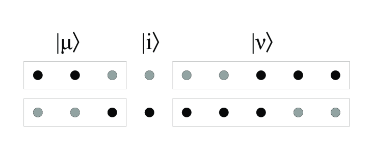
Figure 1.1: Example of MPS. $|\mu\rangle$ and $|\nu\rangle$ are Schmidt vectors from the decompositions at the sides of place $i$.

In this way, unitary operations applied on pairs of neighbour sites do not affect all the Schmidt decompositions. This suggests that Schmidt vectors can form a basis suitable for state description, one in which the process of state updating is efficient. To see how Schmidt vectors can be used, suppose that the chain is in a pure state. To see how the state can be written in matrix product state (MPS) representation, let us focus on one site of the chain. Initially, in order to describe the state, we use, on the one hand, a local representation for such a site, say $|i\rangle$, given in a standard basis, for instance spin orientation or occupation number, on the other hand, to describe the state outside this site, we use Schmidt vectors obtained from splitting the system to both sides of the place in consideration (figure 1.1). So, making explicit reference to a local basis at site $n$ the quantum state reads,

$$|\psi\rangle=\sum_{\mu\nu i}\lambda_{\mu}^{[n-1]}\lambda_{\nu}^{[n]}\Gamma_{\mu\nu}^{[n]i}|\mu\rangle^{[1,n-1]}|i\rangle^{[n]}|\nu\rangle^{[n+1,N]}.$$ (1.11)

In this way written, the quantum state appears as a superposition of states in the basis of the Schmidt vectors and the local basis of site $n$. We have deliberately specified the Hilbert spaces of every ket as a superscript. Tensor $\Gamma_{\mu\nu}^{i[n]}$ contains the components that describe the state in the new basis while coefficients $\lambda_{\mu,\nu}$ are just the Schmidt coefficients, necessary in this case to guarantee that vectors $|\mu\rangle$ and $|\nu\rangle$ are normalized.

One important property of this tensor decomposition is that it is actually possible to establish a relation among the $\Gamma$’s and the Schmidt vectors via induction. Indeed, vectors $|\nu\rangle$ can be expanded in terms of a basis $|j\rangle^{[n+1]}$ and Schmidt vectors $|\xi\rangle^{[n+2,N]}$ in this way,

$$|\nu\rangle^{[n+1,N]}=\sum_{j\xi}\Gamma_{\nu\xi}^{[n+1]j}\lambda_{\xi}^{[n+1]}|j\rangle^{[n+1]}|\xi\rangle^{[n+2,N]}$$ (1.12)

In fact, according to [21], $|\mu\rangle$ and $|\nu\rangle$ can be written in terms of the state tensors associated with the subsets $[1,...,n-1]$ and $[n+1,...,N]$ and the standard basis in the following form,

$$|\mu\rangle^{[1,n-1]}=\sum_{\alpha,...,\kappa}\left(\sum_{i_{1},...,i_{n-1}}\Gamma_{1\alpha}^{[1]i_{1}}\lambda_{\alpha}^{[1]}...\Gamma_{\kappa\mu}^{[n-1]i_{n-1}}|i_{1},...,i_{n-1}\rangle\right),$$ (1.13)

and,

$$|\nu\rangle^{[n+1,N]}=\sum_{\gamma,...,\omega}\left(\sum_{i_{n+1},...,i_{N}}\Gamma_{\nu\gamma}^{[n+1]i_{n+1}}...\lambda_{\omega}^{[N-1]}\Gamma_{\omega 1}^{[N]i_{N}}|i_{n+1},...,i_{N}\rangle\right),$$ (1.14)

where $N$ is the number of sites in the chain. Additional relations can be derived, in particular we would like to mention that the standard coefficients can be put in terms of the coefficients of the decomposition in the following way,

$$c_{i_{1},i_{2},...,i_{N}}=\sum_{\alpha,\beta,...,\omega}\Gamma_{1\alpha}^{[1]i_{1}}\lambda_{\alpha}^{[1]}\Gamma_{\alpha\beta}^{[2]i_{2}}...\lambda_{\omega}^{[N-1]}\Gamma_{\omega 1}^{[N]i_{N}}.$$ (1.15)

These coefficients enable us to write the quantum state back in the conventional basis,

$$|\psi\rangle=\sum_{i_{1},i_{2},...,i_{N}}c_{i_{1},i_{2},...,i_{N}}|i_{1},i_{2},...,i_{N}\rangle,$$ (1.16)

so that the representation of the state in terms of Schmidt coefficients and tensors, to which we refer to as canonical decomposition, fully characterizes the quantum state.

The canonical decomposition is very convenient to study numerically the time evolution of the chain. Every time that a semi-local unitary operation as in equation (1.10) is applied, the canonical representation is to be updated only for the elements involved directly with the transformation. For example, if a unitary transformation is applied on sites $4$ and $5$, we can see that for instance $\Gamma_{\mu\nu}^{[7]i_{7}}$ does not need to be updated, since the topology of the decompositions associated with the tensor, namely those in which $|\mu\rangle^{[1,6]}$ and $|\nu\rangle^{[8,N]}$ are involved, is not affected by the operation. For the case of vectors $|\mu\rangle^{[1,6]}$ particularly, a unitary operation on sites $4$ and $5$ induce a change on every vector, but the new vectors are Schmidt vectors of the evolved state with the same Schmidt coefficients. So, the new Schmidt decomposition preserves exactly the same configuration of elements with exactly the same coefficients of the initial decomposition. Therefore, no change takes place on the elements of the decomposition in places far away from where the semi-local unitary transformation operates. Following the same analysis one can establish that a unitary operation on two neighbour sites $n$ and $n+1$ generates changes only in $\Gamma^{[n]}$, $\Gamma^{[n+1]}$ and $\lambda^{[n]}$. This property constitutes the basis of efficient simulation: as the cost of updating the state depends only on the local characteristics of the system, numerical routines of low memory consumption and fast execution can be implemented using the canonical decomposition. Crucially, the factor that determines the speed of the simulation is the number of Schmidt vectors in the single value decomposition. Systems with few vectors can be updated through relatively few computational steps [22, 63]. Moreover, the canonical decomposition is also known as matrix product states (MPS) representation, and extensive documentation can be found under this denomination [26]. To see how the canonical decomposition can be updated after a semi-local unitary matrix operates, let us first focus on the simplest case where a one-site unitary operation, $\hat{U}^{[n]}$, is applied on an arbitrary site $n$. In this case we can use the expression in equation (1.11) to apply the transformation directly,

$$|\psi^{\prime}\rangle=\hat{U}^{[n]}|\psi\rangle=\sum_{\mu\nu}\sum_{i}\lambda_{\mu}^{[n-1]}\lambda_{\nu}^{[n]}U_{i}^{i^{\prime}[n]}\Gamma_{\mu\nu}^{[n]i}|\mu\rangle^{[1,n-1]}|i\rangle^{[n]}|\nu\rangle^{[n+1,N]},$$ (1.17)

so that the effect of the unitary matrix is reflected only in the coefficients $\Gamma^{[n]}$. The updated canonical coefficients are identical to the originals, with only one exception,

$${\Gamma^{\prime}}_{\alpha\beta}^{[n]i}=\sum_{k}U_{i}^{k[n]}\Gamma_{\alpha\beta}^{[n]i}.$$ (1.18)

Furthermore, this transformation does not increase the number of elements necessary to describe the state and the updating procedure can be coded easily.

Let us now assume that a two-site transformation, $\hat{U}^{[n,n+1]}$, is applied. In order to carry out such operation, the state must be written with explicit reference to the local basis of sites $n$ and $n+1$. This is done by inserting (1.12) in (1.11), which results in,

$$|\psi\rangle=\sum_{\mu\nu\xi}\sum_{ij}\lambda_{\mu}\lambda_{\xi}\Gamma_{\mu\nu}^{[n]i}\lambda_{\nu}\Gamma_{\nu\xi}^{[n+1]j}|\mu\rangle|i\rangle|j\rangle|\xi\rangle.$$ (1.19)

Therefore, the updated state reads,

$$|\psi^{\prime}\rangle=\hat{U}^{[n,n+1]}|\psi\rangle=\sum_{\mu\nu\xi}\sum_{ij}\lambda_{\mu}\lambda_{\xi}U_{ij}^{i^{\prime}j^{\prime}}\Gamma_{\mu\nu}^{[n]i}\lambda_{\nu}\Gamma_{\nu\xi}^{[n+1]j}|\mu\rangle|i\rangle|j\rangle|\xi\rangle.$$ (1.20)

As discussed before, this transformation induces changes in tensors $\Gamma_{\mu\nu}^{[n]i}$, $\Gamma_{\nu\xi}^{[n+1]i}$ and $\lambda_{\nu}$ as a result of the changes generated in the Schmidt decompositions of the splitting $[1,n-1]:[n,N]$ and $[1,n]:[n+1,N]$. Consequently, the next step consists in finding the reduced density matrix of subsystem $[n+1,N]$, from which new updated Schmidt vectors can be obtained as eigenvectors:

$$\hat{\rho}^{\prime[n+1,N]}=tr_{[1,n]}|\psi^{\prime}\rangle\langle\psi^{\prime}|.$$ (1.21)

As a result of the reduction, we are left with a density matrix spanned by the local basis of site $n+1$ and Schmidt vectors $|\xi\rangle$. Crucially, the cost involved in manipulating such density matrix, that is, storage and diagonalization, is proportional to the number of Schmidt vectors in the state. In this way, the astronomical memory requirements associated with the standard basis can be avoided, as long as the number of Schmidt vectors remains small. New coefficients ${\lambda^{\prime}}_{\nu}$ can be identified as the square roots of the eigenvalues of the reduced density matrix, whose eigenvectors can be used to get the new tensor ${\Gamma^{\prime}}_{\nu\xi}^{[n+1]j}$ directly from equation (1.12). Finally, the new tensor ${\Gamma^{\prime}}_{\mu\nu}^{[n]i}$ comes from projecting the Schmidt vectors over the whole state given by equation (1.20) [21, 23].

In order to exemplify how the canonical decomposition can be used to represent the state, let us focus on a system of three qubits. Suppose that the state of the system is given by,

$$\phi=|110\rangle.$$ (1.22)

Now, if we take the first qubit and consider the other two as the rest of the system, we can see there is only one Schmidt vector to the right, namely, $|\nu\rangle=|10\rangle$. Then, using the convention introduced in equation (1.11) the state can be written as,

$$|\phi\rangle=\lambda_{1}^{[1]}\Gamma^{[1]0}_{1,1}|0\rangle|\nu\rangle+\lambda_{1}^{[1]}\Gamma^{[1]1}_{1,1}|1\rangle|\nu\rangle,$$ (1.23)

with $\lambda_{1}^{[1]}=1$ (the Schmidt coefficient) and,

$$\Gamma^{[1]0}_{1,1}=0,$$

$$\Gamma^{[1]1}_{1,1}=1.$$

Note that the sub indices of $\Gamma^{[1]}$ make reference to the Schmidt vectors to the left and right of the first site. In this case there is only one vector to the right while for the left we imagine there is an ancillary state. Similarly, for the second site we can see the Schmidt vectors to the right and left are $|\mu\rangle=|1\rangle$ and $|\nu\rangle=|0\rangle$ respectively. The state can therefore be written as,

$$|\phi\rangle=\lambda_{1}^{[1]}\lambda_{1}^{[2]}\Gamma^{[2]0}_{1,1}|\mu\rangle|0\rangle|\nu\rangle+\lambda_{1}^{[1]}\lambda_{1}^{[2]}\Gamma^{[2]1}_{1,1}|\mu\rangle|1\rangle|\nu\rangle,$$ (1.24)

with,

$$\Gamma^{[2]0}_{1,1}=0,$$

$$\Gamma^{[2]1}_{1,1}=1,$$

and $\lambda_{1}^{[2]}=1$. Finally, the coefficients of the third site can be extrapolated from,

$$|\phi\rangle=\lambda_{1}^{[2]}\Gamma^{[3]0}_{1,1}|\mu\rangle|0\rangle+\lambda_{1}^{[2]}\Gamma^{[3]1}_{1,1}|\mu\rangle|1\rangle,$$ (1.25)

with,

$$\Gamma^{[3]0}_{1,1}=1,$$

$$\Gamma^{[3]1}_{1,1}=0,$$

and as the reader may have guessed, $|\mu\rangle=|11\rangle$. In the same manner, we can obtain the canonical decomposition of the following less trivial state,

$$\phi=\frac{|001\rangle+|011\rangle}{\sqrt{2}}=|0\rangle\left\{\frac{|0\rangle+|1\rangle}{\sqrt{2}}\right\}|1\rangle.$$ (1.26)

This state can be written with explicit reference to the coordinates of the first qubit exactly as in equation (1.23), but with,

$$\Gamma^{[1]0}_{1,1}=1,$$

$$\Gamma^{[1]1}_{1,1}=0,$$

and,

$$|\nu\rangle=\left\{\frac{|0\rangle+|1\rangle}{\sqrt{2}}\right\}|1\rangle.$$ (1.27)

Similarly, the state also adopts the form of equation (1.24), but with the following important changes,

$$\Gamma^{[2]0}_{1,1}=\frac{1}{\sqrt{2}},$$

$$\Gamma^{[2]1}_{1,1}=\frac{1}{\sqrt{2}},$$

and $|\mu\rangle=|0\rangle$ and $|\nu\rangle=|1\rangle$. Likewise, it can be seen that for the third site the coefficients of equation (1.25) are given by,

$$\Gamma^{[2]0}_{1,1}=0,$$

$$\Gamma^{[2]1}_{1,1}=1,$$

and the Schmidt vector is,

$$|\mu\rangle=|0\rangle\left\{\frac{|0\rangle+|1\rangle}{\sqrt{2}}\right\}.$$ (1.28)

More complex representations can be derived when there are partitions with more than one Schmidt vector in the decomposition. We hope that these simple examples allow the reader to grasp an idea about the mechanics associated with writing a quantum state using MPS.

1.4 Perfect transmission hopping

In a chain of bosons with constant chemical potential and zero repulsion the Hamiltonian can be written as,

$$\hat{H}=\sum_{k=1}^{N-1}{J_{k}(\hat{a}^{\dagger}_{k+1}\hat{a}_{k}+\hat{a}^{\dagger}_{k}\hat{a}_{k+1})},$$ (1.29)

where $\hat{a}_{k}^{\dagger}$ and $\hat{a}_{k}$ are the usual bosonic operators with standard commuting rules, namely,

$$[\hat{a}_{k},\hat{a}_{l}]=0,\hskip 14.22636pt\left[\hat{a}^{\dagger}_{k},\hat{a}^{\dagger}_{l}\right]=0,\hskip 14.22636pt\left[\hat{a}_{l},\hat{a}^{\dagger}_{k}\right]=\delta_{k}^{l},$$ (1.30)

and $N$ is the number of sites in the chain. One question of interest in several branches of physics is whether it is possible to dynamically transfer an arbitrary quantum state from one end of the chain to the other with maximum fidelity. In other words, whether it is possible to have a perfect transmission channel. This problem has been extensively studied and here we limit ourselves to outline the main results of more specialized investigations presented elsewhere [64, 65, 66, 67, 68]. Perfect transmission was first studied in spin chains due to the interest prompted by the novel scheme shown in reference [43]. In this reference, spin chains were proposed as alternative channels to transfer quantum information encoded in the state of the spins. In this context, it became important to know under which specific circumstances a spin chain could transmit a state without the state being corrupted by the underlying dynamics. It turned out that chains with constant coefficients could be used as efficient transmission channels only in chains of maximum 3 sites. However, it was also found that chains with variable hopping coefficients could be made efficient if the right hopping coefficients were chosen. Such coefficients could be identified by noticing the parallel between the dynamics of the chain and the physics of the angular momentum. In this analogy, states on the ends of the chain correspond to eigenstates of angular momentum with large eigenvalues, while states in the centre turn out to be analogous to eigenvectors associated with the smallest eigenvalues. It was shown that in a system governed by Hamiltonian (1.29) perfect transmission can be accomplished by choosing what we call perfect transmission hopping (PTH),

$$J_{k}^{PTH}=\frac{\lambda}{2}\sqrt{k(N-k)},$$ (1.31)

where $\lambda$ is a constant that fixes the time scale (for simplicity we chose $\lambda=2$ for numerical simulations). This stands in contrast to the widely used constant hopping (CH), given simply by,

$$J_{k}^{CH}=1.$$ (1.32)

When inserted in Hamiltonian (1.29), PTH induces a mirror-reflection of the initial state with respect to the chain centre at a time,

$$t=\frac{T}{2}=\frac{\pi}{\lambda}.$$ (1.33)

This property constitutes the basis of perfect state transmission between the chain terminals. Independently of how many bosons initially occupy either chain end, they all turn up at the opposite end in a PTH chain with all repulsion constants set to zero [52].

Although the dynamics of a PTH chain with no repulsion has been already studied, there are several research extensions of interest. On the one hand, it is important to know if chains with variable hopping coefficients and repulsion can display perfect transmission. If they cannot, it would be interesting to know how the repulsion hampers the state transmission. Similarly, if transmission with repulsion is possible, it would be important to know the specific circumstances under which this phenomenon can be observed. Works on this direction have produced very interesting results [67]. In addition to these research areas, here we also focus on one alternative approach. In fact, in sections ahead we intend to see the problem from a rather different perspective. Certainly, it is quite valid to ask how PTH affects physical phenomena in which transport does not participate straightforwardly. From our viewpoint, this constitutes an important aspect to study in chains with efficient transmission, as the regularities of the Hamiltonian that lead to perfect transmission could give rise to interesting coherent processes. Similarly, it should be mentioned that very promising experimental proposals to realize PTH in optical lattices have been discussed in reference [68] by the same group that proposed the realization of the Hubbard model in optical latices. Therefore, such kind of hopping profile should be considered as a feasible alternative and not just as a theoretical idealization.

Chapter 2 Implementation and numerics

The first aspect to be handled when addressing the construction of a program using the formalism presented in previous sections, is memory allocation. It is indeed possible to implement the algorithm using standard programming tools, that is, vectors and matrices with permanent memory attributes. However, the way in which the elements of the canonical decomposition depend on the Schmidt vectors makes the canonical tensors vary in size according to the number of Schmidt vectors in the decomposition. Therefore, it is preferable to adopt a programming style in which the dynamical nature of the algorithm can be handled more appropriately. FORTRAN 95 offers several tools that can be conveniently adjusted to approach the dynamical nature of the method. On the one hand, it allows one to actually define the geometry of the objects employed to store data. This means that in addition to vectors and matrices, tensors of whatever shape and dimension can be used. For instance, we can define a vector in which every component is a matrix, or a matrix in which every element is made of a complex number and a real vector. The other tool is dynamical allocation. The elements that we use to store numbers are not necessarily fixed in size, instead, we can make them bigger or smaller according to the simulation requirements. In FORTRAN 95, dynamical allocation can be implemented using either allocatable objects or pointers. Pointers work very much as allocatable objects, but they have two useful additional properties. First, they can be alternatively used as aliases of other objects, and second, they can be passed from one routine to another as arguments. Modules are another useful tool. Variables defined in a module can be used in any routine by just including the module in the routine’s headlines. In our program for example, the module bskt contains the tensors of the canonical decomposition. In order to define an object such as $\lambda_{\alpha}$, we must first generate the type that supports the object. This is done through the lines,

type dl
real(dp), dimension(:), pointer :: ld
end type dl

Tensor $\lambda_{\alpha}$, is then written as an element defined by the rules of type dl,

type(dl), dimension(N) :: LAM

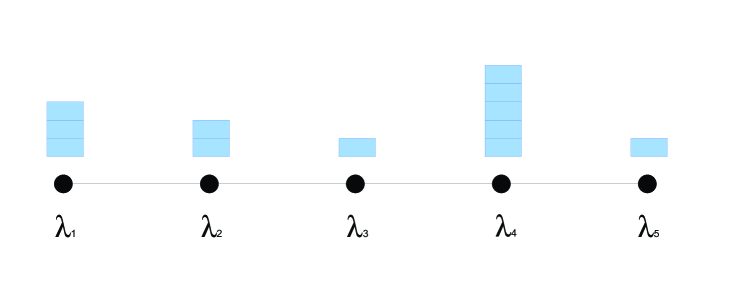
Figure 2.1: Sketch of memory allocation of LAM(i)%ld

This means that there is one pointer associated to every site of the chain. Each pointer is independent and can be given whatever memory one needs to allocate (figure 2.1). So, if for example the Schmidt decomposition in site 5 has 3 coefficients, then in order to allocate that specific amount of space we write,

allocate(LAM(5)%ld(3))

and then proceed to specify every component of LAM(5)%ld. Similarly, tensor $\Gamma_{\alpha\beta}^{[n]i}$ is an object that can be allocated in two dimensions, namely those associated with $\alpha$ and $\beta$. Every component of this allocatable arrangement, on the other hand, is a complex vector of fixed size. The components of such vectors correspond to a local basis, in this case given in terms of the label $i$, whose maximum value is set to be $M$. Therefore, we must utilize two types to define the variable, namely,

type fg
complex(dpc), dimension(M) :: gf
end type fg

type dg
type(fg), dimension(:,:), pointer :: gd
end type dg

the variable itself is defined the same way as LAM was defined before,

type(dg), dimension(N) :: GAM

that is, one storage unit per site. For this variable, allocation takes place only in the pointer section. For instance,

allocate(GAM(2)%gd(3,5))

and then, if we want to give numerical values to the tensor we would write, for example,

GAM(2)%gd(1,3)%gf(2) = some complex number

In this way, no memory space is wasted through undefined memory slots. When using memory allocation, special care must be taken in processing allocatable units. If a variable is allocated, then it must be deallocated if for some reason we want to allocate it again, for example as the decomposition is updated, otherwise the memory associated with the variable will not be accessible any more and one can easily run out of virtual memory in a long simulation. The most challenging part of a time evolving block decimation (TEBD) program, is the updating routine in which a two-site unitary transformation is applied and some tensors must be worked out (figure (2.2)).

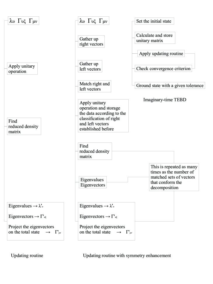
Figure 2.2: Flux diagrams.

In a program that makes use of symmetries, we must first organize the vectors of the decomposition in groups of elements sharing the same symmetry, which at the same time involves finding the symmetry of the vectors themselves. Once this is done, we apply the updating procedure to sets of vectors with complementary symmetry, in such a way that one global symmetry is preserved. Finally, the symmetry associated with the new tensors must be found and attached in order to be able to access this important information in the next run of computations. The reason why we implement symmetry enhancement is because the cost of updating the decomposition in small subspaces is lower than the one of updating all the elements at once by diagonalizing a single large matrix.

Similarly, in a problem where the quantum state is symmetric with respect to the centre of the chain, we can simulate the dynamics by updating the coefficients only on one half of the chain and extrapolating some coefficients in the middle. This involves using the fact that in a symmetric chain with an even number of sites the reduced density matrix of the two central sites has a degenerate spectrum and eigenvectors corresponding to the same eigenvalue are in fact complementary.

One additional feature of FORTRAN 95 which hugely facilitates memory management are linked lists. They basically consist in variables that can be given extra allocatable space without destroying the information already contained in the variable. Note that this is not the case for pointers, since every time that a pointer is reallocated it must be previously deallocated and so any associated content is automatically lost. A linked list can be made of any valid memory unit such as vectors, matrices, pointers and even types. In the updating routine, for instance, we use linked lists to store the Schmidt vectors as we do not know in advance how many vectors conform the decomposition of the updated state.

We also would like to comment about one element of the research with challenging numerically aspects. As it has been discussed, the calculation of entanglement in mixed states involves dealing with the density matrix. Here, such matrix comes from reducing the pure state of the whole system. In order to find the entanglement between the ends, or end-to-end entanglement (EEE), the reduced density matrix in the standard basis must be computed using the canonical coefficients. To see how the reduction takes place, let us write the quantum state of the chain in the following way [21],

$$|\psi\rangle=\sum_{\alpha_{1},\alpha_{2},...,\alpha_{N-1}}|1\alpha_{1}\rangle^{[1]}\lambda_{\alpha_{1}}^{[1]}|\alpha_{1}\alpha_{2}\rangle^{[2]}\lambda_{\alpha_{2}}^{[2]}...\lambda_{\alpha_{N-1}}^{[N-1]}|\alpha_{N-1}1\rangle^{[N]},$$ (2.1)

where,

$$|\alpha\alpha^{\prime}\rangle^{[n]}=\sum_{i}\Gamma_{\alpha\alpha^{\prime}}^{[n]i}|i\rangle.$$ (2.2)

Consequently, the reduced density matrix looks like,

$$\hat{\rho}_{1N}=$$

$$\sum_{\binom{\alpha_{1},\alpha_{2},...,\alpha_{N-1},}{{\alpha^{\prime}}_{1},{\alpha^{\prime}}_{2},...,{\alpha^{\prime}}_{N-1}}}|1\alpha_{1}\rangle^{[1]}\langle{1\alpha^{\prime}}_{1}|^{[1]}\lambda_{\alpha_{1}}^{[1]}\lambda_{{\alpha^{\prime}}_{1}}^{[1]}\langle\alpha_{1}\alpha_{2}|{\alpha^{\prime}}_{1}{\alpha^{\prime}}_{2}\rangle^{[2]}\lambda_{\alpha_{2}}^{[2]}\lambda_{{\alpha^{\prime}}_{2}}^{[2]}\langle\alpha_{2}\alpha_{3}|{\alpha^{\prime}}_{2}{\alpha^{\prime}}_{3}\rangle^{[3]}...$$

$$...\langle\alpha_{N-2}\alpha_{N-1}|{\alpha^{\prime}}_{N-2}{\alpha^{\prime}}_{N-1}\rangle^{[N-1]}\lambda_{\alpha_{N-1}}^{[N-1]}\lambda_{{\alpha^{\prime}}_{N-1}}^{[N-1]}|\alpha_{N-1}1\rangle^{[N]}\langle{\alpha^{\prime}}_{N-1}1|^{[N]}$$ (2.3)

$$=\sum_{\alpha_{1},{\alpha^{\prime}}_{1},\alpha_{N-1},{\alpha^{\prime}}_{N-1}}|1\alpha_{1}\rangle^{[1]}\langle{1\alpha^{\prime}}_{1}|^{[1]}M_{\{\alpha_{1}\alpha_{N-1}\}\{{\alpha^{\prime}}_{1}{\alpha^{\prime}}_{N-1}\}}|\alpha_{N-1}1\rangle^{[N]}\langle{\alpha^{\prime}}_{N-1}1|^{[N]}.$$

Most of the programming work is devoted to write matrix $M_{\{\alpha_{1}\alpha_{N-1}\}\{{\alpha^{\prime}}_{1}{\alpha^{\prime}}_{N-1}\}}$ in a way that can be efficiently stored and manipulated. The storage matter is related to conservation properties. In the case of $\hat{\rho}_{1N}$, conservation splits the operator in representations holding $S_{\alpha_{1}}+S_{\alpha_{N-1}}=S_{{\alpha^{\prime}}_{1}}+S_{{\alpha^{\prime}}_{N-1}}$, where $S_{\alpha}$ is the symmetry associated with ket $|\alpha\rangle$. The same splitting applies for $M_{\{\alpha_{1}\alpha_{N-1}\}\{{\alpha^{\prime}}_{1}{\alpha^{\prime}}_{N-1}\}}$. In order to compute this matrix, one first calculates the products $\lambda_{\alpha_{1}}^{[1]}\lambda_{{\alpha^{\prime}}_{1}}^{[1]}\langle\alpha_{1}\alpha_{2}|{\alpha^{\prime}}_{1}{\alpha^{\prime}}_{2}\rangle^{[2]}$ and creates a temporary support matrix $M_{\{\alpha_{1}\alpha_{2}\}\{{\alpha^{\prime}}_{1}{\alpha^{\prime}}_{2}\}}$. This computation can be accelerated by exploiting the fact that in a state like (2.2) a symmetry restriction bounds the indices through

$$S_{\alpha}+S_{\alpha^{\prime}}+S_{i}=S_{\text{Global Simmetry}},$$ (2.4)

therefore, to compute an inner product such as,

$$\langle\alpha\alpha^{\prime}|\beta\beta^{\prime}\rangle,$$ (2.5)

one just takes the indices in the kets and finds the corresponding local coordinate $i$ using equation (2.4). Only if the coordinates coincide the associated contribution is stored using linked lists. In the next run of computations, for every pair of indices $\alpha_{3},{\alpha^{\prime}}_{3}$ one sweeps over the range of values of the indices $\alpha_{2},{\alpha^{\prime}}_{2}$ and finds the product $\lambda_{\alpha_{2}}^{[2]}\lambda_{{\alpha^{\prime}}_{2}}^{[2]}\langle\alpha_{2}\alpha_{3}|{\alpha^{\prime}}_{2}{\alpha^{\prime}}_{3}\rangle^{[3]}$. Again, only if the inner product is not zero the contribution is added up. After this is completed, we are left with a support matrix $M_{\{\alpha_{1}\alpha_{3}\}\{{\alpha^{\prime}}_{1}{\alpha^{\prime}}_{3}\}}$. The process goes on until we finally get the matrix with the end indices.

Improved performance can be achieved if spatial symmetry is taken into consideration. This is done in a very similar way than with the canonical coefficients, that is, when the computations come to the middle of the chain, we group up complementary representations from each side of the chain and perform our operations in subspaces, always keeping the total number of bosons fixed.

Once the reduced density matrix for the chain terminals has been worked out, we use it to calculate the logarithmic negativity. This involves performing a series of rearrangement operations, as for example, the explicit calculation of the partial transpose matrix. This process alone carries a technical issue of particular trickiness that we want to comment about. As we already pointed out, the conservation of the total number of particles allows us to split large matrices into several smaller representations that we can manage more easily. As a consequence, what we call reduced density matrix is actually a set of matrices, each one corresponding to a different quantum number. This can be understood by thinking that every matrix matches a state of the chain with a complementary quantum number. Therefore, there are as many matrices as number of bosons plus one, as the no-boson possibility must be accounted for too. The splitting is not only practical but often necessary, because the amount of information that we can handle using a computer is limited. Nevertheless, this splitting may be broken if the state is subject to non-unitary transformations. This is precisely what happens when we try to compute the partial transpose. As a matter of fact, the transposition operation mixes subspaces with different quantum numbers. The good news is that the transpose matrix keeps some kind of regularity that allows us to split the matrix into non-interacting subspaces that we can address individually. Hence, before starting with the operations that determine the new matrix, we first establish the subspaces that conform the new splitting, and then proceed to fill every conforming matrix with the corresponding elements. Once this is completed, finding the eigenvalues and computing the logarithmic negativity from equation (1.8) is straightforward.

These are the numerical issues that in our opinion require special care and analysis before they can be efficiently implemented in a program. Even though these aspects of our investigation do not shed by themselves any physical insight, we have decided to include this discussion as a way of presenting a complete view of the problem as well as its collateral issues.

Chapter 3 Matrix product states in ideal boson chains

In a boson chain of $N$ sites and $M$ bosons in which particle exchange can potentially take place among any two places, the Hamiltonian of the system reads,

$$\hat{H}=\sum_{k=1}^{N}R_{k,k}\hat{a}^{\dagger}_{k}\hat{a}_{k}+\sum_{k=1}^{N}\sum_{l=k+1}^{N}{\left(R_{k,l}\hat{a}^{\dagger}_{k}\hat{a}_{l}+{R^{*}}_{k,l}\hat{a}^{\dagger}_{l}\hat{a}_{k}\right)}$$ (3.1)

In such a way that $R_{k,l}$ represents the strength of the hopping between sites $k$ and $l$. The creation $\hat{a}_{k}^{\dagger}$ and annihilation $\hat{a}_{k}$ operators follow the standard commuting rules for a discrete model given by equation (1.30).

The Hamiltonian above is quadratic and can be decoupled in order to get the ground state. Additionally, the Heisenberg equations of motion for the creation operators produce a complete set of differential equations that can be written as,

$$\frac{d}{dt}\left(\begin{array}[]{c}\hat{\alpha}_{1}\\ \hat{\alpha}_{2}\\ \hat{\alpha}_{3}\\ \vdots\\ \hat{\alpha}_{N}\\ \end{array}\right)=-i\left(\begin{array}[]{ccccc}R_{1,1}&R_{1,2}&R_{1,3}&\cdots&R_{1,N}\\ {R^{*}}_{1,2}&R_{2,2}&R_{2,3}&\cdots&R_{2,N}\\ {R^{*}}_{1,3}&{R^{*}}_{2,3}&R_{3,3}&\cdots&R_{3,N}\\ \vdots&\vdots&\vdots&\ddots&R_{N-1,N}\\ {R^{*}}_{1,N}&{R^{*}}_{2,N}&{R^{*}}_{3,N}&{R^{*}}_{N-1,N}&R_{N,N}\\ \end{array}\right)\left(\begin{array}[]{c}\hat{\alpha}_{1}\\ \hat{\alpha}_{2}\\ \hat{\alpha}_{3}\\ \vdots\\ \hat{\alpha}_{N}\\ \end{array}\right),$$ (3.2)

or equivalently,

$$\frac{d\mbox{ \boldmath$\hat{\alpha}$ }}{dt}=-i\hat{R}\mbox{\boldmath$\hat{\alpha}$},$$ (3.3)

where $\hat{\alpha}_{k}$ describes the corresponding creation operator in the Heisenberg picture,

$$\hat{\alpha}_{k}=e^{-it\hat{H}}\hat{a}^{\dagger}_{k}e^{it\hat{H}}.$$ (3.4)

These equations are complemented by the initial conditions,

$$\hat{\alpha}_{k}(t=0)=\hat{a}_{k}^{\dagger}.$$ (3.5)

The state, on the other hand, is given in terms of the Heisenberg operators by,

$$|\psi(t)\rangle=\frac{1}{\sqrt{\prod_{j}^{N}n_{j}!}}\prod_{k}^{N}\hat{\alpha}_{k}^{n_{k}}|0\rangle.$$ (3.6)

The way in which particles are distributed across the chain is determined by the constants $n_{j}$.

From equation (3.3) it is in fact possible to obtain the ground state of the system through imaginary time analysis (equation (4.7)). In doing so, the ground state is found to be,

$$|G\rangle=\left(\sum_{k=0}^{N}c_{k}\hat{a}^{\dagger}_{k}\right)^{M}|0\rangle,$$ (3.7)

where coefficients $c_{k}$ are the components (possibly complex) of the ground eigenvector of matrix $\hat{R}$, so that,

$$\sum_{k=1}^{N}|c_{k}|^{2}=1.$$ (3.8)

From equation (3.7) we can extract some information. Nevertheless, because the description of the state demands exponentially growing resources which scale with both $N$ and $M$, calculations involving non-local correlations can be fairly challenging. In order to set state (3.7) in a way that can be easily handled, we will apply unitary operations to the state so as to simplify it as much as possible. The idea is to reduce $|G\rangle$ to an expression that can be written using MPS. Then, if the unitary operations only involve transformation to first neighbours, the updating method presented in previous sections can be applied. This would provide us with a complete description of the state that we can efficiently use.

We first operate locally on individual sites using the transformation,

$$\hat{U}_{k}^{(1)}=e^{-i\theta_{k}\hat{a}_{k}^{\dagger}\hat{a}_{k}}.$$ (3.9)

In this equation $\theta_{k}$ is the phase of the complex number $c_{k}$. As a result of this transformation we get,

$$\hat{a}_{k}^{\dagger}\rightarrow e^{-i\theta_{k}}\hat{a}_{k}^{\dagger}.$$ (3.10)

In such a way that the complex phase is cancelled out. Additionally, any operator different from $\hat{a}_{k}$ remains unaffected by the transformation. Once this has been done for every operator $\hat{a}_{k}$, the new coefficients $c_{k}$ in equation (3.2) are real.

Subsequently, we apply unitary operations involving first neighbours in the following fashion,

$$\hat{U}_{k}^{(2)}=e^{-i\phi_{k}\left(\frac{1}{2i}(\hat{a}_{k+1}^{\dagger}\hat{a}_{k}-\hat{a}_{k}^{\dagger}\hat{a}_{k+1})\right)}=e^{-i\phi_{k}\hat{Q}_{k}}.$$ (3.11)

In physical terms, operator $\hat{Q}_{k}$ is known as the current, and its eigenvalues indicate how many bosons circulate in between sites $k$ and $k+1$. As a result of this unitary operation, the pair $\{\hat{a}_{k}^{\dagger},\hat{a}_{k+1}^{\dagger}\}$ transforms as,

$$c_{k+1}\hat{a}_{k+1}^{\dagger}+c_{k}\hat{a}_{k}^{\dagger}\rightarrow$$ (3.12)

$$\left(c_{k+1}\cos\left(\frac{\phi_{k}}{2}\right)-c_{k}\sin\left(\frac{\phi_{k}}{2}\right)\right)\hat{a}_{k+1}^{\dagger}+\left(c_{k+1}\sin\left(\frac{\phi_{k}}{2}\right)+c_{k}\cos\left(\frac{\phi_{k}}{2}\right)\right)\hat{a}_{k}^{\dagger}.$$

Therefore, we can cancel operator $\hat{a}_{k+1}^{\dagger}$ by just choosing an angle $\phi_{k}$ satisfying,

$$\tan\left(\frac{\phi_{k}}{2}\right)=\frac{c_{k+1}}{c_{k}}.$$ (3.13)

Consequently, in order to reduce the state to one single mode operating on the vacuum, we apply the operations (3.11), starting from $k=N-1$, to every couple of consecutive operators. Note that every time a transformation acts on any pair of modes, the coefficient that accompanies the creation operator that is not taken out is affected, but it always remains real.

When the reduction is completed, we are left with a state as (up to an overall constant),

$$|g\rangle=\frac{1}{\sqrt{M!}}\left(\hat{a}_{1}^{\dagger}\right)^{M}|0\rangle,$$ (3.14)

which can be easily written using MPS. The next step consists in applying the inverse operations in reverse order to the state using the method presented in section 1.3. From now on, we will refer to this reduction operation as state folding.

There is also the case when we must deal with numerous summations acting on the vacuum. For instance, in chains with an initial state given by bosons arranged on different positions. In this kind of situation state folding can be utilized too. Let us consider the case when just two summations get involved so that the state reads,

$$\left(\overbrace{\sum_{k=1}^{N}c_{k}\hat{a}_{k}^{\dagger}}^{S_{2}}\right)^{M_{2}}\left(\overbrace{\sum_{l=1}^{N}z_{l}\hat{a}_{l}^{\dagger}}^{S_{1}}\right)^{M_{1}}|0\rangle,$$ (3.15)

where $M_{1}$ is the number of bosons originally allocated on one site of the chain and $M_{2}$ has an analogous meaning. We can use the standard technique to fold $S_{1}$, but it is worth saying that in the process the coefficients of $S_{2}$ are also affected. Next, we can fold the new $S_{2}$ from $\hat{a}_{N}^{\dagger}$ just until $\hat{a}_{2}^{\dagger}$, since folding $\hat{a}_{2}^{\dagger}$ in $S_{2}$ would unfold $S_{1}$. As a result, the folded state must be written making explicit reference to such last folding operation in the form,

$$|g\rangle=\left(\hat{a}_{1}^{\dagger}\right)^{M_{2}}e^{-i\phi_{1}\hat{Q}_{1}}\left(\hat{a}_{1}^{\dagger}\right)^{M_{1}}|0\rangle.$$ (3.16)

Consequently, $|g\rangle$ can be written in MPS by first translating $|M_{1},0,...,0\rangle$ into MPS and then applying $e^{-i\phi_{1}\hat{Q}_{1}}$. In this way, we are left with a canonical decomposition that can be used to apply the last operation in the row. With this in mind we set down the state with explicit reference to the local coordinates of the first position and then apply $\left(\hat{a}_{1}^{\dagger}\right)^{M_{2}}$ in a very straightforward way. In doing so we get,

$$|g\rangle=\sum_{\gamma=1}^{N_{\gamma}}\Gamma_{1\gamma}^{[1]j}\lambda_{\gamma}^{[1]}\sqrt{(j+M_{2})!}|j+M_{2}\rangle|\gamma\rangle^{[2-N]}.$$ (3.17)

In latter equation we have made use of the fact that the number of bosons in the local basis of the first site $|j+M_{2}\rangle$ is determined by the number of bosons in the complementary Schmidt vector $|\gamma\rangle$ and therefore there is only one relevant coordinate that describes the local basis. This explains the lack of a summation symbol for the label $j$. From the expression above the canonical coefficients of state $|g\rangle$ can be directly obtained, namely,

$${\lambda^{\prime}}_{\gamma}^{[1]}=\sqrt{(j+M_{2})!}\lambda_{\gamma}^{[1]}+\text{normalization},$$ (3.18)

$${\Gamma^{\prime}}_{1\gamma}^{[1]j+M_{2}}=\Gamma_{1\gamma}^{[1]j}.$$ (3.19)

However, because this is not a unitary transformation, it is important to show that the canonical decomposition obtained in this way is consistent. It is not difficult to see that the canonical tensors attached from the third site onwards do not suffer any modification whatsoever since this section of the chain is made of complementary partitions which contain only one Schmidt vector. This is because there is no boson at all between the third and the last position. We can see that such is indeed the case by noticing that the operations performed on the vacuum involved only the first and second places, thereby only these two positions can hold any non-vanishing population. On the other hand, we know that the tensor elements in positions one and two depend directly on the Schmidt vectors $\{|\gamma_{i}\rangle^{[1]}\}$. These vectors all have well defined quantum numbers on account of particle conservation. Therefore, when we apply $\left(\hat{a}_{1}^{\dagger}\right)^{M_{2}}$ we are actually lifting the boson occupation which means that the resulting vectors are valid Schmidt vectors which are orthogonal to each other.

3.1 Quench in trapped systems

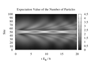
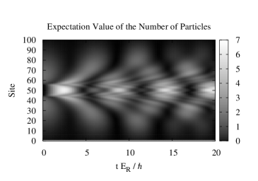
Figure 3.1: Expectation value of the number of particles. Top plots are grey maps of the lower plots. Dynamics is generated by turning a potential barrier in the middle on (left) and off (right).

We now show how the method presented in the previous section is capable of delivering results in challenging scenarios. In what follows, we assume that energy is given in terms of the recoil energy,

$$E_{R}=\frac{\hbar k^{2}}{2m},$$ (3.20)

where $k$ is the wavelength of the confining laser and $m$ is the atomic mass. Let us consider a chain of 100 sites and 100 bosons which has been cooled down to the ground state in the presence of a trapping potential given by,

$$R_{i,i}=\Omega(i-50)^{2},$$ (3.21)

with $\Omega=0.00046E_{R}$, a reasonable experimental factor according to reference [39]. Additionally, we assume that particle exchange can take place among any two places in the chain, not only next neighbours. The intensity of the hopping is proportional to the off-diagonal matrix elements,

$$R_{i,j}=\frac{\Xi}{|i-j|},$$ (3.22)

for every $i\neq j$ and with $\Xi=0.3E_{R}$. This choice of hopping can be justified in chains with long-range exchange effects, such as expected in situations where the Coulomb potential plays an important role. In a first set of simulations, we find the ground vector of matrix $\hat{R}$ and insert the coefficients in equation (3.7). Dynamics is generated by instantaneously turning on (off) a very high potential barrier in the middle of the chain. This barrier is written as,

$$R_{i,i}=1000E_{R}\hskip 14.22636pt\text{for}\hskip 14.22636pt45<i<55.$$ (3.23)

Next, we find the ground state of the system including the potential barrier so as to generate a distribution with two condensates at the sides of the wall and then turn the potential barrier off. Figure 3.1 shows the behaviour of the expectation value of the number of bosons for the above mentioned configurations. As a result of the quench very characteristic wave patterns are generated depending on how the quench takes place. In both cases, however, fleeing waves are generated after a particle bulk assembles in the chain centre. In the first case, when the barrier is turned on before the condensate is released, we can see that a large part of the condensate remains in the middle of the chain, just where the barrier stands. The barrier domain seems to determine a zone from which bosons can hardly escape. It is reasonable as the high potential difference between sites inside and outside the wall zone energetically hinders any quantum jump. In contrast, the pattern generated in the case when the dynamics is generated by switching the potential barrier off is more compatible with uniform expansion. Nevertheless, in both cases we can appreciate the effect of the inclusion of long range hopping terms in the Hamiltonian. When the bosonic waves travel outwards they gradually lose particles. However, this loss does not translate in dissipation, instead, a new boson bulk reassembles around the centre of the chain and a new expansion starts again. This effect is clearer in the case of expansion without intermediate potential, but it also takes place in the other case analysed. Such profile is in contrast with the behaviour of travelling packets of chains with next-neighbour hopping only. In the latter case the changes in the form of the wave pattern develop locally around the boson bulk, and the effect of particle exchange between distant places of the chain is much less pronounced.

3.2 Entanglement as a result of collision

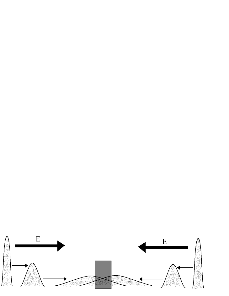
Figure 3.2: Sketch of a bosonic collision

In this section we want to show how the two-sum folding method can be used in time dependent problems. Let us suppose that in a boson chain we have two very well localized boson clouds at the ends. We then use a physical mechanism to accelerate the clouds and make them interact with each other. After this collision process, the scattered bosons are collected and taken back to the chain terminals. Because of the interaction between the boson packets, the collected particles at the ends are strongly entangled, as discussed in [69, 70, 71, 72]. Certainty, this entanglement would be potentially useful for multiple quantum information procedures. Before focusing on entanglement, however, we will look at how the bosons get transmitted from one end of the chain to the other in the presence of a perturbation in the central part. In such a system the Hamiltonian would be ideally given by equation (3.1) with a matrix $\hat{R}$ that can be written as,

$$\hat{R}=\hat{J}_{x}+\epsilon e^{-\beta\hat{J}_{z}^{2}},$$ (3.24)

where $\hat{J}_{x,y,z}$ are the standard angular momentum operators. $\epsilon$, on the other hand, represents the intensity of a symmetrically localized perturbation in the middle of the chain and $\beta$ measures the spread of such perturbation. One reason to put matrix $\hat{R}$ in terms of the angular momentum operators is that in this way we can highlight the analogy between perfect transmission in a boson chain and the physics of angular momentum. In fact, in the absence of a term proportional to $\epsilon$, this would be basically a particle spinning around the x-axis. The perturbation has been deliberately chosen in the form of an exponential in order to generate a decaying profile as going from the middle of the chain towards the terminals. This form is also very convenient to perform analytical calculations as we will show. In addition to this formulation of matrix $\hat{R}$, we must establish a relation among the state kets in the Hilbert space and the actual operators. This can be worked out by just comparing the effect of the angular momentum on the corresponding kets with the predicted behaviour of the operators in the perfect transmission scenario. From this we can infer,

$$|j,m\rangle\rightarrow\hat{a}_{j-m+1}^{\dagger}.$$ (3.25)

In this expression we used the standard notation for the angular momentum kets, that is, $|j,m\rangle$ are the eigenstates of the z-component operator $\hat{J}_{z}$. The quantum number $j$ is related to the total number of sites in the chain by the identity,

$$j=\frac{N-1}{2}.$$ (3.26)

In this way, the evolution of the Heisenberg operators can be studied by following the dynamics of the associated kets. In a problem where the physics of the system is dictated by equation (3.24) the wave function acquires the following form after half a period evolution,

$$|\psi(t=\pi)\rangle=e^{-i\pi(\hat{J}_{x}+\epsilon e^{-\beta\hat{J}_{z}^{2}})}|j,j\rangle.$$ (3.27)

Here we have implicitly assumed that the length of the angular momentum $j$ is an arbitrary integer which accounts for $N$ being odd. We have focused on the evolution of $|j,j\rangle$ because that is the ket relevant to operator $\hat{a}_{1}$ and therefore the one which contains information about the transmission of bosons initially prepared on the first site of the chain. Making use of time dependent perturbation theory we can expand the latter expression in the following way,

$$|\psi(t=\pi)\approx e^{-i\pi\hat{J}_{x}}|j,j\rangle-i\epsilon|\epsilon\rangle,$$

$$|\epsilon\rangle=\int_{0}^{\pi}dte^{-i(\pi-t)\hat{J}_{x}}e^{-\beta\hat{J}_{z}^{2}}e^{-it\hat{J}_{x}}|j,j\rangle,$$ (3.28)

of course, this approximation holds as long as the amplitude of the dynamics generated by the integral in the second term remains small compared to the unperturbed evolution. For this to happen it is important not only that $\epsilon$ is a little fraction but also that the dynamics develops out of resonance. Nevertheless, in this particular case where we restrict ourselves to well defined time intervals, the emergence of cooperative resonances is quite improbable. So, the integral above can be manipulated as,

$$|\epsilon\rangle=\int_{0}^{\pi}dte^{-i(\pi-t)\hat{J}_{x}}e^{-\beta\hat{J}_{z}^{2}}e^{i(\pi-t)\hat{J}_{x}}e^{-i\pi\hat{J}_{x}}|j,j\rangle.$$ (3.29)

From the properties of the angular momentum we know

$$e^{-i\pi\hat{J}_{x}}|j,j\rangle=|j,-j\rangle.$$ (3.30)

Further simplifications apply by noticing that the three first exponentials from left to right underline a unitary transformation. As a result we can write,

$$|\epsilon\rangle=\int_{0}^{\pi}dte^{-\beta(\cos(t)\hat{J}_{z}-\sin(t)\hat{J}_{y})^{2}}|j,-j\rangle.$$ (3.31)

Because the operator on the integral is squared, we do not have a way to translate the expression into a sum of kets. Therefore, we rather use the well known result from integral calculus,

$$\int_{-\infty}^{\infty}dxe^{-(ax^{2}+bx)}=\sqrt{\frac{\pi}{a}}e^{\frac{b^{2}}{4a}},$$ (3.32)

to put $|\epsilon\rangle$ in a more operational fashion,

$$|\epsilon\rangle=\frac{1}{\sqrt{4\pi\beta}}\int_{-\infty}^{\infty}dxe^{-\frac{x^{2}}{4\beta}}\int_{0}^{\pi}dte^{ix(cos(t)\hat{J}_{z}-sin(t)\hat{J}_{y})}|j,-j\rangle.$$ (3.33)

In this way, we can now work out how the exponential operator acts on the state by making use of Schwinger’s alternative representation of the angular momentum [73]. For this we define a couple of independent sets of bosonic operators (contrary to the operators that describe the bosons on the chain, these do not have a direct physical correspondence),

$$\left[\hat{a}_{+},\hat{a}_{+}^{\dagger}\right]=1,\hskip 14.22636pt\left[\hat{a}_{-},\hat{a}_{-}^{\dagger}\right]=1,$$

$$\left[\hat{a}_{+},\hat{a}_{-}^{\dagger}\right]=0,\hskip 14.22636pt\left[\hat{a}_{-},\hat{a}_{+}^{\dagger}\right]=0.$$ (3.34)

It can be shown that these operators form a structure that correctly reproduces the angular momentum through the following equivalence transformations,

$$\hat{J}_{+}=\hat{a}_{+}^{\dagger}\hat{a}_{-},$$

$$\hat{J}_{-}=\hat{a}_{-}^{\dagger}\hat{a}_{+},$$

$$\hat{J}_{z}=\frac{1}{2}(\hat{a}_{+}^{\dagger}\hat{a}_{+}-\hat{a}_{-}^{\dagger}\hat{a}_{-}),$$ (3.35)

along with,

$$|j,m\rangle=\frac{(\hat{a}_{+}^{\dagger})^{j+m}(\hat{a}_{-}^{\dagger})^{j-m}}{\sqrt{(j+m)!(j-m)!}}|0_{+},0_{-}\rangle,$$ (3.36)

for the state kets. In terms of the bosonic representation the perturbed state reads,

$$|\epsilon\rangle=\frac{1}{\sqrt{4\pi\beta(2\pi)!}}\int_{-\infty}^{\infty}dxe^{-\frac{x^{2}}{4\beta}}$$

$$\int_{0}^{\pi}dte^{ix\left(\frac{cos(t)}{2}\left(\hat{a}_{+}^{\dagger}\hat{a}_{+}-\hat{a}_{-}^{\dagger}\hat{a}_{-}\right)-\frac{sin(t)}{2i}\left(\hat{a}_{+}^{\dagger}\hat{a}_{-}-\hat{a}_{-}^{\dagger}\hat{a}_{+}\right)\right)}\left(\hat{a}_{-}^{\dagger}\right)^{2j}|0_{+},0_{-}\rangle.$$ (3.37)

We now group terms in the second integral as indicated below,

$$e^{i\hat{A}\phi}\left(\hat{a}_{-}^{\dagger}\right)^{2j}|0_{+},0_{-}\rangle=\left(e^{i\hat{A}\phi}\hat{a}_{-}^{\dagger}e^{-i\hat{A}\phi}\right)^{2j}|0_{+},0_{-}\rangle,$$ (3.38)

where,

$$\hat{A}=x\left(\frac{cos(t)}{2}\left(\hat{a}_{+}^{\dagger}\hat{a}_{+}-\hat{a}_{-}^{\dagger}\hat{a}_{-}\right)-\frac{sin(t)}{2i}\left(\hat{a}_{+}^{\dagger}\hat{a}_{-}-\hat{a}_{-}^{\dagger}\hat{a}_{+}\right)\right),$$ (3.39)

and $\phi$ is just an auxiliary parameter which can be set to $\phi=1$ whenever is convenient. This identity could be verified, for instance, just expanding the right hand side of equation (3.38) and noticing that,

$$e^{-i\hat{A}\phi}|0_{+},0_{-}\rangle=|0_{+},0_{-}\rangle,$$ (3.40)

which can be seen if the exponential on the left is expanded in power series. It can be seen, therefore, that finding an analytical expression for the evolved operator is structurally analogous to the formulation of the free bosonic model of section 3. In fact, here we also get a system of equations that looks like,

$$\frac{d}{d\phi}\left(\begin{array}[]{c}\hat{\alpha}_{+}\\ \hat{\alpha}_{-}\\ \end{array}\right)=-i\left(\begin{array}[]{cc}-\frac{x}{2}\cos(t)&i\frac{x}{2}\sin(t)\\ -i\frac{x}{2}\sin(t)&-\frac{x}{2}\cos(t)\\ \end{array}\right)\left(\begin{array}[]{c}\hat{\alpha}_{+}\\ \hat{\alpha}_{-}\\ \end{array}\right),$$ (3.41)

along with the initial condition,

$$\hat{\alpha}_{+}(\phi=0)=\hat{a}_{+},$$

$$\hat{\alpha}_{-}(\phi=0)=\hat{a}_{-},$$ (3.42)

and the usual definition $\hat{\alpha}_{\pm}=e^{i\hat{A}\phi}\hat{a}_{\pm}^{\dagger}e^{-i\hat{A}\phi}$. Therefore the complete expression for the evolved operator is,

$$\hat{\alpha}_{-}=e^{i\frac{x}{2}\cos(t)}\left(\sin\left(\frac{x\cos(t)}{2}\right)\hat{a}_{+}^{\dagger}+\cos\left(\frac{x\cos(t)}{2}\right)\hat{a}_{-}^{\dagger}\right).$$ (3.43)

Inserting this result in equation (3.37) we obtain,

$$|\epsilon\rangle=\frac{j}{\sqrt{(2j)!4\pi\beta}}\int_{-\infty}^{\infty}dye^{-\frac{j^{2}y^{2}}{4\beta}}\int_{0}^{\pi}dte^{ij^{2}x\cos(t)}$$ (3.44)

$$\left(\hat{a}_{+}^{\dagger}\sin\left(\frac{jy\sin(t)}{2}\right)+\hat{a}_{-}^{\dagger}\cos\left(\frac{jy\sin(t)}{2}\right)\right)^{2j}|0_{+},0_{-}\rangle,$$

where we have performed the variable change $x=jy$. Expanding the binomial and applying the boson operators on their respective vacuum states we get,

$$|\epsilon\rangle=\frac{j}{\sqrt{4\pi\beta}}\sum_{k=0}^{2j}\sqrt{\binom{2j}{k}}\int_{-\infty}^{\infty}dye^{-\frac{j^{2}y^{2}}{4\beta}}\int_{0}^{\pi}dte^{ij^{2}y\cos(t)}$$

$$\sin\left(\frac{jy\sin(t)}{2}\right)^{2j-k}\cos\left(\frac{jy\sin(t)}{2}\right)^{k}|{2j-k}_{+},k_{-}\rangle.$$ (3.45)

Next, we approximate the trigonometric functions by the first term in their series expansion,

$$\sin\left(\frac{jy\sin(t)}{2}\right)\sim\frac{jy\sin(t)}{2},$$

$$\cos\left(\frac{jy\sin(t)}{2}\right)\sim 1.$$ (3.46)

This approximation is valid as long as the negative quadratic exponential in the first integral of equation (3.45) suppresses the contribution of the trigonometric functions for large arguments. Such is indeed the case for a wide range of values of $\beta$ and $j$, since the argument of the first exponential decreases quadratically while the argument of the second exponential scales linearly. After some algebraic manipulations we arrive to,

$$|\epsilon\rangle=\frac{j}{\sqrt{4\pi\beta}}\sum_{k=0}^{2j}\sqrt{\binom{2j}{k}}\int_{-\infty}^{\infty}dy\left(\frac{jy}{2}\right)^{2j-k}e^{-\frac{j^{2}y^{2}}{4\beta}}$$

$$\left\{\int_{0}^{\pi}dte^{ij^{2}y\cos(t)}\sin(t)^{2j-k}\right\}|{2j-k}_{+},k_{-}\rangle.$$ (3.47)

The integral in curly brackets can be worked out in terms of Gamma and Bessel functions. So we are left with,

$$|\epsilon\rangle=\frac{j}{\sqrt{4\beta}}\sum_{k=0}^{2j}\sqrt{\binom{2j}{k}}\Gamma\left(\frac{2j-k}{2}+\frac{1}{2}\right)\int_{-\infty}^{\infty}dye^{-\frac{j^{2}y^{2}}{4\beta}}\left(\frac{y}{2}\right)^{\frac{2j-k}{2}}J_{\frac{2j-k}{2}}(j^{2}y)|{2j-k}_{+},k_{-}\rangle.$$ (3.48)

We now use the first term in the series expansion of the Bessel functions around $x=0$,

$$J_{\alpha}(x)\approx\frac{1}{\Gamma(\alpha+1)}\left(\frac{x}{2}\right)^{\alpha},$$ (3.49)

which provides a good estimation in the range of small arguments. We expect this to be a good approximation since the negative exponential in (3.48) attenuates contributions from large values of the argument. The integral is therefore reduced to,

$$|\epsilon\rangle=\frac{j}{\sqrt{4\beta}}\sum_{k=0}^{2j}\sqrt{\binom{2j}{k}}\frac{\Gamma\left(\frac{2j-k}{2}+\frac{1}{2}\right)}{\Gamma\left(\frac{2j-k}{2}+1\right)}\left(\frac{j}{2}\right)^{2j-k}\int_{-\infty}^{\infty}dye^{-\frac{j^{2}y^{2}}{4\beta}}y^{2j-k}|{2j-k}_{+},k_{-}\rangle.$$ (3.50)

From the integral above we can infer that to first order the contributions corresponding to odd positions all vanish. Consequently, through direct integration and some re-indexing we obtain,

$$|\epsilon\rangle=\sqrt{\pi}\sum_{q=0}^{j}{\sqrt{\binom{2j}{2q}}\frac{\Gamma\left(j-q+\frac{1}{2}\right)}{\Gamma\left(j-q+1\right)}}\left(\frac{\beta}{2}\right)^{j-q}(2j-2q-1)!!|{2j-2q}_{+},2q_{-}\rangle.$$ (3.51)

Additionally, we utilize the following identity,

$$\Gamma\left(n+\frac{1}{2}\right)=\frac{\sqrt{\pi}}{2^{n}}(2n-1)!!,$$ (3.52)

which helps simplify the whole expression to,

$$|\epsilon\rangle=\sum_{q=0}^{j}{\sqrt{\binom{2j}{2q}}\frac{\Gamma\left(j-q+\frac{1}{2}\right)^{2}}{\Gamma\left(j-q+1\right)}}\beta^{j-q}|{2j-2q}_{+},2q_{-}\rangle.$$ (3.53)

Now we can use equations (3.36) and (3.25) along with the original perturbative expansion in equation (3.28) to establish a relation for the bosonic operators,

$$\hat{\alpha}_{1}(t=\pi)=\hat{a}_{N}^{\dagger}-i\epsilon\sum_{q=0}^{j}\sqrt{\binom{2j}{2q}}\frac{\Gamma\left(j-q+\frac{1}{2}\right)^{2}}{\Gamma\left(j-q+1\right)}\beta^{j-q}\hat{a}_{2q+1}^{\dagger}.$$ (3.54)

Figure 3.3: Behaviour of function $F(q)$ for $j=5$ and $\beta=5.5$(arbitrary units).

In order to illustrate our results, we have depicted in figure 3.3 the continuous function,

$$F(q)=\sqrt{\frac{\Gamma(2j+1)}{\Gamma(2j-2q+1)\Gamma(2q+1)}}\frac{\Gamma\left(j-q+\frac{1}{2}\right)^{2}}{\Gamma\left(j-q+1\right)}\beta^{j-q},$$ (3.55)

which underline the discrete function in the sum of equation (3.54). Equation (3.54) shows that when $\beta=0$ the evolution is determined by the integrable part of (3.27) and therefore only the creation operator $\hat{a}_{N}^{\dagger}$ survives. This means that particles are efficiently transferred across the chain terminals. For intermediate values of $\beta$, on the other hand, the distribution function $F(q)$ gets delocalized and particles spread across the chain. The most interesting case, however, occurs for large values of $\beta$. Such as it is shown in figure 3.3, the function is highly localized around values of $q$ corresponding to $\hat{a}_{1}^{\dagger}$. As a result, bosons will not be spread all over the chain any more, instead, only the terminals will be macroscopically occupied. As this happens only for large values of $\beta$, we conclude that this is characteristic of chains with tightly localized perturbations around the centre. One can compare this situation with the dynamics of an individual particle in one dimension in the presence of a potential barrier. From this parallel we can think that when the particles get over the middle of the chain the perturbation simply acts as a thin wall that causes reflection without altering the wave packet shape. As a result, reflected particles preserve the coherence necessary to drift back into their original chain terminal while transmitted particles follow their predetermined path. This special feature is of potential usefulness in scenarios in which particle localization plays a crucial role, such as the one we now focus on.

Let us now consider a situation in which particles are originally prepared in a separable state with all the bosons distributed evenly between both chain terminals. We use the PTH profile to induce coherent particle transmission but we also take into account the interaction of the boson clouds around the centre of the chain (figure 3.2). Formally, the evolution is dictated by equation (3.1) with the following coefficients,

$$R_{i,i+1}=\frac{1}{2}\sqrt{i(N-i)}$$ (3.56)

and,

$$R_{\frac{N}{2},\frac{N}{2}}=R_{\frac{N}{2}+1,\frac{N}{2}+1}=\mu.$$ (3.57)

Figure 3.4: Terminal occupation after half a period time. On the left we fixed the number of bosons and vary the length of the chain. On the right we maintain the number of sites fixed. In this situation the curves corresponding to different number of bosons collapse into one single characteristic curve.

Here we assume that the number of sites across the chain is even, since our algorithms are designed for such particular configurations. Hence, we assume that the interaction takes place in two central sites, but in a chain with $N$ odd, a highly localized perturbation can be modelled in one single central place. Recall also that the previous analysis corresponds to chains of odd size, but we expect that our results are robust against this small discrepancy since the process we study is quite general and straightforward. Evolution is simulated applying the two-sum folding method to the state,

$$|\psi(t=\pi)\rangle=\hat{\alpha}_{1}(t=\pi)^{\frac{M}{2}}\hat{\alpha}_{N}(t=\pi)^{\frac{M}{2}}|0\rangle,$$ (3.58)

where operators $\hat{\alpha}_{1}$ and $\hat{\alpha}_{N}$ come from solving equation (3.1) for the coefficients in (3.56) and (3.57). After the state is written in MPS, we find the reduced density matrix of the ends of the chain. This matrix must be written in the basis of the number of particles in order to get the logarithmic negativity associated with the state (sections 1 and 2).

We first observe how efficient the collection process is. Figure 3.4 depicts the proportion of particles on the ends once the process has taken place, namely,

$$\frac{\left\langle\hat{a}_{1}^{\dagger}\hat{a}_{1}\right\rangle_{t=\pi}+\left\langle\hat{a}_{N}^{\dagger}\hat{a}_{N}\right\rangle_{t=\pi}}{2N}.$$ (3.59)

From both plots we can see that the particle proportion is very close to 1 which means that almost all the bosons are collected on the chain ends along the domain of $\mu$. This corroborates the analytical results previously found. In figure 3.4 we use the derived variable $\frac{\mu}{N}$ because it appropriately rescales the plots in suitable proportions and puts all the results in a similar scale. This allows us to see that the collection efficiency notably improves when the size of the chain goes up, which is reasonable as in this way the perturbation gets more localized in relation to the rest of system. For a chain of 100 places, collection efficiency remains above $99\%$ independently on the amount of bosons involved. This would be a very positive aspect in a scattering experiment, where it is important to have well localized boson clouds in order to measure local observables.

Figure 3.5: End-to-end entanglement (EEE) of a chain of 100 sites for $t=\pi$.

Once the bosons settled down in the chain terminals, the system is very entangled as a result of the collision. We can understand this entanglement as coming mainly from the quantum correlations among the dynamical degrees of freedom at the moment of the interaction, as it is in the centre of the chain that the bosons become more speedy. However, such entanglement is difficult to use straight away, not only because the particle distribution is very diffuse, but also because it is difficult to distinguish between highly overlapping boson clouds. Therefore, it is better to wait until the system comes back to a zero momentum state, where two static boson bulks lie well separated from one another and entanglement becomes accessible. From figure 3.5 we can see that the entanglement generated by this mean is quite substantial for optimal parameters. Additionally, it steadily grows according to the number of particles involved in the collision. When the interaction parameter is $\mu=0$, the boson packets just get across each other and no quantum exchange takes place. Under this circumstance the possibilities of any entanglement emergence are null. Nevertheless, as $\mu$ is slowly turned up, entanglement grows quickly. In this case the boson clouds interact gently, but this small perturbation over the integrable path effectively scrambles the degrees of freedom and entangle the boson waves. Notice that the entangling process takes place mainly in the middle of the chain, when the packets are half the way between the chain terminals. Once the interaction is over, however, the particles will travel towards one of the chain corners, depending on whether they were transmitted or reflected in the collision. Interestingly, due to the absence of interaction the entanglement between the boson bulks does not build up during the travelling, instead, it is kept constant.

On the right side of the graph in figure 3.5 we can observe how entanglement decays for large values of the interaction constant. Logically, when the interaction is infinity, bosons just bounce back in the middle of the chain and return to the original terminal. As a result, there is no way for places in opposite sides of the chain to “communicate” and neither correlations nor entanglement do arise. However, the entanglement decay displayed by the system for large $\mu$ is much slower than the pace at which entanglement soars close to $\mu=0$.

Figure 3.6: Logarithmic dependence of the maxima of figure 3.5.

Figure 3.5 shows that the best entanglement production takes place in the range $0.25<\frac{\mu}{N}<0.75$. Additionally, the positions of the maxima are confined to a small interval, making clear that the process is to some extent generic. Likewise, the values of the maxima keep a logarithmic relation to the number of bosons, such as can be appreciated in figure 3.6. Numerical fitting yields,

$$E_{MAX}=0.65+0.79log_{2}(M).$$ (3.60)

This basic behaviour can be explained by formulating the problem in a slightly simplified way. As the entangling mechanisms are highly localized in the middle of the chain, we can assume that the amount of entanglement generated at the moment of the collision is equivalent to the entanglement between the ends when the process finishes. In a chain without interaction, the state would be given by,

$$|\psi\left(t=\frac{\pi}{2}\right)\rangle=\hat{\alpha}_{1}\left(t=\frac{\pi}{2}\right)^{\frac{M}{2}}\hat{\alpha}_{N}\left(t=\frac{\pi}{2}\right)^{\frac{M}{2}}|0\rangle=\hat{\alpha}^{M}|0\rangle=\left(\sum_{k=0}^{N}c_{k}\hat{a}^{\dagger}_{k}\right)^{M}|0\rangle.$$ (3.61)

This result comes from the fact that the particle distribution is completely symmetric for a time equal to a quarter period. Consequently, in a chain with no static interaction the Heisenberg operators became identical and the state can be written as a single sum acting on the vacuum state. As the focus of the analysis is entanglement, we can operate on the state using unitary transformations that preserve the amount of entanglement contained in the system. Additionally, because most of the particles end up on the ends of the chain and also because entanglement arises mainly on the interacting zone, we can assume that the amount of entanglement between the halves of the chain represents a good estimation of the entanglement between the terminals at the end of the process. Therefore, we apply the one-sum folding technique introduced in section 3 but this time we do not reduce the expression to one single creation mode. Instead, we operate on pairs of operators belonging to different chain halves, starting with the pairs of operators on the ends and going towards the operators in the centre of the system. The result of this reduction can be written simply as,

$$\text{Norm}\times(\hat{a}_{\frac{N}{2}}^{\dagger}+\hat{a}_{\frac{N}{2}+1}^{\dagger})^{M}|0\rangle.$$ (3.62)

Entanglement between the chain halves results from expanding the binomial,

$$\sum_{k=0}^{M}\sqrt{\frac{1}{2^{M}}\frac{M!}{(M-k)!k!}}|M-k\rangle|k\rangle,$$ (3.63)

which provides us with the Schmidt coefficients of a symmetric partition,

$$s_{k}=\sqrt{\frac{1}{2^{M}}\frac{M!}{(M-k)!k!}}\approx\left(\frac{2}{M\pi}\right)^{\frac{1}{4}}e^{-\frac{1}{M}\left(k-\frac{M}{2}\right)^{2}},$$ (3.64)

so that the coefficients can be approximated by a normal Gaussian. In this auxiliary model Log-negativity is given by [62],

$$E_{N}=2\log_{2}\left(\sum_{k=0}^{M}{s_{k}}\right)\approx 2\log_{2}\left(\left(\frac{2}{M\pi}\right)^{\frac{1}{4}}\int_{-\infty}^{\infty}{dxe^{-\frac{x^{2}}{M}}}\right).$$ (3.65)

Finally, after some direct calculations we obtain,

$$E_{N}\approx\log_{2}(2\pi)+\log_{2}(M)=2.65+log_{2}(M).$$ (3.66)

Which positively verify the logarithmic behaviour of entanglement previously underlined by the numerical analysis. The discrepancy in the numerical factors comes as a result of the approximations involved in the derivation.

In summary, we have shown how our folding technique can be used to simulate the ground state as well as the dynamics of highly entangled systems in an efficient way. Here we chose to perform computations in problems of physical relevance such as quench and scattering but the method can be applied to a wide range of problems. In the case of quench, for example, we found that the wave patterns predicted by the simulations are characterized by the propapagation of bosonic waves all over the chain. For the case of scattering, on the other hand, we showed how boson packets get strongly entangled after they collide and are then collected back on the chain ends. As the maximum amount of entanglement grows logarithmically with the number of particles in the system, the configuration proposed has potential application in experiments in optical lattices with direct implications in quantum information processing.

Chapter 4 The Bose-Hubbard model and time evolving block decimation

The BH model describes a collection of interacting bosons that can hop among neighbouring sites and undergo on-site repulsion when more than one boson occupies the same site simultaneously. The BH model in one dimension is given by the Hamiltonian,

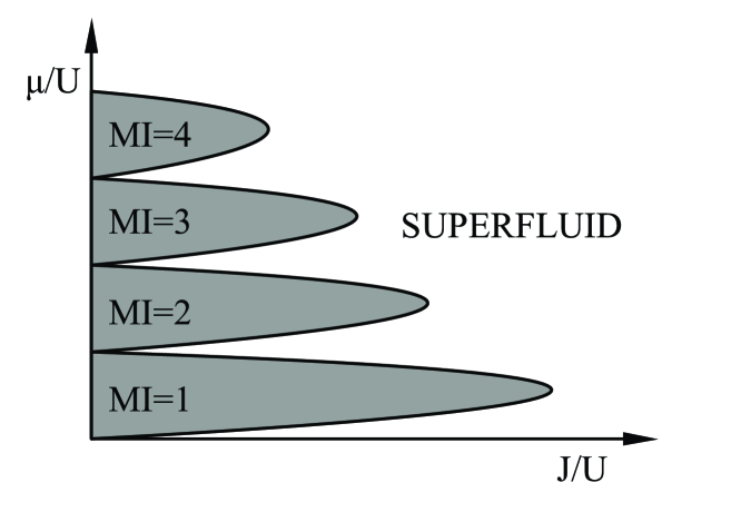
Figure 4.1: Phase diagram of the BH model. Inside the Mott insulator lobes the number of particles per site remains fixed.

$$\small{\hat{H}=\sum_{k=1}^{N}{\frac{U_{k}}{2}\hat{a}^{\dagger}_{k}\hat{a}_{k}(\hat{a}^{\dagger}_{k}\hat{a}_{k}-1)}-\sum_{k=1}^{N-1}{J_{k}(\hat{a}^{\dagger}_{k+1}\hat{a}_{k}+\hat{a}^{\dagger}_{k}\hat{a}_{k+1})}}+\sum_{k=1}^{N}\mu_{k}{\hat{a}_{k}^{\dagger}\hat{a}_{k}}.$$ (4.1)

As usual, the bosonic operators obey the commuting rules introduced before in equation (1.30), while $N$ is number of sites in the chain and the implicit integer $M$ is the number of bosons. The set of $U_{k}$ determine the intensity of the repulsion and the set of $J_{k}$ determine the intensity of the hopping across the chain. Finally, the set of $\mu_{k}$ account for the chemical potential. The BH model has been extensively studied since the discovery of superfluity in ${}^{4}He$ [4]. Although exact analytical solutions are not available, a lot of insight can be obtained out of careful inspection and clever mean field approaches. One important aspect of the study of the BH model is that such study is frequently carried out following a grand-canonical ensemble approach. This means it is assumed that the boson chain is being constantly fed by a powerful supplier that continuously provides bosons as well as energy in order to maintain the thermodynamic equilibrium. Nevertheless, it is important to mention that here we do not follow such description. Instead, our chain is fully isolated from any outside disturbance and the system state is given by the ground state of the Hamiltonian or by real-time unitary evolution. In figure 4.1 the phase diagram of the BH model interacting with a supplier bath is presented. As can be seen, the model is characterized by a superfluid phase and a Mott insulator phase. The difference between the phases is quite clear. In the superfluid state, bosons display non-vanishing hopping-scope-length. We can say that this phase is driven by hopping, since $J>>U$. On the other hand, in the Mott insulator state bosons remain tightly fixed on their hosting positions. In this phase hopping is highly hindered due to the loss of energy balance when the Mott insulator configuration is slightly disturbed, which results from $U>>J$. Formally, the Mott insulator phase is characterized by the following properties,

• Integer or commensurate density.

• Existence of an energy gap.

• Zero compressibility.

• Exponentially decaying correlations $\langle\hat{a}_{i}^{\dagger}\hat{a}_{j}\rangle$.

The first property is clear from the phase diagram of figure 4.1. The number of bosons per site is fixed inside the lobes that enclose the Mott phase. Commensurate densities correspond to configurations where the number of bosons is not an integer multiple of the number of sites, but a rational multiple. Over the y-axis and in between the lobes, the Hubbard model describes a superfluid, since the total number of particles fluctuates between two fixed values. The second property is of outstanding experimental importance, since the energy gap allows us to identify the Mott phase in the laboratory by spectroscopically probing the sample [5]. Additionally, the gap can be used in EIT experiments, where very long storage times have been observed [8]. The gap refers to the energy cost associated with making the bosons in the Mott state to jump out of their original positions. The third property means that the density of the system does not change as the chemical potential is varied, or equivalently, $\frac{\partial\rho}{\partial\mu}=0$. This also can be inferred from figure 4.1 by noticing that if we move from inside one of the Mott lobes in the direction of the vertical axis the number of particles would remain fixed as long as we stay in the Mott insulator state. We can think of this as a system in which the number of particles remains fixed despite the channels that define particle exchange between the system and its environment remain open.

Conversely, the superfluid is characterized by particle tunnelling all across the chain. The main properties of the superfluid are,

• Can exist at any filling.

• Eminently gapless.

• Finite compressibility.

• In one dimension, power law decay of correlations $\langle\hat{a}_{i}^{\dagger}\hat{a}_{j}\rangle$.

The first three properties stand opposite to the properties of the Mott insulator. The fourth property establishes that the superfluid is liable to develop correlations at long scale. This can be understood physically by noticing that as bosons jump from one place to the other, they distribute information all over the system. This property constitues the basis of the schemes that will be proposed in subsequent sections in this work. Both the Mott insulator state as well as the transition to a superfluid have been verified using cold atoms in optical lattices [6, 14, 7]. In a typical experiment, atoms are taken into a magnetic trap and then cooled down using an optical lattice of retroreflected diode lasers. This creates an arrangement of atoms where the resulting optical potential depths $V_{x,y,z}$ are proportional to the laser intensities and can be expressed in terms of the recoil energy,

$$E_{R}=\frac{\hbar k^{2}}{2m},$$ (4.2)

with $m$ the atomic mass and $k$ the wavelength number. To prepare 1D arrays, two lattice lasers are given high intensities in such a way that hopping can only efficiently take place across one axis [7]. In terms of experimental parameters, hopping and repulsion coefficients are given by,

$$J=A\left(\frac{V_{0}}{E_{R}}\right)^{B}e^{-C\sqrt{V_{0}/E_{R}}}E_{R},$$ (4.3)

and,

$$U=\frac{2a_{s}E_{R}}{d}\sqrt{\frac{2\pi V_{\perp}}{E_{R}}}\left(\frac{V_{0}}{E_{R}}\right)^{\frac{1}{4}},$$ (4.4)

where $V_{0}$ is the axial lattice depth, $V_{\perp}$ the depth of the lattice in the transverse directions, $a_{s}$ the $s$-wave scattering length, $d$ the lattice spacing. Capital letters represent experimental constants established by the geometry of the system. For example, for the experiment reported in reference [14] such constants are [74, 39],

$$A=1.397,\hskip 14.22636ptB=1.051,\hskip 14.22636ptC=2.121.$$ (4.5)

Spatial variations in $U$ and $J$ can also be implemented using detuned lasers sent through specific sections of the lattice as shown in reference [11].

Due to the vast number of quantum states necessary to span the Hilbert space, we must utilize MPS in order to be able to handle chain sizes of physical relevance. In an isolated boson chain, the conservation of the total number of bosons along with bosonic statistics determine the size of the basis needed to write an arbitrary state, namely,

$$\text{basis size}=\frac{(M+N-1)!}{M!(N-1)!}.$$ (4.6)

In practical terms, the amount of resources needed to simulate the system grows exponentially with the number of sites and bosons. Studies in boson chains using conventional bases have been done in chains of up to 10 sites and 10 bosons [75].

In order to find the ground state of the chain, we apply imaginary time evolution to a given initial state written in MPS. Such an initial state must have some overlap with the system ground state. The imaginary evolution is explicitly given by the formula,

$$|\psi_{G}\rangle=lim_{\tau\rightarrow\infty}\frac{e^{-\tau\hat{H}}|\psi_{0}\rangle}{||e^{-\tau\hat{H}}|\psi_{0}\rangle||}.$$ (4.7)

Additionally, we use second order Trotter expansion, which consists in splitting the evolution operator in a product of non-commuting operators as,

$$e^{-i\delta t\sum_{k=1}^{N}{\hat{A}_{k,k+1}}}=e^{-i\frac{\delta t}{2}\sum_{k=1}^{N/2}{A_{2k-1,2k}}}e^{-i\delta t\sum_{k=1}^{N/2-1}{A_{2k,2k+1}}}e^{-i\frac{\delta t}{2}\sum_{k=1}^{N/2}{A_{2k-1,2k}}}.$$ (4.8)

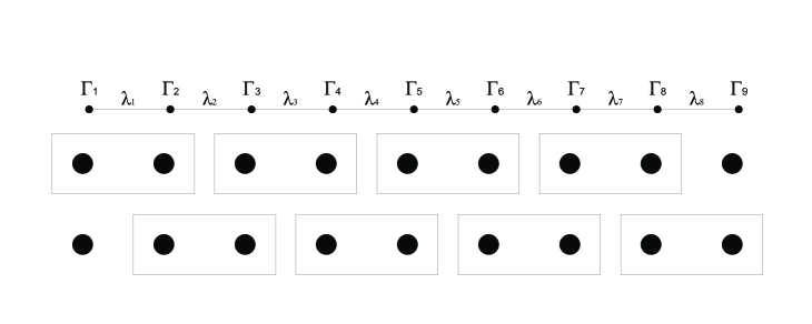
Figure 4.2: Sketch of operator splitting.

Each operator in the above product can be split in a product of several commuting operators, each corresponding to a specific pair of neighbour sites as shown in figure 4.2. After every updating step, in which the state is evolved using the Trotter formula, we retain all the Schmidt coefficients greater than $\lambda_{1}^{k}\times 10^{-14}$, where $\lambda_{1}^{k}$ is the greatest coefficient at site $k$. Then we use the Schmidt coefficients to find out the canonical representation. The maximum number of Schmidt coefficients in the chain is denoted by the letter $\chi$. The larger $\chi$ the more expensive it is for us to simulate the chain. In our program we use time slices in the range $10^{-5}<\delta\tau<10^{-3}$ depending on the chain size. Usually, simulations in long chains as well as very entangled chains require the smallest $\delta\tau$. Ground state convergence is evaluated through the criterion,

$$|1-\langle\psi(\tau)|\psi(\tau+\delta\tau))\rangle|<10^{-14}.$$ (4.9)

The accuracy of the final state depends on factors such as the length of the time slice, the original state, and the parameters in the Hamiltonian. In figure 4.4 we show simulations for trapped bosons in chains with different repulsion. The chosen regimes are compatible with experimental observations of Mott insulator (driven by repulsion) and superfluid (driven by hopping). The original state is a separable state for which the canonical decomposition can be easily written, namely, a state with one boson in each site. In this case the canonical decomposition can be written as,

$$\lambda_{1}^{[n]}=1,\forall n$$

$$\Gamma_{1,1}^{i[n]}=\delta_{i}^{1},\forall n.$$ (4.10)

For this state $\chi=1$. In a standard simulation, the maximum number of Schmidt coefficients $\chi$ gradually steps up as in figure 4.4. In most cases this variable saturates, but sometimes it instead peaks and dips, then reaches an equilibrium value. This is particularly the case for PTH chains with no repulsion. Figure 4.3 shows the behaviour of $\chi$ in imaginary time evolutions corresponding to different time slices. From such graph we can see that simulations with large $\delta\tau$ require large $\chi$. However, the number of steps necessary to reach convergence is fairly low. On the other hand, when the size of $\delta\tau$ is reduced, the maximum $\chi$ goes down while the number of steps necessary to converge the state goes up. We can actually establish the appropriate value of $\chi$ by comparing the energy of the obtained ground state with the exact analytical results. We know that the energy of a PTH chain with $M$ bosons is given by,

$$E_{G}=-\lambda\left(\frac{N-1}{2}\right)M.$$ (4.11)

Similarly, we can estimate the energy $E_{G}$ of the state written in tensor notation from the change in the state norm assuming that the state itself is not hugely different from the ground state,

$$e^{-\delta\tau\hat{H}}|\psi_{G}\rangle=e^{-\delta\tau E_{G}}|\psi_{G}\rangle.$$ (4.12)

Table 4.1 shows the energy values obtained in this way. We can see that states obtained using relatively big $\delta\tau$ slightly underestimate the ground energy. In this case we can say that the theoretical error involved in decomposing the evolution operator in a product of small unitary transformations is more influential than roundoff errors. Additionally, we can see there is an optimal value of $\delta\tau$ for which the ground state energy contains the maximum number of significant correct figures without it going below the actual ground energy. Similar analyses in chains of different sizes show that in PTH chains optimal convergence is achieved using $\delta\tau=\frac{10^{-3}}{N}$. In the general case, the optimal size of $\delta\tau$ is inversely proportional to the scope of the boson tunnelling in the ground state, which depends on the intensity of the hopping. Hence, for arbitrary hopping and repulsion profiles we can write,

$$\delta\tau=\frac{10^{-3}}{N_{e}},$$ (4.13)

where $N_{e}$ is the effective tunnelling length of bosons in the state, which must be estimated out of physical insight.

Figure 4.3: Ground state convergence in PTH-repulsionless chains for 10 sites and 10 bosons. These simulations correspond to the energy values in table 4.1.

Figure 4.4: Simulations in boson chains of 100 sites and 100 bosons using TEBD. The error bars in the lower graphs represent fluctuations. Left: $U_{k}=2$, $J_{k}=0.14$, $\mu_{k}=0.0046(k-50)^{2}$ and $\delta\tau=0.00001$. Right: $U_{k}=0.42$, $J_{k}=0.14$, $\mu_{k}=0.0046(k-50)^{2}$ and $\delta\tau=0.00005$. All these constants are given in arbitrary units.

$\delta\tau$	$E_{G}$
0.1	-.902854035422649E+02
0.05	-.900740540911757E+02
0.01	-.900029984667920E+02
0.005	-.900007499039339E+02
0.001	-.900000299962281E+02
0.0005	-.900000074855496E+02
0.0001	-.899999999159858E+02
0.00005	-.899999988644993E+02

Table 4.1: Ground state energy in PTH-repulsionless chains with no repulsion for 10 sites and 10 bosons. These values correspond to the energy graphs in figure 4.3. The value closest to $90$, the actual energy, is written in boldface.

As it has been pointed out in several studies [76, 63], it is the variable $\chi$ that ultimately determines the simulation efficiency. This fact is quite reasonable, on the one hand $\chi$ defines how much memory is necessary to store the canonical decomposition, and on the other hand it determines the number of numerical operations that must be performed in order to upgrade the state [22, 63]. Similarly, this number is directly linked to the entanglement profile displayed by the state. As can be seen in figure 4.4, states showing more entanglement also develop higher $\chi$. Therefore, practical simulations can be done in systems where analytical correlations are not too strong. In the BH model particularly, we know that close to the Mott insulator regime quantum correlations are quite moderate. Additionally, the superfluid state is characterized by certain regularity which somehow keeps $\chi$ from growing indefinitely. However, it is the state in between the phases what brings more challenge. In this case, a kind of strongly enhanced entanglement embraces the state and $\chi$ grows well above manageable limits. According to mean field theory, the transition from Mott insulator to superfluid in the thermodynamic limit takes place at $\frac{U}{J}=11.6$ [4, 5] for a chain with unit filling. Figure 4.4 shows simulations on each side of such transition point. These graphs show the characteristics of the Mott insulator and the superfluid. As can be seen, the expectation value of the number of particles in the Mott state shows integer density over a wide range of positions as well as small fluctuations. The superfluid features large fluctuations, which anticipates the existence of long range correlations. In general, the simulations of the superfluid require more computational resources than the Mott state. As discussed before, the Mott state is characterized by the existence of a gap as well as integer density. The superfluid on the other hand is associated with intense boson hopping and long range correlations.

Figure 4.5: Dynamics of a boson chain using TEBD. The system is prepared in a Mott insulator state with one boson per site. The chain parameters are characteristic of the superfluid phase, namely, $U_{k}=0.4E_{R}$, $J_{k}=E_{R}$ and $\mu_{k}=0$. In order to get reliable results, we use a very thin time slice $\delta t=0.00005E_{R}/\hbar$. As a way of keeping the size of the canonical decomposition at a manageable level, we deliberately fix $\chi_{MAX}=50$. It has been verified that the same simulations with $\chi_{MAX}=60$ generate identical results.

Similarly to ground state simulations, the performance of TEBD in the real time context is highly dependent on the variable $\chi$. However, the development of this variable in dynamical problems is different from the one observed in imaginary-time evolution. While for the latter case $\chi$ saturates to a reasonable value, for the real time case it grows steady, the same that the number of resources necessary to describe the state [77]. As a consequence, numerical dynamics using TEBD is usually restricted to short times regimes, where the size of the canonical decomposition can still be handled. Alternatively, we can set a maximum value for $\chi$. This allows us to obtain results for extended time intervals in the range where the system behaviour remains consistent. Figure 4.5 presents several dynamical quantities obtained from simulating a boson chain prepared in a Mott insulator state with one boson per site. The apparent lack of dynamics in the graph of the expectation value of the number of bosons can be explained by noticing that in a regularly filled chain with one particle in every site the boson hopping generates equitable mass exchange, specially around the central part. Therefore, the expectation value remains relatively stable through very long times. However, the system develops an underlying dynamics, as can be inferred from the graph of fluctuations, given by the formula,

$$f_{i}=\sqrt{\left\langle\hat{n}_{i}^{2}\right\rangle-\langle\hat{n}_{i}\rangle^{2}},$$ (4.14)

where $\hat{n}_{i}=\hat{a}_{i}^{\dagger}\hat{a}_{i}$. As can be seen, fluctuations saturate faster than the von Neumann entropy between complementary blocks. This suggests that the incidence of high order effects in the chain is very important, not least in the short run. It also can be seen that the system dynamics close to the chain ends is notoriously different from the flat patterns displayed over the central part. These border effects are characteristic of chains with open boundary conditions [78]. In the long run we expect that these border fluctuations propagate all across the chain and the system acquires a wavy profile. Nevertheless, long time simulations are likely to contain flawed data as a result of the truncation of MPS.

In this section we have given a short review of the BH model, emphasising in the aspects that are more relevant to our investigation. We have described the use of imaginary-time TEBD in boson chains and its relation with the phases associated with the model. Similarly, we have discussed the main characteristics of real-time numerics and the way our simulations are affected by them. In chains with strong correlations, which are the focus of subsequent sections, the presence of entanglement considerably hinders the simulation efficiency. As a result, we can estimate the ground state as well as the dynamics of highly entangled chains in systems of moderate size. Further analysis and complementary results are to be presented in subsequent sections.

Chapter 5 Entanglement and its relation with physical processes in engineered Bose-Hubbard chains

As the increasing development of cooling techniques in optical lattices has led to the experimental implementation of engineered quantum systems, it has become important to explore how the quantum nature of such configurations can be used in quantum computation processing and other interesting fields of research. Consequently, given the connection between entanglement and quantum computation, we have concentrated on studying the entanglement in systems that are now the object of intensive experimental exploration. In doing so we have focused on one kind of entanglement that, to our understanding, is most useful for developing quantum computation tasks, this is, the entanglement between distant places of the chain. Likewise, given the volume of technical complexities associated with a multi-disciplinary investigation, we have narrowed this research to the study of entanglement between the ends of the chain and the entanglement register provided by the coefficients of the canonical decomposition. In addition to the characterization of entanglement, in this section we look at the relation of such entanglement with the physical mechanisms associated with the model under scrutiny.

5.1 End-to-end entanglement and generalities

Figure 5.1: Potential realization of BH model with spatially dependent repulsion in an optical lattice.

In a boson chain with no chemical potential or constant chemical potential on each site, the Hamiltonian is given by,

$$\small{\hat{H}=\sum_{k=1}^{N}{\frac{U_{k}}{2}\hat{a}^{\dagger}_{k}\hat{a}_{k}(\hat{a}^{\dagger}_{k}\hat{a}_{k}-1)}-\sum_{k=1}^{N-1}{J_{k}(\hat{a}^{\dagger}_{k+1}\hat{a}_{k}+\hat{a}^{\dagger}_{k}\hat{a}_{k+1})}}.$$ (5.1)

The reason for not including additional terms is because this slightly simplified form allows us to focus exclusively on repulsion and hopping, so that the effects of chemical potential can be considered on the light of the results obtained in this simpler scenario.

Figure 5.2: Left. Particle distribution profile and fluctuations for the ground state in PTH chains. (—) No repulsion at all. ($--$) $U_{2-7}$ = 100. Right. Ground state entanglement between the ends of a chain of eight places and eight bosons against repulsion. PTH and repulsionless ends are assumed . Fitting $y=0.91-0.34e^{-0.035x}$.

From our initial simulations we observe that ground state entanglement between the ends is highly sensitive to the particle distribution profile along the chain. This is due to the effect of tracing out intermediate sites in order to get the reduced density matrix of the terminals. When population is accumulated in the middle of the chain we must trace out states with a considerable number of particles in order to obtain the mixed state of two distant sites at the borders. Lower population at the ends implies a lower number of possibilities for distinct particle number states available at the ends and consequently a lower ability to correlate particle numbers between these sites and entangle them. Thus for the repulsionless case and PTH, where population accumulates primarily in the middle of the chain (which is shown in figure 5.2), the entanglement is vanishingly small. The choice of PTH, as opposed to a uniform $J_{k}$, thus clearly illustrates the negative effect of population concentration in the middle of the chain. To get a higher entanglement, we then proceed to deliberately frustrate boson accumulation in the central part of the chain by evenly increasing the repulsion in every site but the ends which in turn are left repulsionless (figure 5.1). This approach allows us to look closely at the physical mechanisms underlying the interplay between hopping and repulsion and its effects on quantum correlations at long distances. In figure 5.2 we can see how the boson population in intermediate positions concentrate on the lowest levels of occupation creating a fine arrangement of superfluid particles that connects the ends, which in turn become highly populated. Figure 5.2 also depicts the behaviour of Log-negativity as a function of repulsion. It can be seen that entanglement grows monotonically, undergoing saturation for large repulsion, suggesting that maximum entanglement is achieved when particles in intermediate places behave as hardcore bosons. In this limit, bosons find it difficult to stay at the intermediate positions as the hopping of particles from neighbour sites would give rise to multi-occupied states with strong repulsion. Instead, bosons organize in superposition states that on average contain only half a boson per site for the intermediate sites, creating a globally delocalized profile that favours long-range quantum correlations. Similarly, analogous plots corresponding to expectation values of number of particles also display saturation for high repulsion, establishing a clear signature of rescaling behaviour, that is, bosons reorganize under the influence of larger repulsion constants in such a way that the phenomenology of the system is altered, roughly, just by a proportionality factor. Similar conclusions can be drawn for chains with constant coefficients $J_{k}$ and repulsionless ends, although PTH chains are more efficient at enhancing entanglement. For instance, in a chain of ten sites, ten bosons, PTH and high intermediate repulsion $U_{2-9}=100$, Log-negativity was found to be $0.83$ against $0.60$ of the same chain with uniform unity hopping. In the study ahead, we further explore this remarkable behaviour.

5.2 Entanglement in the ground state

Figure 5.3: Numerical cost of ground state simulations of Hamiltonian (5.1) for $N=M=20$. These computations correspond to some of the points in figures 5.5 and 5.6. Left. CH. Right. PTH.

The analysis in the previous section suggest that the relative population at the ends is in some manner linked to EEE. Indeed, after some test computations we found that as a consequence of the universality characteristics of the problem it is appropriate to plot our results using the fraction of particles on the ends (dimensionless),

$$\zeta=\frac{\langle\hat{a}^{\dagger}_{1}\hat{a}_{1}\rangle+\langle\hat{a}^{\dagger}_{N}\hat{a}_{N}\rangle}{M},$$ (5.2)

which allows a comparative perspective of the system behaviour for different scales. $\zeta$ varies according to the intensity of the repulsion in intermediate sites. As can be seen in figure 5.2-left, when repulsion is small few particles remain on the ends and $\zeta\approx 0$. From the same graph it follows that when repulsion is strong the amount of particles on the ends is maximum and,

$$\zeta=\frac{1}{2}+\frac{1}{M}.$$ (5.3)

Notice that $\zeta$ keeps a close relation with the repulsion constant $U_{k}$. This variable $\zeta$ enables us to depict our results for different chain sizes in a comparative manner. Before presenting our results and the corresponding analysis, we want to briefly comment on the computational cost associated with the simulations shown on this section. In order to make our analysis as robust as possible, we performed computations in chains as large as our resources allowed them to be. In a strongly entangled chain, nevertheless, TEBD is not very efficient, and the biggest system we worked on corresponds to $20$ bosons in $20$ sites. These computations, however, are considerably demanding (using normal desktop computers, finding the ground state can take up to two weeks). As a comparison, note that the maximum $\chi$ in the simulations presented in figure 4.4 for systems of $100$ bosons in $100$ places is always below $60$ while the same cost-measuring parameter goes well above $140$ in figure 5.3 which corresponds to the results to be shown in this section.

Figure 5.4: Entanglement between the terminals and the rest of the system in a boson chain governed by Hamiltonian (5.1) and with no repulsion on the ends. Left. CH. Right. PTH. As usual, the number of boson in each chain is equal to the indicated number of sites.

In our physical model, independently of the particularities of the hopping profile, the ground state of repulsionless chains is eminently superfluid, although with most of the tunnelling taking place in the central part, leaving the terminal positions nearly empty (figure 5.2-left). In this case entanglement is at the same time strong and localized. Indeed, in these circumstances entanglement between half-chain-blocks is strongly enhanced. Similarly, particles are forced to tunnel through longer distances and correlations develop at longer scales as repulsion in intermediate positions climbs up. Additionally, bosons increasingly migrate towards the terminal positions since the repulsion prevent particles from staying in intermediate sites. Outstandingly, on account of the repulsionless ends, boson fluidity stands no matter how strong the repulsion in intermediate sites is. As repulsion slowly grows away from zero, entanglement between the chain halves goes down while entanglement between the ends and the rest of the system goes up, an indication that the originally localized correlations are being spread all over the chain following the particle distribution profile. When repulsion is increased even more, the terminals start getting macroscopically occupied so that the expectation value of the number of bosons and the fluctuations in intermediate sites both go down asymptotically towards $\frac{1}{2}$, which indicates that bosons get highly delocalized. In this case correlations among places near the ends and in opposite sides of the chain are strongly enhanced, in contrast to the correlations in the centre of the chain. This can be seen in the graphs of figure 5.4 where, interestingly, von Neumann entropy between both ends and the rest of the system slightly comes down after the original redistribution of entanglement mentioned above occurs. This effect is more evident for the CH case. The decrease in the entanglement between the ends and the rest of the system can be interpreted as a reduction of the correlations in intermediate sites which takes away local combination of states with substantial entangling potential. On the other hand, this reduction of the correlations between both ends and its complement is convenient for the emergence of EEE, since the reduced state of the terminals becomes closer to a pure state. This fact alone, however, is not sufficient for the arising of EEE. Even if the state of the terminals is completely pure, it is possible that the quantum state of such reduced system is separable. In this context it is interesting to explore the mechanisms that ultimately define the onset of long-range entanglement.

The issues discussed so far are independent of either hopping profile we feed into Hamiltonian (5.1). We now want to focus on those characteristics associated exclusively with the values given to the hopping coefficients. Figure 5.5 summarizes the results we obtained from computing the logarithmic negativity in both CH and PTH chains. Notice that the curves in figure 5.5 are analogous to the results in figure 5.2 which are depicted in a slightly different way.

Figure 5.5: Logarithmic negativity of the terminals. In all cases the number of bosons in the chains is equal to the indicated number of sites.

As a matter of fact, EEE has a more interesting behaviour in PTH chains than in CH chains. The most notorious advantage of PTH is the persistence of entanglement, even when the number of sites and bosons augment. In contrast, the amount of entanglement in CH chains does not stand against increasing chain size. Similarly, when the entanglement values are seen at any given fixed $\zeta$, it is clear that PTH chains display more EEE than their CH equivalent. This is straightforward since in figure 5.5 PTH entanglement arises well before CH entanglement. Given the increasing cost of the simulations, specially for the PTH case, not all the possible values of $\zeta$ are considered, but further information can be extrapolated from the data at hand. Indeed, PTH curves fit nicely into a single line with slope $1.75$. As expected, the cost of the simulation is proportional to the amount of entanglement, but we can get a reliable scaling characterization from the information contained in figure 5.5. Correspondingly, numerical fitting yields

$$EEE^{PTH}_{\zeta=0.5}\sim log(N^{0.1}),\text{and}$$

$$EEE^{CH}_{\zeta=0.5}\sim log(N^{-0.2}).$$ (5.4)

Indeed, the logarithmic behaviour of EEE has been inherited from the measure we use to quantify EEE, but the fitting formally establishes that the PTH profile provides a platform that is highly convenient to entanglement.

The fact that entanglement is better for some configuration of parameters than for others makes us wonder what is so special about a hopping profile that delivers substantial entanglement between the terminals. Curiously, the particle distribution profile in general looks like the one in figure 5.2-left for chains with very high repulsion in intermediate sites, no matter which hopping profile, PTH or CH, we choose. This means that the mechanisms giving rise to entanglement must be determined by high order terms of the imaginary-time-evolution operator [16]. Such high order terms induce essentially two kinds of physical processes, namely,

• Exchange of more than one particle among places of the chain.

• Exchange of particles among distant places of the chain.

Figure 5.6: Entanglement between the halves of the chain. In all the graphs the number of bosons in equal to the indicated number of sites. Top. CH. Bottom. PTH.

These mechanisms can take place simultaneously, and as a result, correlations develop at a macroscopic scale. When the conditions are optimal, as for instance with PTH, correlations are massively enhanced and this leads to long range entanglement. This interpretation coincides with further results, especially with the logarithmic negativity graphs shown in figure 5.6. As can be seen, entanglement between the halves of the chain decreases monotonically as the repulsion in intermediate sites is turned up. Such behaviour is in certain way not surprising since as repulsion becomes more intense, more particles are forced away from the centre and into the terminals, which reduces the amount of “quantum channels” that can be used by every half-chain block to speak directly to each other. Nevertheless, the behaviour of logarithmic negativity in PTH chains is quite different. In such a case the graphs display a clear minimum instead of a constantly falling curve. Consequently, in spite of the reduction in communication resources, there is a critical repulsion value for which entanglement stops falling and slowly turns its way up. The bigger $N$, the sharper the effect, which suggests this would lead to a second order phase transition in the thermodynamic limit. This sudden reinforcement of entanglement can be understood as coming from an enhancement in the particle exchange between the chain terminals. Certainly, when the delocalization length of bosons is equal to the distance between the chain ends, particles held on the terminals can be exchanged directly between the ends. This induces a transition of the system state, since those particles originally squeezed against the chain borders are suddenly unleashed and, instead of being highly localized around the system boundaries, their wave functions now envelop the chain to its whole extent, keeping on average most of the wave function weight on the terminals. This interesting effect can also be intuitively identified by assuming a particle-like behaviour of bosons. Indeed, we can think that as repulsion in the middle is continuously turned on, bosons are obliged to hop through longer distances and thereby become more and more delocalized. The enhancement of entanglement is therefore determined by the tunnelling scope rather than by plain particle accumulation, although the latter is a necessary condition for EEE emergence. In CH chains, the form of von Neumann entropy between both halves in consistent with a regime in which entanglement is being continuously redistributed across the system as a result of increasing tunnelling scope, but the fact that there is no turning point in figure 5.6-top indicates that such hopping never takes place across the complete length of the chain. However, such hopping is enough to induce EEE at finite $N$, but not in the thermodynamic limit since EEE dies down against increasing chain size. It is as if such finite $N$ entanglement results from the overlapping of neighbouring wave functions. The transition to a strongly entangled state takes place when such local wave functions flatten and successively combine to create a strongly global description of the state. Once the previously mentioned long scale tunnelling takes over, increasing the repulsion in intermediate sites reinforces end-to-end exchange and induces an increase in the amount of entanglement shared by the terminals, as can be seen in figure 5.6-bottom. This can also be understood in terms of the so called healing length, which defines the distance that takes the condensate to form its bulk. We can say that the healing length determines the space over which the superfluidity of the system is suppressed. In terms of physical constants, this length scales as $L_{healing}\sim\frac{1}{\sqrt{U}}$. In ${}^{4}He$, the healing length is around $0.1nm$. The phenomenon that we report in this section can be seen as a suppression of the healing length, in such a way that superfluid features are present all over the chain, and then these features are reinforced by the PTH hopping profile.

5.3 Entanglement and dynamics

Figure 5.7: Logarithmic negativity for $N=M=8$ and CH. The system is prepared in a Mott insulator state with one boson in each site. As can be seen, strong repulsion constants in intermediate places are necessary to induce substantial EEE.

Here we study how entanglement arises dynamically in boson chains with superfluid characteristics. This is the most relevant situation since any form of entanglement is null in the Mott insulator state. In the discussion that follows we assume that our chains are initially prepared in a Mott insulator state and the parameters are suddenly changed to generate the dynamics. The new set of parameters correspond to a given hopping profile, CH or PTH, and a given repulsion profile which always maintains the ends repulsionless. This is the most natural scenario one can expect in a BH chain where one first prepares the Mott state with one boson per site and then turns all the interactions globally, the same as in [48, 79, 80], but opposite to the approach in [81, 78] where the quench goes from the superfluid to the Mott insulator. As a generic example we present in figure 5.7 the evolution of the logarithmic negativity for different values of intermediate repulsion. In a chain with all the repulsion constants set to zero, EEE shows very little development in the course of evolution as can be seen in the indicated figure. Dynamics in repulsionless chains is, in fact, known to lead to a progressive thermalization of reduced density matrices of each site [79, 80]. Two site entanglement is thus very low in this repulsionless scenario. High repulsive evolution, on the other hand, shows a less regular profile, product of interference among many unsynchronized phases accumulated locally. From figure 5.7 we infer that as in the case of ground state entanglement, dynamic entanglement does not build up unless a significant accumulation of particles assists the enhancement of fluctuations at the ends. As can be observed in the evolution patterns of chains with high repulsion in intermediate sites, the amount of entanglement contained in the system after reasonable times can be significant, yet smaller than what can be obtained from the ground state in optimal configurations (compare with figure 5.2-right). Here, we assume uniform hopping but our conclusions are valid also for PTH.

Figure 5.8: Particle distribution in bosonic chains for $N=M=20$. The system is prepared in a Mott insulator state with one boson per site. Strong repulsion constants in intermediate sites forces the bosons into the ends. Left. CH and $U_{2-19}=100E_{R}$. Right. PTH and $U_{2-19}=200E_{R}$.

In order to identify relevant differences between the entanglement behaviour in chains with different hopping profiles, we found it necessary to perform simulations in chains of up to $20$ places with $20$ bosons. As we already know that strong repulsion is necessary to induce EEE, we just set high repulsion constants on every site except the terminals and simulate the evolution using the TEBD algorithm. The resulting dynamics can be seen in figure 5.8, where the expectation value of the number of particles is plotted as a function of time. The ends get macroscopically occupied and tunnelling in intermediate places intensifies. EEE arises some time after the ends have been occupied, as can be appreciated in the graphs of figure 5.9. In general, the bigger the chain the longer it takes for EEE to emerge. For PTH, a natural time scale is determined by the transmission period, $T=\pi$, on account of our particular choice of $\lambda=2$. Entanglement shows up more or less at half of the period, $t\approx\frac{\pi}{2}$, when some particles have travelled from one end of the chain to the other. It could be, however, that EEE in longer chains behave differently, since repulsion in intermediate places hinders the boson mobility. This negative effect is likely to be more pronounced when transport takes place at long distances. For longer times entanglement might grow above the values reported in figure 5.8, independently of the hopping profile, but this effect is hard to follow as long time simulations require additional computational resources [77, 76].

Figure 5.9: The system is prepared in a Mott insulator state with one boson in each site. These graphs correspond to equivalent systems shown in figure 5.8. Left. CH and $U_{2-19}=100E_{R}$. Right. PTH and $U_{2-19}=200E_{R}$.

5.4 Entanglement and perturbative dynamics

We have seen how boson chains can be made to contain substantial entanglement in the ground state as well as in the course of dynamics. Ideally, if both approaches are combined we then could multiply the amount of entanglement in the chain, which would result in a highly beneficial use of the several quantum degrees of freedom that come from the multiple possibilities of arranging a given number of particles on the system. Hence, we now assume that a chain initially prepared in an entangled ground state evolves by the action of a perturbation added to the original Hamiltonian. The reason for choosing a perturbation rather than an abrupt change of parameters in the Hamiltonian is because a perturbation is expected not to modify the particle distribution profile substantially, so that the terminals of the chain remain macroscopically populated which has been already identified as a necessary condition for entanglement generation. In formal terms, the state evolution is given by,

$$|\psi(t)\rangle=e^{-it\hat{H}_{1}}|\psi_{g}\rangle,$$ (5.5)

where,

$$\hat{H}_{1}=\hat{H}_{0}+\epsilon\sum_{j=1}^{N}\hat{h}_{j},$$ (5.6)

in such a way that $|\psi_{g}\rangle$ is the ground state of Hamiltonian $\hat{H}_{0}$, from equation (5.1), and $\epsilon$ is a small real number which determines the intensity of the perturbation. $\hat{h}_{j}$ represents a local operator acting on site $j$. The explicit form of operators $\hat{h}_{j}$ is to be worked out according to our convenience. For consistency, the first condition to be satisfied is,

$$[\hat{H}_{0},\sum_{j=1}^{N}\hat{h}_{j}]\neq 0,$$ (5.7)

otherwise dynamics would be trivial. In order to simplify our analysis we assume that the local operators can be written as functions of the corresponding local number operator,

$$\hat{h}_{j}=h_{j}(\hat{n}_{j})$$ (5.8)

where,

$$\hat{n}_{j}=\hat{a}_{j}^{\dagger}\hat{a}_{j},$$ (5.9)

so that we can now focus on the functional forms $h_{j}(x)$ rather than in quantum operators. We can establish a non-vanishing commutator between the perturbation and the Hamiltonian by defining,

$$h_{j}(x)=kx,$$ (5.10)

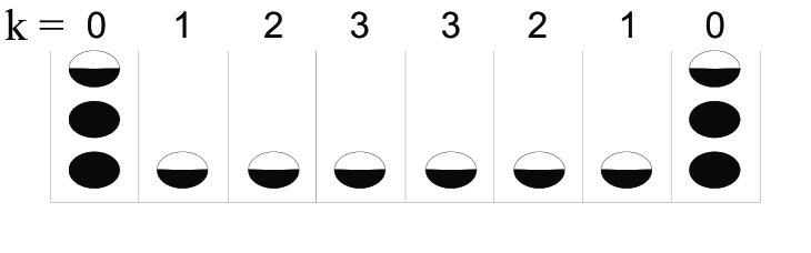
Figure 5.10: Sketch of bosons spread across a chain of repulsionless ends.

where $k$ is the integer distance between site $j$ and the closest end, as indicated in figure 5.10. This form holds only for intermediate places. Similarly, to determine the form of the operators on the terminals, $h_{1,N}$, the primary factor to take into account is the optimization of boson-transfer from intermediate sites towards the ends. If the expectation value of the number of particles remains stable during time evolution we can carry out a classical analysis in the basis of the number of bosons. Let us think that in the configuration shown in figure 5.10, which sketches one of the particle distribution shown in figure 5.2-left, we take half a boson from the centre of the chain and put it in the closest terminal. We can assume that this repositioning does not cause much change in the average value of $\hat{H}_{0}$, since there is no contribution from the repulsion terms for bosons in intermediate positions, because repulsion is zero for one or zero bosons, or for bosons on the chain ends, because repulsion is off on the terminals. As a consequence, we would expect that the change in the average values of the system could be calculated focusing only on the averages of the perturbative potential. Additionally, because we want particles to go from the middle of the chain to the terminals and vice versa, we need that the energy cost of extracting particles from intermediate positions balances the energy cost of putting the same particles on the chain ends. For example, starting from the state depicted in figure 5.10, if all the particles go consecutively from the middle of the chain to the ends, the first process to take place is that bosons in positions with $k=3$ disappear from their respective positions and pop up on the terminals. The corresponding energy balance can be written as,

$$h\left(n_{0}+\frac{1}{2}\right)-h(n_{0})=\frac{3\epsilon}{2}.$$ (5.11)

In this expression $n_{0}$ represents the expectation value of the number of particles on one of the terminals, which can be simply taken as $n_{0}=2.5$ for this specific case. Once this process is over, there are fewer particles in intermediate sites and more on the ends. Hence, taking first bosons with $k=2$ and putting them on the ends and then doing the same for bosons with $k=1$ we obtain,

$$h\left(n_{0}+1\right)-h\left(n_{0}+\frac{1}{2}\right)=\epsilon,$$

$$h\left(n_{0}+\frac{3}{2}\right)-h\left(n_{0}+1\right)=\frac{\epsilon}{2}.$$ (5.12)

In a chain of size $N$ these equations lead to one single expression, namely,

$$h\left(n_{0}+\frac{1}{2}\left(\frac{N}{2}-k\right)+\frac{1}{2}\right)-h\left(n_{0}+\frac{1}{2}\left(\frac{N}{2}-k\right)\right)=\frac{\epsilon k}{2}.$$ (5.13)

After some preliminary tests we find that the optimal choice for the unknown function is,

$$h(x)=c_{2}x^{2}+c_{1}x.$$ (5.14)

Constants $c_{2}$ and $c_{1}$ are used to balance equation (5.13). Combining these equations and after some simplification we get,

$$c_{2}\left(n_{0}+\frac{1}{2}\left(\frac{N}{2}-k\right)\right)+\frac{c_{2}}{4}+\frac{c_{1}}{2}=\frac{\epsilon k}{2}$$

$$\Rightarrow c_{2}n_{0}+\frac{c_{2}N}{4}+\frac{c_{2}}{4}+\frac{c_{1}}{2}\mbox{\boldmath$-\frac{c_{2}k}{2}$}=\mbox{\boldmath$\frac{\epsilon k}{2}$ }$$ (5.15)

In order to work out a set of constants valid for every $k$ we must define,

$$c_{2}=-\epsilon,$$

$$c_{1}=\left(\frac{N+1}{2}+2n_{0}\right)\epsilon.$$ (5.16)

Figure 5.11: Evolution in chains of $N=M=8$ for PTH and $U_{2-7}=100E_{R}$. The system responds according to the intensity of the perturbation. Equivalent graphs corresponding to population averages deviate less than 2% from their initial values. Left. Fluctuations in the number of bosons allocated in one end of a chain. Right. Dynamical entanglement.

Moreover, for a perturbation written as above, the mean number of bosons does not fluctuate much since the dynamics is still governed by a Hamiltonian with strong repulsion coefficients in intermediate sites and bosons are forced to stay on the ends. In this situation one would expect that the evolution is dominated by high order dynamics such as the exchange of particles between the terminals and the rest of the system. Evidence of this can be seen in the graph of fluctuations shown in figure 5.11-left. As can be expected from our particular choice of function $h(x)$, the transit of bosons between the ends and the rest of the chain is enhanced and therefore the fluctuations on the terminals are developed according to the strength of the perturbation. Certainly, such enhancement of fluctuations leads to an improvement of communication between distant places which results in entanglement. Figure 5.11-right shows Log-negativity as a function of time for different perturbation intensities. Roundoff errors accumulated in the ground state during the imaginary time evolution cause slow oscillations in the dynamics at $\epsilon=0$, but these are tiny compared with the more complex evolution seen at finite $\epsilon$. In the initial stages of evolution the dynamics is characterized by a sharp increase of quantum fluctuations on the ends of the chain accompanied by little change in the expectation value of the number of bosons. Hence, entanglement development is enhanced while avoiding massive migration of bosons towards the centre of the chain. This effect is maximal at around $\epsilon=0.1$ and becomes less important for higher values of $\epsilon$, where perturbative terms induce a less predictable dynamics. Significantly, entanglement generation is improved not by adding interaction terms to the Hamiltonian but by evolving an already entangled state using a locally-tuned perturbative potential.

Figure 5.12: Logarithmic negativity in chains of $N=M=14$ for both CH and PTH. PTH lines are thicker than their CH equivalents. EEE in the ground state can be improved as a result of dynamics in PTH chains. $\chi=200$ for PTH and $\chi=100$ for CH.

In order to see if this effect lingers on when the size of the chain is increased, we applied the same ideas to chains of $N=M=14$. Interestingly, EEE behaves in a very similar way than in the previous case, with almost the same values at the same times, as indicated in figure 5.12. In this figure we also include CH results, which make it clear that the enhancement effect is characteristic of PTH chains. This is a curious matter, since the perturbative analysis does not include any reference to any specific hopping profile, it just balances the energy costs coming from different terms in an optimal trajectory. In principle, one can think that the lack of entanglement development may be due to either,

• Lack of boson mobility.

• Dynamics with deficient entangling capability.

In general, entanglement seems not to team up with CH, as opposite to PTH. Whatever the specific reason why this compatibility between entanglement and some specific profiles occurs, our results clearly suggest that particle transport plays a crucial role in the development of correlations in the quantum state.

5.5 Entanglement detection

Figure 5.13: Entanglement detection

In this short section, we want to explore how this entanglement could be measured in the laboratory. Once bosons are cooled down in the ground state or after evolution has taken place and the interactions are turned off, the detection protocol studied in [82, 83] could be used. The idea behind most entanglement-verification procedures is to uncover the non-local behaviour of the entangled state. This non-locality can manifest itself in a spatial basis, such as it happens, for instance, while probing the non-locality of a single particle [56], but it can also arise in the basis of the number of particles. The protocol proposed in [82] exploits the idea presented in [83], that there cannot be a pure separable state with fixed particle number and full interference among spatial modes. Let us suppose that after the intermediate degrees of freedom in the chain has been reduced, we are left with a density matrix $\hat{\rho}$, which represents our knowledge of the resulting two-side mixed state, or equivalently, the state of the chain ends. Following the protocol of reference [82], bosons on the terminals are sent through a 50:50 splitter and then the number of particles on the outputs is measured, for example following the technique proposed in [15].

The effect of the 50:50 splitter is to combine the modes of the original system, $\hat{a}_{1}^{\dagger}$ and $\hat{a}_{N}^{\dagger}$, according to the following transformation,

$$\hat{a}_{1}^{\dagger}=\frac{1}{\sqrt{2}}(\hat{a}_{c}^{\dagger}+\hat{a}_{d}^{\dagger}),$$

$$\hat{a}_{N}^{\dagger}=\frac{1}{\sqrt{2}}(\hat{a}_{c}^{\dagger}-\hat{a}_{d}^{\dagger}),$$ (5.17)

where $\hat{a}_{c}^{\dagger}$ and $\hat{a}_{d}^{\dagger}$ are the modes of the system after the 50:50 splitter. Such splitter can be considered as the physical place where interference between the bosonic bulks takes place. In this way, as $\hat{a}_{c}^{\dagger}$ and $\hat{a}_{c}$ are the operators describing the particle occupation on one of the outputs, EEE can then be detected from the experimentally measurable variable,

$$\epsilon_{AB}=tr(\hat{a}^{\dagger}_{c}\hat{a}_{c}\hat{\rho})-\frac{N}{2}=tr(\hat{a}^{\dagger}_{1}\hat{a}_{N}\hat{\rho}),$$ (5.18)

where,

$$tr(\hat{a}^{\dagger}_{c}\hat{a}_{c}\hat{\rho}),$$ (5.19)

is the number of particles in one output and $\hat{\rho}$ is the reduced density matrix of the ends. As it is characteristic of a good entanglement measure,

$$\epsilon_{AB}=0,$$ (5.20)

for separable states and,

$$\epsilon_{AB}>0,$$ (5.21)

for entangled states. In this way, entanglement can be detected by just comparing the amount of bosons in one output, which can be done with relative efficiency. In order to show how this method can be applied to our model, we present in figure 5.13 a graph of $\epsilon_{AB}$ obtained from the ground state of chains with PTH and CH for some of the parameters in figure 5.5. We conclude that $\epsilon_{AB}$ correctly determines whether the state is entangled or not, but it does not faithfully depicts the actual amount of entanglement in the system as it is shown in figure 5.5. This might be due to the fact that $\epsilon_{AB}$ accounts for the entanglement contained in the degrees of freedom corresponding to first order physics, that is, those given in terms of averages and mean values of measurable observables, while most of the entanglement in the system comes from high order physics, as for instance long range particle exchange. In any case it would be of great interest to investigate this entanglement measure in the laboratory, since this would definitely tell whether long range entanglement can be achieved in bosonic chains.

Chapter 6 Kicked dynamics in systems of ultracold atoms

6.1 Dynamics of a double-kicked bosonic condensate

So far we have studied diverse aspects of bosonic systems described by fully quantized Hamiltonians. Such an approach is necessary when we want to deal with quantities such as entanglement, since one needs to treat sections of the system as individual entities. For instance, in order to find EEE we need to get the reduced density matrix of the chain ends, which describes the statistics of such two-site system. As we have shown, this description of the state bears some technical complications. For this reason, alternative approaches are of interest. In cases when the object of study depends on the system’s behaviour as a whole and not on the combination of mutually interacting contributions, a simpler approach provides valuable insight. It is in this context that we want to address the problem of the kicked condensate [84, 53, 54]. Here we want to study the stability of a condensate of bosons when it is subject to a periodic kicking. The way we manoeuvre the problem is the following: we first study the evolution of the non-linear Schrodinger equation and find the condensate wave function. Then, we treat this solution as the ground state of the system, and analyse how the condensate population migrates towards excited levels. It is worth mentioning that this latter part is carried out following the procedure introduced by Castin and Dum in reference [85]. This procedure is in many aspects similar to the Bogoliubov method to study interacting Bose gases. However, in the latter case the state of the system is described by a coherent state and therefore the number of particles is not well defined. The Castin and Dum approach overcomes this issue by expanding the atomic field operator in a sum of condensed and non-condensed parts and assuming that the non-condensed contribution can be considered as a perturbation with appropriate scaling behaviour with respect to the condensed part. In this way, the total number of particles is always fixed and the proportion of particles in the condensate can be calculated as the expectation value of the condensate field operator. Suppose we have a bosonic system which can be described by means of the Gross-Pitaevskii equation, which corresponds to a mean field approximation of the Hamiltonian (4.1), plus a periodic kicking. The particles are confined in a ring-shaped trap of radius $R$. We assume that the lateral dimension $r$ of the trap is much smaller that its circumference, and thus the system can be effectively considered as one-dimensional. In this model, the one-particle wave-function, $\psi$, is given by the following second order differential equation,

$$i\frac{\partial\psi}{\partial t}=-\frac{1}{2}\frac{\partial^{2}\psi}{\partial\theta^{2}}+g|\psi|^{2}\psi+k\cos\theta\left(\sum_{n=0}^{\infty}{\delta(t-n\beta)-\delta(t-n\beta-\epsilon)}\right)\psi.$$ (6.1)

This model can be physically associated with a Bose Einstein Condensate (BEC) that is being double-kicked with periodicity $\beta$. Two consecutive kicks have opposite sign so that they nearly cancel each other and depletion is contained. The time interval $\epsilon$ is a small number and can be considered as a perturbative parameter. The intensity of the external potential is $k$ and the interaction strength is $g$, which is described by a mean-field term with scaled strength [53, 54],

$$g=\frac{8Ma_{s}R}{r^{2}},$$ (6.2)

where $a_{s}$ is the $s$-wave scattering length, and $M$ is the total number of bosons. The length is measured in units of $R$ and energy in units of,

$$E_{R}=\frac{\hbar}{2mR^{2}},$$ (6.3)

with $m$ the atomic mass. In addition, we assume periodic boundary conditions $\psi(0)=\psi(2\pi)$. It is worth mentioning that in writing equation (6.1) we have discontinued the notation of previous sections in order to make our formulae compatible with standard notation in the field. Equation (6.1) is non-linear, hence conventional quantum-mechanics methods cannot be applied. In simple terms, our problem consists in getting an analytical solution of the GP equation for the initial condition,

$$\psi_{0}(\theta)=\frac{1}{\sqrt{2\pi}}.$$ (6.4)

Let us point out that because this initial wave function is symmetric with respect to $\theta$, the wave function must reflect the same symmetry for all times, since such symmetry is explicit in the GP equation as well. Equation (6.1) along with the initial condition (6.4) can be solved straightforwardly for $k=0$ or $\epsilon=0$. The case $g=0$ is a double-kicked quantum rotor [86, 87, 88]. The time evolution of the initial wave function is dictated by the Floquet operator,

$$\hat{F}(\beta,\epsilon)=\hat{T}_{1}(\beta)e^{ik\cos(\theta)}\hat{T}_{2}(\epsilon)e^{-ik\cos(\theta)},$$ (6.5)

where $\hat{T}_{1}(\beta)$ and $\hat{T}_{2}(\epsilon)$ are the evolution operators for times $\beta$ and $\epsilon$ respectively. As $\hat{T}_{2}(\epsilon)$ induces evolution for a small interval of time, the wave function can be approximated by its average value during this short period so that we can write,

$$e^{ik\cos(\theta)}\hat{T}_{2}(\epsilon)e^{-ik\cos(\theta)}\approx e^{ik\cos(\theta)}e^{i\epsilon(\frac{1}{2}\frac{\partial^{2}}{\partial\theta^{2}}-g|\psi_{fixed}|^{2})}e^{-ik\cos(\theta)}.$$ (6.6)

This expression is exact to first order in $\epsilon$. As can be seen, the right-hand side of the equation is reminiscent of a unitary transformation. It is not difficult to see that such a transformation induces the following changes in the quantum operators,

$$e^{ik\cos(\theta)}\frac{\partial}{\partial\theta}e^{-ik\cos(\theta)}=\frac{\partial}{\partial\theta}+ik\sin(\theta),$$ (6.7)

$$e^{ik\cos(\theta)}|\psi_{fixed}(\theta)|^{2}e^{-ik\cos(\theta)}=|\psi_{fixed}(\theta)|^{2}.$$ (6.8)

Inserting these results in equation (6.5) we obtain,

$$\hat{F}(\beta,\epsilon)\approx\hat{T}_{1}(\beta)e^{i\epsilon\left(\frac{1}{2}\left(\frac{\partial}{\partial\theta}+ik\sin\hat{\theta}\right)^{2}-g|\psi_{fixed}|^{2}\right)}.$$ (6.9)

When written in this way, the Floquet operator allows us to identify the effective perturbation due to two consecutive kicks. It is worth recalling that $\epsilon k$ must be small so that the net effect of two consecutive kicks can be considered as a perturbation and the wave function evolves slowly as seen stroboscopically after pairs of kicks. Similarly, it should be noticed that equation (6.9) is exact for $g=0$. We would like to find a way of introducing a perturbative potential in equation (6.1) from the information contained in equation (6.9). Curiously, should the expression on the exponential be exclusively $\theta$-dependent, it would be easy to carry out such a procedure. We then could simply introduce a perturbative potential like,

$$\delta V(\theta,t)=f(\theta)\sum_{n=0}^{\infty}{\delta(t-\beta n)}.$$ (6.10)

However, the operator on the exponential in equation (6.9) depends explicitly on $\frac{\partial}{\partial\theta}$ and therefore dynamical effects take part in the perturbation process as well. To see this more explicitly, let us put the term on the exponential in equation (6.9) in the following form (up to an $i$ factor),

$$\left\{\frac{\epsilon}{2}\frac{\partial^{2}}{\partial\theta^{2}}-\epsilon g|\psi_{fixed}|^{2}\right\}+2i\frac{\epsilon}{2}k\sin\hat{\theta}\frac{\partial}{\partial\theta}+i\frac{\epsilon}{2}k\cos\hat{\theta}-\frac{\epsilon}{2}k^{2}\sin^{2}\hat{\theta}.$$ (6.11)

The term in brackets represents free evolution while the other terms account for the perturbation. We would like to disentangle these contributions in order to simplify the dynamics. As the commutator between terms is second order in $\epsilon$, splitting the exponential preserves first order accuracy. Similarly, it can be shown that as long as we stay in the small perturbation regime, the term that goes with the first derivative actually depends on $\epsilon^{2}$, hence we drop it. After these simplification the Floquet operator can be written as,

$$\hat{F}(\beta,\epsilon)\approx\hat{T}_{1}(\beta)e^{i\epsilon\left(\frac{1}{2}\frac{\partial^{2}}{\partial\theta^{2}}-g|\psi_{fixed}|^{2}\right)}e^{i\left(i\frac{\epsilon}{2}k\cos\hat{\theta}-\frac{\epsilon}{2}k^{2}\sin^{2}\hat{\theta}\right)}.$$ (6.12)

Furthermore, putting together terms representing time evolution and obtain,

$$\hat{T}_{1}(\beta)e^{i\epsilon\left(\frac{1}{2}\frac{\partial^{2}}{\partial\theta^{2}}-g|\psi_{fixed}|^{2}\right)}=\hat{T}(\beta+\epsilon).$$ (6.13)

This step amounts to sticking the short time slice between kicks to the longer time interval between pairs of kicks. This sticking is mathematically correct and does not introduce additional errors to our analysis except by the fact that $\psi$ is considered time-independent in the short time interval.

Introducing expression (6.13) in (6.12) we find that the Floquet operator can be written as the kicking term followed by free dynamics. Moreover, from the Floquet operator we can go back to equation (6.1) and rewrite it as,

$$i\frac{\partial\psi}{\partial t}=-\frac{1}{2}\frac{\partial^{2}\psi}{\partial\theta^{2}}+g|\psi|^{2}\psi+\left(-i\frac{\epsilon k}{2}\cos(\theta)+\frac{\epsilon k^{2}}{2}\sin^{2}(\theta)\right)\left(\sum_{n=0}^{\infty}{\delta(t-n(T))}\right)\psi,$$ (6.14)

where $T=\beta+\epsilon$. Now the label $n$ in the sum runs over pairs of kicks rather than on single kicks. Correspondingly, the original problem has been re-formulated in terms of better-understood single-kick dynamics [89, 90, 91, 87]. The fact that the term proportional to $\cos(\theta)$ is not hermitian does not lead to any inconsistency because the whole term accompanying the delta function does not show up in the energy formula (equation (6.36) ahead). This complex contribution in the new GP equation is related to kinetic effects coming from differentiating equation (6.9).

In what follows, we apply the Castin and Dum linearisation-approach presented in references [92, 85]. Briefly, the formalism consists in linearising the time-dependent GP equation for a small time-dependent perturbation. Such approach leads to a set of two-variable differential equations driven by inhomogeneous terms. The condensate evolution is then determined by the form of the small time-dependent perturbation or source. In order to review the Castin and Dum’s method [92], let us write the solution of equation (6.14) as a sum of two terms,

$$\psi(\theta,t)=\frac{1}{\sqrt{2\pi}}+\delta\psi(\theta,t),$$ (6.15)

so that replacing (6.15) in (6.14) we get,

$$i\frac{\partial\delta\psi}{\partial t}=-\frac{1}{2}\frac{\partial^{2}\delta\psi}{\partial\theta^{2}}+\frac{2g\delta\psi}{2\pi}+\frac{g\delta\psi^{*}}{2\pi}+\frac{\delta U}{\sqrt{2\pi}},$$ (6.16)

where,

$$\delta U(\theta,t)=\left(-i\frac{\epsilon k}{2}\cos\theta+\frac{\epsilon k^{2}}{2}\sin^{2}\theta\right)\left(\sum_{n=0}^{\infty}{\delta(t-n(T))}\right).$$ (6.17)

In addition, we have neglected a term proportional to $|\delta\psi|^{2}$ in equation (6.16), which means we have removed the non-linearity. As the wave function is complex, the real and imaginary part can be treated as independent real functions. Nevertheless, it is more elegant to keep the original function $\delta\psi$ and introduce its complex conjugate as the other unknown. It can be shown that in doing so equation (6.16) leads to,

$$i\frac{\partial}{\partial t}\left(\begin{array}[]{c}\delta\psi\\ \delta\psi^{*}\end{array}\right)=\left(\begin{array}[]{cc}-\frac{1}{2}\frac{\partial^{2}}{\partial\theta^{2}}+\frac{g}{2\pi}&\frac{g}{2\pi}\\ -\frac{g}{2\pi}&-\left(-\frac{1}{2}\frac{\partial^{2}}{\partial\theta^{2}}+\frac{g}{2\pi}\right)\end{array}\right)\left(\begin{array}[]{c}\delta\psi\\ \delta\psi^{*}\end{array}\right)+\left(\begin{array}[]{c}S(\theta,t)\\ S(\theta,t)^{*}\end{array}\right).$$ (6.18)

In our case, the source term is given by,

$$S(\theta,t)=\delta U(\theta,t)\psi_{0}=\left(-i\frac{\epsilon k}{2}\cos\theta+\frac{\epsilon k^{2}}{2}\sin^{2}\theta\right)\left(\sum_{n=0}^{\infty}{\delta(t-n(T))}\right)\frac{1}{\sqrt{2\pi}}.$$ (6.19)

This is essentially a linear equation and as such it can be solved using standard methods. Some care must be taken, for instance, in order to make sure that function $\delta\psi$ has a physical meaning so that it remains orthogonal to the homogeneous solution $\psi_{0}=\frac{1}{\sqrt{2\pi}}$. Issues like this are extensively discussed in reference [92]. In what follows, we limit ourselves to using the results of this reference to get a solution to our problem. In synthesis, the wave function is given by,

$$\psi(\theta,t)=$$ (6.20)

$$\frac{1}{\sqrt{2\pi}}\left(1+U_{1}b_{1}(t)e^{i\theta}+V_{1}b_{1}^{*}(t)e^{-i\theta}+U_{-1}b_{-1}(t)e^{-i\theta}+V_{-1}b_{-1}^{*}(t)e^{i\theta}\right.$$

$$\left.+U_{2}b_{2}(t)e^{2i\theta}+V_{2}b_{2}^{*}(t)e^{-2i\theta}+U_{-2}b_{-2}(t)e^{-2i\theta}+V_{-2}b_{-2}^{*}(t)e^{2i\theta}\right).$$

The unknown coefficients can be obtain from time integration,

$$b_{j}(t)=\int_{0}^{t}\frac{d\tau}{i}s_{j}(t-\tau)e^{-i\epsilon_{j}\tau},$$ (6.21)

where,

$$s_{j}(t)=\int_{0}^{2\pi}d\theta\left(U_{j}\left(\frac{e^{-ij\theta}}{\sqrt{2\pi}}\right)S(\theta,t)+V_{j}\left(\frac{e^{-ij\theta}}{\sqrt{2\pi}}\right)S^{*}(\theta,t)\right),$$ (6.22)

and finally, $U_{j}$ and $V_{j}$ are given by [92],

$$U_{j}+V_{j}=\zeta_{j},$$

$$U_{j}-V_{j}=\frac{1}{\zeta_{j}},$$ (6.23)

with,

$$\zeta_{j}=\left(\frac{\frac{j^{2}}{2}}{\frac{j^{2}}{2}+\frac{g}{\pi}}\right)^{\frac{1}{4}},$$ (6.24)

and,

$$\epsilon_{j}=\sqrt{\frac{j^{2}}{2}\left(\frac{j^{2}}{2}+\frac{g}{\pi}\right)}.$$ (6.25)

In principle, $j$ can be any integer number. Fortunately, only four modes contribute, namely, $j=-2,-1,1,2$. Performing the integrations we find,

$$s_{1}(t)=\frac{i\epsilon k}{4}(-U_{1}+V_{1})\left(\sum_{n=0}^{\infty}{\delta(t-n(T))}\right),$$ (6.26)

$$s_{2}(t)=-\frac{\epsilon k^{2}}{8}(U_{2}+V_{2})\left(\sum_{n=0}^{\infty}{\delta(t-n(T))}\right),$$ (6.27)

and $s_{-1}=s_{1}$, $s_{-2}=s_{2}$. Now we must calculate the time-dependent coefficients (6.21), which are found to be,

$$b_{1}(t)=\frac{\epsilon k}{4}(-U_{1}+V_{1})\sum_{n=0}^{N(t)-1}e^{-i\epsilon_{1}(t-nT)},$$ (6.28)

$$b_{2}(t)=\frac{i\epsilon k^{2}}{8}(U_{2}+V_{2})\sum_{n=0}^{N(t)-1}e^{-i\epsilon_{2}(t-nT)},$$ (6.29)

$$b_{-1}(t)=b_{1}(t),$$ (6.30)

$$b_{-2}(t)=b_{2}(t).$$ (6.31)

In equations (6.28) and (6.29) $N(t)$ is the number of pairs of kicks ($N(t)=1,2,...$) and $\epsilon_{1,2}$ are the eigenenergies associated to each mode. As can be seen these coefficients are written in terms of time, nevertheless, it is more convenient to put them in terms of the number of kicks in order to compare with numerical results, which lead us to replace $t$ by $(N-1)T$. After some rearrangement coefficients $b_{1}$ and $b_{2}$ adopt the following form,

$$b_{1}(N)=-\frac{\epsilon k}{4\zeta_{1}}e^{-i\epsilon_{1}(N-1)T}\sum_{n=0}^{N-1}e^{i\epsilon_{1}Tn}=-\frac{\epsilon k}{4\zeta_{1}\sin\frac{\epsilon_{1}T}{2}}e^{-i\frac{\epsilon_{1}T}{2}(N-1)}\sin{\frac{\epsilon_{1}T}{2}N},$$ (6.32)

$$b_{2}(N)=i\frac{\epsilon k^{2}\zeta_{2}}{8}e^{-i\epsilon_{2}(N-1)T}\sum_{n=0}^{N-1}e^{i\epsilon_{2}Tn}=i\frac{\epsilon k^{2}\zeta_{2}}{8\sin\frac{\epsilon_{2}T}{2}}e^{-i\frac{\epsilon_{2}T}{2}(N-1)}\sin{\frac{\epsilon_{2}T}{2}N}.$$ (6.33)

On the other hand, the wave function symmetry can be made explicit by factorizing the exponentials in equation (6.1). This leads to,

$$\psi(\theta,N)=\left(1+2(U_{1}b_{1}(N)+V_{1}b_{1}^{*}(N))\cos\theta+2(U_{2}b_{2}(N)+V_{2}b_{2}^{*}(N))\cos{2\theta}\right).$$ (6.34)

Furthermore, inserting $b_{1}$ and $b_{2}$ in $\psi(\theta,N)$ and after some direct simplifications we obtain,

$$\psi(\theta,N)=$$

$$\frac{1}{\sqrt{2\pi}}\left(1-\frac{\epsilon k}{2\sin\omega_{1}}\sin{\omega_{1}N}\left(\cos{\omega_{1}(N-1)}-\frac{i}{\zeta_{1}^{2}}\sin{\omega_{1}(N-1)}\right)\cos\theta\right.$$

$$\left.+\frac{\epsilon k^{2}}{4\sin\omega_{2}}\sin{\omega_{2}N}\left(\zeta_{2}^{2}\sin{\omega_{2}(N-1)}+i\cos{\omega_{2}(N-1)}\right)\cos{2\theta}\right),$$ (6.35)

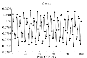
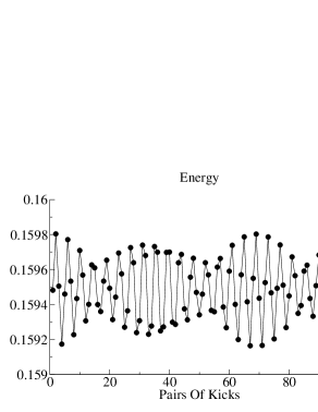
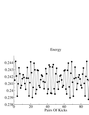
Figure 6.1: Right graphs show results obtained from equation (6.35) and left graphs show the same results obtained numerically. Top. $k=1,g=1$. Medium position. $k=1$,$g=2$. Bottom. $k=2$,$g=2$. Energy is measured in terms of the recoil energy given in equation (6.3).

where $\omega_{j}=\frac{\epsilon_{j}T}{2}$. This wave function reads $\frac{1}{\sqrt{2\pi}}$ for $\epsilon=0$ or $k=0$ as expected. In order to check the accuracy of equation (6.35) we calculate the state energy by the formula,

$$E(N)=\int_{0}^{2\pi}d\theta\psi^{*}(N)\left(-\frac{1}{2}\frac{\partial^{2}}{\partial\theta^{2}}+\frac{1}{2}g|\psi(N)|^{2}\right)\psi(N),$$ (6.36)

and compare it with computer simulations that use fast Fourier transform to shift the state wave function from position to momentum representation and vice versa. The graphs in figure 6.1 show in detail the energy oscillations for different values of $k$ and $g$ both from numerical simulations and from wave function (6.35). Outstandingly, both approaches agree quite well over a wide range of parameters.

6.2 Stability Analysis

So far we have considered the condensate as an isolated system. However, in a more realistic model particles in the ground state interact with particles in levels of higher energy and this causes bosons to escape from the condensate. Both the repulsion as well as the constant kicking determine the system stability. The second quantized analogous of the GP equation is given by [85],

$$\hat{H}=\int_{0}^{2\pi}d\theta\left(\hat{\psi^{\dagger}}\hat{h}\hat{\psi}+\frac{g}{2}\hat{\psi^{\dagger}}\hat{\psi^{\dagger}}\hat{\psi}\hat{\psi}\right),$$ (6.37)

where,

$$\hat{h}=-\frac{1}{2}\frac{\partial^{2}}{\partial\theta^{2}}+W(\theta,t),$$ (6.38)

$$W(\theta,t)=\left(-i\frac{\epsilon k}{2}\cos\theta+\frac{\epsilon k^{2}}{2}\sin^{2}\theta\right)\left(\sum_{n=0}^{\infty}{\delta(t-n(T))}\right).$$

In a perturbative approach the field operator can be written as,

$$\hat{\psi}(\theta,t)=\psi(\theta,t)\hat{a}_{0}+\delta\hat{\psi}(\theta,t),$$ (6.39)

where $\psi(\theta,t)$ is the ground state wave function of the condensate, given by equation (6.35). $\hat{a}_{0}$ and $\delta\hat{\psi}(\theta,t)$ are the bosonic operators for particles in and out the condensate respectively. Hamiltonian (6.37) must be inserted in the Heisenberg equations of motion and then these equations must be analytically integrated to get the Heisenberg dynamical operators. Ideally, the number of non-condensed particles (NNP) can be obtained by adding up the number of particles in excited modes. However, this can be rarely done directly due to the non-linearity of the original Hamiltonian. For this reason we use the method of reference [85], where practical equations in the linear response regime are proposed for the non-condensate cloud. From this work we now borrow the following identity,

$$\left(\begin{array}[]{c}\hat{\Lambda}(\theta,t)\\ \hat{\Lambda}^{\dagger}(\theta,t)\end{array}\right)=\sum_{j}\left\{\hat{b}_{j}\left(\begin{array}[]{c}U_{j}(\theta,t)\\ V_{j}(\theta,t)\end{array}\right)+\hat{b}^{\dagger}_{j}\left(\begin{array}[]{c}V^{*}_{j}(\theta,t)\\ U^{*}_{j}(\theta,t)\end{array}\right)\right\},$$ (6.40)

where,

$$\hat{\Lambda}=\frac{1}{\sqrt{\hat{N}}}\hat{a}^{\dagger}_{0}\delta\hat{\psi}.$$ (6.41)

Although $\hat{\Lambda}$ is not the non-condensate field operator itself, it is relevant to the number of particles off the condensate since,

$$\delta\hat{\psi}^{\dagger}\delta\hat{\psi}\approx\hat{\Lambda}^{\dagger}\hat{\Lambda},$$ (6.42)

in the low temperature limit [85]. The number of excitations for each mode in equation (6.40) is completely determined by the temperature through the well known Bose-Einstein distribution,

$$\langle\hat{b}_{j}^{\dagger}\hat{b}_{j}\rangle=\frac{1}{e^{\beta E_{j}}-1},$$ (6.43)

where $\beta=\frac{1}{k_{B}T}$. At zero temperature $\langle\hat{b}_{j}^{\dagger}\hat{b}_{j}\rangle=0$ and NNP is dictated only by the components of $U_{j}(\theta,t)$ and $V_{j}(\theta,t)$ in the space orthogonal to $\psi(\theta,t)$. The evolution of $U_{j}(\theta,t)$ and $V_{j}(\theta,t)$ is dictated by,

$$i\frac{\partial}{\partial t}\left(\begin{array}[]{c}U_{j}(\theta,t)\\ V_{j}(\theta,t)\end{array}\right)=$$ (6.46)

$$\left(\left(\begin{array}[]{cc}-\frac{1}{2}\frac{\partial^{2}}{\partial\theta^{2}}&0\\ 0&\frac{1}{2}\frac{\partial^{2}}{\partial\theta^{2}}\end{array}\right)+\left(\begin{array}[]{cc}W&0\\ 0&-W\end{array}\right)+\left(\begin{array}[]{cc}2g|\psi|^{2}&g\psi^{2}\\ -g{\psi^{*}}^{2}&-2g|\psi|^{2}\end{array}\right)\right)\left(\begin{array}[]{c}U_{j}(\theta,t)\\ V_{j}(\theta,t)\end{array}\right),$$ (6.55)

with $W=W(\theta,t)$ and $\psi=\psi(\theta,t)$. Additionally, NNP can be written as,

$$NNP=\sum_{j}\langle V_{j}|\hat{Q}\hat{Q}|V_{j}\rangle,$$ (6.56)

with,

$$\hat{Q}=\hat{1}-|\psi\rangle\langle\psi|,$$ (6.57)

in the limit of very low temperature. In order to carry out our numerical analysis, we first integrate the GP equation (6.1) using a fast Fourier transform algorithm and get the wave function $\psi(\theta,t)$. Then we insert this $\psi(\theta,t)$ into equation (6.46) and integrate for the initial conditions (6.81). Finally, we calculate NNP using equation (6.56).

6.3 Evolution of the number of non-condensed particles

Equation (6.56) is the same as

$$NNP=\sum_{j}\left\{\langle V_{j}|V_{j}\rangle-|\langle\psi|V_{j}\rangle|^{2}\right\}.$$ (6.58)

Moreover, as $\psi$ is normalized to 1, NNP is always positive and dependent on $\langle V_{j}|V_{j}\rangle$. Correspondingly, we focus on finding the norm of $V_{j}(\theta,t)$ since it provides us with quality information regarding the NNP. For $g=0$, $U_{j}(\theta,t)$ and $V_{j}(\theta,t)$ become decoupled in equation (6.46) and both functions undergo unitary evolution that leaves the norm unchanged. This implies that norm diffusion is exclusively due to the non-linear term of equation (6.46). In order to explore how the norm of $V_{j}(\theta,t)$ behaves in time, we highlight how the non-linear term acts on the state vector, namely,

$$\left(\begin{array}[]{c}U_{j}(\theta,t+\Delta)\\ V_{j}(\theta,t+\Delta)\end{array}\right)=e^{i\Delta\hat{G}(\theta,t)}\left(\begin{array}[]{c}U_{j}(\theta,t)\\ V_{j}(\theta,t)\end{array}\right),$$ (6.59)

where,

$$\hat{G}(\theta,t)=\left(\begin{array}[]{cc}2g|\psi(\theta,t)|^{2}&g\psi(\theta,t)^{2}\\ -g{\psi(\theta,t)^{*}}^{2}&-2g|\psi(\theta,t)|^{2}\end{array}\right).$$ (6.60)

As can be seen, operator $\hat{G}$ is not hermitian, which is by no means inconsistent, since further exploration shows that the eigenvalues of $\hat{G}$ are themselves real. This is an important issue to consider when exploring the development of NNP. In fact, according to [92], the norm of the $U_{j}$-$V_{j}$ vector (global norm) is given by,

$$\left(\langle U_{j}|,-\langle V_{j}|\right)\left(\begin{array}[]{c}|U_{j}\rangle\\ |V_{j}\rangle\end{array}\right)=\int_{0}^{2\pi}d\theta|U_{j}(\theta,t)|^{2}-\int_{0}^{2\pi}d\theta|V_{j}(\theta,t)|^{2}=Constant,$$ (6.61)

with $Constant=1$ for all $j$. As can be seen, the norm of $V_{j}(\theta,t)$ can grow indefinitely as long as the difference of the two norms remains constant. Notice that norm growing depends heavily on the definition of inner product in the Hilbert space. If we had $+$ instead of $-$ above the norm of $V_{j}(\theta,t)$ and $U_{j}(\theta,t)$ would be bounded by $Constant$. Making use of norm conservation properties we now write the state vector as,

$$\left(\begin{array}[]{c}U_{j}(\theta,t)\\ V_{j}(\theta,t)\end{array}\right)=\left(\begin{array}[]{c}\sinh\left(\alpha_{j}(t)\right)u_{j}(\theta,t)\\ \cosh\left(\alpha_{j}(t)\right)v_{j}(\theta,t)\end{array}\right),$$ (6.62)

$u_{j}(\theta,t)$ and $v_{j}(\theta,t)$ are complex functions normalized to unity while $\alpha_{j}(t)$ is a real function that characterizes the norm of $V_{j}(\theta,t)$ and $U_{j}(\theta,t)$. In order to gain insight into the evolution of the norm of $U_{j}(\theta,t)$ and $V_{j}(\theta,t)$, or equivalently, the evolution of $\alpha(t)$, we explicitly perform the operation indicated in equation (6.59) following a similar procedure as in reference [93]. In doing so we find that matrix $\hat{G}$ can be written as (let us omit the dependence with $\theta$ and $t$ for simplicity),

$$\hat{G}=\left(\begin{array}[]{cc}2g|\psi|^{2}&g|\psi|^{2}e^{i\phi}\\ -g|\psi|^{2}e^{-i\phi}&-2g|\psi|^{2}\end{array}\right),$$ (6.63)

with the following eigenvectors (not normalized),

$$\langle\theta|E_{+})=\left(\begin{array}[]{c}e^{2i\phi(\theta,t)}\\ \sqrt{3}-2\end{array}\right),\hskip 14.22636pt\lambda_{+}=\sqrt{3}g|\psi(\theta,t)|^{2},$$ (6.66)

$$\langle\theta|E_{-})=\left(\begin{array}[]{c}e^{2i\phi(\theta,t)}\\ -(\sqrt{3}+2)\end{array}\right),\hskip 14.22636pt\lambda_{-}=-\sqrt{3}g|\psi(\theta,t)|^{2}.$$ (6.69)

From equation (6.59) we can infer,

$$\left(\begin{array}[]{c}|U_{j}\rangle\\ |V_{j}\rangle\end{array}\right)_{t+\Delta}=\left(\mu_{j}e^{i\lambda_{+}\Delta}|E_{+})+\nu_{j}e^{i\lambda_{-}\Delta}|E_{-})\right)_{t}.$$ (6.70)

Scalars $\mu_{j}(\theta,t)$ and $\nu_{j}(\theta,t)$ can be written in terms of $U_{j}(\theta,t)$ and $V_{j}(\theta,t)$ making use of this equation with $\Delta=0$. In doing so we find,

$$\mu_{j}(\theta,t)=\frac{(\sqrt{3}-2)V_{j}(\theta,t)-e^{-2i\phi(\theta,t)}U_{j}(\theta,t)}{2(3-2\sqrt{3})},$$ (6.71)

$$\nu_{j}(\theta,t)=-\frac{(\sqrt{3}+2)V_{j}(\theta,t)+e^{-2i\phi(\theta,t)}U_{j}(\theta,t)}{2(3+2\sqrt{3})}.$$ (6.72)

At this point it is worth noticing that global-norm conservation is a direct consequence of,

$$(E_{-}|E_{+})=0.$$ (6.73)

Now, let us introduce the symbol $[...|...]$ to describe an inner product as in equation (6.61) but with $+$ instead of $-$, so that we can address the following “global-norm”,

$$\left(\langle U_{j}|U_{j}\rangle+\langle V_{j}|V_{j}\rangle\right)_{t+\Delta}=$$ (6.74)

$$\left([E_{+}||\mu_{j}|^{2}|E_{+}]+[E_{-}||\nu_{j}|^{2}|E_{-}]+[E_{+}|\mu_{j}^{*}\nu_{j}e^{-2i\lambda_{+}\Delta}|E_{-}]+[E_{-}|\nu_{j}^{*}\mu_{j}e^{2i\lambda_{+}\Delta}|E_{+}]\right)_{t},$$

where use has been made of equation (6.70). If we expand exponentials to first order in $\Delta$ we obtain,

$$\left(\langle U_{j}|U_{j}\rangle+\langle V_{j}|V_{j}\rangle\right)_{t+\Delta}=\left(\langle U_{j}|U_{j}\rangle+\langle V_{j}|V_{j}\rangle\right)_{t}+$$ (6.75)

$$2i\Delta\left([E_{-}|\lambda_{+}\nu_{j}^{*}\mu_{j}|E_{+}]-[E_{+}|\lambda_{+}\mu_{j}^{*}\nu_{j}|E_{-}]\right)_{t},$$

hence it follows,

$$\frac{\left(\langle U_{j}|U_{j}\rangle+\langle V_{j}|V_{j}\rangle\right)_{t+\Delta}-\left(\langle U_{j}|U_{j}\rangle+\langle V_{j}|V_{j}\rangle\right)_{t}}{\Delta}=$$ (6.76)

$$2i\left([E_{-}|\lambda_{+}\nu_{j}^{*}\mu_{j}|E_{+}]-[E_{+}|\lambda_{+}\mu_{j}^{*}\nu_{j}|E_{-}]\right)_{t},$$

which amounts to,

$$-8\sqrt{3}g\int_{0}^{2\pi}d\theta|\psi|^{2}Im(\nu_{j}^{*}\mu_{j}).$$ (6.77)

So, using (6.71) and (6.72) to write the integral above in terms of $U_{j}$ and $V_{j}$ we get,

$$\frac{d}{dt}\left(\langle U_{j}|U_{j}\rangle+\langle V_{j}|V_{j}\rangle\right)=-4g\int_{0}^{2\pi}d\theta|\psi|^{2}Im(e^{2i\phi}V_{j}U_{j}^{*}).$$ (6.78)

This expression can be further simplified by writing it in terms of $\alpha_{j}(t)$ as defined in equation (6.62),

$$\frac{d}{dt}\left(\sinh^{2}\alpha_{j}+\cosh^{2}\alpha_{j}\right)=-4g\sinh\alpha_{j}\cosh\alpha_{j}\int_{0}^{2\pi}d\theta Im(\psi^{2}u_{j}^{*}v_{j}).$$ (6.79)

Finally, using well known identities we arrive to

$$\frac{d\alpha_{j}}{dt}=-g\int_{0}^{2\pi}d\theta Im(\psi^{2}u_{j}^{*}v_{j}).$$ (6.80)

This equation determines the evolution of the state norm in our problem. Let us point out that this equation is valid for arbitrary $t$ since both the dynamical term as well as the static potential in equation (6.46) do not affect the state norm. Now equation (6.80) can be used to understand some aspects of NNP evolution. Indeed, for $t=0$ all the variables in the integral are known, namely,

$$\psi=\frac{1}{\sqrt{2\pi}},\hskip 14.22636ptu_{j}=\frac{e^{ij\theta}}{\sqrt{2\pi}},\hskip 14.22636ptv_{j}=\frac{e^{ij\theta}}{\sqrt{2\pi}},$$ (6.81)

from which it follows,

$$\left.\frac{d\alpha_{j}}{dt}\right|_{t=0}=0.$$ (6.82)

Consequently, as long as the kicking is not strong enough to drive the condensate and the modes out their initial states, the NNP will remain constant (not necessarily zero). This behaviour is positively corroborated by the graphs that we show in figure 6.2-left, where the NNP is plotted against the number of kicks. As can be seen from this graph, dissipation is quite moderate even after several tens of kicks.

Figure 6.2: Left. $\beta=1.96$, $\epsilon=0.04$. It is seen how NNP is hardly altered for weak kicking. Right. $k=1$, $g=1$. Momentum distribution for $\psi$ and $u_{1}$ after 160 kicks (80 pairs of kicks). After several kicks the momentum distributions still look very similar to the initial ones. The condensate and the modes develop opposite phases and the integral in equation (6.80) vanishes.

Figure 6.3 shows the behaviour of NNP for different values of the parameters $g$ and $k$. Initially, NNP does not respond to the kicking, which corresponds to the time that the system takes to evolve away from the initial conditions, in which case particle diffusion is given by equation (6.82). Once this initial unresponsiveness is over, NNP starts to develop in a characteristic manner. In the small interaction regime, NNP-growth becomes linear with a slope equal to 2. Empirically, this dissipation is tolerable and the condensate can be considered as stable [53, 84]. In contrast, for $g=5$ NNP-growth becomes exponential, which unequivocally characterizes the unstable phase. Figure 6.3-right shows the slopes of several curves of NNP as they are all fitted to exponential behaviour. Although exponential behaviour may not be the most suitable fitting for every curve, it allows us to put our results in a comparative perspective. Figure 6.3-right indicates that the system response is notably intense around some sections of the horizontal axis. This strong response arises when the kick frequency coincides or is close to one of the natural frequencies of the condensate, which are given by $\omega_{1}$ and $\omega_{2}$ in equation (6.35) [94]. This effect is analogous to the resonances of mechanical systems, which occur when the driving frequency coincides with one of the system’s natural frequencies. In this way, the strong resonance driving triggers particle dissipation and hence destroys the condensate. We point out that this is different from instability due to linear resonances, which take place when the contributions from different kicks interact coherently. In fact, these latter resonances are known to lead to chaos in the classical realm [89, 90, 88, 87].

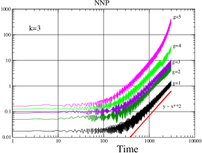
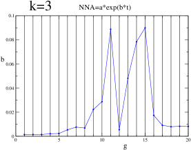
Figure 6.3: Left. $\beta=1.96$, $\epsilon=0.04.$ In the strong repulsion regime NNP grows exponentially and the condensate becomes unstable. Time is measured in numbers of pairs of kicks

. Right. Slope $b$ characterizes the intensity of particle leakage in the condensate. As can be seen, diffusion peaks around some values of $g$, evidencing the effect of resonances.

Here we have studied the wave function of a double-kicked BEC as well as the stability of the system. We have derived analytical expressions for the condensate wave function in the linear response regime. From the solution of the Gross-Pitaevskii equation, we identified resonance conditions for which particle dissipation is maximum. Our findings were verified by numerical simulations using a fast Fourier transform algorithm. We also investigated the second quantized Hamiltonian and established useful formulae regarding the dynamics of the NNP. Our study is relevant to experiments of cold atoms in optical lattices and our results are interesting from a purely theoretical viewpoint.

6.4 Advancements in the field

Since the presentation of our results in 2007, there has been further progress on the subject of condensate stability. Here we want to summarize the main results of these interesting works in order to provide a complete view of the actual state of the topic.

A complete characterization of the condensate stability has been reported in [84], including a map of the stability parameters showing the position of the resonances for weak and strong interactions. In such reference the authors study how the non-linear response due to the interaction among atoms affects the well understood linear response, for which linear resonances have been studied and characterized. In this latter case, it is known that resonances are located at integer multiples of the so called Talbot time, $T=4\pi$. It was found that the non-linear dynamics not only displaces the positions of the linear resonances but also affects the nature of the response. Specifically, it is shown that in the range $1\leq g\leq 20$ the resonance response is characterized by a sharp cut-off of the NNP and therefore the condensate revives after it has lost stability. The non-linear resonances manifest individually for small values of $g$ and $k$, but they progressively proliferate and overlap as the parameters are slowly tuned up. Likewise, the results of simulations using the GP equation are compared against the results of a second quantized model constructed from the insight provided by previous studies of the kicked-rotor dynamics [86]. It is shown that by including Beliaev and Landau terms coming from phonon-phonon interactions it is possible to reproduce the sharp fall in NNP close to a resonance as well as the shift in the position of the resonance in regimes where depletion of the ground state is $\leq 10\%$. Conversely, the same approach fails to reproduce the condensate dynamics when such terms are not taken into consideration. The second quantized model clarifies many issues regarding the depletion process and helps understand how resonances overlap and also how the cut-off process takes place. In the second quantized approach the condensate revival appears as a combination of Beliaev and Landau processes, in a way that is very similar to non-linear self-trapping of a BEC in a double-well potential. Certainly, the cut-off phenomenon can be understood by the following first principle analysis. When the condensate is being kicked slightly off-resonance, the interaction drives particles from the condensate towards the first excited mode. This triggers particle migration to the second mode, which at the same time induces a phase shift that brings the first mode closer into resonance. This is known as non-linear feedback and it is specially responsible for the strong condensate depletion seen before the cut-off. However, if the kicking is not sufficiently close to resonance, the synchronization process among excited modes does not occur and depletion is suppressed, which results in the abrupt cut-off reported in reference [84]. Further inspection suggests that the intensity of the cut-off is much sharper than in double-well condensates. Moreover, the resonances are classified in two basic categories. First, linear resonances, which derive from the Talbot resonances and are seen to be parametrically displaced by the non-linearity. These lead to strong, high amplitude response. Second, non-linear resonances, which disappear when $g=0$. Such resonances can arise individually, as Bogoliubov modes, or in combination of two or more modes. Non-linear response is weaker than linear response, but surprisingly, a Lyapunov analysis reveals that non-linear resonances are unstable, contrary to linear resonances. A possible explanation of this is that non-linear resonances are linked to exponential oscillations and therefore the Lyapunov stability criterion becomes questionable. Finally, the stability profile could be used in applications where very sharp excitation thresholds are needed to carry out high accuracy measurements, as for example measuring gravity or detecting small changes of frequency in rotating BEC’s.

Conclusions

In this work we have adjusted recently developed numerical methods to probe the ground state as well as the dynamics of bosonic systems. In addition, we have introduced a numerical method that displays some advantages over standard approaches, and we applied it to solve challenging problems.

In the first part of the document, we presented the concepts and ideas that we subsequently used along most of the work. As numerics is an important part of this research, we extensively discussed how our programs were constructed and how they work. We then discussed alternative uses of MPS in cases where analytical solutions for the Heisenberg operators are available. The efficiency and reliability of our method was tested, first in simple scenarios, and then in more complex situations. The most important application of the method in this work was to find the state of a system of bosons initially prepared in a separable state after a many particle collision has taken place in the centre of the chain. This calculation would have been much more difficult to do using TEBD or tDMRG as both of these methods are suitable only for short-time intervals. Likewise, we also derived analytically the conditions for an efficient collection of bosons on the chain terminals after the particle waves collide. This is an important point as in the absence of controlling mechanisms boson waves flatten and entanglement diffuses. Conversely, in our approach particles are collected so that the entanglement contained in the system as a result of the collision can be used. Our graphs show that the entanglement generated in this way is quite substantial and it is shown that such entanglement can be made to grow by just adding more particles to the process.

We next focus on applications of TEBD to the BH model, aiming at enhancing the amount of entanglement between the ends of the chain, either in the ground state or as a result of dynamics. We show that EEE in the ground state scales logarithmically with a positive coefficient when a hopping profile with perfect transmission properties is incorporated in the Hamiltonian. We conclude that such effect is due to a marked change in the tunnelling profile, which undergoes a transition from local to global scope. We use the real-time version of TEBD to simulate the dynamics of a chain with high repulsion in intermediate sites. The amount of entanglement generated out of dynamics alone is smaller than what can be obtained from the ground state. We then use a scheme that combines both ground state and dynamics to generate entanglement. Our results indicate that it is in fact possible to use dynamics to increase the amount of entanglement contained in the ground state by taking advantage a perturbative scheme that we have introduced.

In the last part we concentrate on kicked bosonic systems. We utilized a perturbative approach to obtain an analytical expression for the bosonic cloud in the linear response regime. Additionally, we derived useful formulae regarding the number of non-condensed particles. We find that the condensate is highly depleted by a kicking with a driving frequency that matches any of the natural frequencies of the system. Similarly, we have reviewed the latest advances in the field.

Among the several potential research extensions of the present work we would like to mention the possibility of studying chains with periodic boundary conditions, where vortices are expected to appear. Also, the numerical method presented here is liable of improvement. Indeed, it seems plausible that the method can be formulated without the need for an explicit solution of the Heisenberg equations of motion for the operators. The procedure can be applied to a wide variety of problems, not only in linear arrangements, but also in lattices, since in our method the geometry of the system does not interfere with the reduction process. Potential extensions of the method to spin and fermionic systems are quite direct. Additionally, it would be very interesting to implement the configuration proposed in chapter 5 in an actual experiment, since such configuration can be realized in optical lattices using state-of-the-art technology. One of the main conclusions of this work is the enhancement of entanglement in chains with PTH hopping. Similarly, as repulsion constants are turned up in the middle, we can think of intermediate places as forming a quantum wire. Therefore, it should be interesting to study a system made up of two particle-reservoirs connected by a quantum wire. As the infinity-repulsion BH model is known to derive in the $XX$ model, it is likely that a problem like this can be solved analytically. If this is the case, it should be possible to establish the actual relation between the hopping profile and entanglement.

The present has been an interdisciplinary investigation that covered areas such as numerical methods, many-body systems, quantum information and so on. Our findings help understand how entanglement relates to some physical processes that occur in bosonic systems. Such understanding can be used in different ways, as for example, to propitiate the circumstances that are convenient to produce entanglement in an experiment, or just as a way of appreciating the phenomenology of bosonic systems from a different perspective. Altogether, we hope our contribution to be sufficiently relevant so that it can inspire further investigation in any of the very exciting scientific fields with which this research overlaps.

Appendix A: Publications

• Jose Reslen and Sougato Bose, Long Range Free Bosonic Models in Block Decimation Notation: Applications and Entanglement, arXiv:0907.4315. Submitted.

• Jose Reslen and Sougato Bose, End-to-end entanglement in Bose-Hubbard chains. Physical Review A, 80: 012330, (2009).

• J. Reslen, C.E. Creffield and T.S. Monteiro, Dynamical instability in kicked Bose-Einstein condensates: Bogoliubov resonances. Physical Review A, 77: 043621, (2008).

Bibliography

- [1] M.H. Anderson, J.R. Ensher, M.R. Matthews, C.E. Wieman, and E.A. Cornell. Observation of Bose-Einstein condensation in a dilute atomic vapor. Scince, 269:198, 1995.
- [2] K.B. Davis, M.-O. Mewes, M.R. Andrews, N.J. van Druten, D.S. Durfee, D.M. Kurn, and W. Ketterle. Bose-Einstein condensation in a gas of sodium atoms. Physical Review Letters, 75:3969, 1995.
- [3] A.F. Ho, M.A. Cazalilla, and T. Giamarchi. Quantum simulation of the Hubbard model: the attractive route. Physical Review A, 79:033620, 2009.
- [4] M.P.A. Fisher, P.B. Weichman, G. Grinstein, and D.S. Fisher. Boson localization and the superfluid-insulator transition. Physical Review A, 40:546, 1989.
- [5] D. Jaksch, C. Bruder, J.I. Cirac, C.W. Gardiner, and P. Zoller. Cold bosonic atoms in optical lattices. Physical Review Letters, 81:3108, 1998.
- [6] M. Greiner, O. Mandel, T. Esslinger, T. W. Hansch, and I. Bloch. Quantum phase transition from a superfluid to a Mott insulator in a gas of ultracold atoms. Nature, 415:39, 2002.
- [7] T. Stoferle, H. Moritz, C. Schori, M. Kohl, and T. Esslinger. Transition from a strongly interacting 1d supefluid to a Mott insulator. Physical Review Letters, 92:130403, 2004.
- [8] U. Schnorrberger, J.D. Thompson, S. Trotzky, R. Pugatch, N. Davidson, S. Kuhr, and I. Bloch. Electromagnerically induced transparency and light storage in an atomic Mott insulator. Physical Review Letters, 103:033003, 2009.
- [9] C.A. Regal, M. Greiner, and D.S. Jin. Observation of resonance condensation of fermionic atom pairs. Physical Review Letters, 92:040403, 2004.
- [10] T. Bourdel, L. Khaykovich, J. Cubizolles, J. Zhang, F. Chevy, M. Teichmann, L. Tarruell, S.J.J.M.F. Kokkelmans, and C. Salomon. Experimental study of the BEC-BCS crossover region in Lithium 6. Physical Review Letters, 93:050401, 2004.
- [11] J.J. Chang, P. Engels, and M.A. Hoefer. Formation of dispersive shock waves by merging and splitting Bose-Einstein condensates. Physical Review Letters, 101:170404, 2008.
- [12] I.B. Spielman, W.D. Phillips, and J.V. Porto. Mott-insulator transition in a two-dimensional atomic Bose gas. Physical Review Letters, 98:080404, 2007.
- [13] Th. Best, S. Will, U. Schneider, L. Hackermuller, D. van Oosten, I. Bloch, and D.-S. Luhmann. Role of interactions in 87Rb-40K Bose-Fermi mixtures in a 3D optical lattice. Physical Review Letters, 102:030408, 2009.
- [14] C.D. Fertig, K.M. O’Hara, J.H. Huckans, S.L. Rolston, W.D. Phillips, and J.V. Porto. Strongly inhibited transport of a degenerate 1D bose gas in a lattice. Physical Review Letters, 94:120403, 2005.
- [15] P. Cheinet, S. Trotzky, M. Feld, U. Schnorrberger, M. Moreno-Cardoner, S. Folling, and I. Bloch. Counting atoms using interaction blockade in an optical superlattice. Physical Review Letters, 101:090404, 2008.
- [16] S. Folling, S. Trotzky, P. Cheinet, M. Feld, R. Saers, A. Widera, T. Muller, and I. Bloch. Direct observation of second-order atom tunnelling. Nature, 448:1029, 2007.
- [17] M. Radmark, M. Zukowski, and M. Bourennane. Experimental test of fidelity limits in six-photon interferometry and of rotational invariance properties of the photonic six-qubit entanglement singlet state. Physical Review Letters, 103:150501, 2009.
- [18] S. Olmschenk, D.N. Matsukevich, P. Maunz, D. Hayes, L.-M. Duan, and C. Monroe. Quantum teleportation between distant matter qubits. Science, 323:486, 2009.
- [19] S.R. White. Density matrix formulation for quantum renormalization groups. Physical Review Letters, 69:2863, 1992.
- [20] S.R. White. Density matrix algorithms for quantum renormalization groups. Physical Review B, 48:345, 1993.
- [21] G. Vidal. Efficient classical simulation of slightly entangled quantum computations. Physical Review Letters, 91:147902, 2003.
- [22] G. Vidal. Efficient simulation of one-dimensional quantum many-body systems. Physical Review Letters, 93:040502, 2004.
- [23] G. Vidal. Classical simulation of infinite-size quantum lattice systems in one spatial dimension. Physical Review Letters, 98:070201, 2007.
- [24] G. Vidal. Entanglement renormalization. Physical Review Letters, 99:220405, 2007.
- [25] G. Vidal. Class of quantum many-body states that can be efficiently simulated. Physical Review Letters, 101:110501, 2008.
- [26] F. Verstraete, V. Murg, and J.I. Cirac. Matrix product states, projected entangled pair states, and variational renormalization group methods for quantum spin systems. Advances in Physics, 57:143, 2008.
- [27] M.J. Hartmann, J. Prior, S.R. Clark, and M.B. Plenio. Density matrix renormalization group in the Heisenberg picture. Physical Review Letters, 102:057202, 2009.
- [28] S.R. Clark, J. Prior, M.J. Hartmann, D. Jaksch, and M.B. Plenio. Exact matrix product solutions in the heisenberg picture of an open quantum spin chain. quant-ph/0907.5582.
- [29] S.R. White and A.E. Feiguin. Real time evolution using the density matrix renormalization group. Physical Review Letters, 93:076401, 2004.
- [30] S.R. White, D.J. Scalapino, R.L. Sugar, E.Y. Loh, J.E. Gubernatis, and R.T. Scalettar. Numerical study of the two-dimensional Hubbard model. Physical Review B, 40:506, 1989.
- [31] T.D. Kuhner and H. Monien. Phases of the one-dimensional Bose-Hubbard model. Physical Review B, 58:14741(R), 1998.
- [32] T.D. Kuhner, S.R. White, and H. Monien. One-dimensional Bose-Hubbard model with nearest-neighbor interaction. Physical Review B, 61:12474, 2000.
- [33] A.J. Daley, S.R. Clark, D. Jaksch, and P. Zoller. Numerical analysis of coherent many-body currents in a single atom transistor. Physical Review A, 72:043618, 2005.
- [34] M. Hartmann and M.B. Plenio. Migration of bosonic particles across a Mott insulator to a superfluid phase interface. Physical Review Letters, 100:070602, 2008.
- [35] R.V. Mishmash and L.D. Carr. Quantum entanglement dark solitons formed by ultracold atoms in optical lattices. Physical Review Letters, 103:140403, 2009.
- [36] R.V. Mishmash, I. Danshita, C.W. Clark, and L.D. Carr. cond-mat/0906.4949.
- [37] D. Muth, A. Mering, and M. Fleishhauer. Ultracold bosons in disordered superlattices: Mott insulators induced by tunneling. Physical Review A, 77:043618, 2008.
- [38] L. Mathey, I. Danshita, and C.W. Clark. Creating a supersolid in one-dimensional Bose mixtures. Physical Review A, 79:011602(R), 2009.
- [39] I. Danshita and C.W. Clark. Heavily damped motion of one-dimensional Bose gases in an optical lattice. Physical Review Letters, 102:030407, 2009.
- [40] S. Montangero, R. Fazio, P. Zoller, and G. Pupillo. Dipole oscillations of confined lattice bosons in one dimension. Physical Review A, 79:041602(R), 2009.
- [41] Nielsen M. A. and Chuang I. L. Quantum Computation and Quantum Information. Cambridge University Press, Cambridge, 2000.
- [42] L. Campos Venuti, C. Degli Esposti Boschi, and M. Roncaglia. Long-distance entanglement in spin systems. Physical Review Letters, 96:247206, 2006.
- [43] S. Bose. Quantum communication through an unmodulated spin chain. Physical Review Letters, 91:207901, 2003.
- [44] J.K. Stockton, J.M. Geremia, A.C. Doherty, and H. Mabuchi. Characterizing the entanglement of symmetric many-particle spin-1/2 systems. Physical Review A, 67:022112, 2003.
- [45] J. Reslen, L. Quiroga, and N.F. Johnson. Direct equivalence between quantum phase transition phenomena in radiation-matter and magnetic systems: Scaling of entanglement. Europhysics Letters, 69:8, 2005.
- [46] D.I. Tsomokos, M.J. Hartman, S.F. Huelga, and M.B. Plenio. Entanglement dynamics in chains of qubits with noise disorder. New Journal of Physics, 9:79, 2007.
- [47] L. Amico, R. Fazio, A. Osterloh, and V. Vedral. Entanglement in many body systems. Reviews of Modern Physics, 80:517, 2008.
- [48] M. Moeckel and S. Kehrein. Interaction quench in the Hubbard model. Physical Review Letters, 100:175702, 2008.
- [49] L. Tian, F. Fujiwara, T. Byrnes, and Y. Yamamoto. Recovery of hidden interference in Mott insulators. quant-ph/0705.2023.
- [50] J. Eisert, M.B. Plenio, S. Bose, and J. Hartley. Towards quantum entanglement in nanoelectromechanical devices. Physical Review Letters, 93:190402, 2004.
- [51] O. Romero-Isart, K. Eckert, C. Rodo, and A. Sanpera. Transport and entanglement generation in the Bose-Hubbard model. Journal of Physics A: Mathematical and Theoretical, 40:8019, 2007.
- [52] M.B. Plenio, J. Hartley, and J. Eisert. Dynamics and manipulation of entanglement in coupled harmonic systems with many degrees of freedom. New Journal of Physics, 6:36, 2004.
- [53] C. Zhang, J. Liu, M.G. Raizen, and Q. Niu. Transition to instability in a kicked Bose-Einstein condensate. Physical Review Letters, 92:054101, 2004.
- [54] J. Liu, C. Zhang, M.G. Raizen, and Q. Niu. Transition to instability in a periodically kicked Bose-Einstein condensate on a ring. Physical Review A, 73:013601, 2006.
- [55] F.L. Moore, J.C. Robinson, C.F. Bharucha, B. Sundaram, and M.G. Raizen. Atoms optical realization of the quantum -kicked rotor. Physical Review Letter, 75:4598, 1995.
- [56] J. Dunningham and V. Vedral. Nonlocality of a single particle. Physical Review Letters, 99:180404, 2007.
- [57] J. Dunningham, A. Rau, and K. Burnett. From pedigree cats to fluffy-bunnies. Science, 307:872, 2005.
- [58] M.B. Plenio and S. Virmani. An introduction to entanglement meausures. Quantum information and computation, 7(1), 2007.
- [59] M.O. Terra-Cunha, J. Dunningham, and V. Vedral. Entanglement in single-particle systems. Proceedings of the royal society A, 463:2277, 2007.
- [60] A. Peres. Separability criterion for density matrices. Physical Review Letters, 77:1413, 1996.
- [61] M. Horodecki, P. Horodecki, and R. Horodecki. Separability of mixed states: necessary and sufficient conditions. Physics Letters A, 223:1, 1996.
- [62] G. Vidal and R.F. Werner. Computable measure of entanglement. Physical Review A, 65:032314, 2002.
- [63] A.J. Daley, C. Kollath, U. Schollwock, and G. Vidal. Time-dependent density-matrix renormalization-group using adaptive effective Hilbert spaces. Journal of Statistical Mechanics: Theory and Experiment, P04005, 2004.
- [64] C. Di-Franco, M. Paternostro, and M.S. Kim. Perfect state transfer on a spin chain without state initialization. Physical Review Letters, 101:230502, 2008.
- [65] M.-H. Yung and S. Bose. Perfect state transfer, effective gates, and entanglement generation in engineered bosonic and fermionic networks. Physical Review A, 71:032310, 2005.
- [66] M. Christandl, N. Datta, A. Ekert, and A.J. Landahl. Perfect state transfer in quantum spin networks. Physical Review Letters, 92:187902, 2004.
- [67] L.-A. Wu, A. Miranowicz, X.B. Wang, Y.-X. Liu, and F. Nori. Perfect function transfer and interference effects in interacting boson lattices. Physical Review A, 80:012332, 2009.
- [68] S.R. Clark, C. Moura-Alves, and D. Jaksch. Efficient generation of graph states for quantum computation. New Journal of Physics, 7:124, 2005.
- [69] D. Jaksch, H.-J. Briegel, J.I. Cirac, C.W. Gardiner, and P. Zoller. Entanglement of atoms via cold controlled collisions. Physical Review Letters, 82:1975, 1999.
- [70] F. Schmuser and D. Janzing. Entanglement generation via scattering of two particles with hard-core repulsion. Physical Review A, 73:052313, 2006.
- [71] C.K. Law. Entanglement production in colliding wave packets. Physical Review A, 70:062311, 2004.
- [72] N.L. Harshman and P. Singh. Entanglement mechanisms in one-dimensional potential scattering. Journal of Physics A: Mathematical and Theoretical, 41:155304, 2008.
- [73] Sakurai J. J. Modern Quantum Mechanics. Addison-Wesley publishing company, 1985.
- [74] A.M. Rey, G. Pupillo, C.W. Clark, and C.J. Williams. Ultracold atoms confined in an optical lattice plus parabolic potential: A closed-form approach. Physical Review A, 72:033616, 2005.
- [75] R. Roth and K. Burnett. Dynamic structure factor of ultracold bose and fermi gases in optical lattices. Journal of Physics B: Atomic, Molecular and Optical Physics, 37:3893, 2004.
- [76] A. Perales and G. Vidal. Entanglement growth and simulation efficiency in one-dimensional quantum lattice systems. Physical Review A, 78:042337, 2008.
- [77] T.J. Osborne. Efficient approximation of the dynamics of one-dimensional quantum spin systems. Physical Review Letters, 97:157202, 2006.
- [78] A.M. Lauchli and C. Kollath. Spreading of correlations and entanglement after a quench in the one-dimensional Bose-Hubbard model. Journal of statistical mechanics: theory and experiment, P05018, 2008.
- [79] M. Cramer, C.M. Dawson, J. Eisert, and T. Osborne. Exact relaxation in a class of nonequilibrium quantum lattice systems. Physical Review Letters, 100:030602, 2008.
- [80] A. Flesch, M. Cramer, I.P. McCulloch, U. Schollwock, and J. Eisert. Probing local relaxation of cold atoms in optical superlattices. Physical Review A, 78:033608, 2008.
- [81] C. Kollath, A.M. Lauchli, and E. Altman. Quench dynamics and nonequilibrium phase diagram of the Bose-Hubbard model. Physical Review Letters, 98:180601, 2007.
- [82] J. Goold, L. Heaney, Th. Busch, and V. Vedral. Detection and engineering of spatial mode entanglement with ultracold bosons. Physical Review A, 80:022338, 2009.
- [83] C. Simon. Natural entanglement in Bose-Einstein condensates. Physical Review A, 66:052323, 2002.
- [84] T.S. Monteiro, A. Rancon, and J. Ruostekoski. Nonlinear resonances in -kicked Bose-Einstein condensates. Physical Review Letters, 102:014102, 2009.
- [85] Y. Castin and R. Dum. Low-temperature Bose-Einstein condensates in time-dependent traps: Beyond the U(1) symmetry-breaking approach. Physical Review A, 57:3008, 1998.
- [86] C.E. Creffield, S. Fishman, and T.S. Monteiro. Theory of 2-kicked quantum rotors. Physical Review E, 73:066202, 2006.
- [87] C.E. Creffield, G. Hur, and T.S. Monteiro. Localization-delocalization transition in a system of quantum kicked rotors. Physical Review Letters, 96:024103, 2006.
- [88] M.M.A. Stocklin and T.S. Monteiro. Classical momentum diffusion in double--kicked particles. Physical Review E, 74:026210, 2006.
- [89] S. Fishman, D.R. Grempel, and R.E. Prange. Temporal crossover from classical to quantal behavior near dynamical critical points. Physical Review A, 36:289, 1987.
- [90] D.R. Grempel and R.E. Prange. Quantum dynamics of a nonintegrable system. Physical Review A, 29:1639, 1984.
- [91] D.L. Shepelyansky. Delocalization of quantum chaos by weak nonlinearity. Physical Review Letters, 70:1787, 1993.
- [92] Y. Castin. edited by R. Kaiser et al. Coherent Atomic Matter Waves. EDP Sciences and Springer-Verlag, New York, 2001. pages 62-73.
- [93] C. Zhang. Numerical integration of time-dependent bogoliubov equation. www.ph.utexas.edu/ cwzhang/article/BogEq.pdf.
- [94] I. Dana and D.L. Dorofeev. General quantum resonances of the kicked particle. Physical Review E, 73:026206, 2006.
- [95] J. Reslen and S. Bose. Long range free bosonic models in block decimation notation: Applications and entanglement. quant-ph/0907.4315.
- [96] J. Reslen and S. Bose. End-to-end entanglement in Bose-Hubbard chains. Physical Review A, 80:012330, 2009.
- [97] J. Reslen, C.E. Creffield, and T.S. Monteiro. Dynamical instability in kicked Bose-Einstein condensates. Physical Review A, 77:043621, 2008.
- [98] L. Amico, R. Fazio, A. Osterloh, and V. Vedral. Entanglement in many-body systems. Reviews of Modern Physics, 80:517, 2008.
- [99] I. D’Amico, B.W. Lovett, and T.P. Spiller. Freezing distributed entanglement in spin chains. Physical Review A, 76:030302, 2007.
- [100] S.-J. Gu, S.-S. Deng, Y.-Q. Li, and H.-Q. Lin. Entanglement and quantum phase transition in the extended Hubbard model. Physical Review Letters, 93:086402, 2004.
- [101] L. Heaney, J. Anders, D. Kaszlikowski, and V. Vedral. Spatial entanglement from off-diagonal long-range order in a Bose-Einstein condensate. Physical Review A, 76:053605, 2007.
- [102] I. Danshita and P. Naidon. Bose-Hubbard ground state: extended Bogoliubov and variational methods compared with time-evolving block decimation. Physical Review A, 79:043601, 2009.
- [103] C.E. Creffield and T.S. Monteiro. Tuning the Mott transition in a Bose-Einstein condensate by multiple photon absortion. Physical Review Letters, 96:210403, 2006.
- [104] R.N. Palmer, A. Klein, and D. Jaksch. Optical lattice quantum Hall effect. Physical Review A, 78:013609, 2008.